Quantum Estimation Theory of Error and Disturbance in Quantum Measurement

Abstract

We formulate the error and disturbance in quantum measurement by invoking quantum estimation theory. The disturbance formulated here characterizes the non-unitary state change caused by the measurement. We prove that the product of the error and disturbance is bounded from below by the commutator of the observables. We also find the attainable bound of the product.

I Introduction

Heisenberg discussed a thought experiment about the position measurement of a particle by the $\gamma$-ray microscope and found the trade-off relation between the error $\varepsilon(\hat{x})$ in the position measurement and the disturbance $\eta(\hat{p})$ to the momentum caused by the measurement process $\eta(\hat{p})$ bib:indeterminacy :

$$\varepsilon(\hat{x})\eta(\hat{p})\gtrsim\hbar.$$ (1)

This inequality epitomizes the complementarity of quantum measurements: we cannot perform the measurement of an observable without causing disturbance to its canonically conjugate observable. At the inception of quantum mechanics, the Kennard-Robertson inequality bib:kennard ; bib:robertson

$$\Delta X\Delta Y\geq\frac{1}{2}|{\langle[\hat{X},\hat{X}]\rangle}|$$ (2)

was erroneously interpreted as the mathematical formulation of the trade-off relation of error and disturbance in quantum measurement, where ${\langle\hat{X}\rangle}:={\operatorname{Tr}[{\hat{\rho}}\hat{X}]}$ is the expectation value of $\hat{X}$ over the quantum state ${\hat{\rho}}$, the square bracket denotes the commutator, and $(\Delta X)^{2}:={\langle\hat{X}^{2}\rangle}-{\langle\hat{X}\rangle}^{2}$. However, $\Delta X$ does not depend on the measurement process. Thus, the Kennard-Robertson inequality reflects the inherent nature of a quantum system alone, and does not concern any trade-off relation of the error and disturbance in the measurement process.

By performing the measurement we obtain some pieces of the information about the quantum state. However, the measurement process causes a non-unitary state change and decreases the information on the post-measurement state. Since the information is conserved under the unitary process, it can characterize the non-unitary effects of the measurement process. Therefore, it is expected that there exist the trade-off relations between the information obtained by the measurement and the information on the post-measurement state.

Ozawa bib:ozawa discussed the measurement processes and defined the error and disturbance, and derive a trade-off relation. According to his trade-off relation, it is possible to construct the measurement scheme such that the product of the error and disturbance vanishes. However, this does not mean that we can obtain information about the observable without dicreasing the information about the canonically conjugate observable on the post-measurement state, since his definitions of the error and disturbance per se do not always give quantitative information concerning observables.

In this paper, we formulate the complementarity of quantum measurements in terms of the information. Among several types of information contents in quantum theory, we use the Fisher information which gives precision of the estimated value calculated from the measurement outcomes. Because the measurement is performed to know the expectation value of an observable $\hat{X}_{1}$, it is natural that the error is measured by the precision of the estimated value of ${\langle\hat{X}_{1}\rangle}$. The non-unitary state change caused by the measurement process hinders us from estimating the expectation value of the conjugate observable. Thus the disturbance is characterized by the Fisher information corresponding to the estimation from the outcome of the sequential measurement,

This paper is organized as follows. In Sec. II, we define the measurement error and disturbance by invoking quantum estimation theory. In Sec. III, we derive trade-off relations between the measurement error and disturbance. In Sec. IV, we summarize the main results of this paper and discuss some outstanding issues.

II Error and Disturbance in Quantum Measurement

II.1 Measurement Error

Suppose we have $n$ independent and identically distributed (i.i.d.) unknown quantum states ${\hat{\rho}}$ on $d$-dimensional Hilbert spaces. To know the expectation value ${\langle\hat{X}\rangle}:={\operatorname{Tr}[{\hat{\rho}}\hat{X}]}$ of an observable $\hat{X}$, suppose that we perform the same measurement described by meausrement operators ${\bm{M}}=\{{\hat{M}}_{i,a}\}$ bib:kraus , where the first index $i$ denotes the measurement outcome. The probability distribution of the measurement outcomes and the post-measurement state ${\hat{\rho}}^{\prime}$ are given by

$$p_{i}={\operatorname{Tr}\left[{\hat{\rho}}\sum_{a}{\hat{M}}_{i,a}^{\dagger}{\hat{M}}_{i,a}\right]}={\operatorname{Tr}[{\hat{\rho}}\hat{E}_{i}]},$$ (3)

$${\hat{\rho}}^{\prime}=\sum_{i,a}{\hat{M}}_{i,a}{\hat{\rho}}{\hat{M}}_{i,a}^{\dagger},$$ (4)

where $\bm{E}=\{\hat{E}_{i}\}$ is the positive operator-valued measure (POVM) corresponding to $\bm{M}$. If the measurement is the projection measurement, then the estimated value of ${\langle\hat{X}\rangle}$ is calculated by

$$X^{\text{est}}=\sum_{i}\alpha_{i}\frac{n_{i}}{n},$$ (5)

where $\alpha_{i}$ are the eigenvalues of $\hat{X}$, and $n_{i}$ is the number of times that the outcome $i$ is obtained ($n=\sum_{i}n_{i}$). In general, the measurement error affects the outcomes, and thus the estimation of ${\langle\hat{X}\rangle}$ is nontrivial. A reasonable requirement to the estimators is the so-called consistency that for all quantum states ${\hat{\rho}}$ and an arbitrary $\delta>0$ the estimated value asymptotically converges to ${\langle\hat{X}\rangle}$:

$$\lim_{n\rightarrow\infty}\text{Prob}(|X^{\text{est}}-{\langle\hat{X}\rangle}|<\delta)=1.$$ (6)

An example of the consistent estimator is the maximum likelihood estimator. Since the estimated value is calculated from the measurement outcomes, the estimator of ${\langle\hat{X}\rangle}$ is a function of $\{n_{i}\}$: $X^{\text{est}}=X^{\text{est}}(\{n_{i}\})$. The expectation value and variance of the estimator $X^{\text{est}}$ are calculated to be

$$\operatorname{\mathbb{E}}[X^{\text{est}}]:=\sum_{\{n_{i}\}}p(\{n_{i}\})X^{\text{est}}(\{n_{i}\}),$$ (7)

$$\operatorname{Var}[X^{\text{est}}]:=\operatorname{\mathbb{E}}[(X^{\text{est}})^{2}]-\operatorname{\mathbb{E}}[X^{\text{est}}]^{2},$$ (8)

where the summation in (7) is taken over all sets $\{n_{i}\}$ that satisfy $n_{i}\geq 0$ and $\sum_{i}n_{i}=n$, and $p(\{n_{i}\})$ is the probability that each outcome $i$ is obtained $n_{i}$ times:

$$p(\{n_{i}\})=n!\prod_{i}\frac{p_{i}^{n_{i}}}{n_{i}!}$$ (9)

From (6), the average of the estimator satisfies

$$\lim_{n\rightarrow\infty}\operatorname{\mathbb{E}}[X^{\text{est}}]={\langle\hat{X}\rangle}.$$ (10)

The variance $\operatorname{Var}[X^{\text{est}}]$ is caused by three different kinds of errors: the quantum fluctuations, measurement errors and estimation errors (see Fig. 1). The estimation error arises unless we use optimal estimators that minimize $\operatorname{Var}[X^{\text{est}}]$ such asthe maximum likelihood estimator.

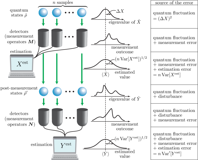
Figure 1: (Color online) Measurement process described by measurement operators $\bm{M}$ to know ${\langle\hat{X}\rangle}$. Due to the error in the measurement, the distribution of the measurement outcomes per se does not always provide the quantitative measurement error. To retrieve the information contained in the measurement outcomes, it is necessary to estimate ${\langle\hat{X}\rangle}$ from the measurement outcomes. The three types of errors described in the figure contribute to the variance of the estimated value $n\operatorname{Var}[X^{\text{est}}]$. By subtructing the quantum fluctuation and estimation error from $n\operatorname{Var}[X^{\text{est}}]$, the error inherent in the measurement process is obtained. Since the probability distribution on eigenvalues of $\hat{Y}$ on the post-measurement state ${\hat{\rho}}^{\prime}$ does not provide quantitative disturbance caused by the measurement $\bm{M}$, it is necessary to consider the sequential measurement and estimation process. The disturbance is quantified by subtracting the unwanted errors contained in the variance $n\operatorname{Var}^{\prime}[Y^{\text{est}}]$.

The variance $\operatorname{Var}[X^{\text{est}}]$ is bounded from below by the Cramér-Rao inequality bib:cramer :

$$\lim_{n\rightarrow\infty}n\operatorname{Var}[X^{\text{est}}]\geq\bm{x}^{\mathrm{T}}J({\bm{M}})^{-1}\bm{x},$$ (11)

where ${\mathrm{T}}$ denotes the transpose of the vector, $J({\bm{M}})$ is the Fisher information matrix

$$[J({\bm{M}})]_{\mu\nu}:=\sum_{i}p_{i}[\partial_{\mu}\log p_{i}][\partial_{\nu}\log p_{i}],$$ (12)

and the column vector $\bm{x}$ is given by

$$x_{\mu}=\partial_{\mu}{\langle\hat{X}\rangle},$$ (13)

with $\partial_{\mu}=\partial/\partial\theta_{\mu}$, and ${\bm{\theta}}=(\theta_{1},\dots,\theta_{d^{2}-1})$ are real parameters that characterize ${\hat{\rho}}$ such that any quantum state can be uniquely determined by specifing ${\bm{\theta}}$. The Fisher information matrix may have $0$ eigenvalues. The right-hand side (RHS) of (11) is calculated to be

$$\bm{x}^{\mathrm{T}}J({\bm{M}})^{-1}\bm{x}=\begin{cases}\bm{x}^{\mathrm{T}}J({\bm{M}})^{+}\bm{x},&\quad\bm{x}\in\operatorname{supp}[J({\bm{M}})],\\ +\infty,&\quad\text{otherwise},\end{cases}$$ (14)

where $J({\bm{M}})^{+}$ is the Moore-Penrose pseudoinverse of $J({\bm{M}})$. The case that the RHS of (11) is infinite means there exists no consistent estimator of ${\langle\hat{X}\rangle}$. It occurs, for example, by performing the projection measurement of an observable which does not commute with $\hat{X}$. If the RHS of the Cramér-Rao inequality (11) is finite, there always exist estimators that satisfy the equality of (11) such as the maximum likelihood estimator. Since such estimators minimize the variance, they are optimal to estimate ${\langle\hat{X}\rangle}$ from the measurement outcomes, and $\lim_{n\to\infty}n\operatorname{Var}[X^{\text{est}}]$ of the optimal estimators, equivalent to the RHS of (11), does not caused in the estimation process. Therefore, the RHS of (11) shows the quantum fluctuation and measurement error.

The RHS of (11) is independent of the specification of ${\hat{\rho}}$ by ${\bm{\theta}}$. Thus, we use the following parameterization.

$${\hat{\rho}}=d^{-1}\hat{I}+{\bm{\theta}}^{\mathrm{T}}{\hat{\bm{\lambda}}}=d^{-1}\hat{I}+\sum_{\mu}\theta_{\mu}\hat{\lambda}_{\mu},$$ (15)

where $\hat{I}$ is the identity operator, and ${\hat{\bm{\lambda}}}=\{\hat{\lambda}_{1},\dots,\hat{\lambda}_{d^{2}-1}\}$ is the generators of the Lie algebra $\mathfrak{su}(d)$. The generator ${\hat{\bm{\lambda}}}$ satisfy

$$\hat{\lambda}_{\mu}^{\dagger}=\hat{\lambda}_{\mu},\quad{\operatorname{Tr}[\hat{\lambda}_{\mu}]}=0,\quad{\operatorname{Tr}[\hat{\lambda}_{\mu}\hat{\lambda}_{\nu}]}=\delta_{\mu\nu}.$$ (16)

In terms of this generator, the observable $\hat{X}$, and the POVM $\bm{E}$ can be written as

$$\hat{X}=x_{0}\hat{I}+\bm{x}^{\mathrm{T}}{\hat{\bm{\lambda}}},$$ (17)

$${\hat{E}}_{i}=r_{i}\hat{I}+\bm{v}_{i}^{\mathrm{T}}{\hat{\bm{\lambda}}}.$$ (18)

The expectation value ${\langle\hat{X}\rangle}$ and the probability distribution can be calculated as

$${\langle\hat{X}\rangle}=x_{0}+\bm{x}^{\mathrm{T}}{\bm{\theta}},$$ (19)

$$p_{i}=r_{i}+\bm{v}_{i}^{\mathrm{T}}{\bm{\theta}}.$$ (20)

Then, the RHS of (11) can be calculated to be

$$\bm{x}^{\mathrm{T}}J({\bm{M}})^{-1}\bm{x}=\bm{x}^{\mathrm{T}}\left[\sum_{i}p_{i}^{-1}\bm{v}_{i}\bm{v}_{i}^{\mathrm{T}}\right]^{-1}\bm{x}.$$ (21)

The Fisher information matrix $J({\bm{M}})$ varies with varying ${\bm{M}}$, but it is bounded from above by the quantum Cramér-Rao inequality bib:caves:quantum-cramer-rao :

$$J({\bm{M}})\leq J_{Q},$$ (22)

where $J_{Q}$ is the quantum Fisher information, that depend only on quantum state ${\hat{\rho}}$. The quantum Fisher information is a monotone metric on the quantum state space with the coordinate system ${\bm{\theta}}$. Here, by monotone means that for any quantum operation $\mathcal{O}$ the following inequality is satisfied:

$$J_{Q}\geq J_{Q}^{\prime},$$ (23)

where $J_{Q}^{\prime}$ is the quantum Fisher information on $\mathcal{O}({\hat{\rho}})$. Although the quantum Fisher information is not uniquely determined, from the monotonicity condition there exist the minimum and the maximum bib:petz . The minimum is the symmetric logarithmic derivative (SLD) Fisher information $J_{S}$ bib:helstrom:quantum-fisher . The SLD Fisher information is a real symmetric matrix, whose $\mu\nu$-element is defined as

$$[J_{S}]_{\mu\nu}:=\frac{1}{2}{\operatorname{Tr}[{\hat{\rho}}\{\hat{L}_{\mu},\hat{L}_{\nu}\}]},$$ (24)

where the curly brackets $\{\ ,\ \}$ denote the anti-commutator, and $\hat{L}_{\mu}$ is a Hermitian operator called SLD operator defined as the solution to the following operator equation:

$$\partial_{\mu}{\hat{\rho}}=\frac{1}{2}\{{\hat{\rho}},\hat{L}_{\mu}\}.$$ (25)

The maximum quantum Fisher information is the right logarithmic derivative (RLD) Fisher information $J_{R}$. The RLD Fisher information is a Hermitian matrix, whose $\mu\nu$-element is defined as

$$[J_{R}]_{\mu\nu}:={\operatorname{Tr}[{\hat{\rho}}\hat{L}^{\prime}_{\nu}\hat{L}^{\prime}_{\mu}]},$$ (26)

where $\hat{L}^{\prime}_{\mu}$ is an operator called RLD operator defined as the solution to the following operator equation:

$$\partial_{\mu}{\hat{\rho}}={\hat{\rho}}\hat{L}^{\prime}_{\mu}.$$ (27)

The inverse of the SLD and RLD Fisher information matrices are calculated to be

$$[J_{S}^{-1}]_{\mu\nu}=\mathcal{C}_{s}(\hat{\lambda}_{\mu},\hat{\lambda}_{\nu}):=\frac{1}{2}{\langle\{\hat{\lambda}_{\mu},\hat{\lambda}_{\nu}\}\rangle}-{\langle\hat{\lambda}_{\mu}\rangle}{\langle\hat{\lambda}_{\nu}\rangle},$$ (28)

$$[J_{R}^{-1}]_{\mu\nu}=\mathcal{C}(\hat{\lambda}_{\mu},\hat{\lambda}_{\nu}):={\langle\hat{\lambda}_{\mu}\hat{\lambda}_{\nu}\rangle}-{\langle\hat{\lambda}_{\mu}\rangle}{\langle\hat{\lambda}_{\nu}\rangle},$$ (29)

where $\mathcal{C}_{s}$ and $\mathcal{C}$ are the symmetrized and non-symmetrized correlation functions. For the observables $\hat{X}=x_{0}\hat{I}+\bm{x}^{\mathrm{T}}{\hat{\bm{\lambda}}}$ and $\hat{Y}=y_{0}\hat{I}+\bm{y}^{\mathrm{T}}{\hat{\bm{\lambda}}}$,

$$\bm{x}^{\mathrm{T}}J_{S}^{-1}\bm{x}=\bm{x}^{\mathrm{T}}J_{R}^{-1}\bm{x}=(\Delta X)^{2},$$ (30)

$$\bm{x}^{\mathrm{T}}J_{S}^{-1}\bm{y}=\mathcal{C}_{s}(\hat{X},\hat{Y}),$$ (31)

$$\bm{x}^{\mathrm{T}}J_{R}^{-1}\bm{y}=\mathcal{C}(\hat{X},\hat{Y}).$$ (32)

From (22) and (30), the RHS of (11) is bounded from below as

$$\bm{x}^{\mathrm{T}}J({\bm{M}})^{-1}\bm{x}\geq(\Delta X)^{2}.$$ (33)

The equality is achieved if and only if $\bm{M}$ is the projection measurement of $\hat{X}$, that is the POVM $\bm{E}$ corresponding to $\bm{M}$ satisfies

$$\hat{E}_{i}\hat{E}_{i^{\prime}}=\delta_{ii^{\prime}}\hat{E}_{i},\hat{X}=\sum_{i}\alpha_{i}\hat{E}_{i}.$$ (34)

Since the left-hand side (LHS) shows the quantum fluctuation and measurement error, and the RHS is the quantum fluctuation, the difference of both sides gives the measurement error. We define the measurement error as

$$\varepsilon(\hat{X};{\bm{M}}):=\bm{x}^{\mathrm{T}}J({\bm{M}})^{-1}\bm{x}-(\Delta X)^{2}.$$ (35)

From (33), the measurement error $\varepsilon(\hat{X};\bm{M})$ is non-negative, and vanishes if and only if $\bm{M}$ is the projection measurement of $\hat{X}$.

Since the Fisher information matrix is defined by the probability distribution of the measurement outcomes, the measurement error $\varepsilon(\hat{X};{\bm{M}})$ is independent of the post-measurement state. Moreover, if the measurement processes $\bm{M}$ and $\bm{M}^{\prime}$ satisfy

$$\bm{M}=\{\hat{M}_{i,a}\},\quad\bm{M}^{\prime}=\{\hat{M}^{\prime}_{i,a}=\hat{U}_{i,a}\hat{M}_{i,a}\},$$ (36)

with unitary operators $\hat{U}_{i,a}$, the measurement error $\varepsilon(\hat{X};\bm{M})$ and $\varepsilon(\hat{X};\bm{M}^{\prime})$ are equivalent.

II.2 Disturbance

Next, we discuss the disturbance caused by the measurement ${\bm{M}}$. The disturbance cannot be quantified by the variance of an observable on the post-measurement state. It is essential to consider another measurement on the post-measurement state and estimation process. If the disturbance caused by the measurement ${\bm{M}}$ is small, then we can accurately estimate the expectation value of another observable $\hat{Y}$ from the post-measurement state by performing an appropriate measurement. If the disturbance causes a drastic state change, then it is hard to estimate ${\langle\hat{Y}\rangle}$ from the post-measurement state. Suppose that we perform the measurement $\bm{N}=\{\hat{N}_{j,b}\}$ on the post-measurement state ${\hat{\rho}}^{\prime}$. The probability distribution of the measurement outcomes is given by

$$q_{j}=\sum_{b}{\operatorname{Tr}[{\hat{\rho}}^{\prime}\hat{N}_{j,b}^{\dagger}N_{j,b}]}.$$ (37)

The estimated value of ${\langle\hat{Y}\rangle}$ is calculated from the outcomes of the measurement $\bm{N}$. The average and the variance of the estimator $Y^{\text{est}}$ are

$$\operatorname{\mathbb{E}}^{\prime}[Y^{\text{est}}]:=\sum_{\{n_{j}\}}q(\{n_{j}\})Y^{\text{est}}(\{n_{j}\}),$$ (38)

$$\operatorname{Var}^{\prime}[Y^{\text{est}}]:=\operatorname{\mathbb{E}}^{\prime}[(Y^{\text{est}})^{2}]-\operatorname{\mathbb{E}}^{\prime}[Y^{\text{est}}]^{2},$$ (39)

where $n_{j}$ is the number of times that the outcome $j$ is obtained, the summation in (38) is taken over all sets $\{n_{j}\}$ that satisfy $\sum_{j}n_{j}=n$, and the probability $q(\{n_{j}\})$ is

$$q(\{n_{j}\})=n!\prod_{j}\frac{q_{j}^{n_{j}}}{n_{j}!}.$$ (40)

The variance $\operatorname{Var}^{\prime}[Y^{\text{est}}]$ is caused by four kinds of errors: the quantum fluctuation on the original quantum state ${\hat{\rho}}$, the disturbance caused by ${\bm{M}}$, the measurement error in $\bm{N}$, and the estimation error. The error in the second measurement $\bm{N}$ and estimation error vanish if we perform the optimal measurements and estimations that minimize $\operatorname{Var}^{\prime}[Y^{\text{est}}]$.

From the classical and quantum Cramér-Rao inequalities, any consistent estimator of ${\langle\hat{Y}\rangle}$ satisfies

$$\lim_{n\rightarrow\infty}n\operatorname{Var}^{\prime}[Y^{\text{est}}]\geq\bm{y}^{\mathrm{T}}J_{S}^{\prime-1}\bm{y},$$ (41)

The RHS implies the quantum fluctuation and disturbance caused by ${\bm{M}}$. The SLD Fisher information matrix may have $0$ eigenvalues. The RHS of (41) is defined by

$$\bm{y}^{\mathrm{T}}J_{S}^{\prime-1}\bm{y}=\begin{cases}\bm{y}^{\mathrm{T}}J_{S}^{\prime+}\bm{y}&\quad\bm{y}\in\operatorname{supp}[J_{S}^{\prime}]\\ +\infty&\quad\text{otherwise}.\end{cases}$$ (42)

That the RHS of (11) is infinite means that for any measurement there does not exist consistent estimator ${\langle\hat{Y}\rangle}$.

Since the SLD Fisher information $J_{S}$ is the monotone metric, it satisfies $J_{S}^{\prime}\leq J_{S}$. Thus we obtain

$$\bm{y}^{\mathrm{T}}J_{S}^{\prime-1}\bm{y}\geq\bm{y}^{\mathrm{T}}J_{S}^{-1}\bm{y}=(\Delta Y)^{2}.$$ (43)

The difference of both sides corresponds to the disturbance caused by ${\bm{M}}$. We define the disturbance caused by ${\bm{M}}$ as

$$\eta(\hat{Y};{\bm{M}}):=\bm{y}^{\mathrm{T}}J_{S}^{\prime-1}\bm{y}-(\Delta Y)^{2}.$$ (44)

From the definitions of the SLD Fisher information matrix (24) and the SLD operators (25), the SLD Fihser information matrix $J_{S}^{\prime}$ is invariant under the unitary transformation: ${\hat{\rho}}^{\prime}\mapsto\hat{U}{\hat{\rho}}^{\prime}\hat{U}^{\dagger}$. If the measurement processes $\bm{M}$ and $\bm{M}^{\prime}$ satisfy

$$\bm{M}=\{\hat{M}_{i,a}\},\quad\bm{M}^{\prime}=\{\hat{M}^{\prime}_{i,a}=\hat{U}\hat{M}_{i,a}\},$$ (45)

the disturbances $\eta(\hat{Y};\bm{M})$ and $\eta(\hat{Y};\bm{M}^{\prime})$ are equivalent. Thus, the definition (44) of the disturbance in terms of the Fisher information can extract the non-unitary effect in the measurement process.

III Trade-off between Measurement Error and Disturbance

III.1 Inequalities on Error and Disturbance

To derive the trade-off relations between error and disturbance in quantum measurement, we show some inequalities satisfied by the error and disturbance.

In Ref bib:opt-msmnt-noisy-sys , it is shown that there exist the measurement $\bm{N}^{\text{opt}}$ such that

$$\bm{y}^{\mathrm{T}}J^{\prime}(\bm{N}^{\text{opt}})^{-1}\bm{y}=\bm{y}^{\mathrm{T}}J_{S}({\hat{\rho}}^{\prime})^{-1}\bm{y}.$$ (46)

This measurement $\bm{N}^{\text{opt}}$ is the optimal measurement that retrieves the information about ${\langle\hat{Y}\rangle}$ from the disturbed state ${\hat{\rho}}^{\prime}$. The disturbance $\eta(\hat{Y};{\bm{M}})$ can be written as

$$\eta(\hat{Y};{\bm{M}})=\bm{y}^{\mathrm{T}}J^{\prime}(\bm{N}^{\text{opt}})^{-1}\bm{y}-(\Delta Y)^{2}.$$ (47)

Performing measurements $\bm{M}=\{\hat{M}_{i,a}\}$ and $\bm{N}^{\text{opt}}=\{\hat{N}_{j,b}^{\text{opt}}\}$ sequencially is equivalent to performing the measurement $\bm{A}=\{\hat{A}_{ij,ab}\}$ whose elements are

$$\hat{A}_{ij,ab}=\hat{N}_{j,b}^{\text{opt}}\hat{M}_{i,a}.$$ (48)

The probability $r_{i,j}$ that the outcome $i$ and $j$ are obtained is

$$r_{i,j}={\operatorname{Tr}\left[{\hat{\rho}}\sum_{a,b}\hat{A}_{ij,ab}^{\dagger}\hat{A}_{ij,ab}\right]}.$$ (49)

The probability distributions $p_{i}$ and $q_{j}$ are calculated to be

$$p_{i}=\sum_{j}r_{i,j},\quad q_{j}=\sum_{i}r_{i,j}.$$ (50)

These imply that the mapping from $r_{i,j}$ to $p_{i}$ and the mapping to $q_{j}$ are the Markovian mapping. From the monotonicity of the Fisher information, we obtain

$$J(\bm{M})\leq J(\bm{A}),$$ (51)

$$J^{\prime}(\bm{N}^{\text{opt}})\leq J(\bm{A}),$$ (52)

where $J(\bm{A})$ is calculated to be

$$[J(\bm{A})]_{\mu\nu}=\sum_{i,j}r_{i,j}(\partial_{\mu}\log r_{i,j})(\partial_{\nu}\log r_{i,j}).$$ (53)

Therefore, the noise and disturbance in the measurement $\bm{M}$ satisfy

$$\varepsilon(\hat{X};{\bm{M}})\geq\bm{x}^{\mathrm{T}}J(\bm{A})^{-1}\bm{x}-(\Delta X)^{2}=\varepsilon(\hat{X};\bm{A}),$$ (54)

$$\eta(\hat{Y};{\bm{M}})\geq\bm{y}^{\mathrm{T}}J(\bm{A})^{-1}\bm{y}-(\Delta Y)^{2}=\varepsilon(\hat{Y};\bm{A}),$$ (55)

where the equalities are simultaneously satisfied if and only if that the POVM ${\bm{E}}$ satisfies

$$\operatorname{rank}{\hat{E}}_{i}=1$$ (56)

for all outcomes $i$, and the associated post-measurement state ${\hat{\rho}}_{i}=p_{i}^{-1}\sum_{a}\hat{M}_{i,a}{\hat{\rho}}\hat{M}_{i,a}^{\dagger}$ satisfies

$${\hat{\rho}}_{i}{\hat{\rho}}_{i^{\prime}}=0,\ \text{unless}\ i=i^{\prime}.$$ (57)

III.2 Heisenberg Type Trade-off Relation

In Ref bib:uncertainty , it is proved that any quantum measurement satisfies

$$\varepsilon(\hat{X};\bm{A})\varepsilon(\hat{Y};\bm{A})\geq\frac{1}{4}|{\langle[\hat{X},\hat{Y}]\rangle}|^{2}.$$ (58)

From (54) and (55), we obtain that the noise and disturbance in the measurement $\bm{M}$ satisfies

$$\varepsilon(\hat{X};\bm{M})\eta(\hat{Y};\bm{M})\geq\frac{1}{4}|{\langle[\hat{X},\hat{Y}]\rangle}|^{2}.$$ (59)

The inequalities (58) and (59) are similar, but their physical meaning are completely different. The inequality (58) is the trade-off relation of the measurement errors of the two observables, and implies that we cannot perform the precise measurements of the non-commutable observables simultaneously. Since the measurement error is independent of the post-measurement state, (58) indicates nothing about the disturbance in the measurement process. The inequality (59) is the trade-off relation between the error and disturbance in the measurement process, and implies that we cannot retrieve the information about an observable without dicreasing the information on the post-measurement state. The trade-off relation originally discussed by Heisenberg is rigorously proved by the inequality (59).

III.3 Attainable Bound of Error and Disturbance

In the previous section, we show that the error and disturbance are bounded by the commutation relation of the observables. However, the equality of (59) cannot be achieved for all quantum states. For example, if ${\hat{\rho}}=d^{-1}\hat{I}$,

$${\langle[\hat{X},\hat{Y}]\rangle}=0$$ (60)

for any $\hat{X}$ and $\hat{Y}$. Thus, the RHS of (59) vanish. The measurement error vanish if $\bm{M}$ is the projection measurement of $\hat{X}$, but in this case the disturbance diverges. The product of the measurement errors of non-commutable observables cannot vanish. Therefore, there exist a stronger bound for the error and disturbance. In this section, we derive the attainable bound of the error and disturbance.

In Ref bib:uncertainty , it is proved that any measurement scheme $\bm{A}$ that performs two projection measurements probabilistically satisfies the following stronger inequality:

$$\varepsilon(\hat{X};\bm{A})\varepsilon(\hat{Y};\bm{A})\geq(\Delta_{Q}X)^{2}(\Delta_{Q}Y)^{2}-C_{Q}(\hat{X},\hat{Y})^{2}.$$ (61)

Here $\Delta_{Q}$ and $\mathcal{C}_{Q}$ are defined as follows. Let ${\mathcal{H}}_{a}$ ($a=A,B,\dots$) be the simultaneous irreducible invariant subspace of $\hat{X}$ and $\hat{Y}$, and ${\hat{P}}_{a}$ the projection operator on ${\mathcal{H}}_{a}$. We define the probability distribution as $p_{a}:={\langle{\hat{P}}_{a}\rangle}$ and the post-measurement state of the projection measurement $\{{\hat{P}}_{A},{\hat{P}}_{B},\dots\}$ as ${\hat{\rho}}_{a}:={\hat{P}}_{a}{\hat{\rho}}{\hat{P}}_{a}/p_{a}$. Then, $\Delta_{Q}$ and $\mathcal{C}_{Q}$ are defined as

$$(\Delta_{Q}X)^{2}:=\sum_{a}p_{a}\left({\operatorname{Tr}[{\hat{\rho}}_{a}\hat{X}^{2}]}-{\operatorname{Tr}[{\hat{\rho}}_{a}\hat{X}]}^{2}\right),$$ (62)

$$\mathcal{C}_{Q}(\hat{X},\hat{Y}):=\sum_{a}p_{a}\left(\frac{1}{2}{\operatorname{Tr}[{\hat{\rho}}_{a}\{\hat{X},\hat{Y}\}]}-{\operatorname{Tr}[{\hat{\rho}}_{a}\hat{X}]}{\operatorname{Tr}[{\hat{\rho}}_{a}\hat{Y}]}\right).$$ (63)

From the Schwarz inequality,

$$\left|\mathcal{C}_{Q}(\hat{X},\hat{Y})+\frac{1}{2}{\langle[\hat{X},\hat{Y}]\rangle}\right|^{2}$$

$$\quad=\left|\sum_{a}p_{a}\left({\operatorname{Tr}[{\hat{\rho}}_{a}\hat{X}\hat{Y}]}-{\operatorname{Tr}[{\hat{\rho}}_{a}\hat{X}]}{\operatorname{Tr}[{\hat{\rho}}_{a}\hat{Y}]}\right)\right|^{2}$$

$$\quad\leq(\Delta_{Q}X)^{2}(\Delta_{Q})^{2}$$ (64)

the following inequality can be obtained:

$$(\Delta_{Q}X)^{2}(\Delta_{Q}Y)^{2}-C_{Q}(\hat{X},\hat{Y})^{2}\geq\frac{1}{4}|{\langle[\hat{X},\hat{Y}]\rangle}|^{2}.$$ (65)

Therefore, the bound set by (61) is stronger than that set by (58). The importance of the inequality (61) is that for all states and observables there exist measurement processes that achieve the equality of (61). The inequality (61) is not proved for all measurement process, but numerically vindicated bib:uncertainty .

From (54) and (55), we obtain the tighter bound for the error and disturbance in the measurement $\bm{M}$:

$$\varepsilon(\hat{X};\bm{M})\eta(\hat{Y};\bm{M})\geq(\Delta_{Q}X)^{2}(\Delta_{Q}Y)^{2}-C_{Q}(\hat{X},\hat{Y})^{2}.$$ (66)

From the conditions for the equality of (61), (54) and (55), the measurement $\bm{M}$ which achieves the equality of (66) is obtained as

$$\hat{M}_{i}=\begin{cases}c_{1}{|i\rangle}{\langle\psi_{i}|},&\quad(i=1,\dots,d),\\ c_{2}{|i\rangle}{\langle\psi^{\prime}_{i-d}|},&\quad(i=d+1,\dots,2d),\end{cases}$$ (67)

where $c_{1}$ and $c_{2}$ are positive with $c_{1}+c_{2}=1$, ${|\psi_{i}\rangle}$ and ${|\psi^{\prime}_{i}\rangle}$ are the eigenstates of observables $\hat{Z}_{1}$ and $\hat{Z}_{2}$, respectively, and ${|i\rangle}$’s are orthogonal to each other. The observables $\hat{Z}_{1}$ and $\hat{Z}_{2}$ are the linear combination of the $\hat{X}$ and $\hat{Y}$:

$$\hat{X}=a_{1}\hat{Z}_{1}+a_{2}\hat{Z}_{2},$$ (68)

$$\hat{Y}=b_{1}\hat{Z}_{1}+b_{2}\hat{Z}_{2},$$ (69)

satisfying the following equation

$$\bm{a}^{\mathrm{T}}\begin{pmatrix}c_{2}&0\\ 0&-c_{1}\end{pmatrix}\begin{pmatrix}(\Delta_{Q}Z_{1})^{2}&\mathcal{C}_{Q}(\hat{Z}_{1},\hat{Z}_{2})\\ \mathcal{C}_{Q}(\hat{Z}_{1},\hat{Z}_{2})&(\Delta_{Q}Z_{2})^{2}\end{pmatrix}\begin{pmatrix}c_{2}&0\\ 0&-c_{1}\end{pmatrix}\bm{b}=0.$$ (70)

IV Summary and Discussion

By invoking quantum estimation theory, we define the error and disturbance in the quantum measurement. The error and disturbance are expressed in terms of the Fisher information that gives the precision of the estimation concerning observables. We prove that the product of the error and disturbance is bounded from below by the commutation relation of the observables. Moreover, we find the attainable bound.

The measurement scheme (67) that achieves the bound set by (66) requires that the Hilbert space ${\mathcal{H}}^{\prime}$ of the post-measurement state ${\hat{\rho}}^{\prime}$ satisfies $\dim{\mathcal{H}}^{\prime}\geq 2d$. If the dimension of ${\mathcal{H}}^{\prime}$ is less than $2d$, especially the case $\dim{\mathcal{H}}^{\prime}=d$, the bound set by (66) may not be attainable. The bound for the case that $\dim{\mathcal{H}}^{\prime}=d$ is an outstanding issue.

- (1) W. Heisenberg, Zeitschrift für Physik 43, 172 (1927), English translation: J. A. Wheeler and H. Zurek, Quantum Theory and Measurement (Princeton Univ. Press, New Jersey, 1983), p. 62.
- (2) E. H. Kennard, Z. Phys. 44, 326 (1927).
- (3) H. P. Robertson, Phys. Rev. 34, 163 (1929).
- (4) M. Ozawa, Phys. Lett. A 320, 367 (2004).
- (5) K. Kraus, Annals of Physics 64, 311 (1971).
- (6) H. Cramér, Mathematical Methods of Statistics (Princeton University, Princeton, NJ, 1946).
- (7) S. L. Braunstein and C. M. Caves, Phys. Rev. Lett. 72, 3439 (1994).
- (8) D. Petz, Linear Algebra Appl. 244, 81 (1996).
- (9) C. W. Helstrom, Phys. Lett. A 25, 101 (1967).
- (10) Y. Watanabe, T. Sagawa, and M. Ueda, Phys. Rev. Lett. 104, 020401 (2010).
- (11) Y. Watanabe, T. Sagawa, and M. Ueda, arXiv:1010.3571 (2010).