SCIPP 11/06 Fundamentals of LHC Experiments

Abstract

Experiments on the Large Hadron Collider at CERN represent our furthest excursion yet along the energy frontier of particle physics. The goal of probing physical processes at the TeV energy scale puts strict requirements on the performance of accelerator and experiment, dictating the awe-inspiring dimensions of both. These notes, based on a set of five lectures given at the 2010 Theoretical Advanced Studies Institute in Boulder, Colorado, not only review the physics considered as part of the accelerator and experiment design, but also introduce algorithms and tools used to interpret experimental results in terms of theoretical models. The search for new physics beyond the Standard Model presents many new challenges, a few of which are addressed in specific examples.

1 Introduction

Experimental results combined with theoretical considerations imply the existence of new physics beyond the Standard Model, at energies no greater than 1 TeV. Although this has been known for a while [1], the possibility of accessing this energy scale, known as the “terascale,” has now been realized in current-day hadron colliders and the experiments that use them. These notes provide a brief overview of the experimental considerations and design needed to measure particle interactions at the terascale.

To probe directly the physics at the 1 TeV scale, we need a momentum transfer $Q^{2}$ of approximately 1 TeV between the initial state particles. This direct requirement assumes we are most interested in producing real (on-shell) new particles. There is still a role, of course, for precision experiments on the intensity frontier that measure the effects of off-shell new particles in loop diagrams, but that lies outside the current discussion of the energy frontier.

2 Proton Beams for Terascale Physics

To achieve the goal of beams for terascale physics, we consider three possibilities. First, we could pursue collisions of high-energy beams on stationary targets, but the center-of-mass energy in such collisions scales only as $\sqrt{E_{\mathrm{beam}}}$ , so this option seems impractical. Second, we might investigate a lepton-antilepton collider, in which the center-of-mass energy scales with $E_{\mathrm{beam}}$. Third, we might pursue a hadron-hadron collider, either with proton-proton or proton-antiproton collisions. Because the hadrons are composite particles with varying constituent momenta, this approach is somewhat less convenient than a lepton-antilepton collider. Nevertheless, we shall see that other considerations favor the hadron collider concept as implemented in the Large Hadron Collider.

Synchrotron radiation limits the choices of lepton-antilepton colliders, since the energy radiated by a charged particle in each turn of a circular accelerator is proportional to $\gamma^{4}/\rho$. For example, radiation losses per turn were $0.2\,\mu\mathrm{W}$ for each electron in the LEP collider $45\,\mathrm{GeV}$ beams. Even though the losses can be overcome, replacing the energy through acceleration after each turn is prohibitively inefficient. For these reasons we expect high-energy colliders either to accelerate more massive charged particles (protons or muons) or to push the ring radius $\rho$ to its ultimate limit in a linear collider.

There are two caveats relating to linear colliders. First, a linear collider seems to require full accumulation of beam particles and full acceleration for each shot, unless the beam particles can be recycled. Second, accelerating beams to 500 GeV (the energy required for a 1 TeV lepton collider to probe the “terascale”) requires very high acceleration gradients over a very long linear path. Given that the state of the art in radiofrequency gradients is about $30\,\mathrm{MV/m}$, accelerating a single beam to $500\,\mathrm{GeV}$ would take about $15\,\mathrm{km}$. Work is ongoing to improve those gradients for a high-energy linear electron-positron collider.

The rest of our discussion will focus on circular proton or antiproton colliders. Whereas accelerating non-relativistic particles requires only a bending magnetic field fixed to $B=p/q\rho$ and a constant accelerating cyclotron frequency $\omega_{c}=qB/m$, accelerating relativistic particles requires an accelerating frequency $\omega_{c}=qB/\gamma m$. During acceleration, then, ramping up the $B$ field bends the beams of increasing momentum within a fixed bending radius while allowing a fixed accelerating frequency to be used. In MKS units, $p=0.3B\rho$, where the momentum $p$ has units of GeV/c, $B$ has units of Tesla, and $\rho$ has units of meters. There are obvious limits to both $B$ and $\rho$, some physical and some geographical.

If our goal is to have a proton beam of at least $3.5\,\mathrm{TeV}$ in order to access the terascale physics at $Q^{2}>1\,\mathrm{TeV}$, we must work within these limitations. To maximize the bending radius, we might choose the large underground ring at CERN (an octagon with alternating straight accelerating and bending sections), which has a $4.3\,\mathrm{km}$ average radius. In this ring, a $3.5\,\mathrm{TeV}$ beam requires an average bending field of $4.2\,\mathrm{T}$, while a $7\,\mathrm{TeV}$ beam requires $5\,\mathrm{T}$. (Since the bending magnets are not distributed everywhere around the ring, the peak requirements are somewhat higher, up to $8.3\,\mathrm{T}$ for the $7\,\mathrm{TeV}$ case.) These fields are far above the domain saturation cutoff for regular ferromagnets, but superconducting magnets can achieve close to $10\,\mathrm{T}$ in the steady state, limited by intercable and interfilament forces. A heavy laboratory-industrial partnership has developed NbTi “Rutherford cable” needed to bend beams of the required momentum in the CERN ring now occupied by the Large Hadron Collider.

Given the possibility of accelerating and bending high-energy beams in a large enough ring, what beam intensities are needed for studies of the rare interactions of the terascale? The answer depends on several variables, including the beam size, particle spacing, and potential effects on the experiments. The small interaction rates expected at $Q^{2}=1\,\mathrm{TeV}$ require instantaneous luminosities of $10^{34}\,\mathrm{cm}^{-2}\mathrm{s}^{-1}$ to collect enough events to study. With the design parameters of the LHC, this corresponds to $3\times 10^{14}$ protons per beam. (These required luminosities are much greater than those available at the Fermilab Tevatron, where the proton-antiproton collisions have instantaneous luminosities of $4\times 10^{32}\,\mathrm{cm}^{-2}\mathrm{s}^{-1}$.)

Up to this point we have kept open the possibility of proton-antiproton or proton-proton collisions, but now we have to make a choice. Antiproton-proton collisions have some advantage, as they enhance the $q\bar{q}$ initial states due to the dominant parton distributions at high parton momentum. Unfortunately it seems unfeasible to pack $3\times 10^{14}$ antiprotons into a single beam. At the Tevatron, 25 years of experience producing and accumulating antiprotons has resulted in a maximum accumulation rate of $3\times 10^{10}$ antiprotons per hour, giving a maximum antiproton count of $3\times 10^{12}$ in a beam. This is a factor of 100 too low of the value needed to produce events in the rarest interactions. As a result, to investigate rare processes with $Q^{2}>1\,\mathrm{TeV}$ occurring at low rates, the proton-proton collider is the only choice at present.

The Large Hadron Collider is the final stage of the CERN accelerator chain shown in Fig. 1. Protons are taken from a single bottle of hydrogen gas, accelerated in the linac and Proton Synchrotron to $26\,\mathrm{GeV}$, and injected into the Super Proton Synchrotron. After being accelerated in the SPS to $450\,\mathrm{GeV}$, protons are injected into the twin rings of the LHC. The staged injection energies for each accelerator minimize the required operational range for the bending magnets.

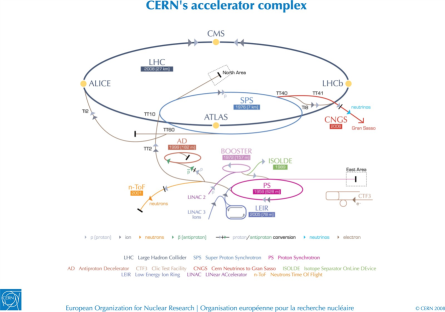
Figure 1: Overview of the CERN accelerator chain, showing the relationship between low-energy accelerators and the Large Hadron Collider with experiments. Image credit: CERN

The LHC itself is composed of two rings, one for each proton beam direction. Because the existing CERN tunnel has a diameter of just $3.7\,\mathrm{m}$, a “twin-bore” design first proposed by Blewett is used. In this design both rings are contained in a single superconducting cold mass and cryostat, but the magnetic dipole fields point in opposite directions to provide Lorentz bending force toward the center of the ring. An important part of the magnet design is the total dipole length of $15\,\mathrm{m}$, chosen to reduce the number of inter-cryostat connections.

The high magnetic field and large volume of these dipoles imply an enormous amount of stored magnetic energy in each magnet. A simple calculation per magnet of

$$E=\frac{1}{2}LI^{2}=\frac{1}{2}(0.099\,\mathrm{H})(11.8\,\mathrm{kA})^{2}=6.9\,\mathrm{MJ}$$ (1)

demonstrates the need for a quench protection system. The superconducting cable quenches and becomes a regular ohmic conductor if the temperature or magnetic field rise above critical values. If the current is not carried away through shunt resistances, it has the potential to boil off liquid helium explosively.

The protons beams themselves are accelerated with radio frequencies of 400 MHz, giving rise to synchroton oscillations that group protons into RF “buckets.” The collision rates in the interaction regions are proportional to $N_{\mathrm{p}}^{2}n_{b}$, where $N_{\mathrm{p}}$ is the number of protons per bunch and $n_{b}$ is the number of bunches. The LHC design goal is 2808 bunches. Within the beams, the proton population is distributed in both position space and momentum space, and the “emittance” is a measure of that spread. The longitudinal emittance relates to the bunch length, while the transverse emittance relates to the bunch (beam) width. The LHC beams are squeezed as they approach the interaction points, with the “strength” of the squeezing gradient given by $\beta^{\star}$. Formally, $\beta^{\star}$ is the distance from the interaction point where the beam width doubles, and a lower value of $\beta^{\star}$ means the beam is smaller at the interaction point. During early LHC operations a typical value of $\beta^{\star}$ has been $1.5\,\mathrm{m}$.

To calculate the expected rate of collisions in the LHC, we define the instantaneous luminosity $L$, measured in units of area^-1time^-1. Ultimately phase 1 of the LHC will reach instantaneous luminosities of $10^{34}\,\mathrm{cm}^{-2}\mathrm{s}^{-1}$ at full intensity. We can also write $L$ in units of cross section, using the definition $1\,\mathrm{barn}=10^{-24}\,\mathrm{cm}^{2}$ or $1\,\mathrm{nb}=10^{-33}\,\mathrm{cm}^{2}$, to estimate the rate of specific physics interactions. For example, with $L=10^{33}\,\mathrm{cm}^{-2}\mathrm{s}^{-1}=1\,\mathrm{nb}^{-1}\mathrm{s}^{-1}$ and inelastic proton-proton interaction cross section $\sigma=70\,\mathrm{mb}$ we expect a rate of $L\sigma=70\times 10^{6}$ interactions per second. Since the experiments collect data over an extended period of time, the integrated luminosity

$$\mathcal{L}=\int Ldt$$ (2)

is defined with units $\mathrm{area}^{-1}$, and then the dimensionless product $\mathcal{L}\sigma$ is the total number of interactions.

Exercise 1: Compare the center-of-mass energy in electron-positron collisions for (a) head-on collision of particles, each with energy $E_{\rm beam}$, and (b) collision of a beam particle with energy $E_{\rm beam}$ on a fixed target particle of mass $m_{e}$.

Exercise 2: Starting from the classical formula for the radiated power from an accelerated electron, show that the loss per turn due to synchrotron radiation is $\Delta E=4\pi e^{2}\gamma^{4}/3\rho$, where $\rho$ is the ring radius and $\gamma$ is the Lorentz factor of the electron.

3 Particle Detectors for the Energy Frontier

With the necessary beams designed and constructed to produce rare interactions sensitive to TeV-scale physics, we turn to the challenge of measuring the high-energy particles in the final states of those interactions. It is especially instructive to consider how particle detectors work from the point of view of the fundamental interactions. This allows us to predict how existing detectors would respond to new unusual particles in theories beyond the Standard Model.

In a nutshell, the ultimate goal of particle detection is to measure the 4-momentum of each final state particle. This can be accomplished by measuring $(p_{x},p_{y},p_{z},m)$, $(p_{x},p_{y},p_{z},E)$, or $(p_{T},\eta,\phi,E)$. This last form makes use of the definitions for transverse momentum $p_{T}^{2}=p_{x}^{2}+p_{y}^{2}$ and pseudorapidity $\eta=-\ln\left[\tan(\theta/2)\right]$. The relativistic momentum can be measured in a magnetic spectrometer, while the velocity in the lab frame can be measured in certain cases with precision timing circuits. Particle mass can be inferred from the energy loss through ionization, and the scalar energy can be measured in a shower of large cross section interactions.

It is clear that there must be some interaction of the final state particles with the detector medium, and we make use of the two highest-rate interactions – the electromagnetic and strong interactions. These two interactions affect the particles on two very different energy scales, since the electromagnetic interaction occurs on the atomic length scale (eV energy scale) and the strong interaction occurs on the nuclear length scale (GeV energy scale) [2].

A magnetic spectrometer is at the heart of every LHC experiment. The Lorentz force causes charged particles to move in helical trajectories in a solenoidal field. Measuring the sagitta of the projected helix gives a clean estimate of the particle’s transverse momentum, using the relation

$$s=\frac{0.3}{8}\frac{L^{2}B}{p_{T}}$$ (3)

where $L$ is the total arc length over which the sagitta is measured. In general, the uncertainty on the transverse momentum scales as $\sigma_{pT}/p_{T}\sim p_{T}$. Requirements on momentum resolution, dictated by physics goals, translate directly to requirements on sagitta resolutions. As an example, the ATLAS collaboration set a goal of 10% momentum resolution for $1\,\mathrm{TeV}$ muons expected from some new physics signatures. This implies a resolution of $50\,\mu\mathrm{m}$ on the sagitta measurement for trajectories that are nearly straight in the muon spectrometer. Increasing the magnetic field $B$ or the arc length $L$ (which is effectively the detector radius for straight tracks) increases the sagitta and leads to smaller relative uncertainties. This motivates large detectors like the ATLAS muon spectrometer, which has a maximum radius of $20\,\mathrm{m}$.

The interaction underlying most non-destructive measurements is the electromagnetic interaction, whether a particle scatters elastically off charges in material or loses energy through ionization of atomic electrons. In the former case, scattering from multiple charge centers results in an uncertainty on the particle’s original momentum vector. This uncertainty scales with the square root of the number of scatterers – $\left<\theta_{\mathrm{MS}}^{2}\right>=N\left<\theta^{2}\right>$, where $\theta$ is the deflection expected from a single scatter – and it is a powerful motivation for limiting the amount of material in the particles’ path. In the latter case, the energy loss follows the Bethe-Bloch formula, which in one form for a singly-charged particle looks like

$$\frac{dE}{d\rho x}\sim\left(\frac{N_{\mathrm{Avo}}Z}{A}\right)\left(\frac{\alpha^{2}\hbar}{m_{e}c}\right)\left(\frac{1}{\beta^{2}}\right)$$ (4)

This energy loss translates directly to a number of ionization electrons along the particle trajectory.

Charged particle detectors used controlled electric fields to collect ionization electrons and cations. In some cases, most notably in detectors with gaseous media, a central sense wire lies at the center of a radial electric field. As ionization electrons drift toward the center, the strongest part of the electric field, they are accelerated and induce an avalanche of additional ionization. This multiplication factor makes it possible to observe the passage of a particle in a relatively low-density medium. The position resolution of such detectors depends on exact knowledge of the drift time and is limited by placement accuracy of the central wires. Another detector type uses solid-state semiconductors, usually silicon, as the interaction medium. Particles passing through the semiconductor ionize valence electrons and create electron-hole pairs, which drift under an applied electric field to strip or pixel readout elements patterned on the surface. These detectors benefit from increased ionization energy loss (roughly $400\,\mathrm{keV/mm}$), but there is no amplification of collected charge, and special low-noise readout electronics are required to detect the signal. A major advantage of these detectors is that the readout element patterns can be microns apart, yielding extremely good position resolution. The disadvantages with respect to gaseous detectors are cost (gas is much cheaper than lithographed silicon) and processing requirements. Any defects in the semiconductor crystal trap the charge carriers and prevent them from reaching the readout elements. Because of their high cost and precision position resolution, solid-state detectors are most often placed near the interaction point, where they measure the first points of the particle trajectories before any scattering can take place.

By measuring the energy of a particle and either $\gamma$ or $\beta$, we can use the relation $E=\gamma m$ to determine the particle mass and therefore the particle type. Measurements of $\gamma$ and $\beta$ come from energy loss ($dE/dx$) as collected by readout electronics, direct velocity measurements via precision timing, or radiation emitted by charged particles in a dielectric medium (Cherenkov or transition radiation).

Energy measurements in calorimeters are by nature destructive measurements, since their aim is to fully contain and collect the energy of the incoming particle. There are two different mechanisms by which a particle entering the dense material of the calorimeter showers into a large number of second particles. The first mechanism, the electromagnetic shower, proceeds by alternating electron bremsstrahlung to photons and subsequent conversion to electron-positron pairs. Only photons and electrons participate in the electromagnetic shower, since both bremsstrahlung and pair production are maximized for low mass particles. The second mechanism, the hadronic shower, is due to nuclear interactions. For both mechanisms, the cascade undergoes exponential branching until the energy of individual particles falls below some critical energy and ionization takes over.

Because of the exponential growth of the shower, the total number of secondary particles is proportional to the energy of the primary particle that entered the calorimeter. The energy resolution of the calorimeter, then, is given by

$$\frac{\sigma_{E}}{E}\sim\frac{\sigma_{N}}{N}\sim\frac{1}{\sqrt{E}}$$ (5)

since the fluctuations in the large number of particles follow a Gaussian distribution. The secondary particles in the shower can be collected in a dedicated active medium distinct from the absorber material (as in a non-homogeneous calorimeter) or in the same medium that serves as absorber (in a homogeneous calorimeter). This distinction has a substantial effect on the energy resolution; for example, the electromagnetic energy resolution is $\sigma_{E}/E=10\%/\sqrt{E}$ in ATLAS but $2.7\%/\sqrt{E}$ in CMS. In the LHC experiments, two distinct calorimeters are deployed, one representing a small number of nuclear interaction lengths but large number of electromagnetic radiation lengths, and one with a large number of nuclear interaction lengths. These are the electromagnetic and hadronic calorimeters, respectively.

Particles that do not interact strongly, such as muons and neutrinos, penetrate the calorimeters without showering. Muons are detected in standalone external spectrometers or chambers integrated in the magnet yoke. Neutrinos do not interact with any of the detector material, and any missing momentum in the collision is attributed to them. Figure 2 shows in detail the experimental signature of the Standard Model particles, as detected in the CMS experiment.

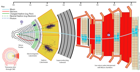
Figure 2: Transverse slice through the CMS detector, showing the individual detector subsystems and particle signatures in each. The particle type can be inferred by combining the detector response in the different subdetectors. Image credit: CERN

The high interaction rates required to search for new physics at the TeV scale present extra challenges for the LHC experiments. Charged particle tracking algorithms are designed to function with detector occupancies of up to $\mathcal{O}(1\%)$. These algorithms, which work by stringing together significant energy deposits (“hits”), start with the highest-granularity silicon detectors near the interaction point and work outward, accounting for energy loss in each detector layer encountered. The experiments have been designed to meet the requirements of low occupancy even in particle-dense environments like boosted jets from high-mass resonances or Higgs boson decays.

Certain examples of physics beyond the Standard model give rise to striking experimental signatures, and it is worth looking at a few such examples. First, exotic charged massive particles (CHAMPs) typically have low velocities, with $\beta$ significantly less than 1. This causes them to lose greater amounts of energy through ionization, and they may even stop in the middle of the detector if the energy loss is great enough. Since the particles are massive they do not shower in the electromagnetic calorimeter. R-hadrons, stable particles with heavy colored constituents, can have similar signatures. Doubly-charged particles lose $q^{2}=4$ times the normal ionization energy loss in the tracking detectors, a unique signature for any experiment with $dE/dx$ sensitivity. Second, metastable particles, such as long-lived neutralinos in theories of supersymmetry breaking, may have $c\tau$ values of order $1\,\mathrm{m}$, and the decay products do not point back to the primary interaction vertex. Even though it is challenging to reconstruct particles originating in the middle of the detector, successful reconstruction makes it possible to measure the lifetime of the parent particle. Third, exotic “quirks,” predicted in new theories of strong interactions, can appear as a mesoscopic bound state, with properties similar to a doubly-charged particle, or as a state that oscillates like a macroscopic string with two charge endpoint particles.

These and other particle interactions can be modeled with dedicated computer programs of differing complexity. On one end lies GEANT4 [3, 4], a simulation toolkit with detailed lists of high- and low-energy interactions. Each particle is tracked step-by-step through a custom model of the detector. On the other end lie fast simulation programs like PGS [5] and Delphes [6], which use parameterized detector response to each type of particle.

Careful consideration of the physical interactions behind the experimental techniques allows one to extrapolate detector behavior to the most unusual new possibilities! Unfortunately experiments do not have large enough computing budgets to store the detector response to each bunch crossing, so they use a multi-level trigger system to decide immediately which events should be saved. This bears repeating: unless the new physics is selected by a trigger algorithm, it will be lost forever.

The LHC experiments use a combination of low-level hardware and high-level software triggers to filter events for further study. In the hardware triggers, individual trigger objects (jets, electromagnetic clusters, muons) are identified using data from fast readout detectors. These are passed to streamlined versions of offline software algorithms to be reconstructed more fully. For example, an electron trigger might require a Level-1 electromagnetic cluster with $E_{T}>20\,\mathrm{GeV}$, followed in the High-Level Trigger with a set of track-matching requirements and further cluster shape cuts to reject jets and $\pi^{0}$ mesons. If the rate of electron events becomes too great, then some filter has to be tightened to reduce the overall rate.

Exercise 3: Beginning from the Lorentz force law, prove the relation in Eqn. 3 between the sagitta and transverse momentum of a charged particle.

Exercise 4: In silicon strip detector with strip pitch (spacing) $d$, a hit on a strip means a particle passed somewhere in the $\{-d/2,+d/2\}$ range centered on the strip. Show that the variance of this uniform distribution is the same as that of a Gaussian distribution with width $d/\sqrt{12}$.

4 Physics Studies with Hadronic Jets

Many Standard Model and new physics signatures include hadronic jets. These jets present many challenges for the LHC experiments, and since they are the result of peturbative and non-perturbative QCD effects they also test our theoretical framework. Because the jets are measured chiefly in the calorimeters, experimentalists develop special energy calibrations to account for the effects of hadronization and contributions from pileup.

Even though we do not expect a one-to-one correspondence between reconstructed jets and partons (except possibly for the highest energy partons) we do expect that the relation between the two should be calculable on average. In the past decade experimentalists have become more sophisticated in defining jets and comparing measurements with theoretical predictions. Such comparisons are always made at the “particle-level” or “hadron-level,” after the parton shower and hadronization but before the detector interaction occurs. This means that theoretical predictions must apply a showering and hadronization model to parton-level results, and experiments must unfold the effects of jet reconstruction in the detectors.

We have first to define exactly what is meant by “jets,” and there are three main considerations. First, what particles should be clustered, or what inputs will be given to the algorithms? Second, which particles should be combined into each jet, based on proximity and energy? Third, how should the input 4-momenta be combined? The goal is to define jet clustering algorithms that are fast, robust under particle boosts, and able to deal with collinear and infrared radiation. This problem has been studied in great detail [7], but it is useful to summarize some of the solutions.

The answer to the first question is that the inputs can in fact be any kind of 4-momentum, possibly associated with truth particles (to give truth jets) or calorimeter cells (reconstructed jets). The answer to the third question seems to have been decided in favor of adding 4-momenta vectorially. There are many answers to the second question of how to choose the particles to combine into each jet!

Perhaps the simplest way to cluster particles is to use a cone algorithm, in which a distance $\Delta=\sqrt{(\Delta\eta)^{2}+(\Delta\phi)^{2}}$ is defined with respect to a seed particle (typically the highest-$p_{T}$ particle). All particles satisfying $d<R$ lie in a circle of radius $R$ in the $\eta-\phi$ plane of the calorimeter, and these particles are combined to form a jet 4-momentum. This algorithm is well-defined geometrically, but the choice of seed particle is not stable when collinear radiation is considered.

A more sophisticated class of algorithms combine nearest particles first, effectively reversing the branching of the parton shower, instead of fixing a seed particle and cone. These “sequential recombination” algorithms cluster particles with smallest $d_{ij}$ first, where

$$d_{ij}=\min\left(k_{ti}^{2p},k_{tj}^{2p}\right)\frac{\Delta_{ij}^{2}}{R^{2}}$$ (6)

for particles $i,j$ and beam 4-vector $t$. (Particles whose closest neighbor is the beam are considered stable jets.) In this general formulation, different values of the exponent $p$ give very different algorithms. For $p=0$ (Cambridge-Aachen algorithm), particles near each other in $\eta,\phi$ coordinate space are clustered first, whereas for $p=1$ (kT algorithm) lower-momentum particles are clustered first.

Cacciari et al. pointed out recently that the case $p=-1$ also defines a useful algorithm, the anti-kT algorithm [8]. This choice means that the particles around the hardest particle are clustered first. The anti-kT algorithm guarantees a cone-like geometry with well-defined jet borders around the highest momentum particles (see Fig. 3), but it maintains the infrared safety and collinear safety of the sequential recombination family. This algorithm has become a preferred jet algorithm for LHC experiments, along with a modified stable infrared-safe cone algorithm called SISCone [9].

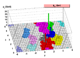
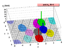
Figure 3: Comparison of jet catchment areas for two different jet clustering algorithms[8]. All particles within a jet’s catchment area will be clustered into the jet.

Total energy measured for a jet at the detector level must be corrected to match the energy at the particle level, and the calibration of the jet energy scale is a major experimental uncertainty in signatures with hadronic jets [10]. In short, the following effects are included in the calibration: varying detector response due to non-linearities or uninstrumented regions, mixed electromagnetic and hadronic showers in the same calorimeter, overall absolute energy scale calibration (assuming differences in relative response have been treated), and loss or gain of particles in the region defined by the jet area. These effects are estimated using calibration data samples in the jet-jet or $\gamma$+jet signatures, where the true jet energy can be estimated from the other object’s recoil. Because there are no sufficiently large data samples of jets at the highest energies, jet calibration at those energies is based on extrapolation or on Monte Carlo simulation.

Certain jets, specifically those associated with heavy quarks ($b,c$), have several special properties due to the quarks themselves. The heavy quarks stand out for their long lifetimes (due to CKM suppression), large mass with respect to their decay products, and high multiplicity decays. These properties give rise to a distinct decay geometry, shown in Fig. 4. The momentum vectors of decay products from the $B$ point to a secondary vertex, not the primary interaction vertex, and the distance between the two vertices depends on the $b$ lifetime, if we use the spectator model approximation for the decay of the heavy quark hadron. Typical values before boost factors are $c\tau_{b}=500\,\mu\mathrm{m}$, $c\tau_{c}=500\,\mu\mathrm{m}$, and $c\tau_{\tau}=90\,\mu\mathrm{m}$. Because finding a common vertex for two or more tracks is one of the most challenging problems in tracking, the impact parameter of a track is used as a proxy to determine if it is consistent with having come from the primary interaction vertex. If a large number of tracks in a jet are inconsistent with the primary vertex, then it is likely that there is a heavy flavor hadron in the jet. One of the primary motivations for developing precision solid-state tracking detectors, which are even sometimes named “vertex detectors,” is to measure track parameters precisely enough to allow for vertexing. The same parameters are also use for exact impact parameter measurements with 10% precision on values of $\mathcal{O}(300\,\mu\mathrm{m})$.

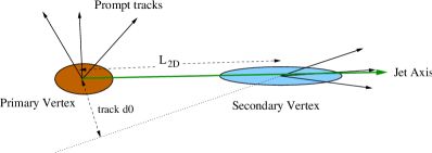
Figure 4: Displaced secondary vertex from decay of a long-lived particle. Tracks from the decay are not expected to point back to the primary vertex as prompt tracks do. Flavor tagging (b-tagging) algorithms are designed to identify tracks with significant impact parameter $d_{0}$ and a vertex with significant decay length $L_{2D}$.

Flavor tagging algorithms are not limited to decay lengths and impact parameters. Identifying medium-$p_{T}$ leptons from semileptonic heavy flavor decays provides an independent tagging mechanism. Since charm quarks also have long lifetimes and semileptonic decays, we use discriminating variables based on the mass of all particles in the secondary vertex to distinguish $b$-jets from $c$-jets. Ultimately, multivariate techniques combine information from all of these measurements to give powerful separation between $b$, $c$ and light quark jets. Tighter requirements on $b$-jets reduce $c$ and light quark jet contamination but also reduce the $b$-tagging efficiency, as shown in Fig. 5.

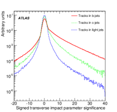
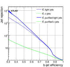
Figure 5: Impact parameter significance distribution (left) and flavor tagging peformance (right) from the ATLAS experiment [11]. Flavor tagging algorithms exploit the difference in the impact parameter distributions to select jets from bottom quarks while rejecting jets from light quarks ($u,d,s$) and, to a lesser extent, jets from charm quarks.

In the Standard Model, the proton-proton collision at a fixed center-of-mass energy is in fact a parton-parton collision between partons of unknown energy. As a result, the longitudinal momentum of the initial state is completely unknown, and this complicates the final state reconstruction. The key is to realize that the initial transverse momentum is well known; it is essentially 0 because of the small horizontal emittance of the beams and the low energy scale of $\Lambda_{\mathrm{QCD}}$. The final state transverse momentum is expected therefore to also equal 0, and any deviation can be interpreted as missing transverse momentum or “missing transverse energy” ($E_{T}^{\mathrm{miss}}$ or MET), presumably due to non-interacting particles produced in the interaction but not detected.

The LHC experiments define the missing transverse energy as the opposite of the vector transverse sum of all detected particles. Such a measurement is only relevant if the detectors are nearly hermetic to both charged and neutral particles; this has put strict requirements on the hermeticity of the experiments. Corrections are applied for the detector response to muons and jets, and in some cases information from tracking and calorimetry is combined to optimize the missing energy reconstruction. The missing energy scale and resolution are calibrated using events known to have specific missing energy, e.g., $Z(\rightarrow\nu\bar{\nu})$+jets events. It is important to calibrate several different points to enable extrapolation to the higher values of $E_{T}^{\mathrm{miss}}$ we expect in new physics signatures. Like all energy measurements, the absolute resolution on the missing transverse energy scales as $\sqrt{E}$; early measurements of the ATLAS resolution yielded $\sigma=0.57\sqrt{E\,(\mathrm{GeV})}$.

Exercise 5: The cone algorithm for jet clustering has its drawbacks, but it does have one redeeming quality. Use the definition of the pseudorapidity $\eta$ to show that a cone size of $\Delta R\equiv\sqrt{(\Delta\eta)^{2}+(\Delta\phi)^{2}}$ is invariant under boosts along $\hat{z}$.

Exercise 6: Use Fig. 4 to show that, for a typical track from a $B$ hadron decay, $d_{0}\sim(c\tau_{B})$, assuming the kick transverse to the jet axis is due to the large mass of the $B$ hadron. Hint: consider the angle $\theta$ the track makes with respect to the $b$-jet axis. (This relation shows that the $B$ mass is not as important as the lifetime when we consider track impact parameters, and it explains why tracks from charm decay have $d_{0}$ values of similar magnitude.)

5 Searches for Higgs Bosons

The search for the Higgs boson, whether in the Standard Model or beyond, is a key goal for understanding the physics of the terascale. The $W$ and $Z$ boson and $t$ quark masses near the $100\,\mathrm{GeV}$ scale give quantitative constraints on the Standard Model Higgs boson mass, the only unknown parameter in the electroweak sector. In particular, precision measurements of $m_{W},m_{Z},m_{t}$ constrain Higgs loop contributions and favor low Higgs masses, below $200\,\mathrm{GeV}$. Direct experimental searches at LEP and Tevatron rule out $m_{H}<114\,\mathrm{GeV}$ and $158<m_{H}<175\,\mathrm{GeV}$, respectively [12, 13].

Standard Model Higgs boson production cross sections and branching ratios depend only on the Higgs mass. As seen in Fig. 6, the gluon fusion production mechanism dominates, but other production mechanisms are important for signatures with small background contributions. The branching fractions change quickly with increasing $m_{H}$ as phase space for new decay channels opens. One notable feature is the dominant $WW$ decay even above $2m_{Z}$; this is explained by the Standard Model Lagrangian term

$$\mathcal{L}\sim(2M_{W}^{2}HW_{\mu}^{+}W^{-\mu}+M_{Z}^{2}HZ_{\mu}Z^{\mu}).$$ (7)

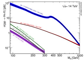
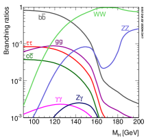
Figure 6: Calculations of the Standard Model Higgs boson production $pp$ cross section (left) and branching fractions (right) [14].

A successful Higgs boson search would show not only a discrepancy in the data with respect to the Standard Model prediction (without Higgs), but also consistency with expected Higgs production. We choose a specific experimental signature or “channel” and develop an event selection to reject backgrounds from SM physics processes. The data sample may include contributions from background processes and putative signal events, but the goal is to measure the background contributions directly from data, if possible, to avoid any bias or errors in simulation.

A vital, if controversial, part of the Higgs search is the statistical interpretation of observed results in the context of a Higgs boson production hypothesis. What is the probability that the observed dataset is consistent with background-only production? With signal plus background production? Suppose 40 background (SM) events are expected in a search for a model that predicts 10 events from a new physics signal. Can the new physics model be excluded definitively if 40 events are observed? Can the Standard Model be excluded if 50 events, or even 60 events, are observed?

Much work in the past decade has focused on bringing sophisticated statistical tools to bear on this question in particle physics. The most common shorthand for presenting results is a re-interpretation in terms of a Gaussian distribution. If the observed experiment is considered as one of many possible experiments, given a certain model, then it is possible to calculate where the observed experiment lies in the distribution of the “pseudo-experiments” and convert its percentile to a number of “sigma.” That is, if $\alpha$ is the probability to measure a less likely value than the observed experiment, then $\alpha=0.3173$ corresponds to a $1\sigma$ deviation. (It is important to be aware of the distinction, sometimes overlooked, between one-sided and two-sided definitions of $\alpha$ [15]. Two-sided definitions are typical for measurements, while one-sided is often used for counting events when the signal is unknown.)

Usually we are interested in testing two complementary hypotheses, that of background-only production ($s=0$) and that of signal+background production ($s>0$). If the data favor the latter hypothesis and strongly disfavor the former, then we have a discovery. Experiments often report results in terms of a likelihood ratio $LR=L_{s+b}/L_{b}$ and by asking the following: how often can certain values of the LR be expected from an experiment in the presence of signal? For a discovery we talk about excluding the background hypothesis at $>5\sigma$, which is $P_{b}<10^{-7}$.

Most of the progress in the past five years has been on the treatment of systematic uncertainties, which reflect the inherent uncertainty in the number of background and signal expected in the datasets. Poorly constrained backgrounds can doom a Higgs search just as surely as low integrated luminosity. An overview of some methods, with technical results somewhat beyond the scope of these lectures, is given in Ref. [16].

Now it is instructive to introduce four of the main Standard Model Higgs boson searches at the LHC and to have a peek at one that may be important in the future.

For low mass Higgs bosons ($m_{H}<130\,\mathrm{GeV}$), one might expect to search for Higgs resonances produced in gluon fusion and decaying to $b\bar{b}$ pairs. Unfortunately, non-resonant $gg\rightarrow b\bar{b}$ production has an enormous production rate at the LHC, about 6 orders of magnitude greater than Higgs production! Fortunately, there are two other possibilities.

Higgs decays to tau lepton pairs (approximately 10% branching fraction) do not suffer from the $gg$ background because the tau is not colored. The dominant background process is $Z\rightarrow\tau^{+}\tau^{-}$, but the $Z$ mass resonance is well below the search region. After two tau lepton candidates have been reconstructed in an event, using algorithms that identify fully leptonic decay or hadronic decay, the missing transverse energy is used to estimate the energy taken by two or more neutrinos. With no other information, the kinematic system would be underconstrained, and mass reconstruction of the $\tau\tau$ system would be impossible. If one assumes the tau leptons from Higgs decays are highly boosted, then the neutrinos in the tau decay all have the same momentum as their sister decay products. With this trick, it is possible to reconstruct the full tau momentum and calculate the invariant mass of the Higgs candidate (see Exercise 8).

Higgs decays to two photons are a tiny fraction of all decays, but there are no diphoton resonances in the Standard Model above $1\,\mathrm{GeV}$, so any sign of a resonance would be a clear indication of new physics. The LHC experiments, particularly ATLAS and CMS, have been designed to have excellent resolution for both photon energy and direction, and significant effort has gone into rejecting fake photons (misidentified electrons or jets) to reduce background. The non-resonant diphoton background can be measured as a falling distribution in data, as shown in Fig. 7 compared to the signal expectations for Standard Model Higgs production. This search is limited only by the number of events that can be collected, given the small branching ratio.

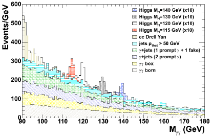
Figure 7: Invariant mass spectrum of diphoton candidates selected in the low-mass Higgs boson search [17]. The significance of the diphoton resonances depends on the mass resolution of the experiment and the level of background underneath the signal peak.

For high mass Higgs bosons ($m_{H}>170\,\mathrm{GeV}$), the $ZZ\rightarrow\ell^{+}\ell^{-}\ell^{+}\ell^{-}$ decay channel offers another clean signature. Even though there is non-resonant $ZZ$ Standard Model production, the reconstructed Higgs resonance would stand out clearly, as shown in Fig. 8. Again, the LHC experiments are designed to make precise measurements of the high-$p_{T}$ electrons and muons, even for large Higgs masses; this defines the target resolution for the muon spectrometers.

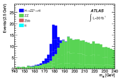
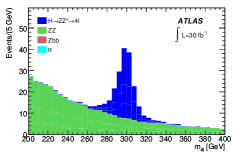
Figure 8: Reconstructed 4-lepton mass for signal and background processes, assuming $m_{H}=180\,\mathrm{GeV}$ (left) and $m_{H}=300\,\mathrm{GeV}$ (right) [11].

For medium mass Higgs bosons ($130<m_{H}<170\,\mathrm{GeV}$), the dominant decay is $H\rightarrow W^{+}W^{-}$. This signal process has a large rate using all production mechanisms, and the decay to a dilepton signature is clean. There are two challenges for searches in this channel. First, the presence of two high-$p_{T}$ neutrinos means there is no invariant mass peak for the reconstructed Higgs. (Since the $W$ bosons are not boosted, the reconstruction trick from the tau channel cannot be re-used.) Second, direct $WW$ production and top quark pairs have similar dilepton+$E_{T}^{\mathrm{miss}}$ signatures, but even here there is one extra trick for selecting $WW$ pairs from Higgs decay. Because the Higgs is a scalar boson with spin 0, the two $W$ bosons from Higgs decay must have opposite spin, and the leptons from $W$ decay tend to be closer in direction than in the $t\bar{t}$ case. The angle between leptons is one of several input variables for multivariate tools that separate Higgs signal from SM background. This technique has already been used at the Tevatron to exclude certain Higgs mass hypotheses between 158 and 175 GeV [13].

The peek into the future regards the dominant $b\bar{b}$ decay channel for low-mass Higgs bosons. Since electroweak fits favor low Higgs masses, this decay channel would seem to be of prime importance in the Higgs search, but the $b\bar{b}$ jet background limits its sensitivity. (If the $b\bar{b}$ mass resolution were as good as the $\gamma\gamma$, a peak might still be resolved, but the jet energy resolution is limited by fluctuations in the hadronic shower.) One way to reduce the $b\bar{b}$ background is to require associated production of $W,Z$ or $t\bar{t}$, and all of these associated production channels are being studied. A novel idea focuses the $WH/ZH$ search to the region of phase space where the vector boson has large transverse momentum. Events in this region have a highly-boosted Higgs boson and $b\bar{b}$ decay products observed in a single fat jet. By shrinking the jet clustering radius until the two $b$ subjets are resolved (as in Fig. 9), it is possible to compare the masses of the subjets to the mass of the boosted Higgs jet[18]. The large mass drop from the parent Higgs jet to both daughter $b$ subjets is nearly unique; only the $WZ$ decay to $b\bar{b}$ has a similar reduction. The background from two-body $gg\rightarrow b\bar{b}$ decay is greatly reduced, and the dominant background becomes $W/Z$+light jet production. The benchmark calibration for this new technique is the reconstruction of the $Z$ peak in Standard Model $WZ$ and $ZZ$ production.

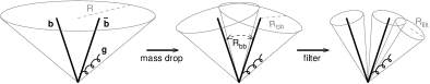
Figure 9: Description of jet algorithm to identify boosted jets and substructure within [18]. The algorithm is designed to identify cleanly two $b$-jets from $H\rightarrow b\bar{b}$ decay, but it can be used for any decay of a particle to products having much lower mass.

Because the Higgs production cross section is small, several promising channels must be combined in the low-mass region to ensure sensitivity. When added to the powerful high-mass channels ($WW,ZZ$), these searches guarantee the LHC experiments will have something definitive to say about the Standard Model Higgs boson in the near future, perhaps with several $\mathrm{fb}^{-1}$ of 7 TeV data.

Exercise 7: There is a quick way to estimate the “number of sigma” significance of a signal observed above the background expectation. Use Poisson probabilities to define a likelihood ratio $L=P_{s+b}/P_{b}$ and show that to good approximation

$$\sigma\equiv\sqrt{2\ln L}=\sqrt{2\left[\left(s+b\right)\ln\left(1+\frac{s}{b}\right)-s\right]},$$

where $s$ and $b$ are the expected numbers of signal and background events, respectively.

Exercise 8: (suggested by M. Strassler): Consider an event $pp\rightarrow Z+\gamma$, where the $Z$ decays to $\tau^{+}\tau^{-}$. Use the fact that, although the neutrinos carry off energy, they do not significantly alter the directions of the tau leptons’ other decay products, since the taus are highly boosted. Show that the $Z$ boson mass can be reconstructed using only the photon momentum, the observed missing $p_{T}$ , and the tau momentum directions (not their energies). This technique can also be used to measure the Higgs boson mass in $H\rightarrow\tau^{+}\tau^{-}$ decays.

6 Searches for Physics beyond the Standard Model

Searches for physics beyond the Standard Model (BSM) follow one of two approaches. The search strategy may focus on a specific model, or it may target any discrepancy from the Standard Model expectation. Both of the strategies are used in the LHC experiments, which hunt for general features in data that may correspond to a wide range of BSM models. Results in this section are a sampling of techniques used in new physics searches.

Perhaps the most straightforward signature shared by BSM models is the total event energy. New physics related to the terascale often has energies near this scale. The outgoing events in the hard scatter set the event scale, which is near the mass of the heavy new particles. Whatever the exact nature of their subsequent decay, the event energy scale is roughly preserved. As a result, the total event energy is a good estimate for the mass of new particles produced in pairs. To make this connection, it is best to focus on a robust definition of the total events energy.

There are at least three common calculations corresponding to total event energy. The first is the simple $\sum E_{T}$, for which all calorimeter energy is summed. This definition does not cover non-interacting particles, such as neutrinos or weakly interacting massive particles, nor does it account for extra calorimeter activity due to pileup events. The second is the oft-misunderstood $H_{T}$, usually defined as the scalar sum of missing transverse energy and the transverse energies of identified jets and leptons. This definition works well if there are one or two non-interacting particles, but it still suffers from pileup contamination and depends on the identification of the physics objects. The third is the effective mass $M_{\mathrm{eff}}$, usually defined as the scalar sum of transverse energies of the four hardest identified jets and the missing transverse energy. This definition suppresses low-energy contributions from pileup events, but it does not capture the leptonic parts of the new particles decay chains. All three of these definitions are used in various channels by the LHC experiments, where they show good discriminating power between Standard Model background and the new physics signal.

Many arguments have been advanced for higher-mass versions of SM particles, and some of these correspond to resonances (invariant mass peaks) of simple objects, such as leptons or jets. Examples include Kaluza-Klein towers of particles confined in extra dimensions, $Z^{\prime}/W^{\prime}$, and $t^{\prime}$, a 4th-generation up-type quark. Reconstruction of these resonances is straightforward, if the 4-momenta of all decay objects are known. The sensitivity to resonances is limited by background contamination and invariant mass resolution, both of which are high priorities for the LHC experiments.

If some of the decay products from the new resonance are invisible (non-interacting), a simple invariant mass calculation will not capture the signal. In these cases, the transverse mass

$$m_{T}^{2}=2E_{T1}E_{T2}\left[1-\cos(\Delta\phi)\right]$$ (8)

can be used, using as $E_{T}$ the missing transverse energy. If two particles decay to invisible daughters, as in cascade decay chains to lightest supersymmetric particles, it is still possible to apportion correctly the missing transverse energy. For example, in the supersymmetric decay chain

$$pp\rightarrow X+\tilde{\ell}^{+}_{R}\tilde{\ell}^{-}_{R}\rightarrow X+\ell^{+}\ell^{-}\chi_{1}^{0}\chi_{1}^{0}$$ (9)

the final state neutralinos both appear as missing transverse energy. If the $\chi_{1}^{0}$ mass is known, then the mass equivalence of the slepton mothers gives enough constraints to construct a kinematic variable whose distribution endpoint gives the slepton mass [19].

For a more concrete example, consider the following decay in theories of gauge-mediated supersymmetry breaking:

$$\tilde{\chi}_{2}^{0}\rightarrow\tilde{\ell}^{\pm}\ell^{\mp}\rightarrow\tilde{\chi_{1}^{0}}\ell^{\mp}\ell^{\pm}\rightarrow\tilde{G}\gamma\ell^{\pm}\ell^{\mp}$$ (10)

Assuming that the background in this dilepton channel can be estimated using an opposite-flavor sample, the background-subtracted invariant mass distribution (Fig. 10) shows a sharp edge, indicating a kinematic limit [20]. In this case, the location of the edge is determined by the relation between the neutralino and slepton masses. The minimum mass for the $\ell\ell\gamma$ system has a similar endpoint, given by the difference of the neutralino masses. By using these and other kinematic solution endpoints, it is possible to reconstruct all of the masses in the decay chain.

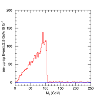
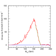
Figure 10: Invariant dilepton mass distribution (left) and minimum dilepton+photon mass distribution (right) with background subtraction for GMSB signal events [20]. The endpoints of the background-subtracted distributions can be used to determine the masses of intermediate particles in the new physics decay chain. These figures represent data corresponding to an integrated luminosity of $10\,\mathrm{fb}^{-1}$.

An alternative to targeted searches has emerged in the last decade. Instead of developing event selections and kinematic variables designed for each of many different models and decay chains, some experiments have deployed general search strategies. These programs, count events in each of several high-$p_{T}$ object classes ($1\mu 1\mathrm{jet},1e2\mathrm{jet}$, etc.) and compare the results to SM expectations [21, 22, 23]. The challenge is to describe completely the SM backgrounds for all signatures at once! Several discriminant distributions are considered for each class, including the scalar $p_{T}$ sum of all objects, the invariant mass (or transverse mass) of all objects, and the missing transverse energy. Any discrepancies between observed data and expectations are flagged for further studies.

In conjunction with the rise in general searches, new emphasis has been placed on simplified phenomenological models, which include the gross effects of new particle mass spectra and decay chains without focusing on the details of particle couplings and spin effects. These models have been successful in identifying experimental signatures that may have been overlooked [24], and they offer hope of helping match experimental observations with consistent theoretical models of new physics [25].

7 Conclusion

The Large Hadron Collider and associated experiments have been designed and constructed to answer questions about physics at the 1 TeV scale. The size, scope, and details of the experiments stem directly from the physics goals and requirements on measurements at that energy scale.

The focus in the last few sections on Higgs boson searches and other specific searches led naturally to a concentration on results from the general-purpose ATLAS and CMS experiments, but the other LHC experiments have been designed to pursue different physics goals that are no less interesting. All of the detector interactions, many of the design considerations, and some of the analysis techniques are being brought to bear on those goals as well.

A basic understanding of detector physics and practical limitations makes interpretation of experimental results more exciting and engaging, and the next few years may even bring news of exotic new particles with unexpected signatures.

References

- [1] E. Eichten, I. Hinchliffe, K. D. Lane, and C. Quigg, “Super Collider Physics,” Rev. Mod. Phys. 56 (1984) 579–707.
- [2] D. Green, The Physics of Particle Detectors. Cambridge University Press, Cambridge, 2000.
- [3] GEANT4 Collaboration, S. Agostinelli et al., “GEANT4: A Simulation toolkit,” Nucl.Instrum.Meth. A506 (2003) 250–303.
- [4] J. Allison, K. Amako, J. Apostolakis, H. Araujo, P. Dubois, et al., “Geant4 developments and applications,” IEEE Trans.Nucl.Sci. 53 (2006) 270.
- [5] J. Conway, PGS4: Pretty Good Simulation of high energy collisions, 2009. http://physics.ucdavis.edu/~conway/research/software/pgs/pgs4-general.h%tm.
- [6] S. Ovyn, X. Rouby, and V. Lemaitre, “DELPHES, a framework for fast simulation of a generic collider experiment,” arXiv:0903.2225 [hep-ph].
- [7] G. C. Blazey et al., “Run II jet physics,” arXiv:hep-ex/0005012.
- [8] M. Cacciari, G. P. Salam, and G. Soyez, “The anti-k_t jet clustering algorithm,” JHEP 04 (2008) 063, arXiv:0802.1189 [hep-ph].
- [9] G. P. Salam and G. Soyez, “A practical Seedless Infrared-Safe Cone jet algorithm,” JHEP 05 (2007) 086, arXiv:0704.0292 [hep-ph].
- [10] CDF Collaboration, A. Bhatti et al., “Determination of the jet energy scale at the collider detector at Fermilab,” Nucl. Instrum. Meth. A566 (2006) 375–412, arXiv:hep-ex/0510047.
- [11] ATLAS Collaboration, G. Aad et al., Expected Performance of the ATLAS Experiment - Detector, Trigger and Physics. CERN, Geneva, 2009. arXiv:0901.0512.
- [12] R. Barate et al., “Search for the standard model Higgs boson at LEP,” Phys. Lett. B565 (2003) 61–75, arXiv:hep-ex/0306033.
- [13] Tevatron New Physics and Higgs Working Group, “Combined CDF and D0 Upper Limits on Standard Model Higgs- Boson Production with up to 6.7 fb-1 of Data,” arXiv:1007.4587 [hep-ex].
- [14] LHC Higgs Cross Section Working Group, S. Dittmaier, C. Mariotti, G. Passarino, and R. Tanaka (Eds.), “Handbook of LHC Higgs Cross Sections: 1. Inclusive Observables,” arXiv:1101.0593 [hep-ph].
- [15] Particle Data Group Collaboration, K. Nakamura et al., “Review of particle physics,” J.Phys.G G37 (2010) 075021.
- [16] E. Gross, “LHC Statistics for Pedestrians,” in PHYSTAT-LHC Workshop on Statistical Issues for LHC Physics, L. Lyons, H. Prosper, and A. de Roeck, eds., pp. 205–212. CERN, Geneva, 2008. http://doc.cern.ch/yellowrep/2008/2008-001/p205.pdf.
- [17] CMS Collaboration, G. Bayatian et al., “CMS physics technical design report, Volume II: Physics performance,” Journal of Physics G: Nuclear and Particle Physics 34 no. 6, (2007) 995.
- [18] J. M. Butterworth, A. R. Davison, M. Rubin, and G. P. Salam, “Jet substructure as a new Higgs search channel at the LHC,” Phys. Rev. Lett. 100 (2008) 242001, arXiv:0802.2470 [hep-ph].
- [19] C. G. Lester and D. J. Summers, “Measuring masses of semiinvisibly decaying particles pair produced at hadron colliders,” Phys. Lett. B463 (1999) 99–103, arXiv:hep-ph/9906349.
- [20] I. Hinchliffe and F. E. Paige, “Measurements in gauge mediated SUSY breaking models at LHC,” Phys. Rev. D60 (1999) 095002, arXiv:hep-ph/9812233.
- [21] D0 Collaboration, B. Abbott et al., “Search for new physics in e muon X data at D0 using Sleuth: A Quasi model independent search strategy for new physics,” Phys. Rev. D62 (2000) 092004, arXiv:hep-ex/0006011.
- [22] H1 Collaboration, A. Aktas et al., “A general search for new phenomena in e p scattering at HERA,” Phys. Lett. B602 (2004) 14–30, arXiv:hep-ex/0408044.
- [23] CDF Collaboration, T. Aaltonen et al., “Model-Independent and Quasi-Model-Independent Search for New Physics at CDF,” Phys. Rev. D78 (2008) 012002, arXiv:0712.1311 [hep-ex].
- [24] D. Alves et al., “Simplified Models for LHC New Physics Searches,” arXiv:1105.2838 [hep-ph].
- [25] N. Arkani-Hamed et al., “MARMOSET: The Path from LHC Data to the New Standard Model via On-Shell Effective Theories,” arXiv:hep-ph/0703088.