Eliciting Forecasts from Self-interested Experts: Scoring Rules for Decision Makers

Abstract

Scoring rules for eliciting expert predictions of random variables are usually developed assuming that experts derive utility only from the quality of their predictions (e.g., score awarded by the rule, or payoff in a prediction market). We study a more realistic setting in which (a) the principal is a decision maker and will take a decision based on the expert’s prediction; and (b) the expert has an inherent interest in the decision. For example, in a corporate decision market, the expert may derive different levels of utility from the actions taken by her manager. As a consequence the expert will usually have an incentive to misreport her forecast to influence the choice of the decision maker if typical scoring rules are used. We develop a general model for this setting and introduce the concept of a compensation rule. When combined with the expert’s inherent utility for decisions, a compensation rule induces a net scoring rule that behaves like a normal scoring rule. Assuming full knowledge of expert utility, we provide a complete characterization of all (strictly) proper compensation rules. We then analyze the situation where the expert’s utility function is not fully known to the decision maker. We show bounds on: (a) expert incentive to misreport; (b) the degree to which an expert will misreport; and (c) decision maker loss in utility due to such uncertainty. These bounds depend in natural ways on the degree of uncertainty, the local degree of convexity of net scoring function, and natural properties of the decision maker’s utility function. They also suggest optimization procedures for the design of compensation rules. Finally, we briefly discuss the use of compensation rules as market scoring rules for self-interested experts in a prediction market.

1 Introduction

Eliciting predictions of uncertain events from experts or other knowledgeable agents—or relevant information pertaining to events—is a fundamental problem of study in statistics, economics, operations research, artificial intelligence and a variety of other areas [16, 5]. Increasingly, robust mechanisms for prediction are being developed, proposed and/or applied in real-world domains ranging from elections and sporting events, to events of public interest (e.g., disease spread or terrorist action), to corporate decision making. Indeed, the very idea of crowd-sourcing and information (or prediction) markets is predicated on the existence of practical mechanisms for information elicitation and aggregation.

A key element in any prediction mechanism involves providing an expert agent with the appropriate incentives to reveal a forecast they believe to be accurate. Many forms of “outcome-based” scoring rules, either individual or market-based, provide experts with incentives to (a) provide sincere forecasts; (b) invest effort to improve the accuracy of their personal forecasts; and (c) participate in the mechanism if they believe they can improve the quality of the principal’s forecast. However, with just a few exceptions (see, e.g., [15, 13, 3, 7], most work fails to account for the ultimate use to which the forecast will be put. Furthermore, even these models assume that the experts who provide their forecasts derive no utility from the final forecast, or how it will be used, except insofar as they will be rewarded by the prediction mechanism itself.

In many real-world uses of prediction mechanisms, this assumption is patently false. Setting aside purely informational and entertainment uses of information markets, the principal is often interested in exploiting the elicited forecast in order to make a decision [10, 13, 3]. In corporate prediction markets, the principal may base strategic business decisions on internal predictions of uncertain events. In a hiring committee, the estimated probability of various candidates accepting offers (and being given offers by competitors) will influence the order in which (and whether) offers are made. Of course, other examples abound. Providing appropriate incentives in the form of scoring rules is often difficult in such settings, especially when the outcome distribution is conditional on the decision ultimately taken by the principal [13, 3]. However, just as critically, in these settings, the experts whose forecasts are sought often have their own interests in seeing specific decisions being taken, interests that are not (fully) aligned with those of the principal. For example, in a corporate setting, an expert from a certain division may have an incentive to misreport demand for specific products, thus influencing R&D decisions that favor her division. In a hiring committee, an committee member may misreport the odds that a candidate will accept a competing position in order to bias the “offer strategy” in a way that favors his preferred candidate.

In this work, we develop what we believe to be the first class of scoring rules that incentivizes truthful forecasts even when experts have an interest in the decisions taken by the principal, and hence would like to provide forecasts that manipulate that decision “in their favor.” Other work has studied both decision making and incentive issues in prediction markets, but none that we are aware of addresses the natural question of expert self-interest in the decisions of the principal.

Hanson [10] introduced the term decision markets to refer to the broad notion of prediction markets where experts offer forecasts for events conditional on some policy being adopted or a decision being taken. Othman and Sandholm [13] provide the first explicit, formal treatment of a principal who makes decisions based on expert forecasts. They address several key difficulties that arise due to the conditional nature of forecasts, but assume that the experts themselves have no direct interest in the decision that is taken. Chen and Kash [3] extend this model to a wider class of informational settings and decision policies. Dimitrov and Sami [7] consider the issue of strategic behavior across multiple markets and the possibility that an expert may misreport her beliefs in one market to manipulate prices (and hence gain some advantage) in another. Similarly, Conitzer [6] explores strategic aspects of prediction markets through their connections to mechanism design. While the mechanism design approach could prove very useful for the problems we address (see concluding remarks in Sec. 6), Conitzer assumes an expert’s utility is derived solely from the payoff provided by the prediction mechanism. Also related to the model we develop here is the analysis of Shi et al. [15], who consider experts that, once they report their forecasts, can take action to alter the probabilities of the outcomes in question. Unlike our model, they do not consider expert utility apart from the payoff offered by the mechanism (though, as in our model, the principal does have a utility function that dictates the value of an expert report).

Our basic building block is a scoring rule for a single expert who knows the principal’s policy—i.e., mapping from forecasts to decisions—and where the principal knows the expert’s utility for decisions. We show that the scoring rule must compensate the expert in a very simple and intuitive way based on her utility function. Specifically, the principal uses a compensation function that, when added to the inherent utility the expert derives from the principal’s decision, induces a proper scoring rule. In a finite decision space, an expert’s optimal utility function is piecewise-linear and convex in probability space—we describe one natural scoring rule based on this function that is proper, but not strictly so. We then provide a complete characterization of all proper compensation functions. We also characterize those which, in addition, satisfy weak and strong participation constraints that ensure an expert will be sufficiently compensated to “play the game.”

We then provide a detailed analysis of both expert uncertainty in the principal’s policy, and principal uncertainty in the expert’s utility for decisions. First we observe that the expert need not know the principal’s policy prior to providing her forecast as long as she can verify the decision taken after the fact. Second, we analyze the impact of principal uncertainty regarding the expert’s utility function. In general, the principal cannot ensure truthful reporting. However, we show that, given bounds on this uncertainty, bounds can then be derived on all of the following: (i) the expert’s incentive to misreport; (ii) the deviation of the expert’s misreported forecast from its true beliefs; and (iii) the loss in utility the principal will realize due to this uncertainty. The first two bounds rely on the notion of strong convexity of the net scoring function induced by the compensation rule. The third bound uses natural properties of the principal’s utility function. Apart from bounds derived from global strong convexity, we show that these bounds can be significantly tightened using local strong convexity, specifically, by ensuring merely that the net scoring function is sufficiently (and differentially) strongly convex near the decision boundaries of the principal’s policy. These bounds suggest computational optimization methods for for designing compensation rules (e.g., using splines related to the principal’s utility function). We conclude by briefly discussing a market scoring rule (MSR) based on our one-shot compensation rule. Using this MSR, the principal may need to provide more generous compensation to each expert than in the one-shot case, simply to ensure participation; but in some special cases, no additional compensation is needed.

The paper is organized as follows. We begin with a basic background on scoring rules for prediction mechanisms in Sec. 2. In Sec. 3 we define our model for analyzing the behavior of self-interested experts, introduce compensation rules, and show that the resulting net scoring function can be used to analyze expert behavior. We provide a complete characterization of (strict) proper compensation rules and and further characterize two subclasses of compensation rules that satisfy the two participation constraints mentioned above. In Sec. 4 we relax two assumptions in our model. We first show the expert need to be aware of the principal’s policy for our model to work. We then consider a principal that has imperfect knowledge of the expert’s utility function, and using the notion of (local and global) strong convexity derives bounds on the expert’s incentive to misreport and the impact on the quality of the principal’s decision. After a brief discussion of market scoring rules in Sec. 5, we conclude in Sec. 6 with a discussion of several avenues for future research.

2 Background: Scoring Rules

We begin with a very brief review of relevant concepts from the literature on scoring rules and prediction markets. For comprehensive overviews, see the surveys [16, 5].

We assume that an agent—the principal—is interested in assessing the distribution of some discrete random variable $\mathcal{X}$ with finite domain $X=\{x_{1},\ldots,x_{m}\}$. Let $\Delta(X)$ denote the set of distributions over $X$, where $\mathbf{p}\in\Delta(X)$ is a nonnegative vector $\langle p_{1},\ldots,p_{m}\rangle$ s.t. $\sum_{i}p_{i}=1$. The principle can engage one or more experts to provide a forecast $\mathbf{p}\in\Delta(X)$. We focus first on the case of a single expert $E$. For instance, to consider a simple toy example we use throughout the sequel, the mayor of a small town may ask the local weather forecaster to offer a probabilistic estimate of weather conditions for the following weekend.

We assume $E$ has beliefs $\mathbf{p}$ about $\mathcal{X}$, but a key question is how to incentivize $E$ to report $\mathbf{p}$ faithfully (and devote reasonable effort to developing accurate beliefs). A variety of scoring rules have been developed for just this purpose [2, 14, 12, 8]. A scoring rule is a function $S:\Delta(X)\times X\rightarrow\mathbb{R}$ that provides a score (or payoff) $S(\mathbf{r},x_{i})$ to $E$ if she reports forecast $\mathbf{r}$ and the realized outcome of $\mathcal{X}$ is $x_{i}$, essentially rewarding $E$ for her predictive “performance” [2, 12]. If $E$ has beliefs $\mathbf{p}$ and reports $\mathbf{r}$, her expected score is $S(\mathbf{r},\mathbf{p})=\sum_{i}S(\mathbf{r},x_{i})p_{i}$. We say $S$ is a proper scoring rule iff a truthful report is optimal for $E$:

$$S(\mathbf{p},\mathbf{p})\geq S(\mathbf{r},\mathbf{p}),\quad\forall\mathbf{p},\mathbf{r}\in\Delta(X)$$ (1)

We say that $S$ is strictly proper if inequality (1) is strict for $\mathbf{r}\neq\mathbf{p}$ (i.e., $E$ has strict disincentive to misreport). A variety of strictly proper scoring rules have been developed, among the more popular being the log scoring rule, where $S(\mathbf{p},x_{i})=a\log p_{i}+b_{i}$ (for arbitrary constants $a>0$ and $b_{i}$) [12, 14]. In what follows, we will restrict attention to regular scoring rules in which payment $S(\mathbf{r},x_{i})$ is bounded whenever $r_{i}>0$.

Proper scoring rules can be fully characterized in terms of convex cost functions [12, 14]; here we review the formulation of Gneiting and Raftery [8]. Let $G:\Delta(X)\rightarrow\mathbb{R}$ be any convex function over distributions—we refer to $G$ as a cost function. We denote by $G^{*}:\Delta(X)\rightarrow\mathbb{R}^{m}$ some subgradient of $G$, i.e., a function satisfying

$$G(\mathbf{q})\geq G(\mathbf{p})+G^{*}(\mathbf{p})\cdot(\mathbf{q}-\mathbf{p})$$

for all $\mathbf{p},\mathbf{q}\in\Delta(X)$. Such cost functions and associated subgradients can be used to derive any proper scoring rule.

Theorem 1

[12, 14, 8] A regular scoring rule $S$ is proper iff

$$S(\mathbf{p},x_{i})=G(\mathbf{p})-G^{*}(\mathbf{p})\cdot(\mathbf{p})+G^{*}_{i}(\mathbf{p})$$ (2)

for some convex $G$ and subgradient $G^{*}$. $S$ is strictly proper iff $G$ is strictly convex.

Intuitively, Eq. 2 defines a hyperplane

$$H_{\mathbf{p}}=\langle S(\mathbf{p},x_{1}),\ldots,S(\mathbf{p},x_{m})\rangle,$$

for each point $\mathbf{p}$, that is subtangent to $G$ at $\mathbf{p}$. This defines a linear function, for any fixed report $\mathbf{p}$, giving the expected score of that report given beliefs $\mathbf{q}$: $S(\mathbf{p},\mathbf{q})=H_{\mathbf{p}}\cdot\mathbf{q}$. An illustration is given in Fig. 1 for a simple one-dimensional (two-outcome) scenario.

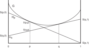
Figure 1: Illustration of a proper scoring rule. If the expert reports $p$, its expected score (relative to its true beliefs) is given by the subtangent hyperplane $H_{p}$. For any report $q$ different from $p$, the expected score $S(q,p)=H_{q}\cdot p$ must be less than the expected score $S(p,p)=H_{p}\cdot p$ of truthful reporting.

There are a number of prediction market mechanisms that allow the principal to extract information from multiple experts; see [16, 5] for excellent surveys. Here we focus on market scoring rules (MSRs) [9, 11], which allow experts to (sequentially) change the forecasted $\mathbf{p}$ using any proper scoring rule $S$. Given the current forecast $\mathbf{p}^{\prime}$, an expert can change the forecast to $\mathbf{p}$ if she is willing to pay according to $S(\mathbf{p}^{\prime},\cdot)$ and receive payment $S(\mathbf{p},\cdot)$. If her true beliefs $\mathbf{p}$ are different from $\mathbf{p}^{\prime}$ and the scoring rule is strictly proper, then she has incentive to participate and report truthfully. Under certain conditions, MSRs can be interpreted as automated market makers [4]. Since each expert pays the amount due to the previous expert for her prediction, the net payment of the principal is the score associated with the final prediction.

3 Scoring Rules for Self-interested Experts

Scoring rules in standard models assume that an expert offering a forecast is uninterested in any aspect her forecast other than the score she will derive from her prediction. As discussed above, there are many settings where the principal will make a decision based on the received forecast, and the expert has a direct interest in this decision. In this section, we develop a model for this situation and devise a class of scoring rules that incentive self-interested agents to report their true beliefs.

3.1 Model Formulation

We assume the principal, or decision maker (DM), will elicit a forecast of $\mathcal{X}$ from expert $E$, and make a decision that is influenced by this forecast. Let $D=\{d_{1},\ldots,d_{n}\}$ be the set of possible decisions, and $u_{ij}$ be DM’s utility should it take decision $d_{i}$ with $x_{j}$ being the realization of $\mathcal{X}$. Letting $\mathbf{u}_{i}=\langle u_{i1},\cdots,u_{im}\rangle$, the expected utility of decision $d_{i}$ given distribution $\mathbf{p}$ is $U_{i}(\mathbf{p})=\mathbf{u}_{i}\cdot\mathbf{p}$. For any beliefs $\mathbf{p}$, DM will want to take the decision that maximizes expected utility, giving DM the utility function $U(\mathbf{p})=\max_{i\leq n}U_{i}(\mathbf{p})$. Since each $U_{i}$ is a linear function of $\mathbf{p}$, $U$ is piecewise linear and convex (PWLC). Furthermore, each $d_{i}$ is optimal in a (possibly empty) convex region of belief space $D_{i}=\{\mathbf{p}:\mathbf{u}_{i}\cdot\mathbf{p}\geq\mathbf{u}_{j}\cdot\mathbf{p},\forall j\}.$ We assume DM acts optimally and that it has a policy $\pi:\Delta(X)\rightarrow D$ that selects some optimal decision $\pi(\mathbf{p})$ for any expert forecast $\mathbf{p}$. In what follows, we take $D_{i}=\pi^{-1}(d_{i})$. We denote by $D_{ij}$ the (possibly empty) boundary between $D_{i}$ and $D_{j}$. Notice that for any $\mathbf{p}\in D_{ij}$ we must have $U_{i}(\mathbf{p})=U_{j}(\mathbf{p})$.

In our running example, suppose the mayor must decide whether to hold a civic ceremony in the town park or at a private banquet facility. Given a forecast probability $p$ of rain, she will make outdoor arrangements at the park if $p$ falls below some threshold $\tau$, and will rent the banquet facility if $p$ is above $\tau$ (here $\tau$ is the indifference probability: $U_{\mbox{\scriptsize park}}(\tau)=U_{\mbox{\scriptsize banq}}(\tau)$).

We note that this model of DM utility is slightly more restricted than that of [13, 3], who allow the utility of each decision to depend on a different random variable, and assume that the realization of a variable will be observed only if the corresponding decision is taken. This introduces difficulties in offering suitable incentives for participation that do not arise in our setting; indeed, the primary contribution of Othman and Sandholm [6], and the extension by Chen and Kash [3], is a characterization of a form of proper scoring in the face of these complications. We also confine our attention primarily to a principal that maximizes its expected utility given $E$’s report (in the terminology of [13], DM uses the max decision rule), though we remark on the possible use of stochastic policies by DM in Sec. 4.2.

Now suppose a single expert $E$ is asked to provide a forecast of $\mathcal{X}$ that permits DM to make a decision. Assume that $E$ knows DM’s policy $\pi$: knowledge of DM’s utility function is sufficient for knowledge of the policy but is not required (we discuss the possibility of $E$ being uncertain about $\pi$ in Sec. 4.1). Further, assume that $E$ has its own utility function or bias $b$, where $b_{ij}$ is $E$’s utility should DM take decision $d_{i}$ and $x_{j}$ is the realization of $\mathcal{X}$. Define $\mathbf{b}_{i}=\langle b_{i1},\cdots,b_{im}\rangle$; and let $E$’s expected utility for $d_{i}$ given $\mathbf{p}$ be $B_{i}(\mathbf{p})=\mathbf{b}_{i}\cdot\mathbf{p}$. In our small example, the weather forecaster may be related to the owner of the banquet facility, and will get some degree of satisfaction (or a small kickback) if the mayor’s ceremony is held there.

As with DM, $E$’s optimal utility function $B^{*}$ (if DM were acting on $E$’s behalf) is PWLC:

$$B^{*}(\mathbf{p})=\max_{i}\mathbf{b}_{i}\cdot\mathbf{p}.$$ (3)

Denote by $D^{*}(\mathbf{p})$ the decision $d_{i}$ that maximizes Eq. 3, i.e., $E$’s preferred decision given beliefs $\mathbf{p}$ (see Fig. 2 for an illustration).

Of course, DM is pursuing its own policy $\pi$, not acting to optimize $E$’s utility. Hence $E$’s actual utility for a specific report $\mathbf{r}$ under beliefs $\mathbf{p}$ is given by

$$B^{\pi}(\mathbf{r},\mathbf{p})=\mathbf{b}_{\pi(\mathbf{r})}\cdot\mathbf{p};$$ (4)

that is, if she reports $\mathbf{r}$, DM will take decision $\pi(\mathbf{r})=d_{k}$ for some $k$, and she will derive benefit $B_{k}(\mathbf{p})$. We refer to $B^{\pi}(\mathbf{r},\mathbf{p})$ as $E$’s inherent utility for reporting $\mathbf{r}$. Similarly, $B(\mathbf{r},x_{i})=b_{i,\pi(\mathbf{r})}$ is $E$’s inherent utility for report $\mathbf{r}$ under realization $x_{i}$. This is simply the inherent benefit she derives from the decision she induces DM to take. This is illustrated in Fig. 2. Notice that $E$’s utility for reports, given any fixed beliefs $\mathbf{p}$, is not generally continuous, with potential (jump) discontinuities at DM’s decision boundaries.

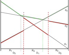
Figure 2: Expert utility function. $E$’s utility for each decision $d_{i}$ is given by the corresponding hyperplane (here, thin black line). $E$’s “optimal” utility $B^{*}$ is the PWLC function shown by the dotted green line (i.e., the upper surface), with each $R_{i}$ denoting the regions of belief space where $D^{*}(\mathbf{p})=d_{i}$. Regions $D_{i}$ represent DM’s policy, where $\pi(\mathbf{p})=d_{i}$ for $\mathbf{p}\in D_{i}$. The thick red lines denote the (discontinuous) utility $B^{\pi}$ that $E$ will receive from (truthfully) reporting her belief.

Without some scoring rule, there is a clear incentive for $E$ to misreport its true beliefs to induce DM to take a decision that $E$ prefers, thereby causing DM to take a suboptimal decision. For instance, in Fig. 2, if $E$’s true beliefs $\mathbf{p}$ lie in $R_{1}$, its preferred decision is $d_{1}$; but truthful reporting will induce DM to take decision $d_{3}$. $E$ has greater inherent utility for reporting (any) $\mathbf{r}\in D_{1}$. Indeed, its gain from the misreport is $\mathbf{p}\cdot(\mathbf{b}_{1}-\mathbf{b}_{3})$. Equivalently, $E$ stands to lose $\mathbf{p}\cdot(\mathbf{b}_{1}-\mathbf{b}_{3})$ by reporting truthfully. Intuitively, a proper scoring rule would remove this incentive to misreport.

3.2 Compensation Rules

If DM knows $E$ utility function, it could reason about $E$’s incentive to misreport and revise its decision policy accordingly. Of course, this would naturally lead to a Bayesian game requiring analysis of its Bayes-Nash equilibria, and generally leaving DM with uncertainty about $E$’s true beliefs. Instead, we wish to derive a scoring rule that DM can use to incentivize $E$ to report truthfully.

A compensation function $C:\Delta(X)\times X\rightarrow\mathbb{R}$ is a mapping from reports and outcomes into payoffs, exactly like a standard scoring rule. Unlike a scoring rule, however, $C$ does not fully determine $E$’s utility for a report; one must also take into account the inherent utility $E$ derives from the decision it prompts the DM to take. Any compensation function $C$ induces a net scoring function:

$$S(\mathbf{p},x_{i}) =C(\mathbf{p},x_{i})+B^{\pi}(\mathbf{p},x_{i})$$ (5)

$E$’s expected net score for report $\mathbf{r}$ under beliefs $\mathbf{p}$ is $S(\mathbf{r},\mathbf{p})=C(\mathbf{r},\mathbf{p})+B^{\pi}(\mathbf{r},\mathbf{p})$, where $C(\mathbf{r},\mathbf{p})=\sum_{i}p_{i}C(\mathbf{r},x_{i})$ is $E$’s expected compensation.

One natural way to structure the compensation function is to use $C$ to compensate $E$ for the loss in inherent utility incurred by reporting its true beliefs $\mathbf{p}$ (relative to its best report). This would remove any incentive for $E$ to misreport. We define a particular compensation function $C_{1}$ that accounts for this loss:

$$C_{1}(\mathbf{p},x_{i})=b_{i,D^{*}(\mathbf{p})}-b_{i,\pi(\mathbf{p})}.$$ (6)

$C_{1}(\mathbf{p},x_{i})$ is simply the difference between $E$’s realized utility for its optimal decision (relative to its report $\mathbf{p}$) and the actual decision she induced. $C_{1}$ does not satisfy the usual properties of scoring rules: it is given by a subgradient of the loss function, which is not convex, nor even continuous. However, $E$’s payoff for a report consists of both this compensation and its inherent utility, i.e., her net score:

$$S_{1}(\mathbf{p},x_{i}) =C_{1}(\mathbf{p},x_{i})+B^{\pi}(\mathbf{p},x_{i})$$ (7)

$$=(b_{i,D^{*}(\mathbf{p})}-b_{i,\pi(\mathbf{p})})+b_{i,\pi(\mathbf{p})})$$ (8)

$$=b_{i,D^{*}(\mathbf{p})}$$ (9)

$E$’s expected net score under beliefs $\mathbf{p}$ is identical to her expected utility for the optimal decision $D^{*}(\mathbf{p})$. Hence, no other report can induce a decision that gives her greater utility. Informally, this shows that truthful reporting is optimal. It can be seen directly by observing that the net score $S_{1}$ can be derived from Eq. 2 by letting $G(\mathbf{p})=B^{*}(\mathbf{p})=\max_{i\leq n}B_{i}(\mathbf{p})$ be $E$’s optimal utility function (which is PWLC, hence convex), and using the subgradient $G^{*}(\mathbf{p})$ given by the hyperplane corresponding to the optimal decision $D^{*}(\mathbf{p})$ at that point.

Definition 2

A compensation function $C$ is proper iff the expected net score function $S$ satisfies $S(\mathbf{p},\mathbf{p})\geq S(\mathbf{q},\mathbf{p})$ for all $\mathbf{p},\mathbf{q}\in\Delta(X)$. $C$ is strictly proper if the inequality is strict.

We don’t prove this formally since we prove a more general result below, but the above informal argument shows:

Proposition 3

Compensation function $C_{1}$ is proper.

Remark 4

We’ve defined the compensation function using the space of all decisions $D$. However, this may cause DM to compensate $E$ for decisions it will never take. If we restrict attention to those decisions in the range of DM’s policy $\pi$, then the above characterization still applies (and will typically reduce total compensation). In what follows, we assume the set of decisions has been pruned to include only those $d\in D$ for which $\pi^{-1}(d)\neq\emptyset$, and that $E$’s utility function is defined relative to that set.

Compensation function $C_{1}$, while proper, is not strictly proper. The induced net scoring function $S_{1}$ is characterized by a non-strictly convex cost function $G$, since $G=B^{*}$. In particular, for any region $R(d)$ of belief space where a single decision $d$ is optimal for $E$, every report $\mathbf{p}\in R(d)$ has the same expected net score, hence there is no “positive” incentive for truthtelling.

While $C_{1}$ gives us one mechanism for proper scoring with self-interested experts, we can generalize the approach to provide a complete characterization of all proper (and strictly proper) compensation functions. We derived $C_{1}$ by compensating $E$ for its loss due to truthful reporting. This approach is more “generous” than necessary. Rather than compensating $E$ for its loss, we need only remove the potential gain from misreporting. The key component of $C_{1}$ is not the “compensation term” $b_{i,D^{*}(\mathbf{p})}$, but rather the the penalty term $-b_{i,\pi(\mathbf{p})}$. It is this penalty that prevents $E$ from benefiting by changing DM’s decision. Any such gain is subtracted from its compensation by the inclusion of $-b_{i,\pi(\mathbf{p})}$. We insist only that the positive compensation term is convex: it need bear no connection to $E$’s actual utility function to incentivize truthfulness. Indeed, we can fully characterize the space of proper and strictly proper compensation functions:

Theorem 5

A compensation rule $C$ is proper for $E$ iff

$$C(\mathbf{p},x_{i})=G(\mathbf{p})-G^{*}(\mathbf{p})\cdot\mathbf{p}+G^{*}_{i}(\mathbf{p})-b_{i,\pi(\mathbf{p})}$$ (10)

for some convex function $G$, and subgradient $G^{*}$ of $G$. $C$ is strictly proper iff $G$ is strictly convex.

Proof 3.6.

Suppose $C$ is given by Eq. 10. $E$’s utility for a report $\mathbf{p}$ given outcome $x_{i}$ is given by its net score:

$$S(\mathbf{p},x_{i}) =C(\mathbf{p},x_{i})+B^{\pi}(\mathbf{p},x_{i})$$

$$=G(\mathbf{p})-G^{*}(\mathbf{p})\cdot\mathbf{p}+G^{*}_{i}(\mathbf{p})-b_{i,\pi(\mathbf{p})}+b_{i,\pi(\mathbf{p})}$$

$$=G(\mathbf{p})-G^{*}(\mathbf{p})\cdot\mathbf{p}+G^{*}_{i}(\mathbf{p})$$

Since $S$ satisfies the conditions of Thm. 1, the standard proof of propriety of $S$ can be used. Similarly, if $G$ is strictly convex, $S$ is strictly proper.

Conversely, suppose $C$ is proper (so that the induced net score satisfies $S(\mathbf{p},\mathbf{p})\geq S(\mathbf{q},\mathbf{p})$). Define $G(\mathbf{p})=S(\mathbf{p},\mathbf{p})$. If $S$ is proper in this sense, it is easy to show that $S(\mathbf{q},\mathbf{p})$ is a convex function of $\mathbf{q}$ (for fixed beliefs $\mathbf{p}$); and since $G(\mathbf{p})=S(\mathbf{p},\mathbf{p})=\max_{\mathbf{q}}S(\mathbf{q},\mathbf{p})$ is the maximum of a set of convex functions (where the last equality holds because $C$ is proper), $G$ is itself convex. Thm. 1 (or more precisely the method used to prove it) ensures that, for some subgradient $G^{*}$ of $G$, we have $S(\mathbf{p},x_{i})=G(\mathbf{p})-G^{*}(\mathbf{p})\cdot\mathbf{p}+G^{*}_{i}(\mathbf{p})$. Hence,

$$C(\mathbf{p},x_{i}) =S(\mathbf{p},x_{i})-B^{\pi}(\mathbf{p},x_{i})$$

$$=G(\mathbf{p})-G^{*}(\mathbf{p})\cdot\mathbf{p}+G^{*}_{i}(\mathbf{p})-b_{i,\pi(\mathbf{p})}$$

so $C$ has the required form. If $C$ is strictly proper, then $G$ must be strictly convex and Thm. 1 can again be applied.

An illustration of a cost function $G(\mathbf{p})$ that gives rise to a proper compensation function is shown in Fig. 3(a).

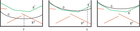
Figure 3: Illustration of the cost functions $G$ that correspond to strictly proper compensation rules. In each figure, $E$’s optimal utility $B^{*}$ is the PWLC function shown in green, and $E$’s inherent utility $B^{\pi}$ is the discontinuous function in red. The net scoring function $G(\mathbf{p})=S(\mathbf{p},\mathbf{p})$, the convex curve, induces an expected compensation function $C(\mathbf{p},\mathbf{p})$ by subtracting $B^{\pi}$. (a) A strictly proper rule that violates weak participation at point $p$. (b) A rule that satisfies weak participation but violates strong participation at point $q$. (c) A rule that satisfies strong participation.

The characterization of Thm. 5 ensures truthful reporting, but may not provide incentives for participation. Indeed, the expert may be forced to pay the DM in expectation for certain beliefs. Specifically, if $G(\mathbf{p})<B^{\pi}(\mathbf{p})$, $E$’s expected compensation $C(\mathbf{p},\mathbf{p})$ is negative. Unless the DM can “force” $E$ to participate, this will cause $E$ to avoid providing a forecast if its beliefs are $\mathbf{p}$ (e.g., see point $p$ is Fig. 3(a)). In general, we’d like to provide $E$ with non-negative expected compensation. We can do this by insisting that the compensation rule weakly incentives participation:

Definition 1.

A compensation function $C$ satisfies weak participation iff for any beliefs $\mathbf{p}$, $E$’s expected compensation for truthful reporting $C(\mathbf{p},\mathbf{p})$ is non-negative.

(See Fig. 3(b) for an illustration of a cost function $G$ that induces a compensation rule $C$ satisfying weak participation.)

Theorem 3.7.

A proper compensation rule $C$ satisfies weak participation iff it meets the conditions of Thm. 5 and $G(\mathbf{p})\geq B^{\pi}(\mathbf{p})$ for all $\mathbf{p}\in\Delta(X)$.

Proof 3.8.

The proof is straightforward: if $G(\mathbf{p})\geq B^{\pi}(\mathbf{p})$ for all $\mathbf{p}$, then for any truthful report $\mathbf{p}$ $E$’s expected compensation is $G(\mathbf{p})-B^{\pi}(\mathbf{p})\geq 0$. Conversely, if $G(\mathbf{p})<B^{\pi}(\mathbf{p})$ for some $\mathbf{p}$, then if $E$ holds beliefs $\mathbf{p}$, a truthful report has negative expected compensation $G(\mathbf{p})-B^{\pi}(\mathbf{p})<0$.

While weak participation seems desirable, even it is not strong enough to ensure an expert’s participation in the mechanism in general. Suppose we define a compensation function using some convex cost function $G(\mathbf{p})$. If $E$ participates, she will maximize her net payoff by reporting her true beliefs, say, $\mathbf{p}$. But suppose that $G(\mathbf{p})<B^{*}(\mathbf{p})$. While $E$ may not be certain how DM will act without its input (e.g., she may not know DM’s “default beliefs” precisely), she may nevertheless have beliefs about DM’s default policy. And, if $E$ believes DM will take decision $D^{*}(\mathbf{p})$ if she provides no forecast, then she will be better off not participating and taking the expected payoff $B^{*}(\mathbf{p})$ derived solely from her inherent utility, and forego participation in the mechanism (which limits her expected payoff to $G(\mathbf{p})$). (See point $q$ in Fig. 3(b).) To prevent this we can require that $C$ strongly incentivize participation, by insisting no matter what $E$ believes about DM’s default policy (i.e., its action given no reporting), it will not sacrifice expected utility by participating in the mechanism.

Definition 2.

A compensation function $C$ satisfies strong participation iff, for any decision $d_{i}\in D$, for any beliefs $\mathbf{p}$, $E$’s net score for truthful reporting is no less than $B_{i}(\mathbf{p})$.

Strong participation means that $E$ has no incentive to abstain from participation (and need not “take its chances” that DM will make a decision it likes). This definition is equivalent to requiring that $E$’s expected utility for truthful reporting, as a function of $\mathbf{p}$ is at least as great as her optimal utility function, i.e., $S(\mathbf{p},\mathbf{p})\geq B^{*}(\mathbf{p})$ for all $\mathbf{p}\in\Delta(X)$. Fig. 3(c) illustrates such a compensation rule.

Theorem 3.9.

Proper compensation rule $C$ satisfies strong participation iff it meets the conditions of Thm. 5 and $G(\mathbf{p})\geq B^{*}(\mathbf{p})$ for all $\mathbf{p}\in\Delta(X)$.

Proof 3.10.

The proof is straightforward. Suppose $G(\mathbf{p})\geq B^{*}(\mathbf{p})$ for all $\mathbf{p}$. If $E$ holds beliefs $\mathbf{p}$, then a truthful report has expected net score of $G(\mathbf{p})\geq B^{*}(\mathbf{p})$, and for no beliefs about DM’s default policy can $E$ derive higher utility by not participating. Conversely, suppose $G(\mathbf{p})<B^{*}(\mathbf{p})$ for some $\mathbf{p}$. If $E$ holds beliefs $\mathbf{p}$ and also believes that DM will take action $d=D^{*}(\mathbf{p})$ if $E$ does not report, then $E$ will derive utility $B^{*}(\mathbf{p})$ by not participating, better than the optimal expected score $G(\mathbf{p})$ from participating.

Observation 3.11

Compensation rule $C_{1}$ is the unique minimal (non-strictly) proper rule satisfying strong participation. That is, no compensation rule offers lower compensation for any report without violating strong participation.

In general, if we insist on strong participation, DM must provide potential compensation up to the level of $E$’s maximum utility gap:

$$g(B)=\max_{i\leq m,j,k\leq n}b_{ik}-b_{ij}.$$

However, this degree of compensation is needed only if DM and $E$ have “directly conflicting” interests (i.e., DM takes a decision whose realized utility is as far from optimal as possible from $E$’s perspective). In such cases, one would expect $E$’s utility to be significantly less than DM’s. If not, this compensation would not be worthwhile for DM. Conversely, if $E$’s interests are well aligned with those of DM, the total compensation required will be small. The most extreme case of well-aligned utility is one where functions $\pi$ and $D^{*}$ coincide, i.e., $\pi(\mathbf{p})=D^{*}(\mathbf{p})$ for all beliefs $\mathbf{p}$, in which case, no compensation is required. Specifically, compensation function $C_{1}(\mathbf{p})=0$ for all $\mathbf{p}$; and while $C_{1}$ is not strictly proper, the only misreports that $E$ will contemplate (i.e., that do not reduce its net score) are those that cannot change DM’s decision (i.e., cannot impact DM’s utility). As a consequence, DM should elicit forecasts from an expert who either (a) has well-aligned interests in the decisions being contemplated; (b) has interest whose magnitude is small (hence requires modest compensation) relative to DM’s own utility; or (c) can be “forced” to make a prediction (possibly at negative net cost).

4 Policy and Utility Uncertainty

We now relax two key assumptions underlying our compensation rule from Section 3.1: that $E$ knows DM’s policy, and that DM knows $E$’s utility function.

4.1 Policy Uncertainty

We first consider the case where DM does not want to disclose its policy to $E$. For example, suppose DM wanted to forego a truthful compensation rule $C$ and simply rely on a proper scoring rule of the usual form that ignores the $E$’s inherent utility. Thm. 5 shows that DM cannot prevent misreporting in general if it ignores $E$’s inherent utility; hence it can suffer a loss in its own utility. However, by refusing to disclose its policy $\pi$, DM could reduce the incentive for $E$ to misreport. Without accurate knowledge of $\pi$, $E$ would be forced to rely on uncertain beliefs about $\pi$ to determine the utility of a misreport, generally lowering its incentive. However, this will not remove the misreporting incentive completely. For instance, referring to Fig. 2, suppose DM does not disclose $\pi$. If $E$ believes with sufficient probability that the decision boundary between $d_{3}$ and $d_{1}$ is located at the point indicated, it will misreport any forecast $\mathbf{p}$ in region $D_{3}$ sufficiently close to that boundary should DM use a scoring rule rather than a compensation rule. As such, refusing to disclose its policy can be used to reduce, but not eliminate, the incentive to misreport if DM does not want to use a proper compensation rule.

Our analysis in the previous section assumed that $E$ used it knowledge of $\pi$ to determine the report that maximizes her net score. However, DM does not need to disclose $\pi$ to make good use of a compensation rule. It can specify a compensation rule implicitly by announcing its net scoring function $S(\mathbf{p},x_{i})$ (or the cost function $G$ and subgradient $G^{*}$) and promising to deduct $B_{d}\cdot\mathbf{p}$ from this score for whatever decision $d$ it ultimately takes. $E$ need not know in advance what decision will be taken to be incentivized to offer a truthful forecast. Nor does $E$ ever need to know what decisions would have been taken had it reported differently. Thus the only information $E$ needs to learn about $\pi$ is the value of $\pi(\mathbf{p})$ at its reported forecast $\mathbf{p}$; and even this need not be revealed until after the decision is taken (and its outcome realized).

4.2 Uncertainty in Expert Utility

We now consider the more interesting issues that arise when DM is uncertain about the parameters $\mathbf{b}$ of $E$’s utility function. If the DM has a distribution over $\mathbf{b}$, one obvious technique is to specify a proper compensation rule using the expectation of $\mathbf{b}$. This may work reasonably well in practice, depending on the nature of the distribution; but it follows immediately from Thm. 5 that this approach will not induce truthful reporting in general.

Rather than analyzing probabilistic beliefs, we instead suppose that DM has constraints on $\mathbf{b}$ that define a bounded feasible region $\mathcal{B}\subseteq\mathbb{R}^{mn}$ in which $E$’s utility parameters must lie. We will confine our analysis to a simple, but natural class of constraints, specifically, upper and lower bounds on each utility parameter; i.e., assume DM has upper and lower bounds ${b_{ij}\!\!\!\uparrow}$ and ${b_{ij}\!\!\!\downarrow}$, respectively, on each $b_{ij}$. This induces a hyper-rectangular feasible region $\mathcal{B}$. If $\mathcal{B}$ is a more general region (e.g., a polytope defined by more general linear constraints), our analysis below can be applied to the tightest “bounding box” of the feasible region. Again by Thm. 5 it is clear that DM cannot define a proper compensation rule in general: without certain knowledge of $E$’s utility, any proposed “deduction” of inherent utility from $E$’s compensation could mistaken, leading to an incentive to misreport. However, this incentive can be bounded.

Under conditions of utility uncertainty, it is natural for DM to restrict its attention to “consistent” compensation rules:

Definition 3.

Let $\mathcal{B}$ be the set of feasible expert utility functions. A compensation rule is consistent with $\mathcal{B}$ iff it has the form, for some (strictly) convex $G$:

$$C(\mathbf{p},x_{i})=G(\mathbf{p})-G^{*}(\mathbf{p})\cdot\mathbf{p}+G^{*}_{i}(\mathbf{p})-\tilde{b}_{i,\pi(\mathbf{p})}$$ (11)

for some $\tilde{\mathbf{b}}\in\mathcal{B}$.

Notice that consistent compensation rules are naturally linear: intuitively, we select a single consistent estimate of each parameter $\tilde{b_{ij}}\in[{b_{ij}\!\!\!\downarrow},{b_{ij}\!\!\!\uparrow}]$, treat $E$ as if this were her true (linear) utility function, and define $C$ using this estimate. Let’s say DM is $\delta$-certain of $E$’s utility iff ${b_{ij}\!\!\!\uparrow}-{b_{ij}\!\!\!\downarrow}\leq\delta$ for all $i,j$. Then we can bound the incentive for $E$ to misreport as follows:

Theorem 4.12.

If DM is $\delta$-certain of $E$’s utility, then $E$’s incentive to misreport under any consistent compensation rule is bounded by $2\delta$. That is, $S(\mathbf{r},\mathbf{p})-S(\mathbf{p},\mathbf{p})\leq 2\delta$.

Proof 4.13.

Let $\mathbf{p}$ be $E$’s actual beliefs and $\mathbf{r}$ some report.

$$S(\mathbf{r},\mathbf{p}) =[G(\mathbf{r})-\tilde{\mathbf{b}}_{\pi(\mathbf{r})}+\mathbf{b}_{\pi(\mathbf{r})}]\cdot\mathbf{p}$$

$$\leq G(\mathbf{r})\cdot\mathbf{p}+\delta$$

$$\leq G(\mathbf{p})\cdot\mathbf{p}+\delta$$

$$\leq[G(\mathbf{p})-\tilde{\mathbf{b}}_{\pi(\mathbf{p})}+\mathbf{b}_{\pi(\mathbf{p})}+\delta]\cdot\mathbf{p}+\delta$$

$$\leq S(\mathbf{p},\mathbf{p})+2\delta$$

Notice that the proof assumes that: (a) the estimated utility $\tilde{\mathbf{b}}_{\pi(\mathbf{r})}$ for the decision induced by $E$’s report $\mathbf{r}$ underestimates her true utility by $\delta$; and (b) the estimated utility $\tilde{\mathbf{b}}_{\pi(\mathbf{p})}$ for the optimal decision overestimates $E$’s true utility by $\delta$. We can limit the misreporting incentive further by using a uniform compensation rule.

Definition 4.

A consistent compensation rule is uniform if each parameter is estimated by $\tilde{b}_{i,\pi(\mathbf{p})}=\lambda{b_{ij}\!\!\!\downarrow}+(1-\lambda){b_{ij}\!\!\!\uparrow}$ for some fixed $\lambda\in[0,1]$.

For example, if DM uses the lower bound (or midpoint, or upper bound, etc.) of each parameter interval uniformly, we call its compensation rule uniform.

Corollary 4.14.

If DM is $\delta$-certain of $E$’s utility, then $E$’s incentive to misreport under any uniform compensation rule is bounded by $\delta$. That is, $S(\mathbf{r},\mathbf{p})-S(\mathbf{p},\mathbf{p})\leq\delta$.

While bounding the incentive to misreport is somewhat useful, it is more important to understand the impact such misreporting can have on DM. Fortunately, this too can be bounded. The (strict) convexity of $G$ means that the greatest incentive to misreport occurs at the decision boundaries of DM’s policy $\pi$ in Thm. 4.12. Since, by definition, DM is indifferent between the adjacent decisions at any decision boundary, misreports in a bounded region around decision boundaries have limited impact on DM’s utility, as we now show. Specifically, we show that the amount by which $E$ will misreport is bounded using the “degree of convexity” of the cost function $G$, which in turn bounds how much loss in utility DM will realize.

Definition 5.

Let $G$ be a convex cost function with subgradient $G^{*}$. We say $G$ is robust relative to $G^{*}$ with factor $m>0$ iff, for all $\mathbf{p},\mathbf{q}\in\Delta(X)$:

$$G(\mathbf{q})\geq G(\mathbf{p})+G^{*}(\mathbf{p})\cdot(\mathbf{q}-\mathbf{p})+m||\mathbf{q}-\mathbf{p}||_{2}$$ (12)

It is not hard to see that $m$-robustness of the pair $G,G^{*}$ imposes a minimum “penalty” on any expert misreport, as a function of its distance from her true beliefs:

Observation 4.15

Let $C$ be a proper compensation rule based on an $m$-robust cost function $G$ and subgradient $G^{*}$. Let $S$ be the induced net scoring function. Then

$$S(\mathbf{p},\mathbf{p})-S(\mathbf{q},\mathbf{p})\geq m||\mathbf{q}-\mathbf{p}||_{2}.$$

Together with Thm. 4.12, this gives a bound on the degree to which an expert will misreport when an uncertain DM uses a consistent compensation rule.

Corollary 4.16.

Let DM be $\delta$-certain of $E$’s utility and use a consistent compensation rule based on an $m$-robust cost function and subgradient. Let $\mathbf{p}$ be $E$’s true beliefs. Then the report $\mathbf{q}$ that maximizes $E$’s net score satisfies $||\mathbf{q}-\mathbf{p}||_{2}\leq\frac{2\delta}{m}$. If the compensation rule is uniform, then $||\mathbf{q}-\mathbf{p}||_{2}\leq\frac{\delta}{m}$.

In other words, $E$’s utility-maximizing report must be within a bounded distance of her true beliefs if DM uses an $m$-robust cost function to define its compensation rule.

The notion of $m$-robustness is a slight variant of the notion of strong convexity [1] in which we use the specific subgradient $G^{*}$ to measure the “degree of convexity.” In the specific case of twice differentiable cost function $G$, we say $G$ is strongly convex with factor $m$ iff $\nabla^{2}G(\mathbf{p})\succeq mI$ for all $\mathbf{p}\in\Delta(X)$; i.e., if the matrix $\nabla^{2}G(\mathbf{p})-mI$ is positive definite [1]. $m$-convexity is a sufficient condition for the robustness we seek.

Corollary 4.17.

Let DM be $\delta$-certain of $E$’s utility and use a consistent compensation rule based on an $m$-convex, twice differentiable cost function $G$. Let $\mathbf{p}$ be $E$’s true beliefs. Then the report $\mathbf{q}$ that maximizes $E$’s net score satisfies $||\mathbf{q}-\mathbf{p}||_{2}\leq\sqrt{\frac{4\delta}{m}}$. If the compensation rule is uniform, then $||\mathbf{q}-\mathbf{p}||_{2}\leq\sqrt{\frac{2\delta}{m}}$.

Proof 4.18.

$G$’s assumed differentiability ensures its gradient $\nabla G$ is the unique subgradient. Since $G$ is $m$-convex, we have

$$G(\mathbf{q})\geq G(\mathbf{p})+\nabla G^{T}(\mathbf{p})(\mathbf{q}-\mathbf{p})+\frac{m}{2}||\mathbf{q}-\mathbf{p}||_{2}^{2}$$

for all $\mathbf{p},\mathbf{q}\in\Delta(X)$ (see [1]). Hence $E$’s loss in compensation is at least $\frac{m}{2}||\mathbf{q}-\mathbf{p}||_{2}^{2}$. Since its gain in inherent utility by misreporting is bounded by $2\delta$ (Thm. 4.12), setting the former to be no greater than $2\delta$ yields the result. Since the gain in inherent utility under a uniform compensation rule is $\delta$, the stronger bound follows by substituting $\delta$ for $2\delta$ in the preceding argument.

Robustness—and strong convexity if we use a differentiable cost function—allow us to globally bound the maximum degree to which $E$ will misreport. This allows us to give a simple, global bound on the loss in DM utility that results from its uncertainty about the expert’s utility function. Recall that DM’s utility function $U_{i}$ for any decision $d_{i}$ is linear, hence has a constant gradient $\nabla U_{i}$. (We abuse notation and simply write $\nabla U_{i}$ for $\nabla U_{i}(\mathbf{p})$.) The function $U_{i}-U_{j}$ is also linear, given by parameter vector $(\mathbf{u}_{i}-\mathbf{u}_{j})$. Let $\mathbf{e}_{k}$ denote the $n$-dimensional unit vector with a 1 in component $k$ and zeros elsewhere.

Theorem 4.19.

Let DM be $\delta$-certain of $E$’s utility and use a consistent compensation rule based on an $m$-robust cost function and subgradient. Assume $E$ reports to maximize her net score. Then DM’s loss in utility relative to a truthful report by $E$ is at most $\max_{k}[\mathbf{e}_{k}^{T}\max_{i,j}\nabla(U_{i}-U_{j})]\sqrt{n}\frac{2\delta}{m}$. If the compensation rule is uniform, then the bound is tightened by a factor of two.

Proof 4.20.

By Cor. 4.16, $E$’s utility maximizing report $\mathbf{q}$ has an $L_{2}$ distance at most $\frac{2\delta}{m}$ from her true beliefs $\mathbf{p}$. By the Cauchy-Schwartz inequality we have $||\mathbf{q}-\mathbf{p}||_{1}\leq\sqrt{n}||\mathbf{q}-\mathbf{p}||_{2}$, hence bounding its max $L_{1}$-deviation at $\sqrt{n}\frac{2\delta}{m}$. Then DM’s loss for any (utility-maximizing) misreport is:

$$\mathbf{u}_{d(\mathbf{p})} \cdot\mathbf{p}-\mathbf{u}_{d(\mathbf{q})}\cdot\mathbf{p}$$

$$=\mathbf{u}_{d(\mathbf{p})}\cdot\mathbf{q}+\nabla U_{d(\mathbf{p})}(\mathbf{p}-\mathbf{q})-\mathbf{u}_{d(\mathbf{q})}\cdot\mathbf{q}-\nabla U_{d(\mathbf{q})}(\mathbf{p}-\mathbf{q})$$

$$\leq\nabla U_{d(\mathbf{p})}(\mathbf{p}-\mathbf{q})-\nabla U_{d(\mathbf{q})}(\mathbf{p}-\mathbf{q})$$

$$\leq\nabla[U_{d(\mathbf{p})}-U_{d(\mathbf{q})}](\mathbf{p}-\mathbf{q})$$

$$\leq\max_{i,j}\nabla(U_{i}-U_{j})(\mathbf{p}-\mathbf{q})$$

$$\leq\max_{k}[\mathbf{e}_{k}^{T}\max_{i,j}\nabla(U_{i}-U_{j})]\sqrt{n}\frac{2\delta}{m}.$$

Here the first inequality holds by virtue of $\mathbf{u}_{d(\mathbf{p})}\cdot\mathbf{q}\leq\mathbf{u}_{d(\mathbf{q})}\cdot\mathbf{q}$ (since $\mathbf{u}_{d(\mathbf{q})}$ is DM’s optimal decision at $\mathbf{q}$).

The same proof can be adapted to strongly convex cost functions.

Corollary 4.21.

Let DM be $\delta$-certain of $E$’s utility and use a linear compensation rule based on an $m$-convex, twice differentiable cost function $G$. Assume $E$ reports to maximize her net score. Then DM’s loss in utility relative to a truthful report by $E$ is at most $\max_{k}[\mathbf{e}_{k}^{T}\max_{i,j}\nabla(U_{i}-U_{j})]\sqrt{n\frac{4\delta}{m}}$. If the compensation rule is uniform, then the bound is tightened by a factor of two.

The results above all rely on the global robustness or global strong convexity of the cost function $G$. Designing a specific cost function (and if not differentiable, choosing its subgradients) can be challenging if we try to ensure uniform $m$-robustness or $m$-convexity across the entire probability space $\Delta(X)$. But recall that $E$ can only impact DM’s utility if its misreport causes DM to change its decision. This means that the cost function need only induce strong penalties for misreporting near decision boundaries. Furthermore, the strength of these penalties should be related to the rate at which DM’s utility is negatively impacted. For example, suppose $\mathbf{p}$ lies on the decision boundary between region $D_{i}$ and $D_{j}$. If $|\nabla(U_{i}-U_{j})|$ is large, then a misreport in the region around $\mathbf{p}$ will cause a greater loss in utility than if $|\nabla(U_{i}-U_{j})|$ is small. This suggests that the cost function should be more strongly convex (or more robust) near decision boundaries whose corresponding decisions differ significantly in utility, and can be less strong when the decisions are “similar.” See Fig. 4 for an illustration of this point.

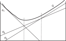
Figure 4: A locally strongly convex cost function $G$. Here $G$ has is more strongly convex in the neighborhood of decision boundary $D_{12}$ than the boundary $D_{23}$. This means an expert willing to sacrifice compensation (e.g., to gain inherent utility due to DM uncertainty) can offer a report that deviates more from its true beliefs in the neighborhood around $D_{23}$ and than it can in the neighborhood around $D_{12}$ for the same loss in compensation. However, since $d_{2}$ and $d_{3}$ are more similar than $d_{1}$ and $d_{2}$ (w.r.t. DM utility), i.e., the gradient $|\nabla(U_{2}-U_{3})|$ is less than $|\nabla(U_{1}-U_{2})|$, DM will lose less utility “per unit” of misreport in the neighborhood of $D_{23}$. Note: the cost function $G$ is drawn above DM’s utility function $U$ for illustration only—in general, it will lie below $U$.

Furthermore, the cost function need only be robust or strongly convex in a local region around these decision boundaries. In particular, suppose $G$ is $m$-robust in some local region around the decision boundary between $D_{i}$ and $D_{j}$. The degree of robustness bounds the maximum deviation from truth that $E$ will contemplate. If the region of $m$-robustness includes these maximal deviations, that will be sufficient to bound DM’s utility loss for any true beliefs $E$ has in that region. Outside of these regions, no misreport by $E$ will cause DM to change its decisions (relative to a truthful report).

We can summarize this as follows:

Definition 6.

$G$ is locally robust relative to $G^{*}$ in the $\varepsilon$-neighborhood around $\mathbf{p}$ with factor $m>0$ iff, for all $\mathbf{q}\in\Delta(X)$ s.t. $||\mathbf{q}-\mathbf{p}||_{2}\leq\varepsilon$:

$$G(\mathbf{q})\geq G(\mathbf{p})+G^{*}(\mathbf{p})\cdot(\mathbf{q}-\mathbf{p})+m||\mathbf{q}-\mathbf{p}||_{2}$$ (13)

Local strong convexity is defined similarly.

Now suppose DM wishes to bound its loss due to misreporting by $E$ by some factor $\sigma>0$. This can be accomplished using a locally robust cost function:

Theorem 4.22.

Let DM be $\delta$-certain of $E$’s utility and fix $\sigma>0$. For any pair of decisions $d_{i},d_{j}$ with non-empty decision boundary $D_{ij}$, define

$$m_{ij}=\!\frac{\max_{k}(\mathbf{e}_{k}^{T}\nabla[U_{i}\!-\!U_{j}])\sqrt{n}2\delta}{\sigma};\;\;\varepsilon_{ij}=\!\frac{\sigma}{\max_{k}(\mathbf{e}_{k}^{T}\nabla[U_{i}\!-\!U_{j}])\sqrt{n}}.$$

Let $G$ be a convex cost function with subgradient $G^{*}$ such that, for all $i,j$ and any $\mathbf{p}\in D_{ij}$, (a) $G$ is locally robust with factor $m_{ij}$ in the $\varepsilon_{ij}$-neighborhood around $\mathbf{p}$; (b) no other decision boundary lies within the $\varepsilon_{ij}$-neighborhood around $\mathbf{p}$. Let DM use a consistent compensation rule based on $G,G^{*}$. Assume $E$ reports to maximize her net score. Then DM’s loss in utility relative to a truthful report by $E$ is at most $\sigma$. If the compensation rule is uniform, the result holds with both $m_{ij}$ and $\varepsilon_{ij}$ decreased by a factor of two.

Proof 4.23.

(Sketch). The proof proceeds by cases involving the location of $E$’s true beliefs $\mathbf{p}$ and the location of possible utility-maximizing misreports $\mathbf{r}$. W.l.o.g., assume that $\mathbf{p}$ is in decision region $D_{i}$. We consider four classes of misreports.

(A) Suppose $\mathbf{r}\in D_{i}$. In this case, DM’s utility loss is zero since the decision is the same as if $E$ had reported truthfully.

(B) Now consider the case where $\mathbf{p}$ is in the $\varepsilon_{ij}$-neighborhood of some decision boundary $D_{ij}$. We show that any report $\mathbf{r}\in D_{j}$ satisfies the condition of the theorem. Let $\mathbf{q}\in D_{j}$ be an arbitrary point s.t. $||\mathbf{q}-\mathbf{p}||_{2}\leq\varepsilon_{ij}$ (this must exist by the assumption that $\mathbf{p}$ lies in the $\varepsilon_{ij}$-neighborhood of $D_{ij}$). DM’s utility loss for reporting $\mathbf{q}$ is then bounded as follows:

$$\mathbf{u}_{i}\cdot\mathbf{p} -\mathbf{u}_{j}\cdot\mathbf{p}$$

$$=\mathbf{u}_{i}\cdot\mathbf{q}+\nabla U_{i}(\mathbf{p}-\mathbf{q})-\mathbf{u}_{j}\cdot\mathbf{q}+\nabla U_{j}(\mathbf{p}-\mathbf{q})$$

$$\leq\nabla[U_{i}-U_{j}](\mathbf{p}-\mathbf{q})$$

$$\leq\max_{k}[\mathbf{e}_{k}^{T}\nabla(U_{i}-U_{j})]||\mathbf{p}-\mathbf{q}||_{1}$$

$$\leq\max_{k}[\mathbf{e}_{k}^{T}\nabla(U_{i}-U_{j})]\sqrt{n}||\mathbf{p}-\mathbf{q}||_{2}$$

$$\leq\max_{k}[\mathbf{e}_{k}^{T}\nabla(U_{i}-U_{j})]\sqrt{n}\varepsilon_{ij}$$

$$=\sigma.$$

If $\mathbf{r}\in D_{j}$, then it must be such a $\mathbf{q}$ (i.e., be within $\varepsilon_{ij}$ of $\mathbf{p}$), since any report in $D_{j}$ has the same inherent utility, while those closest to $\mathbf{p}$ maximize compensation. Hence utility loss for $\mathbf{r}$ is no greater than $\sigma$. Note that $\mathbf{p}$ may lie within the $\varepsilon_{ij}$ neighborhood of multiple decision boundaries $D_{ij}$ adjacent to $D_{i}$, but the argument holds for any report in any such region $D_{j}$.

(C) Now consider the case where boundary $D_{ij}$ exists, but $\mathbf{p}$ does not lie within the $\varepsilon_{ij}$-neighborhood of $D_{ij}$. We show that $E$’s utility maximizing report cannot be in $D_{j}$. By way of contradiction, consider a report $\mathbf{r}\in D_{j}$. Let $\ell$ be the closed line segment $\{(1-\lambda)\mathbf{p}+\lambda\mathbf{r}:\lambda\in[0,1]\}$; and let $\mathbf{q}\in D_{ij}$ be the point where $\ell$ intersects the decision boundary, and let $\mathbf{p}^{\prime}\in D_{i}$ be the point on $\ell$ on the “$D_{i}$ side” of the boundary that is distance $\varepsilon_{ij}$ from the boundary. $E$’s loss in net score (ignoring any error due inherent utility misestimate by DM) is given by:

$$S(\mathbf{p}, \mathbf{p})-S(\mathbf{r},\mathbf{p})$$

$$=H_{\mathbf{p}}\cdot\mathbf{p}-H_{\mathbf{r}}\cdot\mathbf{p}$$

$$=(H_{\mathbf{p}}\!\cdot\!\mathbf{p}-H_{\mathbf{p}^{\prime}}\!\cdot\!\mathbf{p})+(H_{\mathbf{p}^{\prime}}\!\cdot\!\mathbf{p}-H_{\mathbf{q}}\!\cdot\!\mathbf{p})+(H_{\mathbf{q}}\!\cdot\!\mathbf{p}-H_{\mathbf{r}}\!\cdot\!\mathbf{p})$$

We have $(H_{\mathbf{p}}\cdot\mathbf{p}-H_{\mathbf{p}^{\prime}}\cdot\mathbf{p})\geq 0$ by the propriety of the compensation rule (ignoring error due to inherent utility misestimation). We also have

$$H_{\mathbf{p}^{\prime}}\cdot\mathbf{p} -H_{\mathbf{q}}\cdot\mathbf{p}$$

$$=H_{\mathbf{p}^{\prime}}\cdot(\mathbf{p}-\mathbf{p}^{\prime}+\mathbf{p}^{\prime})-H_{\mathbf{q}}\cdot(\mathbf{p}-\mathbf{p}^{\prime}+\mathbf{p}^{\prime})$$

$$=H_{\mathbf{p}^{\prime}}\cdot\mathbf{p}^{\prime}-H_{\mathbf{q}}\cdot\mathbf{p}^{\prime}+H_{\mathbf{p}^{\prime}}\cdot(\mathbf{p}-\mathbf{p}^{\prime})-H_{\mathbf{q}}\cdot(\mathbf{p}-\mathbf{p}^{\prime})$$

$$\geq m_{ij}\varepsilon_{ij}+H_{\mathbf{p}^{\prime}}\cdot(\mathbf{p}-\mathbf{p}^{\prime})-H_{\mathbf{q}}\cdot(\mathbf{p}-\mathbf{p}^{\prime})$$

$$\geq m_{ij}\varepsilon_{ij}$$

$$\geq 2\delta$$

where the first inequality holds due to the local robustness of $G$ and the second due to the convexity of $G$ and the collinearity of $(\mathbf{p},\mathbf{p}^{\prime},\mathbf{q})$. Finally, we must have $(H_{\mathbf{q}}\cdot\mathbf{p}-H_{\mathbf{r}}\cdot\mathbf{p})\geq 0$ again due to the convexity of $G$ and the collinearity of $(\mathbf{p},\mathbf{q},\mathbf{r})$. Thus $E$’s loss in compensation due to misreporting is at least $2\delta$ (and is strictly greater if $G$ is strictly convex). But by Thm. 4.12 its gain in inherent utility by misreporting can be no greater than $2\delta$. Hence its optimal report $\mathbf{r}$ cannot lie in $D_{j}$.

(D) The preceding argument can be adapted in a straightforward way to the case where $D_{i}$ and $D_{j}$ are not adjacent (i.e., $D_{ij}$ is empty).

This result can be generalized to the case where the degree of robustness around one decision boundary is relaxed sufficiently so that the neighborhood within which $E$ can profitably misreport crosses more than one decision boundary (i.e., when another decision boundary overlaps the $\varepsilon_{ij}$-neighborhood around $D_{ij}$). Utility loss will increase but is can be bounded by considering the maximum gradient $\nabla(U_{i}-U_{j})$ over decisions that can be swapped. The result can also be adapted to locally strongly convex cost functions in the obvious way.

Corollary 4.24.

Let DM be $\delta$-certain of $E$’s utility and fix $\sigma>0$. For any pair of decisions $d_{i},d_{j}$ with non-empty decision boundary $D_{ij}$, define

$$m_{ij}=\!\frac{\max_{k}(\mathbf{e}_{k}^{T}\nabla[U_{i}\!-\!U_{j}])\sqrt{n}2\delta}{\sigma};\;\;\varepsilon_{ij}=\!\frac{\sigma}{\max_{k}(\mathbf{e}_{k}^{T}\nabla[U_{i}\!-\!U_{j}])\sqrt{n}}.$$

Let $G$ be a convex cost function such that, for all $i,j$ and any $\mathbf{p}\in D_{ij}$, (a) $G$ is locally convex with factor $m_{ij}$ in the $\varepsilon_{ij}$-neighborhood around $\mathbf{p}$; (b) no other decision boundary lies within the $\varepsilon_{ij}$-neighborhood around $\mathbf{p}$. Let DM use a consistent compensation rule based on $G,G^{*}$. Assume $E$ reports to maximize her net score. Then DM’s loss in utility relative to a truthful report by $E$ is at most $\sigma$.

These results quantify the “cost” to the decision maker of its imprecise knowledge of the expert’s utility function, i.e., its worst-case expected utility relative to what it could have achieved if it had full knowledge of $E$’s utility (i.e., with truthful reporting by $E$).

Remark 4.25.

If we relax the constraint that DM choose the decision $d_{i}$ with maximum expected utility, we can exploit local robustness to induce truthful forecasts. Suppose DM uses the softmax decision policy (see footnote 8): this stochastic policy makes $E$’s utility $B^{\pi}(\mathbf{r},\mathbf{p})$ continuous in its report $\mathbf{r}$. An analysis similar to that above, using local robustness or strong convexity of the cost function, allows DM to induce truthtelling as long as the degree of convexity compensates for the gradient of $B^{\pi}$ at decision boundaries. Since adding randomness to the policy removes the discontinuities in $B^{\pi}$, this is now possible. Of course, this “incentive-compatibility” comes at a cost: the DM is committed to taking suboptimal actions with some probability. We defer a full analysis of the tradeoffs, and the relative benefits of “acting optimally” but risking misleading reports vs. “acting suboptimally” relative to truthful report, to a longer version of this paper.

The characterization of DM loss using local robustness or local strong convexity not only offers theoretical guarantees on DM utility—it has potential operation significance in the design of compensation rules. Specifically, it suggests an optimization procedure for designing a cost function $G$—from which the induced compensation rule $C$ is recovered—so as to minimize DM utility loss. Intuitively, the design of $G$ will attempt to optimize two conflicting objectives: minimizing the bound $\sigma$ on utility loss, which generally requires increasing the degree of robustness or convexity of $G$ at decision boundaries; and minimizing expected compensation $c$ which, given the requirement of strict convexity of $G$, generally requires decreasing robustness or convexity. This tension can be addressed by either: (a) explicitly trading $\sigma$ and $c$ off against each other in the design objective; (b) minimizing $c$ subject to a target bound $\sigma$; or (c) minimizing $\sigma$ subject to a target compensation level $c$. The optimization itself is defined over the space of $n$-dimensional convex curves $G$, and could be treated as an $n$-dimensional spline problem. The objective is to fit a convex function to a set of points with specific local curvature constraints that enforce a certain degree of local convexity at particular decision boundaries. Specific classes of spline functions (e.g., Catmull-Rom splines) might prove useful for this purpose. We leave to future research the question of the practical design of cost and compensation functions under conditions of utility uncertainty.

5 Market Scoring Rules

Space precludes a comprehensive treatment, but we provide a brief sketch of how one might exploit compensation functions in settings where DM aggregates the forecasts of multiple experts. One natural means of doing so is to develop a market scoring rule (MSR) [9, 11] that sequentially applies a standard scoring rule based on how an expert alters the prior forecast (see Sec. 2). The typical means of creating an MSR given a scoring rule $S$ is to have the $k$th expert (implicitly) pay the $k{\!-\!}1$st expert for its forecast according to $S$, and have the principal pay only final expert for its forecast using $S$. In this way, the principal’s total payment is bounded by the maximal possible payment to a single expert [11].

When one attempts this with self-interested experts, difficulties emerge. For instance, Shi et al. [15] show that experts who can alter the outcome distribution after making a forecast, each require compensation to prevent them from manipulating the distribution in ways that are detrimental to the principal. A related form of subsidy arises in our decision setting.

Following [15], we assume a collection of $n$ experts, each of whom can provide alter the forecast $\mathbf{p}$ exactly once. Suppose the experts have an interest in DM’s decision. An “obvious” MSR in our model would simply adopt a proper compensation rule, and have each expert pay the either the compensation or the net score due to the expert who provided the incumbent forecast, and receive her payment from the next expert. If we use compensation, we run into strategic issues. With a proper compensation rule, an expert $k$ reports truthfully based on her net score (total utility), consisting of both compensation and the inherent utility of the decision she induces. In a market setting, $k$’s proposed decision may be changed by the next expert that provides a forecast. This (depending on her beliefs about other expert opinions) may incentivize $k$ to misreport in order to maximize her compensation rather than her net score. Overcoming such strategic issues seems challenging.

Alternatively, each expert might pay the net score due her predecessor. Unfortunately, an arbitrary proper compensation rule may not pay expert $k$ enough score to “cover her costs” (e.g., if $k{\!-\!}1$’s inherent utility is much higher than $k$’s). However, if we set aside issues associated with incentive for participation for the moment, the usual MSR approach can be adapted as follows: we fix a single (strictly) convex cost function $G$ for all experts, and define the compensation rule $C^{k}$ for expert $k$ using $G$ in the usual way:

$$C^{k}(\mathbf{p},x_{i})=G(\mathbf{p})-G^{*}(\mathbf{p})\cdot\mathbf{p}+G^{*}_{i}(\mathbf{p})-b^{k}_{i,\pi(\mathbf{p})},$$

where $\mathbf{b}^{k}$ is $k$’s utility function (bias). If $G$ satisfies strong participation for all experts (i.e., if $G(x_{i})\geq B^{*}(x_{i})$ for all $i$), then any expert $k$ whose beliefs $\mathbf{p}[k]$ differ from the forecast $\mathbf{p}[k{\!-\!}1]$ provided by $k{\!-\!}1$ will have an expected net score (given $\mathbf{p}[k]$) greater than her expected payment to $k{\!-\!}1$ and will maximize her utility by providing a truthful forecast. In particular, let’s denote $k$’s expected payment to $k{\!-\!}1$ by $\rho(k,k{\!-\!}1)$; then we have:

$$\rho(k,k{\!-\!}1) =(H_{\mathbf{p}[k{\!-\!}1]}-\mathbf{b}^{k{\!-\!}1}_{\pi(\mathbf{p}[k{\!-\!}1])})\cdot\mathbf{p}[k]\,+\,\mathbf{b}^{k{\!-\!}1}_{\pi(\mathbf{p}[k{\!-\!}1])}\cdot\mathbf{p}[k]$$

$$=H_{\mathbf{p}[k{\!-\!}1]}\cdot\mathbf{p}[k]$$

$$\leq H_{\mathbf{p}[k]}\cdot\mathbf{p}[k].$$

Hence $k$’s expected payment $\rho(k,k{\!-\!}1)$ is less than its expected net utility, leaving it with a (positive) net gain of $(H_{\mathbf{p}[k]}-H_{\mathbf{p}[k{\!-\!}1]})\cdot\mathbf{p}[k]$. However, this gain may be smaller than the inherent utility she derives from the decision induced by $k{\!-\!}1$, namely, $\mathbf{b}^{k}_{\pi(\mathbf{p}[k{\!-\!}1])}\cdot\mathbf{p}[k]$. Hence this scheme may not incentivize participation. In cases where DM can force participation, such a scheme can be used; but in general, the self-subsidizing nature of standard MSRs cannot be exploited with self-interested experts.

To incentivize participation, DM can subsidize these payments. In the most extreme case, DM simply pays each displaced expert its net utility, which removes any incentives to misreport, but at potentially high cost. In certain circumstances, we can reduce the DM subsidy to the market by having it pay only the inherent utility $b^{k{\!-\!}1}_{i,\pi(\mathbf{p}[k{\!-\!}1])}$ (given realized outcome $x_{i}$) of the displaced expert $k{\!-\!}1$, and requiring the displacing expert $k$ to pay the compensation $H_{i,\mathbf{p}[k{\!-\!}1]}$. Under certain conditions on the relative utility of different experts for different decisions, this is sufficient to induce participation; that is, $k$’s net gain for partipating exceeds her inherent utility for the incumbent decision.

For instance, suppose all experts have the same utility function $\mathbf{b}$ (e.g., consider experts in the same division of a company who are asked to predict the outcome of some event, and have different estimates, but have aligned interests in other respects). In this case, $k$’s net gain for reporting her true beliefs is:

$$(H_{\mathbf{p}[k]} -(H_{\mathbf{p}[k{\!-\!}1]}-\mathbf{b}_{\pi(\mathbf{p}[k{\!-\!}1])}))\cdot\mathbf{p}[k]$$

$$=(H_{\mathbf{p}[k]}-H_{\mathbf{p}[k{\!-\!}1]})\cdot\mathbf{p}[k]+\mathbf{b}_{\pi(\mathbf{p}[k{\!-\!}1])}\cdot\mathbf{p}[k]$$

$$\geq\mathbf{b}_{\pi(\mathbf{p}[k{\!-\!}1])}\cdot\mathbf{p}[k].$$

Hence $k$’s expected net gain is at least as great as her inherent expected utility for the decision induced by $k{\!-\!}1$, and strictly greater if her beliefs differ from those of $k{\!-\!}1$. Thus participation is assured.

Indeed, the argument holds even if the utility functions are not identical: we require only that $k$’s expected utility for the decision it displaces is less than the expected utility (given $k$’s beliefs) to be offered to her predecessor $k{\!-\!}1$. A sufficient condition for this is that $\mathbf{b}^{k}\leq\mathbf{b}^{k{\!-\!}1}$ (pointwise). This suggests that if the DM can elicit predictions of its experts in a particular order, it should do so by eliciting forecasts of those with the greatest utility first.

In general, even in the extreme case of identical expert utility functions, there seems to be no escape from the requirement that DM subsidize the market, at a level that grows linearly with the number of agents. This is very similar to the conclusions drawn by Shi et al. [15]. We provide a more detailed formalization and analysis in an extended version of the paper.

6 Concluding Remarks

We have presented a model that allows the analysis of the incentives facing experts in a decision-making context who have a vested interest in the decision taken by the principal. We have developed a class of compensation rules that are necessary and sufficient to induce truthful forecasts from self-interested experts and also characterized the subclasses of such rules that satisfy weak and strong participation constraints. While vanilla compensation rules assume knowledge of the expert’s utility function on the part of the principal, we’ve also shown how to design compensation rules when the principal has only rough bounds on expert utility parameters in such a way that (a) the incentive for the expert to misreport is bounded; and (b) the impact on the principal’s decision/utility is similarly bounded relative to the case of full knowledge. These bounds are derived from the robustness or strong convexity of the cost function, in either a global or a local sense.

A number of other interesting directions remain. One is the development of computationally effective procedures to design cost functions that minimize principal utility loss in settings where expert utility is not fully known, without inducing extreme degrees of compensation. Another direction is the analysis of the tradeoff between the principal’s decision space and the payments required to induce truthfulness or participation on the part of experts. We discussed above the possibility that by acting (somewhat) suboptimally through the use of a stochastic policy, the principal could diminish the incentive for the expert to misreport. We can take this a step further: intuitively, by limiting its policy to use only a subset of its potential decisions, the principal may dramatically reduce the potential for strategic behavior—either misreporting or failure to participate—on the part of an expert, while at the same time, doing little damage its own utility by restricting its policy in this way.

Finally, the question of joint elicitation both the utility function and the forecast of an expert remains intriguing. This can be viewed as a mechanism design problem where the expert’s type consists of both its preferences and its “information” or forecast (see [6] for a treatment of forecasts themselves from a mechanism design perspective). Preliminary results (joint with Tuomas Sandholm) suggest, not surprisingly, that truthful elicitation is not generally possible when the principal takes a decision that maximizes its expected utility. However, it remains to be seen if effective mechanisms can be designed that offer “reasonable” performance from the perspective of the principal.

Acknowledgements

Thanks to Yiling Chen, Vince Conitzer, Ian Kash, Tuomas Sandholm and Jenn Wortman Vaughan for helpful discussions and suggestions. This work was supported by NSERC.

References

- [1] S. Boyd and L. Vandenberghe. Convex Optimization. Cambridge University Press, Cambridge, 2004.
- [2] G. W. Brier. Verification of forecasts expressed in terms of probability. Monthly Weather Review, 78(1):1–3, 1950.
- [3] Y. Chen and I. Kash. Information elicitation for decision making. In Proceedings of the Tenth International Conference on Autonomous Agents and Multiagent Systems (AAMAS-11), Taipei, 2011. to appear.
- [4] Y. Chen and D. Pennock. A utility framework for bounded-loss market makers. In Proceedings of the Twenty-third Conference on Uncertainty in Artificial Intelligence (UAI-07), pages 49–56, Vancouver, 2007.
- [5] Y. Chen and D. Pennock. Prediction markets. AI Magazine, 31(4):42–52, 2011.
- [6] V. Conitzer. Prediction markets, mechanism design, and cooperative game theory. In Proceedings of the Twenty-fifth Conference on Uncertainty in Artificial Intelligence (UAI-09), pages 101–108, Montreal, 2009.
- [7] S. Dimitrov and R. Sami. Non-myopic strategies in prediction markets. In Proceedings of the Ninth ACM Conference on Electronic Commerce (EC’08), pages 200–209, Chicago, 2008.
- [8] T. Gneiting and A. E. Raftery. Strictly proper scoring rules, prediction, and estimation. Journal of the American Statistical Association, 102(477):359–378, 2007.
- [9] R. Hanson. Combinatorial information market design. Information Systems Frontiers, 5(1):107–119, 2003.
- [10] R. Hanson. Decision markets. IEEE Intelligent Systems, 14(3):16–19, 1997.
- [11] R. Hanson. Logarithmic market scoring rules for modular combinatorial information aggregation. Journal of Prediction Markets, 1(1):3–15, 2007.
- [12] J. McCarthy. Measures of the value of information. Proceedings of the National Academy of Sciences, 42(9):654–655, 1956.
- [13] A. Othman and T. Sandholm. Decision rules and decision markets. In Proceedings of the Ninth International Conference on Autonomous Agents and Multiagent Systems (AAMAS-10), pages 625–632, Toronto, 2010.
- [14] L. J. Savage. Elicitation of personal probabilities and expectations. Journal of the American Statistical Association, 66(336):783–801, 1971.
- [15] P. Shi, V. Conitzer, and M. Guo. Prediction mechanisms that do not incentivize undesirable actions. In Proceedings of the Fifth Workshop on Internet and Network Economics (WINE-09), pages 89–100, Rome, 2009.
- [16] J. Wolfers and E. Zitzewitz. Prediction markets. Journal of Economic Perspectives, 18(2):107–126, 2004.