Resistant estimates for high dimensional and functional data based on random projections
Ricardo Fraiman ∗, and Marcela Svarc ∗∗111Corresponding author: Marcela Svarc, Departamento de Matemáticas y Ciencias, Universidad de San Andrés, Vito Dumas 284, Victoria (1644), Buenos Aires, Argentina. Email: msvarc@udesa.edu.ar
∗Universidad de San Andrés, Argentina and Universidad de la República, Uruguay.
∗∗ Universidad de San Andrés and CONICET, Argentina.
Abstract
We herein propose a new robust estimation method based on random projections that is adaptive and, automatically produces a robust estimate, while enabling easy computations for high or infinite dimensional data. Under some restricted contamination models, the procedure is robust and attains full efficiency. We tested the method using both simulated and real data.
Keywords:
Robust Estimates, Location and Scatter Estimates, Trimming Estimates.
Running Title:
Random Projection Robust Estimates.
1 Introduction
In the problem of robust estimation in high dimensional and functional data, a number of different issues arise that cause the well known robust multivariate estimators to fail, and new ideas are required to address these.
Before stating our proposal, we first review the origins of robustness in order to identify some of the main ideas necessary to guide us in this complex problem.
Ronchetti (2010) who stated that “the primary goal of robust statistics is the development of procedures which are still reliable and reasonably efficient under small deviations from the model, i.e. when the underlying distribution lies in a neighborhood of the assumed model. Robust statistics is then an extension of parametric statistics, taking into account that parametric models are at best only approximations to reality. The field is now some 50 years old. Indeed one can consider Tukey (1960), Huber (1964), and Hampel (1968) the fundamental papers which laid the foundations of modern robust statistics.”
The median. For one dimensional data, the oldest robust estimates are the median and the –trimmed means. The median is in several respects the ‘most robust’ consistent possible location estimate, and great efforts have been made to extend the median and the trimmed means to higher dimensions. The extension of these two simple notions to multivariate data took place via the two main avenues of impartial trimmed means and the concepts of data depth. For the multivariate case Gordaliza (1991) introduced the procedure of impartial trimmed means, which was then extended by Cuesta and Fraiman (2006) for functional data to obtain resistant estimates of the center of a functional distribution. More recently, several proposals considering trimming procedures have been introduced, among them Dolia et al (2007) and Cuevas et al (2008). A number of depth definitions have been introduced for multivariate data, the best known being the Tukey Depth (Tukey, 1975) and the Simplicial Depth (Liu, 1988) and an interesting review of this subject is provided by Serfling (2006). For the case of functional data, several proposals have recently been made, including Fraiman and Muniz (2001), Cuevas and Fraiman (2009), Gervini (2010), among others.
Diagnostic and automatic robust procedures. Two complementary approaches were developed to achieve robustness. Broadly speaking, the different procedures used to flag outliers are known as diagnostic procedures, while the term ‘robustness’ refers to statistical procedures that are insensitive to the effect of outliers. As observed by Serfling (2006), for each depth function one can find a function associated with outlyingness. Hence, several of the foregoing procedures can help in the detection of outliers, such as the proposals of Fraiman and Muniz (2001) and Gervini (2010). Febrero et al (2008) introduced a depth measure for functional data that they used for the identification of outliers.
Many procedures for the identification of outliers have been introduced, among them Rousseeuw and Van Zomeren (1990), Peña and Prieto (2001) and Febrero et al (2007).
In robustness, a class of estimators can be defined in general in terms of the optimization of a specified target functional for the population version of the estimate. Maronna et al (2006), in Chapter 6, presented a detailed review of the different estimates of location and scatter for the multivariate case, describing the properties of each.
In diagnostics, the problem lies in the identification of sub–samples whose deletion maximally changes a statistic of interest as measured by an appropriate target function.
The diagnostic procedure straightforward for one dimensional data, but becomes much more difficult for multivariate data. This is also the case for automatic robust procedures.
Adaptive estimates. In the early 1970’s, some adaptive estimates were proposed for the location model. The word adaptive implied that the estimate adjusted itself in some way to the data concerned. The simplest idea was to consider an M-estimate using Huber’s function, where the parameter (that compromises robustness and efficiency) depends on the data, i.e. (see for instance Yohai, 1974). Roughly speaking, if there are no outliers on the sample, the estimate would tend to choose large values of , while choosing smaller values of correspond to samples that have outliers. These interesting ideas have been neglected ever since.
Neighborhoods. The question arises whether full neighborhoods should be used for some distances between probabilities, or contamination neighborhood should. As mentioned above, we expect robust procedures to be stable under a small deviation from the model, i.e., when the underlying true distribution lies in the neighborhood of the assumed model . Some descriptions of neighborhoods are therefore required. We consider two types, the first being, where is an appropriate distance between probabilities, derived from, for example Prohorov, Kolgomorov or Wasserstein metrics. The second type is of the form where is an arbitrary probability measure. Typically, , which is the case for Prohorov or Kolmogorov (total variation) distances, for example, is particularly appealing, however. It may be perceived that with probability , an observation of the sample comes from a distribution , while for probability it comes from . Recently, Alqallaf et al (2009) considered non standard data contamination models, such as componentwise outliers.
Several notions and measures of robustness have been defined to provide a detailed description of the robustness characteristics of an estimate. The main ideas are:
-
•
Solving minimax problems in a neighborhood of the “true” model. The first approach to formalize the robustness problem was that of Huber‘s (1964, 1981) minimax theory, where the statistical problem is viewed as a game between the Nature (which chooses a distribution in the neighborhood of the model) and the statistician (who chooses a statistical procedure in a given class). The statistician achieves robustness by constructing a minimax procedure that minimizes a lost criterion in which the worst possible distribution in the neighborhood is considered.
-
•
Qualitative robustness. The notion of qualitative robustness was introduced by Hampel (1968) in terms of the equicontinuity of the distribution of the estimate with respect to the Prohorov distance between probabilities.
-
•
Measures of robustness. We herein briefly describe the most important measures of robustness. The influence curve is the infinitesimal approach was introduced by Hampel (1968) within the framework of robust estimation. The finite sample breakdown point (introduced by Donoho and Huber, 1983) of an estimate is the maximum number of observations that can be replaced arbitrarily while the estimate remains bounded (or far away from the boundary of the parameter space when the parameter space is compact). The maximal asymptotic bias as a function of the contamination fraction, measures the worst behavior of an estimate under a fixed proportion of contamination.
Equivariance properties. We expect that any reasonable estimate would only depend on the data, and not on the coordinates axis nor on the scale considered. In the one dimensional problem, the equivariance properties are just the location and the scale equivariance. In the multivariate case, this corresponds to the location equivariance, the orthogonal equivariance, and the global scale equivariance. These properties are still sensible in the infinite dimensional case. However, in the finite dimensional case, the affine equivariance properties often also required. However, this last condition is far from mandatory, and could also be a bad idea. For instance, for contours of multivariate quantiles, the requirement of affine equivariance implies that the contours will be convex sets, losing the important features shown by the non–convex versions that are orthogonal, translation and scale equivariant but not affine equivariant. We consider that the affine equivariance requirement is inadequate for both high and infinite dimensional data. Alqallaf et al (2009) proved that standard high-breakdown affine equivariant estimators propagate outliers under componentwise contamination when the dimension is high. There are many examples of estimates of location and scatter that are not affine equivariant but have many appealing properties (see for instance Maronna and Zamar (2002) or Fraiman and Pateiro-Lopez (2011)).
Computational burden. Most of the robust estimates for multivariate data, particularly those that have improved properties of robustness, are very expensive from a computational point of view and, their computation is unfeasible for high dimensional data. This is also the case with some of the data depth based estimates. In the multivariate case, several attempts have been made in recent years to overcome these problems, by considering resampling algorithms on the initial candidates that allow a substantial reduction in the number of candidates required to obtain a good approximation to the optimal solution (see for instance Van Aelst and Rousseeuw, 2009 or Salibian and Yohai, 2006). In the case of high dimensional or functional data, it is essential that the estimates can be computed in a reasonable time.
Random projections. The idea of using random projections has been already used by several authors in many different contexts. An appealing theoretical framework for the use of random projections can be found in Cuesta, Fraiman and Ransford (2006, 2007).
We herein propose a new robust estimation procedure based on random projections that is data–adaptive, produces automatic robust estimates and combines ideas from the diagnostic framework. In addition it has very low cost when applied to high or infinite dimensional data. The method yields robust estimates that are location and scale equivariant and are also invariant under unitary operators (orthogonal transformations in the finite dimensional case).
The remainder of the paper is organized as follows. In Section 2 we present our general method, and we exemplify with location and scatter estimates. In Section 3 we provide some asymptotic results. Section 4 is devoted to analysis of the performance of the procedure on simulations of the finite dimensional case and also for the case of functional data. In Section 5 we analyze an example using real data. Section 6 includes some final remarks.
2 Our setup
We start by fixing some notation. Let be a real separable Hilbert space, with inner product , and the induced norm . denote a random element in with distribution in a contamination neighborhood of , our “target distribution”.
The data are given by a random sample of iid random elements with the same distribution as .
We are interested in estimating different parameters, including the mean, the covariance operator, and the principal components of a random element with distribution based on the sample . The problem lies in the fact that the distribution of the data is given by rather than .
We assume that is finite and that the covariance operator , is positive definite when is finite dimensional and compact and self-adjoint if is infinite dimensional.
Our aim is to introduce a general method of obtaining consistent robust estimates in this framework that is both suitable for different problems and computationally feasible.
If we were able to select the sub–sample of those random elements that have distribution , from the sample , the problem becomes trivial. We may apply usual “non–robust” estimates to the “good data”.
We propose a trimming scheme based on random projections to select a sub–sample , which we hereafter denote the RT–procedure. The maximum number of observations to be trimmed is . The goal “is to discard only those observations that are far apart from the bulk of the data”. Our method is adaptive in that it stops searching for outliers in a data dependent way.
In the presence of outliers that lie far away from the bulk of the data, there are always several directions (a set of positive probability on the unit sphere with respect to the induced probability measure) where on the projected data, , the outliers are distant from the majority of the observations. If an observation is an outlier this phenomenon is observed in many directions. Therefore, the maximal gap of the one dimensional projected data, will be large, or more precisely, larger than expected. We recall that the maximal gap is the maximum distance between two contiguous observations. On the other hand, those observations that are deep in the bulk of the data set also have deep one dimensional projections in every direction.
However, we may have a shadow cone, where the projected outliers are “hidden” for some directions , as shown on Figure 1.
We seek to define a pruning criterion that combines these two facts. We consider two parameters, the first being , , the maximal trimming rate, the second being, maxiter, the maximal number of random directions that we generate before deciding that all the outliers have been removed.
The subsample selection algorithm.
The following procedure should be repeated either times (where represents the largest integer smaller than or equal to ) or until the number of random directions generated, numdir, reaches maxiter, i.e. while .
-
•
Set .
-
•
Generate a direction at random according to a non-degenerate gaussian measure .
-
•
Project the data on that direction, .
-
•
Sort the projected observations in ascending order .
-
•
Consider the maximum gap .
-
•
If , trim the observation whose one–dimensional projection is most distant from the median of the projected observations, i.e. such that for where .
-
•
Else if , set .
We denote to be the effective trimming rate, i.e., the actual rate of observations that have been reduced.
The value of the threshold on should be related to the limiting behavior of the largest spacing. Deheuvels (1984), characterized it in terms of the local behavior of the density of the observations (in our case the one dimensional projections) in the neighborhood of the point at which it reaches its minimum value. According to Theorem 4, he proved that if the distribution has compact support and the density is bounded away from zero, i.e. there exits such that for every , and if has first derivative then,
This result suggest to take (for sufficiently large values of ) where is a suitable constant greater than 1. There are many univariate distributions that do not have compact support, among which the normal distribution is probably the best known. In practice all the observable data sets have bounded support, hence our consideration of this expression might enable us to determine a useful threshold.
Remark 1. If is a finite dimensional space the random directions can be generated according to an uniform distribution on the unit sphere.
Finally, we compute the ordinary (non–robust estimate) of our target parameters. For instance, the ML mean and covariance estimates are computed only with those observations that have not been trimmed. This implies, that if we assign weight to those observations that have been pruned and to the remainder of the observations, then the mean and the covariance function estimates are given by
respectively, where .
Equivariance properties
The estimates are equivariant under translations, re–scaling and orthogonal transformations. Indeed, it follows from the fact that the weights assigned to the observations are not affected by these operations, because we know that the usual mean and covariance estimates are not affected by them.
It is clear that a shift and re–scaling with a positive constant will not affect the order statistics of the projections, and so the trimmed observations will be the same. Also, if T is an orthogonal transformation, then (because it is an isometry), which means that as the projections do not change, so neither do the weights.
3 Some comments on the asymptotic behavior
Let be iid random elements with the same distribution as defined on , and iid random directions on the unit sphere, independent of and defined on . After performing the algorithm we obtain a subset of random elements , where is random, and each depends on the set of random elements .
The distribution of is , where is the core distribution, is an arbitrary contamination and .
Let be the empirical measure associated with the set of random elements
We wish to identify the conditions under which converges weakly towards , which would imply that for any continuous functional , the estimate defined as will converge to , i.e., we obtain almost sure consistency without assuming any kind of symmetry.
Let be a random element with distribution . As mentioned above we assume that is finite and the covariance operator , is positive definite when is finite dimensional and compact and self-adjoint if is infinite dimensional. Without any loss of generality we also assume that .
We now introduce the following hypotheses:
A1. , for some .
A2.- has a bounded support , and is such that its support verifies that .
This means that the outliers are far from the bulk of the data.
A3.-For all , has a derivable density that fulfils
| (3.1) |
for some , where represents for the support of .
Let be the subset of with , being the corresponding empirical distribution, and .
Because of A1, we may assume that where are iid random elements with distribution , are iid random elements with distribution and are iid random variables with distribution Bernoulli(), being independent the three sets of random elements.
The aim is to show that a.s., where stands for the Prohorov distance when , and at an appropriate rate. This would imply that for any continuous functional , the estimate defined as would converge to . Moreover, we show that in the finite dimensional case, the final estimates will attain “full–efficiency”, meaning that the output of the algorithm will be the set of random elements with distribution . In the infinite dimensional case, an additional assumption will be required in order to attain the “full-efficiency”. Otherwise, under some symmetry conditions on the distribution , regardless of the distribution , the estimate will still be consistent.
A sketch of the proof may be made on the following lines:
First we prove that since , for a sufficiently large we have that a.s.
Since , this is equivalent to show that a.s. for sufficiently large , which follows because by the Hoeffding inequality we have that and .
Second, we show that given with distribution and any with distribution , for in a subset of probability on , there exists and a set of strictly positive probability of directions on for which
| (3.2) |
Indeed, by assumption A2 , we have that for all such that has distribution , with probability . There is therefore a cone of directions where (3.2) holds.
This implies that in the presence of outliers, for sufficiently large values of we can find as many directions as are required for which the maximal spacing of the projected data is be larger than .
Recall that the value of the threshold on is related to the limiting behavior of the largest spacing. Deheuvels (1984) characterized it in terms of the local behavior of the density of the observations (in our case the one dimensional projections) in a neighborhood of the point where it attains its minimum spacing. On Theorem 4, he proves that if the distribution has compact support and the density is bounded away from zero, i.e. there exits such that for every , and if has first derivative then
thus, the maximal spacing behaves like , which converges to zero sufficiently quickly.
Our threshold, which is a constant, is defined as, where is a suitable constant greater than .
Since , the median of the projected data must lie between and .
The foregoing statements and assumption A3 imply that for directions fulfilling (3.2) the maximal spacing will be achieved between some and for with distribution and with distribution or for both with distribution . In both cases an observation with distribution will be deleted. Therefore, for sufficiently large values of , all outliers will be deleted.
The foregoing proofs are insufficient, however. We already know from the previous assertion that for large enough values of the set but we must still prove that the set “behaves as an iid sample of ”, and that . To achieve this goal we need conditions more stringent than (3.1) to hold (see, (3.3) below).
For each fixed direction , let denote the maximal spacing of the set , with cardinal . From assumption A3, and the fact that we have that and thus, for for almost all .
If that holds, then
| (3.3) |
for a sequence , the procedure will end with exactly all observations on the set , and the estimate will attain full efficiency.
In the finite dimensional case, (3.3) is a consequence of assumption A3 (see Proposition 1 below), but this is not the case in the infinite dimensional setting.
Otherwise, we would need to require some symmetry assumptions of the pair . More precisely, we would require that
-
•
has a symmetric distribution around , i.e. and have the same distribution, and that , where is the distribution of a truncation of the random variable , i.e. .
-
•
The density is a decreasing function around for all ,
to obtain consistency. Indeed, it is be a consequence of the symmetry and Theorem 4 in Deheuvels (1984), where it is shown that for any , there exists almost surely a value of such that, for any , the maximal spacing interval is included in .
Proposition 1.
Assume that the support of is a compact connected set with Lebesgue boundary set null, i.e. , and that there exists such that the density of fulfills on . Given a sample of iid random vectors with distribution , let
be the maximal multivariate spacing. We then have that
-
i)
There exists a compact set , , , such that
where is the maximal spacing corresponding to a uniform random sample on .
-
ii)
for all .
-
iii)
where , has the extreme value distribution and and is a known constant. Moreover,
Proof.
The proof of i) is based on a coupling argument. We first demonstrate it for the simple case of . It may be assumed without loss of generality that , and . Let be the uniform distribution on , and iid random variables uniformly distributed on . Let and stand for the cumulative distribution functions, and define , iid samples with distribution and respectively. Since for any pair , , and the derivative of is uniformly greater than that of , we have that which concludes the proof.
The argument for is a little more involved and can be found in Ferrari et al. (2011).
ii) Let be the nearest neighbor of among . For any , , and for any pair we have that . Therefore,
| (3.4) |
and the conclusion follows from (3.4) and i).
iii) These results were obtained by Janson (1987, Theorem1).
∎
4 Simulations
In this Section we discuss the performance of the location, correlation estimates proposed herein, as well as robust principal components estimates. In Subsection 4.1 we analyze the finite dimensional case and the infinite dimensional case is considered in Subsection 4.2. In both cases we compare the RT–estimate with other classical robust estimates and with a benchmark, which is defined below.
4.1 Finite Dimensional Case
We report on the results of a Monte Carlo study, the aim of which was to compare the performance of the Random Trimming (RT) estimates for location and the correlation matrix. It is well known, that the distributions of the original data set and the trimmed data set are different, and if is elliptical the center , coincides with the center of . However, the covariance estimate of and the covariance estimate of have the same shape but differ by a constant . In order to avoid this problem, we estimated the correlation matrix for every case that did not depend on constants. Another approach could have been the computation the minimum and maximum eigenvalues or the matrix condition number. We herein compare our estimates with two different estimates and a benchmark, which we describe below.
a) The Minimum Volume Ellipsoid (MVE) estimate. The MVE estimate was introduced by Rousseeuw (1987); among all the ellipsoids that contain at least half the data points, the one given by the MVE estimate has the minimum volume. Since the computation of this estimate numerically is very expensive unless and are small, a sub–sampling procedure as described by Maronna et al. (2006) is carried out, we denote these estimates (MVEF). We consider these estimates because, despite being very inefficient, they achieve the highest possible breakdown point, if the points are in a general position (this means that no hyperplane contains more than points). In addition, these estimates are the initial estimates usually considered for the computation of S-estimates, and a number of statistical programs, including S-plus, R and SAS, have internal routines to compute them. In these cases the covariance matrix estimation also differs from that of the population by constant, then we compute the correlation matrix.
b) As a benchmark, we compute the mean and correlation classical estimates from the data sets without outliers, and we denote these trick estimates. It is clear that this benchmark attains the best possible behavior.
c) Recently, Gervini (2010) introduced a trimmed estimate for location and scatter, mainly with a view to handling functional data but it was also defined for general Hilbert spaces. Again the idea was to trim the observations that are far away from the bulk of the data set. For each observation he defines the – radius, , , to be the radius of the smallest ball centered on that contains of the observations. In the second stage he trimmed the , , of the observations with higher . We denote these Inter–distances Trimmed Estimates (IT).
Figure 2 shows an example where the performances of the RT and IT estimates are very different. The data are displayed in Figure 2 (a); the grey points correspond to the central distribution and the green ones are the outliers. The contamination rate is . In Figures 2 (b) and (d) the red dots correspond to the observations trimmed by considering the IT procedure where the trimming rates were and respectively. In the first case it was only the outliers that were trimmed, while in the second case some observations from the core distribution were also pruned. In Figures 2 (c) and (d) the pink dots correspond to the observations trimmed by the RT procedure for trimming rates of and respectively. In both cases only the outliers were trimmed.
We consider samples of size on dimensions , and . In all cases a fraction of the observations were taken from a multivariate normal distribution, and the remaining observations are point wise outliers . Because of the equivariance properties of all the estimates considered in this study, the normal observations were taken with a mean of zero and the identity covariance matrix. Moreover, the values of were taken to have the form and took values of and . For the case of the RT-estimate, a direction was considered to be suitable for trimming if the length of the one dimensional gap is bigger than a constant as established on Deheuvels (1984) we took and , which corresponds to , where is the density of a standard normal distribution. The search is carried out in less than random directions. In the case of the IT-estimates we consider , as suggested by Gervini (2010). In both cases the trimming proportions were , and of the data, for the RT–estimates this was the maximum allowable trimming and for the IT–estimates this is the effective pruning rate.
First, we compared the location estimates, and the results are given on Tables 1 and 2. In every case the RT–estimates outperform MVE and MVEF. The behavior of the IT–estimate is remarkable, specially if the outliers are far away from the bulk of the data. If of the observations are outliers and the same amount of data are pruned there are several configurations where the MSE of the trick estimate is achieved. The RT–estimates also perform very well, in that they are better than the IT-estimate if , but not if or . It is important to note that the MSEs for the RT–estimates do not change with the trimming rate, due to the application of a wise trimming strategy.
| Epsilon=0.1 | ||||||||||
|---|---|---|---|---|---|---|---|---|---|---|
| Trick | MVE | MVEF | IT | RT | ||||||
| p | 0.5 | 0.7 | 0.9 | 0.5 | 0.7 | 0.9 | ||||
| 10 | 3 | 0.10 | 0.16 | 0.18 | 0.25 | 0.19 | 0.15 | 0.13 | 0.13 | 0.13 |
| 7 | 0.10 | 0.28 | 0.19 | 0.14 | 0.12 | 0.10 | 0.23 | 0.23 | 0.23 | |
| 11 | 0.10 | 0.36 | 0.15 | 0.14 | 0.12 | 0.10 | 0.14 | 0.14 | 0.15 | |
| 20 | 3 | 0.10 | 0.15 | 0.17 | 0.18 | 0.15 | 0.13 | 0.11 | 0.11 | 0.12 |
| 7 | 0.10 | 0.24 | 0.30 | 0.14 | 0.16 | 0.20 | 0.18 | 0.18 | 0.18 | |
| 11 | 0.10 | 0.35 | 0.42 | 0.14 | 0.12 | 0.10 | 0.26 | 0.26 | 0.26 | |
| 40 | 3 | |||||||||
| 7 | ||||||||||
| 11 | ||||||||||
| Epsilon=0.2 | ||||||||||
|---|---|---|---|---|---|---|---|---|---|---|
| Trick | MVE | MVEF | IT | RT | ||||||
| p | 0.5 | 0.7 | 0.9 | 0.5 | 0.7 | 0.9 | ||||
| 10 | 3 | |||||||||
| 7 | ||||||||||
| 11 | ||||||||||
| 20 | 3 | |||||||||
| 7 | ||||||||||
| 11 | ||||||||||
| 40 | 3 | |||||||||
| 7 | ||||||||||
| 11 | ||||||||||
Tables 3 and 4 show the MSEs for the estimated correlation matrices. In this case the behavior of the RT–estimates is noteworthily, achieving the MSE of the trick estimate, and in almost every circumstance, this method outperforms the others.
| Epsilon=0.1 | ||||||||||
|---|---|---|---|---|---|---|---|---|---|---|
| Trick | MVE | MVEF | IT | RT | ||||||
| p | 0.5 | 0.7 | 0.9 | 0.5 | 0.7 | 0.9 | ||||
| 10 | 3 | |||||||||
| 7 | ||||||||||
| 11 | ||||||||||
| 20 | 3 | |||||||||
| 7 | ||||||||||
| 11 | ||||||||||
| 40 | 3 | |||||||||
| 7 | ||||||||||
| 11 | ||||||||||
| Epsilon=0.2 | ||||||||||
|---|---|---|---|---|---|---|---|---|---|---|
| Trick | MVE | MVEF | IT | RT | ||||||
| p | 0.5 | 0.7 | 0.9 | 0.5 | 0.7 | 0.9 | ||||
| 10 | 3 | |||||||||
| 7 | ||||||||||
| 11 | ||||||||||
| 20 | 3 | |||||||||
| 7 | ||||||||||
| 11 | ||||||||||
| 40 | 3 | |||||||||
| 7 | ||||||||||
| 11 | ||||||||||
Finally, we briefly discuss the computation time. It is well known that MVE is very slow for high dimensional data sets. In our simulations, the MVE is on average between 1300 and 2000 times slower that the trick estimate. The MVEF method takes on average half the time that MVE takes to compute the estimates; nevertheless it is a very slow procedure. Computation times for the IT and RT estimates are very close to the benchmark, particularly for higher dimension. For the two methods are only (respectively ) slower than the trick estimate on average. For dimension they take less than twice the time of the trick estimate to compute the estimations and for dimension they are four times slower. In all cases the RT–estimates are slightly faster than the IT–estimates.
4.2 Functional Data
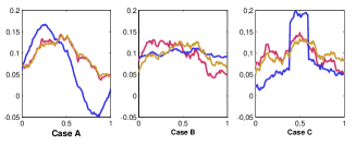
In this Section we study the performance of the RT-estimates of the location and correlation functions for the case of functional data in the presence of outliers. We generate 100 functions, 90 of which follow the central model, , for . and the remaining 10 observations are distributed under one of the following contamination models
Case A. , for The outliers have a different shape from the functions generated by the core distribution.
Case B. , for In these case we consider level shift outliers.
Case C.
In the last case the outliers have the same distribution as the observations generated under the central model, except in the interval where they are shifted as in the previous case. In every case the error of the process follows an Ornstein-Uhlenbeck law, i.e., a Gaussian process with a mean of zero and a covariance function given by,
In Figure 3 we display the three models, the grey functions are generated under the central model while the red ones are the outliers.
For each model we performed 500 replicates where a maximum of either , or of the observations were pruned. Each function was observed at equidistant points on the interval , and the distance between two observations was 0.01. We report the mean number of outliers pruned in table 5. The procedure was very successful at detecting outliers in Cases A and B, however these results changed significantly for Case C where on average more than three outliers are not pruned. Moreover, in Table 6 we show the proportion of observations that are effectively trimmed for each model and trimming proportion and, it can be seen that this proportion does not change as the trimming rate increases.
| Trimmed proportion | |||
|---|---|---|---|
| Case A | |||
| Case B | |||
| Case C | |||
| Trimmed proportion | |||
|---|---|---|---|
| Case A | |||
| Case B | |||
| Case C | |||
In order to analyze the performance of the central and correlation estimates, we consider the –error . Let be the estimate of and be the estimate of , where , then
and
Table 7 exhibits the –error for the location estimates. The first column shows the results for the trick estimate: we consider these results to be the benchmark. From the to the columns the results for the RT–estimates are displayed for three different trimming levels bounds. Finally the results for the IT–estimates proposal with and the same pruning proportion as in our case with hard rejection weights are given on the last three columns. The results for the RT–estimates do not change much for the different estimates. This is because the effective trimming rate and the number of outliers pruned in each replicate are practically the same. IT–estimates show a better performance when the trimming rate is lower, because the contamination proportion is even smaller than the trimming rate. For Models A and B our estimates outperform the IT–estimates, but in Case C the IT–estimates are better because our detection of outliers is less effective. Nevertheless, the performances of the two estimates are very similar and close to the trick estimates. Finally, Table 8 shows the same results for the correlation matrix estimates. The comparison among the estimates shows strong similarities, the main difference being that for Case C our estimates outperform the IT–estimates.
| Trick | RT | IT | |||||
|---|---|---|---|---|---|---|---|
| 0.4 | 0.3 | 0.2 | 0.4 | 0.3 | 0.2 | ||
| Case A | 0.0513 | 0.0637 | 0.0640 | 0.0636 | 0.0725 | 0.0682 | 0.0640 |
| Case B | 0.0513 | 0.0595 | 0.0595 | 0.0596 | 0.0722 | 0.0677 | 0.0630 |
| Case C | 0.0513 | 0.0715 | 0.0714 | 0.0711 | 0.0705 | 0.0670 | 0.0628 |
| Trick | RT | IT | |||||
|---|---|---|---|---|---|---|---|
| 0.4 | 0.3 | 0.2 | 0.4 | 0.3 | 0.2 | ||
| Case A | 0.0779 | 0.1159 | 0.1160 | 0.1153 | 0.1830 | 0.1544 | 0.1262 |
| Case B | 0.0779 | 0.0957 | 0.0953 | 0.0960 | 0.1833 | 0.1543 | 0.1213 |
| Case C | 0.0779 | 0.1213 | 0.1209 | 0.1213 | 0.1814 | 0.1525 | 0.1240 |
The matlab codes for computing the RT-estimate are included as supplemental files.
4.3 Other Classical Statistical Problems
In this Section demonstrate the usefulness of the trimming procedure for other classical statistical problems. The best known dimension reduction technique is that of the principal components, the aim of which is to find a linear combination of the original variables that are uncorrelated and that explain as much of the variability as possible. We consider the same models as in Section 4.2, and trim up to of the data. The results are plotted in Figure 5, in which it can be seen that in every case all the outliers were trimmed. It can be seen that for the cases where the data set is complete (without trimming) the shape of the first principal component weight function is similar to the mean of the contamination. In the three cases, the principal components for the trimmed data sets are similar to the function corresponding to the data set without the outliers.
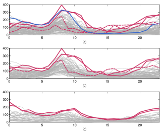
5 A real data example
We now consider the data set of NOx emissions collected in Barcelona, Spain, during the first semester of 2005. The data consists of 127 curves measured 24 times a day, and were first analyzed by Febrero et al. (2007, 2008), in both cases they carried out procedures to detect outliers. There are 12 days for which observations are missing, so they considered the restricted data set conformed by 115 functions. In their first study they found a two cluster structure, corresponding to working days and nonworking days (i.e., Saturdays, Sundays and holidays). They also provided location, scale estimates and set confidence for the NOx data set.
Furthermore, they introduced a distance based procedure to detect outliers. They applied the procedure to the entire set of 115 observations and also to each of the two clusters separately. Febrero et al. (2008) proposed a depth-based criterion for outlier identification, and by using different depth notions on the same data set they proceeded to identify the outliers. In this case they did not analyze the whole data set, but instead they took the subsets of working days and non-working days separately.
The outliers detected by Febrero et al. for the non-working days in both papers are the same (March and April ), while the outliers for the working days do not strictly coincide: in their second paper they detect two outliers (March and April ) while in their first they also detect March to be an outlier.
In this Section we apply our procedure to detect the outliers in the data set and compare the results with those obtained by Febrero et al. (2007, 2008).
When trimming up to of the observations, the results obtained for the working and non-working days coincide with those obtained by Febrero et al. (2007). Figure 6 (b) and (c), shows the observations corresponding to the working and non-working days respectively.
In both cases the solid red observations are the outliers detected by the three procedures and the dashed red line is the new outlier detected only by Febrero el al. (2008).
The analysis of the complete data set can only be compared with the results obtained on Febrero et al. (2007). We detect three outliers, two of which coincide with those found by Febrero el al. (2007) (March and April ), and these observations are shown in Figure 6 (a) as a solid red line, Febrero et al. (2007) classify as outliers two other observations that we do not (March and May), which are plotted as dashed red lines and we find in addition an outlier that they did not, which is indicated as a solid blue line and corresponds to March . The NOx level measured during the dawn and morning of March was very high, however the NOx level during the afternoon is in the bulk of the data. But for March and May the NOx levels during the afternoon are high compared with the others NOx levels measured at the same time, and in general these values are higher than the bulk of the data only for very short periods of time.
6 Concluding Remarks
We have herein presented a new robust estimation method based on random projections that yields robust estimates of location and scatter in general Hilbert spaces. This procedure is data adaptive because it trims only the observations that are far apart from the bulk of the data. It is a particulary suitable procedure for high dimensional data and for functional data because is these estimates are very fast to compute.
References
- [1] Alqallaf, F., Van Aelst, S., Yohai, V. J. and Zamar, R.H. (2009), “Propagation of outliers in multivariate data”. Annals of Statistics, Vol. 37, 311-331.
- [2] Cuesta-Albertos, J.A. and Fraiman, R. (2006). “Impartial means for functional data”. Data Depth: Robust Multivariate Statistical Analysis, Computational Geometry Applications. Eds. R. Liu, R. Serfling and D. Souvaine. American Mathematical Society in DIMACS Series, Vol. 72, 121-145.
- [3] Cuesta-Albertos, J.A., Fraiman, R. and Ransford, T. (2006), “Random projections and goodness-of-fit tests in infinite-dimensional spaces”. Bulletin of the Brazilian Mathematical Society, Vol. 37(4), 1-25.
- [4] Cuesta-Albertos, J.A., Fraiman, R. and Ransford, T.(2007), “A sharp form of the Cramer Wold theorem”. Journal of Theoretical Probability, Vol. 20, 201-209.
- [5] Cuesta-Albertos, J.A., Matran, C. and Mayo-Iscar, A. (2008), “Trimming and likelihood: Robust location and dispersion estimation in the elliptical model”. Annals of Statistics , Vol. 36, 2284-2318.
- [6] Cuevas, A. and Fraiman, R. (2009), “On depth measures and dual statistics. A methodology for dealing with general data”. Journal of Multivariate Analysis, Vol. 100, 753-766.
- [7] Deheuvels, P. (1984), “Limiting Theorems for Maximal Spacings from a General Univariate Distribution”. The Annals of Probability, Vol 12, 1181-1193.
- [8] Dolia, A.N., Harrisb C.J., Shawe-Taylor, J.S. and Titterington, D. M. (2007), “Kernel ellipsoidal trimming”. Computational Statistics and Data Analysis, Vol. 52, 309-324.
- [9] Donoho, D. L. and Huber, P. J. (1983), “The Notion of Breakdown Point”. In Peter J. Bickel, Kjell A. Doksum, and J. L. Hodges, editors, A Festschrift for Erich L. Lehmann, Belmont, CA: Wadsworth.
- [10] Febrero-Bande, M.; Galeano, P. and Gonz lez-Manteiga, W. (2007), “A functional analysis of NOx levels: location and scale estimation and outlier detection”. Computational Statistics,Vol. 22, 411-427.
- [11] Febrero-Bande, M.; Galeano, P. and Gonz lez-Manteiga, W.(2008), “Outlier detection in functional data by depth measures with application to identify abnormal NOx levels”. Envirometrics, Vol. 19, 331-345.
- [12] Ferrari, P., Fraiman, R. and Groisman, P. “About the maximal distance in a point process”, Preprint.
- [13] Fraiman, R. and Muniz, G. (2001), “Trimmed means for functional data”. Test, Vol 10, 419-440.
- [14] Fraiman, R. and Pateiro-Lopez, B. (2011), “Quantiles for functional data”. Preprint.
- [15] Gervini, D. (2010), “Outlier Detection and Trimmed Estimation in General Functional Space”. Preprint. (http://arxiv.org/PS_cache/arxiv/pdf/1001/1001.1014v1.pdf).
- [16] Gordaliza, A. (1991), “Best approximations to random variables based on trimming procedures”. Journal of Approximation Theory, Vol. 64, 162-180
- [17] Hampel F. R. (1968), “Contribution to the Theory of Robust Estimation”. Ph.D Thesis, University of California, Berkeley.
- [18] Hampel F. R. (1974), “The Influence Curve and its Role in Robust Estimation”. Journal of the American Statistical Association, Vol. 69, 383-393.
- [19] Huber, P. J. (1964), “Robust Estimation of a Location Parameter”. Annals of Mathematical Statistics, Vol. 35, 73-101.
- [20] Huber, P. J. (1981), “Robust Statistics”. Wiley.
- [21] Janson, S. (1987), “Maximal Spacing in Several Dimensions”. The Annals of Probability, Vol. 15, 274-280.
- [22] Liu, R. (1988), “On a notion of simplicial depth”. Proceedings of National Academy of Sciences, USA, 85, 1732-1734.
- [23] Maronna, R. A., Martin, R. D. and Yohai, V. J. (2006), “Robust Statistics: Theory and Methods”. Wiley, London.
- [24] Maronna, R. A. and Zamar, R. H. (2002), “Robust Estimation of Location and Dispersion for High Dimensional Data Sets”. Technometric, Vol. 44, 307-317.
- [25] Peña, D. and Prieto, F. (2001), “Multivariate Outlier Detection and Robust Covariance Matrix Estimation”. Technometrics, Vol. 43, 283-310.
- [26] Ronchetti, E. (2010), “Robust Inference”. In: Lovric, Miodrag (Editor), International Encyclopedia of Statistical Science. Heidelberg: Springer Science +Business Media, LLC, reprinted and freely available at StatProb: The Encyclopedia Sponsored by Statistics and Probability Societies.
- [27] Rousseeuw P.J. and Leroy A., (1987), Robust regression and outlier detection. New York, John Wiley.
- [28] Rousseeuw, P.J. and van Zomeren, B.C. (1990), “Unmasking multivariate outliers and leverage points”. Journal of the American Statistical Association, Vol.85, 633-639/648-651.
- [29] Salibian-Barrera, M. and Yohai, V.J. (2006), “A fast algorithm for S-regression estimates”. Journal of Computational and Graphical Statistics, Vol. 15, 414-427.
- [30] Serfling, R. (2006) “Depth Functions in Nonparametric Multivariate Inference”. Data Depth: Robust Multivariate Statistical Analysis, Computational Geometry Applications. Eds. R. Liu, R. Serfling and D. Souvaine. American Mathematical Society in DIMACS Series, Vol. 72, 1-16.
- [31] Tukey, J. W. (1960), “A survey of sampling from contaminated distributions”. In Contributions to Probability and Statistics: Essays in Honor of Harold Hotelling (I. Olkin et al., eds.) 448-485. Stanford Univ. Press.
- [32] Tukey, J. W. (1975), “Mathematics and the picturing of data”. In Proceedings of the International Congress of Mathematicians, Vancouver, 1974 (R. D. James, ed.) 2 523-531. Canadian Mathematical Congress.
- [33] Van Aelst, S. and Rousseeuw, P. (2009), “Minimum volume ellipsoid”. Wiley Interdisciplinary Reviews: Computational Statistics, Vol. 1, 71-82.
- [34] Yohai, V. J. (1974), “ Robust estimation in the linear model”. The Annals of Statistics, Vol. 2, 562-567.