Proton inelastic diffraction by a black nucleus and the size of excited nuclei

Abstract

We systematically derive a length scale characterizing the size of a low-lying, $\beta$ stable nucleus from empirical data for the diffraction peak angle in the proton inelastic differential cross section of incident energy of $\sim 1$ GeV. In doing so, we assume that the target nucleus in the ground state is a completely absorptive “black” sphere of radius $a$. The cross section $\pi a^{2}$, where $a$ is determined in such a way as to reproduce the empirical proton diffraction peak angle in the elastic channel, is known to agree with empirical total reaction cross sections for incident protons to within error bars. By comparing the inelastic diffraction patterns obtained in the Fraunhofer approximation with the experimental ones, one can likewise derive the black sphere radius $a_{l}$ for the excited state with spin $l$. We find that for ¹²C, ^58,60,62,64Ni, and ²⁰⁸Pb, the value of $a_{l}$ obtained from the inelastic channel is generally larger than the value of $a$ from the elastic channel and tends to increase with the excitation energy. This increase is remarkable for the Hoyle state. Finally, we discuss the relation between $a_{l}$ and the size of excited nuclei.

I Introduction

The size of atomic nuclei is one of the most fundamental quantities that characterize matter in the nuclei. It is well known for $\beta$ stable nuclei in the ground state thanks to systematic measurements of electron and proton elastic differential cross sections Bat:ANP . This helps clarify the equation of state of nuclear matter near the saturation point oyaii . For excited states of $\beta$ stable nuclei, however, it is not straightforward to deduce the nuclear size, because elastic scattering off an excited target is hard to measure. Alternatively, one can use proton inelastic differential cross sections in deducing the size of excited nuclei, but all one may know is the transition density, which only implicitly reflects the density distribution of the excited nuclei.

Although one can in principle determine the charge and matter density distributions of a target nucleus from measured electron and proton elastic differential cross sections, it is practically time-consuming even if one uses optical potential models and Glauber’s multiple scattering theory in an approximate manner. Instead of sticking to such microscopic derivations of the nuclear size, in Ref. KIO1 we constructed a phenomenological method for deducing the nuclear size by focusing on the peak angle in the proton-nucleus elastic differential cross section measured at proton incident energy $T_{p}\sim$800-1000 MeV, where the corresponding optical potential is strongly absorptive. In this method, we regard a nucleus as a “black” (i.e., purely absorptive) sphere of radius $a$, and we determine $a$ in such a way that the first peak angle of the Fraunhofer diffraction by a circular black disk of radius $a$ agrees with that of the measured diffraction. This method is reasonable as long as the scattering is close to the limit of the geometrical optics. This condition is fairly well satisfied at least for $T_{p}\gtrsim 800$ MeV, where the wave length of the incident proton is sufficiently shorter than $a$ even for ⁴He. The black sphere picture is originally expected to give a decent description of total reaction cross sections for any kind of incident particle that tends to be attenuated in the nuclear interiors. In fact we showed that for proton beams incident on stable nuclei, the cross section of the black sphere of radius $a$ thus determined is consistent with the measured total reaction cross section KIO2 . If we multiply $a$ by $\sqrt{3/5}$, furthermore, a ratio between the root-mean-square and squared off radii for a rectangular distribution, the result for stable nuclei of $A\gtrsim 50$ shows an excellent agreement with the root-mean-square radius, $r_{m}$, of the matter density distribution as determined from conventional scattering theories so as to reproduce the overall diffraction pattern and analyzing power in the proton elastic scattering KIO1 .

In this paper, we apply the black sphere picture to analyses of proton inelastic scattering data for $T_{p}\sim$1000 MeV. Basically, this application is a straightforward extension of the case of proton elastic scattering, which is closely related to the method developed by Blair Blair for alpha scattering by assuming elastic diffraction by a circular black disk of radius $R_{0}$ and inelastic diffraction by a black nucleus with small multipolar deformations from a sphere of radius $R_{0}$. The present extension is, however, accompanied by a nontrivial choice of the inelastic diffraction peak whose angle is to be fitted to the empirical value and by a variation of the black sphere radius from the value determined from the elastic diffraction peak angle. The resulting black sphere radius does not correspond to the size of the nucleus excited by the incident proton, but rather is related to the transition density and thus expected to lie between the sizes in the ground state and in the excited state. Even so, as we shall see, systematic derivation of the black sphere radius from the inelastic channels is useful for predicting how the size in the excited state depends on the excitation energy $E_{\rm ex}$.

In Sec. II we extend the black sphere approach developed for proton elastic diffraction to the case of proton inelastic diffraction. The results for the black sphere radii are illustrated in Sec. III.

II Black sphere approach

We begin by summarizing the black sphere approach to proton elastic diffraction KIO1 . The center-of-mass (c.m.) scattering angle for proton elastic scattering is generally given by $\theta_{\rm c.m.}=2\sin^{-1}(q/2p)$ with the momentum transfer ${\bf q}$ and the proton incident momentum in the c.m. frame ${\bf p}$. For the proton diffraction by a circular black disk of radius $a$, we can calculate the value of $\theta_{\rm c.m.}$ at the first peak as a function of $a$. (Here we define the zeroth peak as that whose angle corresponds to $\theta_{\rm c.m.}=0$.) We determine $a$ in such a way that this value of $\theta_{\rm c.m.}$ agrees with the first peak angle for the measured diffraction in proton-nucleus elastic scattering, $\theta_{M}$. The radius, $a$, and the angle, $\theta_{M}$, are then related by

$$2pa\sin(\theta_{M}/2)=5.1356\cdots.$$ (1)

By setting

$$r_{\rm BS}\equiv\sqrt{3/5}a,$$ (2)

we found KIO1 that at $T_{p}\gtrsim 800$ MeV, $r_{\rm BS}$, estimated for heavy stable nuclei of $A\gtrsim 50$, is within error bars consistent with the root-mean-square nuclear matter radius, $r_{m}$, deduced from elaborate analyses based on conventional scattering theory. Thus, expression (2) works as a “radius formula.” The factor $\sqrt{3/5}$ comes from the assumption that the nucleon distribution is rectangular; the root-mean-square radius of a rectangular distribution is a cutoff radius multiplied by $\sqrt{3/5}$. For stable nuclei with $A\lesssim 50$, however, the values of $r_{\rm BS}$ are systematically smaller than those of $r_{m}$ KIO2 . The scale $a$ is nevertheless meaningful because the values of $\pi a^{2}$ for C, Sn, and Pb agree well with the proton-nucleus reaction cross section data for $T_{p}\gtrsim 800$ MeV KIO2 . This indicates that $a$ can be regarded as a “reaction radius,” inside which the reaction with incident protons occurs. In a real nucleus, this radius corresponds to the radius at which the mean free path of incident protons is of the order of the length of the penetration. We remark that even for deformed nuclei, this interpretation works well unless the degree of deformations is extremely large.

We now proceed to generalize the black sphere picture to the case of proton inelastic scattering by following a line of argument of Blair Blair . We assume that the final low-lying spin-$l$ excitation of a target even-even nucleus is characterized by small multipolar deformations of a black sphere of radius $a_{l}$. As we will see, this radius generally differs from the value of $a$ obtained from the measured peak angle of elastic diffraction off the same target, as well as among different levels with the same $l$. Therefore, the radius $a_{l}$ is conceptually different from the radius $R_{0}$ used in Ref. Blair . In the adiabatic approximation, which is valid for the proton incident energies, $T_{p}\gtrsim 800$ MeV, of interest here, we may set the reaction radius as

$$R_{l}(\theta,\phi)=a_{l}\left[1+\sum_{m}\alpha_{lm}Y_{lm}(\theta,\phi)\right],$$ (3)

where $\theta$ is measured with respect to the incident beam axis, and $\alpha_{lm}$ are the deformation parameters. For given $\alpha_{lm}$ and ${\bf q}$, we write the scattering amplitude in the c.m. frame of the proton of initial momentum ${\bf p}$ and the black nucleus as

$$f({\bf q};\alpha_{lm}) = \frac{ip}{2\pi}\int_{0}^{2\pi}d\phi\int_{0}^{\infty}dbb$$ (4)

$$\times e^{-i{\bf q}\cdot{\bf b}}\theta(R_{l}(\pi/2,\phi)-b),$$

where ${\bf b}$ is the impact parameter perpendicular to ${\bf p}$. Here we assume that the final proton momentum ${\bf p}+{\bf q}$ has the magnitude equal to that of the initial momentum $p$ because $T_{p}$ is far larger than the excitation energy $E_{\rm ex}$. Then, the c.m. scattering angle again becomes $\theta_{\rm c.m.}=2\sin^{-1}(q/2p)$. With the convention that $\phi$ is measured with respect to the projected final proton momentum onto a plane perpendicular to ${\bf p}$, the scattering amplitude up to linear order in $\alpha_{lm}$ reads

$$f({\bf q};\alpha_{lm}) = \frac{ip}{2\pi}\int_{0}^{2\pi}d\phi\left[\int_{0}^{a_{l}}e^{-iqb\cos\phi}bdb\right.$$ (5)

$$\left.+e^{-iqa_{l}\cos\phi}a_{l}^{2}\sum_{m}\alpha_{lm}Y_{lm}(\pi/2,\phi)\right].$$

The first integral would give the amplitude for elastic scattering off the excited nucleus with spin $l$:

$$\frac{ipa_{l}^{2}J_{1}(2pa_{l}\sin(\theta_{\rm c.m.}/2))}{2pa_{l}\sin(\theta_{\rm c.m.}/2)}.$$ (6)

Note that this amplitude is independent of $\alpha_{lm}$. Anyway, the first integral is beyond the scope of real experiments. The second integral in Eq. (5) leads to the amplitude for inelastic scattering that excites a target nucleus in the ground state to the final state of spin $l$ Blair :

$$ipa_{l}^{2}\sum_{m=-l,-l+2,\cdots}^{l}\left(\frac{2l+1}{4\pi}\right)^{1/2}i^{l}\frac{[(l-m)!(l+m)!]^{1/2}}{(l-m)!!(l+m)!!}$$ (7)

$$\times \alpha_{lm}J_{|m|}(2pa_{l}\sin(\theta_{\rm c.m.}/2)),$$

where $(2n)!!\equiv 2\cdot 4\cdot 6\cdot\cdot\cdot 2n$. The corresponding differential cross section is

$$\frac{d\sigma}{d\Omega}(0\to l) \propto \sum_{m=-l,-l+2,\cdots}^{l}\frac{(l-m)!(l+m)!}{[(l-m)!!(l+m)!!]^{2}}$$ (8)

$$\times\alpha_{lm}^{2}J_{|m|}^{2}(2pa_{l}\sin(\theta_{\rm c.m.}/2)),$$

which gives the inelastic Fraunhofer diffraction pattern.

We next determine $a_{l}$ by comparing the peak angle of the black sphere inelastic diffraction as described by Eq. (8) with the corresponding empirical value $\theta_{Ml}$. Generally, the inelastic diffraction pattern at forward angles is more complicated than the elastic one. We thus avoid the peak that is the nearest to $\theta_{\rm c.m.}=0$ and consider which peak to be chosen among the rest. The guiding principle for this choice is simply to search for the peak that systematically corresponds to the first peak in the elastic diffraction pattern just like the case of electron diffraction Friedrich . We thus obtain

$$2pa_{0}\sin(\theta_{M0}/2)=7.015\cdots,$$ (9)

$$2pa_{2}\sin(\theta_{M2}/2)=6.783\cdots,$$ (10)

$$2pa_{3}\sin(\theta_{M3}/2)=8.209\cdots,$$ (11)

$$2pa_{4}\sin(\theta_{M4}/2)=9.617\cdots.$$ (12)

The values of the right side in Eqs. (9)–(12) correspond to one of the values of $2pa_{l}\sin(\theta_{\rm c.m.}/2)\equiv x$ where Eq. (8) is locally maximal. In fact, the values of $x$ are as follows: For $l=0$, $x=0$, 3.831$\cdots$, 7.015$\cdots$, $\ldots$; for $l=2$, $x=0$, 3.251$\cdots$, 6.783$\cdots$, $\ldots$; for $l=3$, $x=1.982\cdots$, 4.605$\cdots$, 8.209$\cdots$, $\ldots$; for $l=4$, $x=0$, 3.675$\cdots$, 5.852$\cdots$, 9.617$\cdots$, $\ldots$. The choice of other diffraction peaks in extracting $\theta_{Ml}$ would in many cases produce $a_{l}$ that is significantly different from $a$. We remark that the avoidance of the local diffraction maxima at forward angles justifies the neglect of Coulomb effects in the present black sphere approach Blair .

The extraction of $\theta_{Ml}$ from the measured inelastic differential cross sections is not always straightforward for several reasons. Firstly, in the case in which the empirical data lack such diffraction maxima as are supposed to occur in the Fraunhofer diffraction, counting the empirical diffraction maxima does not work. It is thus indispensable to compare the overall measured diffraction pattern with the elastic one whose first peak is easily distinguishable, before identifying the local maxima that give $\theta_{Ml}$. Secondly, even after the local maxima are successfully identified, we need to allow for various uncertainties accompanying determination of $\theta_{Ml}$.

As in the case of elastic scattering KIO1 , we basically determine the values of $\theta_{Ml}$ from the scattering angle that gives the maximum value of the cross section among discrete data near the identified diffraction maximum. Some examples are shown in Fig. 1. When the data stagger in such a way that the scattering angle that gives the local maximum is significantly away from the diffraction peak position deduced from the overall plot of the data, we select the data point that obviously seems the closest to the peak position. Such determination of $\theta_{Ml}$ is accompanied by uncertainties in the measured scattering angle and systematic errors that are dependent on the way of deducing the peak position. The uncertainties in the measured angle, which are due mainly to the absolute angle calibration, are typically of order or smaller than $\pm 0.03$ deg Ray:PRC18 for existing data for proton scattering off stable nuclei. On the other hand, the systematic errors can be estimated by assuming that the true peak is located in the region enclosed by the two data points that are the closest neighbors of the selected data point. The systematic errors thus estimated dominate the error bars of $\theta_{Ml}$, and hence we will ignore the uncertainties in the measured angle.

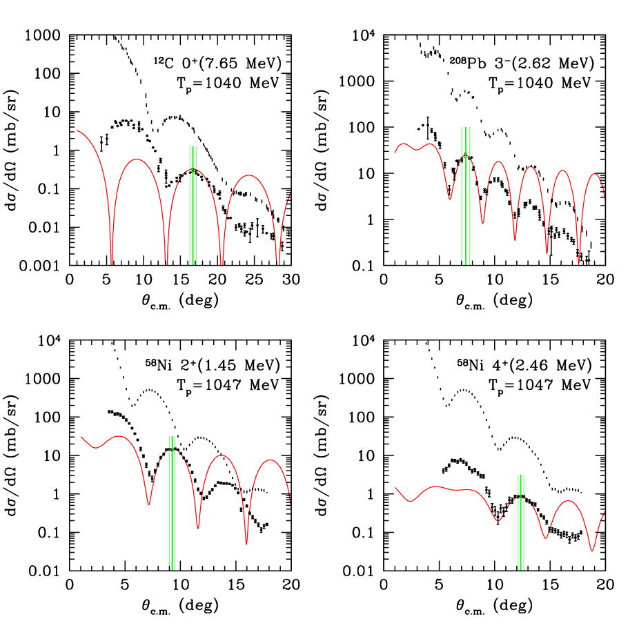
Figure 1: (Color online) The inelastic differential cross section calculated from the Fraunhofer diffraction formula (8) for $p$-¹²C and $p$-²⁰⁸Pb ($T_{p}=1040$ MeV) as well as $p$-⁵⁸Ni ($T_{p}=1047$ MeV). The experimental data (large dots) are taken from Refs. Bertini ; Lombard ; for comparison, the elastic data (small dots) are also plotted. In each panel, the vertical lines denote the peak angle $\theta_{Ml}$ (including error bars) at which we fit the calculated peak angle to the empirical one, and the normalization of Eq. (8) is set in such a way that the value of the differential cross section at $\theta_{Ml}$ agrees with the empirical one.

III Black sphere radii

We finally obtain $a_{l}$ from the determined $\theta_{Ml}$ via Eqs. (9)–(12). For comparison, we likewise determine $\theta_{M}$ and then $a$ via Eq. (1). We remark that a part of the errors of $a_{l}$ and $a$ that come from uncertainties in the proton incident energy, which are typically a few MeV Ray:PRC18 , are negligible. The results for $a$ and $a_{l}$ obtained from empirical scattering data off ¹²C, ^58,60,62,64Ni, and ²⁰⁸Pb at proton incident energy of about 1 GeV Bertini ; Lombard are listed in Table I. In collecting the data, we have made access to the Experimental Nuclear Reaction Data File (EXFOR) IAEA . In the absence of the inelastic scattering data for the $4^{+}$ state of ¹²C and the $2^{+}$ and $4^{+}$ states of ²⁰⁸Pb, the corresponding black sphere radii are unavailable. Note that $a_{3}$ is unavailable for ¹²C despite the presence of the data for the $3^{-}$ state of ¹²C, because the corresponding peak is missing in the measured differential cross section.

Table 1: Black sphere radii obtained from proton elastic and inelastic scattering data.

Target	Final state	$E_{\rm ex}$ (MeV)	$T_{p}$ (MeV)	$a$ or $a_{l}$ (fm)
12C	g.s.	0	1040	2.75$\pm$0.06
	$2^{+}$	4.44	1040	2.70$\pm$0.06
	$0^{+}$	7.65	1040	3.20$\pm$0.07
58Ni	g.s.	0	1047	4.79$\pm$0.18
	$2^{+}$	1.45	1047	4.91$\pm$0.14
	$4^{+}$	2.46	1047	5.22$\pm$0.11
	$3^{-}$	4.47	1047	5.09$\pm$0.13
60Ni	g.s.	0	1047	4.78$\pm$0.18
	$2^{+}$	1.33	1047	4.91$\pm$0.14
	$4^{+}$	2.50	1047	5.22$\pm$0.12
	$3^{-}$	4.04	1047	5.09$\pm$0.13
62Ni	g.s.	0	1047	4.96$\pm$0.19
	$2^{+}$	1.17	1047	5.05$\pm$0.15
	$4^{+}$	2.34	1047	5.22$\pm$0.12
	$3^{-}$	3.76	1047	5.22$\pm$0.13
64Ni	g.s.	0	1047	4.96$\pm$0.19
	$2^{+}$	1.35	1047	5.04$\pm$0.15
	$4^{+}$	2.61	1047	5.22$\pm$0.11
	$3^{-}$	3.55	1047	5.09$\pm$0.13
208Pb	g.s.	0	1040	7.49$\pm$0.35
	$3^{-}$	2.62	1040	7.29$\pm$0.35

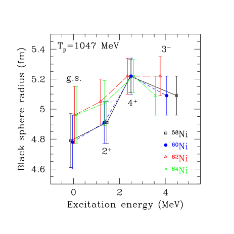
Figure 2: (Color online) The black sphere radius as a function of the excitation energy. The target nucleus is ¹²C, ^58,60,62,64Ni, and ²⁰⁸Pb. For Ni isotopes, the squares (with line), circles (with short-dashed line), triangles (with long-dashed line), and crosses (with dash-dotted line) denote the results for ⁵⁸Ni, ⁶⁰Ni, ⁶²Ni, and ⁶⁴Ni, respectively.

To see the systematic behavior of the black sphere radii, we plot the radii as function of $E_{\rm ex}$ in Fig. 2. We find that the black sphere radius tends to increase with $E_{\rm ex}$, with a few exceptions in which case the black sphere radius decreases with $E_{\rm ex}$ in its central value but can be regarded as unchanged allowing for the error bars. This is consistent with the behavior of the transition radii obtained systematically from electron inelastic scattering off ²⁰⁸Pb Friedrich .

Recall that the black sphere radius $a_{l}$ is related to the transition density and thus expected to lie between the sizes in the ground state and in the excited state. It is thus reasonable that the differences between $a$ and $a_{l}$ for the low-lying excited states of interest here are generally small. The only exception that we discovered is the ¹²C $0^{+}$ state (the Hoyle state), for which $a_{0}/a\simeq 1.16$. The nucleus in the Hoyle state is thus expected to be larger than that in the ground state by more than 16 %, a feature consistent with the $\alpha$-clustering picture of the Hoyle state Takashina .

In summary, we generalized the black-sphere method for deducing the size of the ground-state nuclei from proton-nucleus elastic scattering data to the case of proton-nucleus inelastic scattering data and provided implications for the size of excited nuclei. In the present analysis, we confined ourselves to even-even nuclei. Extension to odd nuclei would be straightforward if the conventional collective model works Blair . It is also important to note that the validity of the inelastic Fraunhofer diffraction formula used here tends to decrease with increasing scattering angle. We assume that the peak selected for determination of $a_{l}$, as shown in Fig. 1, is in the valid regime, which could be checked by microscopically clarifying a relation between the transition density and $a_{l}$ Hashimoto . We hope that the present analysis could develop into a systematic drawing of the black-sphere radii of isomers and nuclei in other characteristic excited states over a chart of the nuclides.

- (1) C.J. Batty, E. Friedman, H.J. Gils, and H. Rebel, Adv. Nucl. Phys. 19, 1 (1989).
- (2) K. Oyamatsu and K. Iida, Prog. Theor. Phys. 109, 631 (2003).
- (3) A. Kohama, K. Iida, and K. Oyamatsu, Phys. Rev. C 69, 064316 (2004).
- (4) A. Kohama, K. Iida, and K. Oyamatsu, Phys. Rev. C 72, 024602 (2005).
- (5) J.S. Blair, Phys. Rev. 115, 928 (1959).
- (6) J. Friedrich, N. Voegler, and H. Euteneuer, Phys. Lett. 64B, 269 (1976).
- (7) L. Ray, W. Rory Coker, and G.W. Hoffmann, Phys. Rev. C 18, 2641 (1978).
- (8) R. Bertini et al., Phys. Lett. 45B, 119 (1973).
- (9) R.M. Lombard, G.D. Alkhazov, and O.A. Domchenkov, Nucl. Phys. A360, 233 (1981).
- (10) The data have been retrieved from EXFOR at IAEA-NDS (International Atomic Energy Agency (IAEA)-Nuclear Data Service (NDS)) web site http://www-nds.iaea.org/
- (11) M. Takashina, Phys. Rev. C 78, 014602 (2008).
- (12) S. Hashimoto, M. Yahiro, K. Ogata, K. Minomo, and S. Chiba, arXiv:1104.1567.