A Semidefinite Programming approach for minimizing ordered weighted averages of rational functions

Abstract.

This paper considers the problem of minimizing the ordered weighted average (or ordered median) function of finitely many rational functions over compact semi-algebraic sets. Ordered weighted averages of rational functions are not, in general, neither rational functions nor the supremum of rational functions so that current results available for the minimization of rational functions cannot be applied to handle these problems. We prove that the problem can be transformed into a new problem embedded in a higher dimension space where it admits a convenient representation. This reformulation admits a hierarchy of SDP relaxations that approximates, up to any degree of accuracy, the optimal value of those problems. We apply this general framework to a broad family of continuous location problems showing that some difficult problems (convex and non-convex) that up to date could only be solved on the plane and with Euclidean distance, can be reasonably solved with different $\ell_{p}$-norms and in any finite dimension space. We illustrate this methodology with some extensive computational results on location problems in the plane and the $3$-dimension space.

1. Introduction

Weighted Averaging (OWA) or Ordered Median Function (OMF) operators provide a parameterized class of mean type aggregation operators (see [25, 44] and the references therein for further details). Many notable mean operators such as the max, arithmetic average, median, k-centrum, range and min, are members of this class. They have been widely used in location theory and computational intelligence because of their ability to represent flexible models of modern logistics and linguistically expressed aggregation instructions in artificial intelligence ([25] and [39, 40, 41, 42, 43, 44]). Weighted averages (or ordered median) of rational functions are not, in general, neither rational functions nor the supremum of rational functions so that current results available for the minimization of rational functions are not applicable. In spite of its intrinsic interest, as far as we know, a common approach for solving this family of problems is not available. Nevertheless, one can find in the literature different methods for solving particular instances of problems within this family, see e.g. [5, 6, 14, 25, 26, 27, 28, 29, 30, 31, 32, 34]. The first goal of this paper is to develop a unified tool for solving this class of optimization problems. In this line, we prove that the general problem can be transformed into a new problem embedded in a higher dimension space where it admits a convenient representation that allows to arbitrarily approximate or to solve it as a minimization problem over an adequate closed semi-algebraic set. Hence, our approach goes beyond a trivial adaptation of current theory.

Regarding the applications, it is commonly agreed that ordered median location problems are among the most important applications of OWA operators. Continuous location has achieved an important degree of maturity. Witnesses of it are the large number of papers and research books published within this field. In addition, this development has been also recognized by the mathematical community since the AMS code 90B85 is reserved for this area of research. Continuous location problems appear very often in economic models of distribution or logistics, in statistics when one tries to find an estimator from a data set or in pure optimization problems where one looks for the optimizer of a certain function. For a comprehensive overview the reader is referred to [4] or [25]. Despite the fact that many continuous location problems rely heavily on a common framework, specific solution approaches have been developed for each of the typical objective functions in location theory (see for instance [4]). To overcome this inflexibility and to work towards a unified approach to location theory the so called Ordered Median Problem (OMP) was developed (see [25] and references therein). Ordered median problems represent as special cases nearly all classical objective functions in location theory, including the Median, CentDian, center and k-centra. More precisely, the 1-facility ordered median problem in the plane can be formulated as follows: A vector of weights $(\lambda_{1},\ldots,\lambda_{n})$ is given. The problem is to find a location for a facility that minimizes the weighted sum of distances where the distance to the closest point to the facility is multiplied by the weight $\lambda_{n}$, the distance to the second closest, by $\lambda_{n-1}$, and so on. The distance to the farthest point is multiplied by $\lambda_{1}$. Many location problems can be formulated as the ordered 1-median problem by selecting appropriate weights. For example, the vector for which all $\lambda_{i}=1$ is the unweighted 1-median problem, the problem where $\lambda_{n}=1$ and all others are equal to zero is the 1-center problem, the problem where $\lambda_{1}=\ldots=\lambda_{k}=1$ and all others are equal to zero is the $k$-centrum. Minimizing the range of distances is achieved by $\lambda_{1}=1$, $\lambda_{n}=-1$ and all others are zero. Despite its full generality, the main drawback of this framework is the difficulty of solving the problems with a unified tool. There have been some successful approaches that are now available whenever the framework space is either discrete (see [2, 22, 30]) or a network (see [11], [12] or [24]). Nevertheless, the continuous case has been, so far, only partially covered. There have been some attempts to overcome this drawback and there are nowadays some available methodologies to tackle these problems, at least in the plane and with Euclidean norm. In Drezner [3] and Drezner and Nickel [5, 6] the authors present two different approaches. The first one uses a continuous branch and bound method based on triangulations (BTST) and the second one on a D-C decomposition for the objective function that allow solving the problems on the plane. More recently, Rodriguez-Chia et al. [34] also address the particular case of the $k$-centrum problem and using geometric arguments develop a better algorithm applicable only for that problem on the plane and Euclidean distances.

Quoting the conclusions of the authors of [5]: “All our experiments were conducted for Euclidean distances. As future research we suggest to test these algorithms on problems (even the same problems) based on other distance measures. (…) Solving k-dimensional problems by a similar approach requires the construction of k-dimensional Voronoi diagrams which is extremely complicated.”

Therefore, the challenge is to design a common approach also to solve the above mentioned family of location problems, for different distances and in any finite dimension. This is essentially the second goal of this paper. In our way, we have addressed the more general problem that consists of the minimization of the OWA operator of a finite number of rational functions over closed semialgebraic sets that is the first goal of this paper. Thus, our second goal is to solve a general class of continuous location problems using the general approach mentioned above for the minimization of OWA rational functions and to show the powerfulness of this methodology. Of course, we know that the problem in its full generality is $NP-hard$ since it includes general instances of convex minimization. Therefore, we cannot expect to obtain polynomial algorithms for this class of problems. Rather, we will apply a new methodology first proposed by Lasserre [16], that provides a hierarchy of semidefinite problems that converge to the optimal solution of the original problem, with the property that each auxiliary problem in the process can be solved in polynomial time.

The paper is organized in 5 sections. The first one is our introduction. In the second section and for the sake of completeness, we recall some general results on the Theory of Moments and Semidefinite Programming (SDP) that will be useful in the rest of the paper. Section 3 considers what we call the $\mathbf{MOMRF}$ problem which consists of minimizing the ordered median function of finitely many rational functions over a compact basic semi-algebraic set. In the spirit of the moment approach developed in Lasserre [16, 18] for polynomial optimization and later adapted by Jibetean and De Klerk [10], we define a hierarchy of semidefinite relaxations (in short SDP relaxations). Each SDP relaxation is a semidefinite program which, up to arbitrary (but fixed) precision, can be solved in polynomial time and the monotone sequence of optimal values associated with the hierarchy converges to the optimal value of $\mathbf{MOMRF}$. Sometimes the convergence is finite and a sufficient condition permits to detect whether a certain relaxation in the hierarchy is exact (i.e. provides the optimal value), and to extract optimal solutions (theoretical bounds on the relaxation order for the exact results can be found in [35, 36]). Section 4 considers a general family of location problems that is built from the problem $\mathbf{MOMRF}$ but which does not actually fits under the same formulation because the objective functions are not quotients of polynomials. Nevertheless, we prove that under a certain reformulation one can define another hierarchy of SDP that fulfils convergence properties ‘$\grave{\mbox{a}}$ la Lasserre’. This approach is applicable to location problems with any $\ell_{p}$-norm ($p\in\mathbb{Q}$) and in any finite dimension space. We exploit the special structure of these problems to find a block diagonal reformulation that reduces the sizes of the SDP relaxations and allows to solve larger instances. Our computational tests are presented in Section 5. We analyze five families of problems, namely, Weber, center, $k$-centrum, trimmed-mean and range. There we show that convergence is rather fast and very high accuracy is achieved in all cases, even with the first feasible relaxation. (We observe that for location problems with Euclidean distances that relaxation order is $r=2$.) The paper ends with some conclusions and an outlook for further research.

2. Preliminaries

In this section we recall the main definitions and results on the moment problem and semidefinite programming that will be useful for the development through this paper. We use standard notation in the field (see e.g. [20]).

We denote by $\mathbb{R}[x]$ the ring of real polynomials in the variables $x=(x_{1},\ldots,x_{n})$, and by $\mathbb{R}[x]_{d}\subset\mathbb{R}[x]$ the space of polynomials of degree at most $d\in\mathbb{N}$ (here $\mathbb{N}$ denotes the set of nonnegative integers). We also denote by $\mathcal{B}=\{x^{\alpha}:\alpha\in\mathbb{N}^{n}\}$ a canonical basis of monomials for $\mathbb{R}[x]$, where $x^{\alpha}=x_{1}^{\alpha_{1}}\cdots x_{n}^{\alpha_{n}}$, for any $\alpha\in\mathbb{N}^{n}$.

For any sequence indexed in the canonical monomial basis $\mathcal{B}$, $\mathbf{y}=(y_{\alpha})_{\alpha\in\mathbb{N}^{n}}\subset\mathbb{R}$, let $\mathrm{L}_{\mathbf{y}}:\mathbb{R}[x]\to\mathbb{R}$ be the linear functional defined, for any $f=\sum_{\alpha\in\mathbb{N}^{n}}f_{\alpha}\,x^{\alpha}\in\mathbb{R}[x]$, as $\mathrm{L}_{\mathbf{y}}(f):=\sum_{\alpha\in\mathbb{N}^{n}}f_{\alpha}\,y_{\alpha}$.

The moment matrix $\mathrm{M}_{d}(\mathbf{y})$ of order $d$ associated with $\mathbf{y}$, has its rows and columns indexed by $(x^{\alpha})$ and $\mathrm{M}_{d}(\mathbf{y})(\alpha,\beta)\,:=\,\mathrm{L}_{\mathbf{y}}(x^{\alpha+\beta})\,=\,y_{\alpha+\beta}$, for $|\alpha|,\,|\beta|\,\leq d.$ Note that the moment matrix is ${{n+d}\choose{n}}\times{{n+d}\choose{n}}$ and that there are ${{n+2d}\choose{n}}$ $\mathbf{y}_{\alpha}$ variables.

For $g\in\mathbb{R}[x]\,(=\sum_{\gamma}g_{\gamma\in\mathbb{N}^{n}}x^{\gamma}$), the localizing matrix $\mathrm{M}_{d}(g,\mathbf{y})$ of order $d$ associated with $\mathbf{y}$ and $g$, has its rows and columns indexed by $(x^{\alpha})$ and $\mathrm{M}_{d}(g,\mathbf{y})(\alpha,\beta):=\mathrm{L}_{\mathbf{y}}(x^{\alpha+\beta}g(x))=\sum_{\gamma}g_{\gamma}y_{\gamma+\alpha+\beta}$, for $|\alpha|,|\beta|\,\leq d$.

Definition 1.

Let $\mathbf{y}=(y_{\alpha})\subset\mathbb{R}$ be a sequence indexed in the canonical monomial basis $\mathcal{B}$. We say that $\mathbf{y}$ has a representing measure supported on a set $\mathbf{K}\subseteq\mathbb{R}^{n}$ if there is some finite Borel measure $\mu$ on $\mathbf{K}$ such that

$$y_{\alpha}\,=\,\int_{\mathbf{K}}x^{\alpha}\,d\mu(x),\mbox{ for all }\alpha\in\mathbb{R}^{n}.$$

The main assumption that is needed to impose when one wants to assure the convergence of the SDP relaxations for solving polynomial optimization problems (see for instance [19, 20]) was introduced by Putinar [33] and it is stated as follows.

Putinar’s Property.

Let $\{g_{1},\ldots,g_{l}\}\subset\mathbb{R}[x]$ and $\mathbf{K}:=\{x\in\mathbb{R}^{d}:g_{j}(x)\geq 0,:j=1,\ldots,\ell\}$ a basic closed semialgebraic set. Then, $\mathbf{K}$ satisfies Putinar’s property if there exists $u\in\mathbb{R}[x]$ such that:

1. $\{x:u(x)\geq 0\}\subset\mathbb{R}^{n}$ is compact, and

2. $u\,=\,\sigma_{0}+\sum_{j=1}^{\ell}\sigma_{j}\,g_{j}$, for some $\sigma_{1},\ldots,\sigma_{l}\in\Sigma[x]$. (This expression is usually called a Putinar’s representation of $u$ over $\mathbf{K}$).

Being $\Sigma[x]\subset\mathbb{R}[x]$ the subset of polynomials that are sums of squares.

Note that Putinar’s property is equivalent to impose that the quadratic polynomial $M-\sum_{i=1}^{n}x_{i}^{2}$ has a Putinar’s representation over $\mathbf{K}$.

We observe that Putinar’s property implies compactness of $\mathbf{K}$. It is easy to see that Putinar’s property holds if either $\{x:g_{j}(x)\geq 0\}$ is compact for some $j$, or all $g_{j}$ are affine and $\mathbf{K}$ is compact. Furthermore, Putinar’s property is not restrictive at all, since any semialgebraic set $\mathbf{K}$ for which is known that $\sum_{i=1}^{n}x_{i}^{2}\leq M$ holds for some $M>0$ and for all $x\in\mathbf{K}$, $\mathbf{K}=\mathbf{K}\cup\{g_{l+1}(x):=M-\sum_{i=1}^{n}x_{i}^{2}\geq 0\}$ verifies Putinar’s property.

The importance of Putinar’s property stems from the following result:

Theorem 2 (Putinar [33]).

Let $\{g_{1},\ldots,g_{l}\}\subset\mathbb{R}[x]$ and $\mathbf{K}:=\{x\in\mathbb{R}^{d}:g_{j}(x)\geq 0,:j=1,\ldots,\ell\}$ satisfying Putinar’s property. Then:

1. Any $f\in\mathbb{R}[x]$ which is strictly positive on $\mathbf{K}$ has a Putinar’s representation over $\mathbf{K}$.

2. $\mathbf{y}=(y_{\alpha})$ has a representing measure on $\mathbf{K}$ if and only if $\mathrm{M}_{d}(\mathbf{y})\succeq 0$, and $\mathrm{M}_{d}(g_{j},\mathbf{y})\succeq 0$, for all $j=1,\ldots,l$ and $d\in\mathbb{N}$.

(Here, the symbol $\succeq 0$ stands for semidefinite positive matrix.)

The following result that appears in [10] and [15] will be also important for the development in the next sections.

Lemma 3.

Let $\mathbf{K}\subset\mathbb{R}^{d}$ be compact and let $p,q$ be continuous with $q>0$ on $\mathbf{K}$. Let $\mathcal{M}(\mathbf{K})$ be the set of finite Borel measures on $\mathbf{K}$ and let $\mathcal{P}(\mathbf{K})\subset\mathcal{M}(\mathbf{K})$ be its subset of probability measures on $\mathbf{K}$. Then

$$\min_{\mu\in\mathcal{P}(\mathbf{K})}\frac{\int_{\mathbf{K}}p\,d\mu}{\int_{\mathbf{K}}q\,d\mu}=\min_{\varphi\in\mathcal{M}(\mathbf{K})}\{\int_{\mathbf{K}}p\,d\varphi:\int_{\mathbf{K}}q\,d\varphi\,=\,1\}=\min_{\mu\in\mathcal{P}(\mathbf{K})}\int_{\mathbf{K}}\frac{p}{q}\,d\mu\,=\,\min_{x\in\mathbf{K}}\frac{p(x)}{q(x)}.$$

3. Minimizing the ordered weighted average of finitely many rational functions

Let $\mathbf{K}\subset\mathbb{R}^{d}$ be a basic semi-algebraic set defined as

$$\mathbf{K}\,:=\,\{x\in\mathbb{R}^{d}:g_{j}(x)\geq 0,\quad j=1,\ldots,\ell\}$$

for $g_{1},\ldots,g_{\ell}\in\mathbb{R}[x]$.

Let us introduce the function $\mathrm{OM}(x)=\sum_{k=1}^{m}\lambda_{k}(x)f_{(k)}(x)$, for some rational functions $(f_{j})\subset\mathbb{R}[x]$, being $f_{k}=p_{k}/q_{k}$ rational functions with $p_{k},q_{k}\in\mathbb{R}[x]$, $\lambda_{k}(x)\in\mathbb{R}[x]$, and $f_{(k)}(x)\in\{f_{1}(x),\ldots,f_{m}(x)\}$ such that $f_{(1)}(x)\geq f_{(2)}(x)\geq\cdots\geq f_{(m)}(x)$ for $x\in\mathbb{R}^{n}$. We assume that $\mathbf{K}$ satisfies Putinar’s property and that $q_{k}>0$ on $\mathbf{K}$, for every $k=1,\ldots,m$.

Consider the following problem:

($${\rm OMRP}_{\lambda}^{0} \rho_{\lambda}\,:=\displaystyle\min_{x}\{\mathrm{OM}(x):x\in\mathbf{K}\,\},$$)

Associated with the above problem we introduce an auxiliary problem. For each $i=1,\ldots,m$, $j=1,\ldots,m$ consider the decision variables $w_{ij}$ that model for each $x\in\mathbf{K}$

$$w_{ij}=\left\{\begin{array}[]{rl}1&\mbox{if $f_{i}(x)=f_{(j)}(x)$,}\\ 0&\mbox{ otherwise.}\end{array}\right..$$

Now, we consider the problem:

($${\rm OMRP}_{\lambda} \quad\overline{\rho}_{\lambda}= \displaystyle\min_{x,w} \sum_{j=1}^{m}\lambda_{j}(x)\sum_{i=1}^{m}f_{i}(x)w_{ij}$$)

(1) s.t. $$\sum_{j=1}^{m}w_{ij}=1,\text{ for }i=1,\ldots,m,$$

$$\sum_{i=1}^{m}w_{ij}=1,\text{ for }j=1,\ldots,m,$$

$$w_{ij}^{2}-w_{ij}=0,\text{ for }i,j=1,\ldots,m,$$

(2) $$\sum_{i=1}^{m}w_{ij}f_{i}(x)\geq\sum_{i=1}^{m}w_{ij+1}f_{i}(x),\;j=1,\ldots,m,$$

(3) $$\sum_{i=1}^{m}\sum_{j=1}^{m}w^{2}_{ij}\leq m,$$

(4) $$w_{ij}\in\mathbb{R},\text{ for }i,j=1,\ldots,m,\quad x\in\mathbf{K}.$$

The first set of constraints ensures that for each $x$, $f_{i}(x)$ is sorted in a unique position. The second set ensures that the $j^{th}$ position is only assigned to one rational function. The next constraints are added to assure that $w_{ij}\in\{0,1\}$. The fourth one states that $f_{(1)}(x)\geq\cdots\geq f_{(m)}(x)$. The last set of constraints ensures the satisfaction of Putinar’s property of the new feasible region. (Note that this last set of constraints are redundant but it is convenient to add them for a better description of the feasible set.)

These two problems, (${\rm OMRP}_{\lambda}^{0}$) and (${\rm OMRP}_{\lambda}$) satisfy the following relationship.

Theorem 4.

Let $x$ be a feasible solution of (${\rm OMRP}_{\lambda}^{0}$) then there exists a solution $(x,w)$ for (${\rm OMRP}_{\lambda}$) such that their objective values are equal. Conversely, if $(x,w)$ is a feasible solution for (${\rm OMRP}_{\lambda}$) then there exists a solution $x$ for (${\rm OMRP}_{\lambda}^{0}$) having the same objective value. In particular $\varrho_{\lambda}=\hat{\varrho}_{\lambda}$.

Proof.

Let $\bar{x}$ be a feasible solution of (${\rm OMRP}_{\lambda}^{0}$). Then, it clearly satisfies that $\bar{x}\in\mathbf{K}$. In addition, let $\sigma$ be the permutation of $(1,\ldots,m)$ such that $f_{\sigma(1)}(\bar{x})\geq f_{\sigma(2)}(\bar{x})\geq\ldots\geq f_{\sigma(m)}(\bar{x})$. Take,

$$\overline{w}_{ij}=\left\{\begin{array}[]{ll}1&\mbox{if }i=\sigma(j),\\ 0&\mbox{otherwise}.\end{array}\right.$$

Clearly, $(\bar{x},\overline{w})$ satisfy the constraints in (1-4). Indeed, for any $i$ $\sum_{j=1}^{m}\overline{w}_{ij}=\overline{w}_{i\sigma^{-1}(i)}=1$. Analogously, for any $j$, $\sum_{i=1}^{m}\overline{w}_{ij}=\overline{w}_{\sigma(j),j}=1$. By its own definition, $\overline{w}$ only takes $0,1$ values and thus, $\overline{w}_{ij}^{2}-\overline{w}_{ij}=0$ for all $i,j$ and $\sum_{i,j}^{m}\overline{w}^{2}_{ij}\leq m$. Finally, to prove that $(\overline{x},\overline{w})$ satisfies (2), we observe, w.l.o.g., that for any $j$ there exist $i^{*}$ and $\hat{i}$ such that $\sigma(j)=i^{*}$ and $\sigma(j+1)=\hat{i}$. Hence,:

$$\sum_{i=1}^{m}\overline{w}_{ij}f_{i}(\bar{x})=\overline{w}_{i^{*}j}f_{\sigma(j)}(\bar{x})\geq\overline{w}_{\hat{i}j+1}f_{\sigma(j+1)}(\bar{x})=\sum_{i=1}^{m}\overline{w}_{ij+1}f_{i}(\bar{x}).$$

Moreover,

$$OM_{\lambda}(\bar{x})=\sum_{j=1}^{m}\lambda_{j}(\overline{x})\sum_{i=1}^{m}f_{i}(\bar{x})\overline{w}_{ij}.$$

Conversely, if $(\bar{x},\overline{w})$ is a feasible solution of (${\rm OMRP}_{\lambda}$) then, clearly $\bar{x}$ is feasible of (${\rm OMRP}_{\lambda}^{0}$) and by the above, $OM_{\lambda}(\bar{x})=\sum_{j=1}^{m}\lambda_{j}(x)\sum_{i=1}^{m}f_{i}(\bar{x})\overline{w}_{ij}.$ ∎

Then, we observe that $f_{i}=p_{i}/q_{i}$ for each $i=1,\ldots,m$. Therefore, the constraint $\sum_{i=1}^{m}w_{ij}f_{i}(x)\geq\sum_{j=1}^{m}w_{ij+1}f_{i}(x)$ can be written as a polynomial constraint as

$$\sum_{i=1}^{m}w_{ij}\,p_{i}(x)\displaystyle\prod_{k\neq i}^{m}q_{k}(x)\leq\displaystyle\sum_{i=1}^{m}w_{ij+1}\,p_{i}(x)\displaystyle\prod_{k\neq i}^{m}q_{k}(x)\quad j=1,\ldots,m.$$

Let us denote by $\overline{\mathbf{K}}$ the basic closed semi-algebraic set that defines the feasible region of (${\rm OMRP}_{\lambda}$).

Lemma 5.

If $\mathbf{K}\subset\mathbb{R}^{m}$ satisfies Putinar’s property then $\overline{\mathbf{K}}\subset\mathbb{R}^{n+m^{2}}$ satisfies Putinar’s property.

Proof.

Since $\mathbf{K}$ satisfies Putinar’s property, the quadratic polynomial $x\mapsto u(x):=M-\|x\|^{2}_{2}$ can be written as $u(x)=\sigma_{0}(x)+\sum_{j=1}^{p}\sigma_{j}(x)g_{j}(x)$ for some s.o.s. polynomials $(\sigma_{j})\subset\Sigma[x]$. Next, consider the polynomial

$$(x,w)\mapsto r(x,w)\,=\,M+m-\|x\|^{2}_{2}-\sum_{i=1}^{m}\sum_{j=1}^{m}w^{2}_{ij}.$$

Obviously, its level set $\{(x,w)\in\mathbb{R}^{n\times m^{2}}:r(x,z)\geq 0\}\subset\mathbb{R}^{n+m^{2}}$ is compact and moreover, $r$ can be written in the form

$$r(x,w)=\sigma_{0}(x)+\sum_{j=1}^{p}\sigma_{j}(x)\,g_{j}(x)+1\times\stackrel{{\scriptstyle\overline{g}(x,w)\;defining\;\overline{K}}}{{\overbrace{(m-\sum_{i=1}^{m}\sum_{j=1}^{m}w^{2}_{ij})}}},$$

for appropriate s.o.s. polynomials $(\sigma^{\prime}_{j})\subset\Sigma[x,w]$. Therefore $\overline{\mathbf{K}}$ satisfies Putinar’s property, the desired result.

∎

Now, we observe that the objective function of (${\rm OMRP}_{\lambda}$) can be written as a quotient of polynomials in $\mathbb{R}[x,w]$. Indeed, take

(5) $$p_{\lambda}(x,w)=\sum_{j=1}^{m}\lambda_{j}(x)\displaystyle\sum_{i=1}^{m}w_{ij}\,p_{i}(x)\displaystyle\prod_{k\neq i}^{m}q_{k}(x)\mbox{ and }q_{\lambda}(x,w)=\displaystyle\prod_{k=1}^{m}q_{k}(x).$$

Then,

(6) $$\sum_{j=1}^{m}\lambda_{j}(x)\sum_{i=1}^{m}f_{i}(x)w_{ij}=\frac{p_{\lambda}(x,w)}{q_{\lambda}(x,w)}.$$

Then, we can transform Problem (${\rm OMRP}_{\lambda}$) in an infinite dimension linear program on the space of Borel measures defined on $\mathbf{\overline{K}}$.

Proposition 6.

Let $\mathbf{\overline{K}}\subset\mathbb{R}^{n+m^{2}}$ be the closed basic semi-algebraic set defined by the constraints (1-4). Consider the infinite-dimensional optimization problem

$$\mathcal{P}_{\lambda}:\quad\widehat{\rho}_{\lambda}=\min_{x,w}\left\{\int_{\overline{\mathbf{K}}}p_{\lambda}d\mu:\int_{\overline{\mathbf{K}}}q_{\lambda}d\mu=1,\mu\in M(\overline{\mathbf{K}})\right\},$$

being $p_{\lambda}$, $q_{\lambda}\in\mathbb{R}[x,w]$ as defined above. Then $\rho_{\lambda}=\widehat{\rho}_{\lambda}$.

Proof.

It follows by applying Lemma 3 to the reformulation of (${\rm OMRP}_{\lambda}$) with the objective function written using $p_{\lambda}$ and $q_{\lambda}$ in (5). ∎

The reader may note the great generality of this class of problems. Depending on the choice of the polynomial weights $\lambda$ we get different classes of problems. Among then, we emphasize the important instances given by:

1. $\lambda=(1,0,\ldots,0,0)$ which corresponds to minimize the maximum of a finite number of rational functions,

2. $\lambda=(1,\stackrel{{\scriptstyle(k)}}{{\ldots}},1,0,\dots,0)$ which corresponds to minimize the sum of the $k$-largest rational functions ($k$-centrum)

3. $\lambda=(0,\stackrel{{\scriptstyle(k_{1})}}{{\ldots}},0,1,\ldots,1,0,\stackrel{{\scriptstyle(k_{2})}}{{\ldots}},0)$ which models the minimization of the $(k_{1},k_{2})$-trimmed mean of $m$ rational functions,…

4. $\lambda=(1,\alpha,\ldots,\alpha)$ which corresponds to the $\alpha$-centdian, i.e. minimizing the convex combination of the sum and the maximum of the set of rational functions.

5. $\lambda=(1,\ldots,-1)$ which corresponds to minimize the range of a set of rational functions.

Remark 7.

Problem ${\rm OMRP}_{\lambda}^{0}$ can be easily extended to deal with the minimization of the ordered median function of a finite number of other ordered median of rational functions. The reader may observe that this can be done by performing a similar transformation to the one in (${\rm OMRP}_{\lambda}$) and thus lifting the original problem into a higher dimension space.

3.1. Some remarkable special cases

The above general analysis extends the general theory of Lasserre to the case of ordered weighted averages of rational functions. Notice that this approach goes beyond a trivial adaptation of that theory since ordered weighted averages of rational functions are not, in general, neither rational functions nor the supremum of rational functions so that current results cannot be applied to handle these problems. However, one can transform the problem into a new problem embedded in a higher dimension space where it admits a representation that can be cast in the minimization of another rational function in a convenient closed semi-algebraic set. Needless to say that the number of indeterminates increases with respect to the original one. This may become a problem in particular implementations due to the current state of semidefinite solvers.

In some important particular cases that have been extensively been considered in the field of Operations Research the above approach can be further simplified as we will show in the following. One of this cases, the minimization of the maximum of finitely many rational functions, has been already analyzed by Laraki and Lasserre [15]. We will show that the approach in [15] is also a particular case of the analysis that we present in the following.

For the rest of this subsection we will restrict ourselves, for the sake of readability, to the case of scalar (real) lambda weights. We will begin with the case of $\lambda=(1,\stackrel{{\scriptstyle(k)}}{{\ldots}},1,0\ldots,0)$, for $1\leq k\leq m$. Note that for the case $k=1$ we will recover the case analyzed in [15], the case $k=m$ is trivial since it reduces to minimize the overall sum and the remaining cases are not yet known.

We are interested in finding the minimum of the sum of the $k$-largest values $\{f_{1}(x),\ldots,f_{m}(x)\}$ for all $x\in\mathbf{K}$, being a closed basic semi-algebraic set. In other words, for any $k,\;k=1,\ldots,m-1$, we wish to solve the problem:

$$\varrho:=\min_{x\in\mathbf{K}}S_{k}(x):=\sum_{j=1}^{k}f_{(j)}(x).$$

We observe that for a given $x$, we have:

$$S_{k}(x)=\sum_{j=1}^{k}f_{(j)}(x)=\max\{\sum_{j=1}^{m}v_{j}f_{j}(x):\sum_{j=1}^{m}v_{j}=k,0\leq v_{j}\leq 1,\;\forall j\}.$$

Therefore, by duality in linear programming:

$$S_{k}(x)=\min\{kt+\sum_{j=1}^{m}r_{j}:t+r_{j}\geq f_{j}(x),\;r_{j}\geq 0,\;\forall j\}.$$

Finally, we consider the problem:

$$\hat{\varrho}:= \min\;kt+\sum_{j=1}^{m}r_{j}$$

($${\rm kC} s.t.\;t+r_{j}\geq f_{j}(x),\quad j=1,\ldots,m$$)

$$\qquad r_{j}\geq 0,\quad j=1,\ldots,m,$$

$$\qquad x\in\mathbf{K}.$$

Let us denote by $\overline{\mathbf{K}}$ the basic closed semi-algebraic set that defines the feasible region of (${\rm kC}$).

Lemma 8.

If $\mathbf{K}\subset\mathbb{R}^{n}$ satisfies Putinar’s property then $\overline{\mathbf{K}}\subset\mathbb{R}^{n+m+1}$ satisfies Putinar’s property. Moreover $\varrho=\hat{\varrho}$.

Proof.

Since we have assumed $\mathbf{K}$ to be compact, for any $j=1,\ldots,m$, there exist $LB_{j}$, $UB_{j}$ such that for any $x\in\mathbf{K}$,

$$LB_{j}\leq f_{j}(x)\leq UB_{j}.$$

Let us denote $LB=\min_{j=1..m}LB_{j}$ and $UB=\max_{j=1..m}UB_{j}$. Consider an arbitrary $k$, $1\leq k\leq m-1$ and an arbitrary (but fixed) $\bar{x}\in\mathbf{K}$. Without loss of generality, assume that $f_{m}(\bar{x})\geq\ldots\geq f_{1}(\bar{x})$. We define the function

$$g(t):=\min\{kt+\sum_{j=1}^{m}r_{j}:t+r_{j}\geq f_{j}(\bar{x}),\;r_{j}\geq 0,\;\forall\;j=1,..,m\}.$$

Clearly, $g$ is piecewise linear and convex; and it attains its minimum on any point of the interval $I_{k}=(f_{k+1}(\bar{x}),f_{k}(\bar{x})]$. Indeed, observe that for any $t\in I_{k}$, the slope of $g$ (i.e. its derivative with respect to $t$) is null since:

$$g(t)=kt+\sum_{j=1}^{k}(f_{j}(\bar{x})-t)=\sum_{j=1}^{k}f_{j}(\bar{x})=S_{k}(\bar{x}).$$

¿From the above, we observe that

$$\varrho=\min_{x\in\mathbf{K}}S_{k}(x)=\min_{x\in\mathbf{K}}\min\{g(t):kt+\sum_{j=1}^{m}r_{j}:t+r_{j}\geq f_{j}(x),\;r_{j}\geq 0,\;\forall\;j=1,..,m\}=\hat{\varrho}.$$

It remains to prove that $\overline{\mathbf{K}}$, the feasible region of problem (${\rm kC}$), satisfies Putinar’s condition. First, we observe from the argument above that in order to obtain the minimum value of the function $g$, for any $k=1,..,m-1$ and any $x\in\mathbf{K}$, we only need to consider the range $t\in(f_{(m)}(x),f_{(1)}(x)]$. Hence, the overall range for $t$ can be restricted to $LB\leq t\leq UB$. On the other hand, for any $x\in\mathbf{K}$, the constraints $0\leq r_{j}\leq f_{j}(x)-t$ set the range of the variable $r_{j}$. Hence

$$0\leq r_{j}\leq UB_{j}-LB,\quad\forall\;j=1,\ldots,m.$$

Including the constraints, $LB\leq t\leq UB$, $0\leq r_{j}\leq UB_{j}-LB,\quad\forall\;j=1,\ldots,m$, in the definition of $\overline{\mathbf{K}}$ does not change the value of $\hat{\varrho}$ and makes the feasible set compact. Thus, satisfying Putinar’s condition. ∎

This approach extends also to the more general case of non-increasing monotone lambda-weights, i.e. $\lambda_{1}\geq\lambda_{2}\geq...\geq\lambda_{m}\geq\lambda_{m+1}:=0$ (Note that we define an artificial $\lambda_{m+1}$ to be equal to $0$). In this case the problem to be solved is:

$$\varrho_{\lambda}:=\min_{x\in\mathbf{K}}MOM_{\lambda}(x):=\sum_{j=1}^{m}\lambda_{j}f_{(j)}(x).$$

We observe that for a fixed $x\in\mathbf{K}$, we can write the objective function as:

$$MOM_{\lambda}(x)=\sum_{j=1}^{m}(\lambda_{j}-\lambda_{j+1})S_{j}(x).$$

Then, we introduce the problem

$$\hat{\varrho_{\lambda}}:= \min \sum_{k=1}^{m}(\lambda_{k}-\lambda_{k+1})S_{k}(x)$$

$$t_{k}+r_{kj}\geq f_{j}(x),\quad j,k=1,\ldots,m,$$

$$r_{kj}\geq 0,\quad j,k=1,\ldots,m,$$

$$x\in\mathbf{K}.$$

Let us denote by $\overline{\mathbf{K}}$ the basic closed semi-algebraic set that defines the feasible region of the Problem (3.1). Now, based in the previous lemma, it is straightforward to check the following result.

Lemma 9.

If $\mathbf{K}\subset\mathbb{R}^{n}$ satisfies Putinar’s property then $\overline{\mathbf{K}}\subset\mathbb{R}^{n+m^{2}+m}$ satisfies Putinar’s property. Moreover $\varrho_{\lambda}=\hat{\varrho_{\lambda}}$.

Another class of problems that can also be analyzed giving rise to a more compact formulation that the one in the general approach (${\rm OMRP}_{\lambda}$) is the trimmed mean problem. A trimmed mean objective appears for $\lambda=(\overbrace{0,\ldots,0}^{k_{1}},1,\ldots,1,\overbrace{0,\ldots,0}^{k_{2}})$.

This family of problems has attracted a lot of attention in last times in the field of location analysis because of its connections to robust solution concepts. Its rationale rests on the trimmed mean concepts in statistics where the extreme observations (outliers) are removed to compute the central estimates (mean) of a sample. Thus, we are looking for a point $x^{*}$ that minimizes the sum of the central functions, once we have excluded the $k_{2}$ smallest and the $k_{1}$ largest. Formally, the problem is:

$$\varrho=\min_{x\in\mathbb{R}^{n}}\sum_{i=k_{1}+1}^{n-k_{2}}f_{(i)}(x).$$

Now, we observe that $\sum_{i=k_{1}+1}^{n-k_{2}}f_{(i)}(x)=S_{n-k_{2}}(x)-S_{k_{1}}(x)$. Therefore, using the above transformation we have:

$$S_{k_{1}}(x)= = \max\{\sum_{j=1}^{m}v_{j}f_{j}(x):\sum_{j=1}^{m}v_{j}=k_{1},0\leq v_{j}\leq 1,\;\forall j\},$$

$$S_{n-k_{2}}(x) = \min\{(n-k_{2})t+\sum_{j=1}^{m}r_{j}:t+r_{j}\geq f_{j}(x),\;r_{j}\geq 0,\;\forall j\}.$$

Thus, using both reformulations the trim-mean problem results in:

$$\hat{\varrho}:= \min\,(n-k_{2})t+\sum_{j=1}^{m}r_{j}-\sum_{j=1}^{m}v_{j}f_{j}(x)$$

$$s.t.\;\sum_{j=1}^{m}v_{j}=k_{1},$$

($${\rm kTr} \qquad t+r_{j}\geq f_{j}(x),\quad j=1,\ldots,m,$$)

$$\qquad r_{j}\geq 0,\quad j=1,\ldots,m,$$

$$\qquad v_{j}(v_{j}-1)=0,\quad j=1,\ldots,m,$$

$$\qquad x\in\mathbf{K}.$$

Let us denote by $\overline{\mathbf{K}}$ the basic closed semi-algebraic set that defines the feasible region of (${\rm kTr}$).

Lemma 10.

If $\mathbf{K}\subset\mathbb{R}^{n}$ satisfies Putinar’s property then $\overline{\mathbf{K}}\subset\mathbb{R}^{n+m+1}$ satisfies Putinar’s property. Moreover $\varrho=\hat{\varrho}$.

Remark 11.

We observe that the special formulations for k-centrum (${\rm kC}$) and trim-mean (${\rm kTr}$) are specially suitable for handling these two classes of problems. First of all, we note that if $k_{1}=0$ the problem reduces to a $k_{2}$-centrum, variables $v_{j}$ are not needed and formulation (${\rm kTr}$) simplifies exactly to (${\rm kTr}$). Second, we point out that both formulations take advantage of the special structure of the considered problems and thus they are simpler than the general formulation (${\rm OMRP}_{\lambda}$) applied to these problems. Actually, the number of variables in (${\rm kC}$), for solving the k-centrum problem (resp. (${\rm kTr}$) for solving the trim-mean problem), is $m+n+1$ (resp. $2m+d+1$) while the number of variables for the same problem using (${\rm OMRP}_{\lambda}$) is $m^{2}+n$. This reduction is remarkable due to the current status of SDP solvers which are not at a professional level. In spite of that, those problems, where no special structure is known or it cannot be exploited, can also be tackled using the general formulation (${\rm OMRP}_{\lambda}$) at the price of using larger number of variables.

3.2. A convergence result of semidefinite relaxations ‘$\grave{\mbox{a}}$ la Lasserre’

We are now in position to define the hierarchy of semidefinite relaxations for solving the $\mathbf{MOMRF}$ problem. Let $\mathbf{y}=(y_{\alpha})$ be a real sequence indexed in the monomial basis $(x^{\beta}w^{\gamma})$ of $\mathbb{R}[x,w]$ (with $\alpha=(\beta,\gamma)\in\mathbb{N}^{n}\times\mathbb{N}^{m^{2}}$). Let $p_{\lambda}(x,w)$ and $q_{\lambda}(x,w)$ be defined as in (5).

Let $h_{0}(x,w):=p_{\lambda}(x,w)$, and denote $\xi_{j}:=\lceil(\mathrm{deg}\,g_{j})/2\rceil$, $\nu_{j}:=\lceil(\mathrm{deg}\,h_{j})/2\rceil$ and $\nu^{\prime}_{j}:=\lceil(\mathrm{deg}\,h^{\prime}_{j})/2\rceil$ where $\{g_{1},\ldots,g_{\ell}\}$ are the polynomial constraints that define $\mathbf{K}$ and $\{h_{1},\ldots,h_{m}\}$ and $\{h^{\prime}_{1},\ldots,h^{\prime}_{m}\}$ are, respectively, the polynomial constraints (2) and (3) in $\mathbf{\overline{K}}\setminus\mathbf{K}$, respectively.

Let us denote by $I(0)=\{1,\ldots,n\}$ and $I(j)=\{(j,k)\}_{k=1,\ldots,m}$, for all $j=1,\ldots,m$. With $x(I(0))$, $w(I(j))$ we refer, respectively, to the monomials $x$, $w$ indexed only by subsets of elements in the sets $I(0)$ and $I(j)$, respectively. Then, for $g_{k}$, with $k=1,\ldots,\ell$, let $\mathrm{M}_{r}(y,I(0))$ (respectively $\mathrm{M}_{r}(g_{k}y,I(0))$) be the moment (resp. localizing) submatrix obtained from $\mathrm{M}_{r}(y)$ (resp. $\mathrm{M}_{r}(g_{k}y)$) retaining only those rows and columns indexed in the canonical basis of $\mathbb{R}[x(I(0))]$ (resp. $\mathbb{R}[x(I(0))]$). Analogously, for $h_{j}$ and $h^{\prime}_{j}$, $j=1,\ldots,m$, as defined in (2) and (3), respectively, let $\mathrm{M}_{r}(y,I(0)\cup I(j)\cup I(j+1))$ (respectively $\mathrm{M}_{r}(h_{j}y,I(0)\cup I(j)\cup I(j+1))$, $\mathrm{M}_{r}(h^{\prime}_{j}y,I(0)\cup I(j)\cup I(j+1))$ ) be the moment (resp. localizing) submatrix obtained from $\mathrm{M}_{r}(y)$ (resp. $\mathrm{M}_{r}(h_{j}y)$, $\mathrm{M}_{r}(h^{\prime}_{j}y)$) retaining only those rows and columns indexed in the canonical basis of $\mathbb{R}[x(I(0))\cup w(I(j))\cup w(I(j+1))]$ (resp. $\mathbb{R}[x(I(0))\cup w(I(j))\cup w(I(j+1))]$).

For $r\geq\max\{r_{0},\nu_{0}\}$ where $r_{0}:=\displaystyle\max_{k=1,\ldots,\ell}\xi_{k}$, $\nu_{0}:=\displaystyle\max\{\max_{j=1,\ldots,m}\nu_{j},\max_{j=1,\ldots,m}\nu^{\prime}_{j}\}$, we introduce the following hierarchy of semidefinite programs:

($$\mathbf{Q}_{r} \begin{array}[]{lll}\displaystyle\min_{\mathbf{y}}&\mathrm{L}_{\mathbf{y}}(p_{\lambda})&\\ \mathrm{s.t.}&\mathrm{M}_{r}(\mathbf{y},I(0))&\succeq 0,\\ &\mathrm{M}_{r-\xi_{k}}(g_{k}\mathbf{y},I(0))&\succeq 0,\quad k=1,\ldots,\ell,\\ &\mathrm{M}_{r}(\mathbf{y},I(0)\cup I(j)\cup I(j+1))&\succeq 0,\quad j=1,\ldots,m,\\ &\mathrm{M}_{r-\nu_{j}}(h_{j}\mathbf{y},I(0)\cup I(j)\cup I(j+1))&\succeq 0,\quad j=1,\ldots,m,\\ &\mathrm{M}_{r-\nu^{\prime}_{j}}(h^{\prime}_{j}\mathbf{y},I(0)\cup I(j)\cup I(j+1))&\succeq 0,\quad j=1,\ldots,m,\\ &\mathrm{L}_{y}(\sum_{i=1}^{m}w_{ij}-1)&=0,\quad j=1,\ldots,m,\\ &\mathrm{L}_{y}(\sum_{j=1}^{m}w_{ij}-1)&=0,\quad i=1,\ldots,m,\\ &\mathrm{L}_{y}(w_{ij}^{2}-w_{ij})&=0,\quad i,j=1,\ldots,m,\\ &\mathrm{L}_{y}(q_{\lambda})&=1,\end{array}$$)

with optimal value denoted $\inf\mathbf{Q}_{r}$ (and $\min\mathbf{Q}_{r}$ if the infimum is attained).

Theorem 12.

Let $\mathbf{\overline{K}}\subset\mathbb{R}^{n+m^{2}}$ (compact) be the feasible domain of (${\rm OMRP}_{\lambda}$). Then, with the notation above:

(a) $\inf\mathbf{Q}_{r}\uparrow\rho_{\lambda}$ as $r\to\infty$.

(b) Let $\mathbf{y}^{r},$ be an optimal solution of the SDP relaxation ($\mathbf{Q}_{r}$). If

$$\mathrm{rank}\,\mathrm{M}_{r}(\mathbf{y}^{r},I(0)) = \mathrm{rank}\,\mathrm{M}_{r-r_{0}}(\mathbf{y}^{r},I(0))$$

(8) $${\small\mathrm{rank}\,\mathrm{M}_{r}(\mathbf{y}^{r},I(0)\cup I(j)\cup I(j+1))} = {\small\mathrm{rank}\,\mathrm{M}_{r-\nu_{0}}(\mathbf{y}^{r},I(0)\cup I(j)\cup I(j+1))\;j=1,\ldots,m}$$

and if $\mathrm{rank}(\mathrm{M}_{r}(y^{*},I(0)\cup(I(k)\cup I(k+1))\cap(I(j)\cup I(j+1))))=1$ for all $j\neq k$ then $\min\mathbf{Q}_{r}=\rho_{\lambda}$.

Moreover, let $\Delta_{j}:=\{(x^{*}(j),w^{*}(j))\}$ be the set of solutions obtained by the condition (8). Then, every $(x^{*},w^{*})$ such that $(x^{*}_{i},w^{*}_{i})_{i\in I(j)}=(x^{*}(j),w^{*}(j))$ for some $\Delta_{j}$ is an optimal solution of Problem $\mathbf{MOMRF}$.

Proof.

The convergence of the semidefinite relaxation ($\mathbf{Q}_{r}$) was proved by Jibetean and De Klerk [10] for a general rational function over a closed semialgebraic set. Here, we use that result applied to the rational function in (6). Moreover, the index set of the indeterminates in the feasible set given by constraints (1)-(4) admits the decomposition $I(k)$, $k=0\ldots,m$ that satisfies the running intersection property (see [17, (1.3)]) and therefore, the result follows by combining Theorem 3.2 in [17] and the results in [10]. ∎

The above theorem allows us to approximate and solve the original problem $\mathbf{MOMRF}$ up to any degree of accuracy by solving block diagonal (sparse) SDP programs which are convex programs for each fixed relaxation order $r$ and that can be solved with available open source solvers as SeDuMi, SDPA, SDPT3 [13], etc.

4. Generalized Location Problems with rational objective functions

This sections considers a wide family of continuous location problems that has attracted a lot of attention in the recent literature of location analysis but for which there are not common solution approaches. The challenge is to design a common resolution approach to solve them for different distances and in any finite dimension.

We are given a set $A=\{a_{1},\ldots,a_{n}\}\subset\mathbb{R}^{d}$ endowed with an $\ell_{\tau}$-norm (here $\ell_{\tau}$ stands for the norm $\|x\|_{\tau}=\left(\sum_{i=1}^{d}|x_{i}|^{\tau}\right)^{\frac{1}{\tau}}$, for all $x\in\mathbb{R}^{d}$); and a feasible domain $\mathbf{K}\subset\mathbb{R}^{d}$, closed and semi-algebraic. The goal is to find a point $x^{*}\in\mathbf{K}\subset\mathbb{R}^{d}$ minimizing some globalizing function of the distances to the set $A$. Here, we consider that the globalizing function is rather general and that it is given as a rational function.

Some well-known examples are listed below (see e.g. [1], [3], [9], [21] or [25]) :

• $f(u_{1},\ldots,u_{n})={\displaystyle\sum_{i<j}^{n}|u_{i}-u_{j}|}$, absolute deviation or envy problem.

• $f(u_{1},\ldots,u_{n})={\displaystyle\sum_{i=1}^{n}(u_{i}-\bar{u})^{2}}$, variance problem.

• $f(u_{1},\ldots,u_{n})={\displaystyle\sum_{j=1}^{n}\frac{w_{j}}{u_{j}^{2}}}$, obnoxious facility location.

• $f(u_{1},\ldots,u_{n})={\displaystyle\sum_{j=1}^{n}\frac{b_{j}}{1+h_{j}|u_{j}|^{\lambda}}}$, Huff competitive location.

The main feature and what distinguishes location problem from other general purpose optimization problems, is that the dependence of the decision variables is given throughout the norms to the demand points in $A$, i.e. $\|x-a_{i}\|_{\tau}$. In this section, we consider a generalized version of continuous single facility location problems with rational objective functions over closed semi-algebraic feasible sets.

Let $f_{j}(u):=\frac{p_{j}(u)}{q_{j}(u)}:\mathbb{R}^{n}\mapsto\mathbb{R}$, $j=1,\ldots,m$ be rational functions with $q_{j}(u)>0$ for all $j$. We shall define the dependence of $f_{j}$ to the decision variable $x\in\mathbb{R}^{d}$ via $u=(u_{1},\ldots,u_{n})$, where $u_{i}:\mathbb{R}^{d}\mapsto\mathbb{R}$, $u_{i}(x):=\|x-a_{i}\|_{\tau}$, $i=1,\ldots,n$. Therefore, the $j$-th component of the ordered median objective function of our problems reads as:

$$\begin{array}[]{llll}\tilde{f}_{j}(x):&\mathbb{R}^{d}&\mapsto&\mathbb{R}\\ &x&\mapsto&\tilde{f}_{j}(x):=f_{j}(\|x-a_{1}\|_{\tau},\ldots,\|x-a_{n}\|_{\tau}).\end{array}$$

Consider the following problem:

($$\mathbf{LOCOMRF} \rho_{\lambda}\,:=\displaystyle\min_{x}\{\displaystyle\sum_{j=1}^{m}\lambda_{j}(x)\tilde{f}_{(j)}(x):x\in\mathbf{K}\,\},$$)

where:

$\bullet$ $\mathbf{K}\subseteq\mathbb{R}^{n}$ satisfies Putinar’s property,

$\bullet$ $\tau:=\frac{r}{s}$, $r,s\in\mathbb{N}$, $r\geq s$ and $gcd(r,s)=1$.

This problem does not reduce to the family $\mathbf{MOMRF}$ considered above since the dependence on the decision variable $x$ is not given in the form of polynomials. Note that $\ell_{\tau}$-norms are not, in general, polynomials.

To avoid this inconvenience, we introduce the following auxiliary problem.

$$\quad\overline{\rho}_{\lambda}= \displaystyle\min_{x,w,u,v} \sum_{j=1}^{m}\lambda_{j}(x)\sum_{i=1}^{m}f_{i}(u)w_{ij}$$

s.t. $$\sum_{j=1}^{m}w_{ij}=1,\text{ for }i=1,\ldots,m,$$

$$\sum_{i=1}^{m}w_{ij}=1,\text{ for }j=1,\ldots,m,$$

$$\sum_{i=1}^{m}w_{ij}f_{i}(u)\geq\sum_{i=1}^{m}w_{ij+1}f_{i}(u),j=1,\ldots,m,$$

$$w_{ij}^{2}-w_{ij}=0,\text{ for }i,j=1,\ldots,m,$$

$$v_{kl}^{s}\geq(x_{k}-a_{kl})^{r},\;k=1,\ldots,n,\;l=1,\dots,d,$$

$$v_{kl}^{s}\geq(a_{kl}-x_{l})^{r},\;k=1,\ldots,n,\;l=1,\dots,d,$$

$$u_{k}^{r}=(\sum_{l=1}^{d}v_{kl})^{s},\;k=1,\ldots,n,$$

$$\sum_{i,j=1}^{m}w^{2}_{ij}\leq m,$$

$$w_{ij}\in\mathbb{R},\;\forall\ i,j=1,\ldots,m,$$

$$v_{kl}\in\mathbb{R},u_{k}\in\mathbb{R},k=1,\ldots,n,l=1,\ldots,d,$$

$$x\in\mathbf{K}.$$

We note in passing that the above problem simplifies for those cases where $r$ is even. In these cases, we can replace the two sets of constraints, namely (4) and (4) by the simplest constraint

$$v_{kl}^{s}=(x_{k}-a_{kl})^{r},\quad\forall\;k,l.$$

This reformulation reduces by $(n\times d)$ the number of constraints defining the feasible set. Moreover, these constraints do not induce semidefinite constraints in the moment approach but linear matrix inequalities which are easier to handle. Following the same scheme of the proof in Theorem 4 we get the following result, whose proof is left to the reader.

Theorem 13.

Let $x$ be a feasible solution of ($\mathbf{LOCOMRF}$) then there exists a solution $(x,u,v,w)$ for (4) such that their objective values are equal. Conversely, if $(x,u,v,w)$ is a feasible solution for (4) then there exists a solution $(x)$ for ($\mathbf{LOCOMRF}$) having the same objective value. In particular $\varrho_{\lambda}=\overline{\varrho}_{\lambda}$. Moreover, if $\mathbf{K}\subset\mathbb{R}^{d}$ satisfies Putinar’s property then $\overline{\mathbf{K}}\subset\mathbb{R}^{d+m^{2}+n(d+2)}$ also satisfies Putinar’s property.

Now, we can prove a convergence result that allows us to solve, up to any degree of accuracy, the above class of problems. Let $\mathbf{y}=(y_{\alpha})$ be a real sequence indexed in the monomial basis $(x^{\beta}u^{\gamma}v^{\delta}w^{\zeta})$ of $\mathbb{R}[x,u,v,w]$ (with $\alpha=(\beta,\gamma,\delta,\zeta)\in\mathbb{N}^{d}\times\mathbb{N}^{n}\times\mathbb{N}^{nd}\times\mathbb{N}^{m^{2}}$).

Let $h_{0}(x,u,v,w):=p_{\lambda}(x,u,v,w)$, and denote $\xi_{j}:=\lceil(\mathrm{deg}\,g_{j})/2\rceil$ and $\nu_{j}:=\lceil(\mathrm{deg}\,h_{j})/2\rceil$, where $\{g_{1},\ldots,g_{\ell}\}$, and $\{h_{1},\ldots,h_{3m+m^{2}+2n(d+1)+1}\}$ are, respectively, the polynomial constraints that define $\mathbf{K}$ and $\mathbf{\overline{K}}\setminus\mathbf{K}$ in (4). For $r\geq r_{0}:=\displaystyle\max\{\max_{k=1,\ldots,\ell}\xi_{k},$ $\displaystyle\max_{j=0,\ldots,\l+3m+m^{2}+1}\nu_{j}\}$, introduce the hierarchy of semidefinite programs:

($$\mathbf{Q}_{r} \begin{array}[]{lll}\displaystyle\min_{\mathbf{y}}&\mathrm{L}_{\mathbf{y}}(p_{\lambda})&\\ \mathrm{s.t.}&\mathrm{M}_{r}(\mathbf{y})&\succeq 0,\\ &\mathrm{M}_{r-\xi_{k}}(g_{k},\mathbf{y})&\succeq 0,\quad k=1,\ldots,\ell,\\ &\mathrm{M}_{r-\nu_{j}}(h_{j},\mathbf{y})&\succeq 0,\quad j=1,\ldots,3m+m^{2}+1,\\ &\mathrm{L}_{y}(q_{\lambda})&=1,\end{array}$$)

with optimal value denoted $\inf\mathbf{Q}_{r}$ (and $\min\mathbf{Q}_{r}$ if the infimum is attained).

Theorem 14.

Let $\mathbf{\overline{K}}\subset\mathbb{R}^{d+m^{2}+n(d+2)}$ (compact) be the feasible domain of Problem (4). Let $\mathbf{Q}_{r}$ be the semidefinite program ($\mathbf{Q}_{r}$). Then, with the notation above:

(a) $\inf\mathbf{Q}_{r}\uparrow\rho_{\lambda}$ as $r\to\infty$.

(b) Let $\mathbf{y}^{r}$ be an optimal solution of the SDP relaxation $\mathbf{Q}_{r}$ in ($\mathbf{Q}_{r}$). If

$$\mathrm{rank}\,\mathrm{M}_{r}(\mathbf{y}^{r})\,=\,\mathrm{rank}\,\mathrm{M}_{r-r_{0}}(\mathbf{y}^{r})\,=\,t$$

then $\min\mathbf{Q}_{r}=\rho_{\lambda}$ and one may extract $t$ points $(x^{*}(k),u^{*}(k),v^{*}(k),w^{*}(k))_{k=1}^{t}\subset\mathbf{\overline{K}}$, all global minimizers of the $\mathbf{MOMRF}$ problem.

Proof.

The convergence of the semidefinite relaxation $\mathbf{Q}_{r}$ was proved by Jibetean and De Klerk [10] for a general rational function over a closed semialgebraic set. Here, we apply this result applied to the rational function in (6) and therefore, the result follows. ∎

Here, we also observe that one can exploit the block diagonal structure of the problem since there is a sparsity pattern in the variables of formulation (4). The reader may note that the only monomials that appear in that formulation are of the form $x^{\alpha}u_{i}^{\beta}\prod_{j=1}^{m}v_{ij}^{\gamma_{j}}$ for all $i=1,\ldots,m$. Hence, a result similar to Theorem 14 also holds for the hierarchy $(Q_{r})$ of SDP applied to the location problem. Nevertheless, although we have used it in our computational test, we do not give specific details for the sake of presentation and because of the similarity with Theorem 14.

Example 15.

We illustrate the above results with an instance of the well-known Weber problem with $\ell_{3}$-norm and for $20$ random demand points in $\mathbb{R}^{3}$. Let $A=\{(0.0758,0.0540,0.5308)$, $(0.7792,0.9340,0.1299)$, $(0.5688,0.4694,0.0119)$, $(0.3371,0.1622,0.7943)$, $(0.3112,0.5285,0.1656)$,
$(0.6020,0.2630,0.6541)$, $(0.6892,0.7482,0.4505)$, $(0.0838,0.2290,0.9133)$, $(0.1524,0.8259,0.5383)$,
$(0.9961,0.0782,0.4427)$, $(0.1066,0.9619,0.0046)$, $(0.7749,0.8173,0.8687)$, $(0.0844,0.3998,0.2599)$,
$(0.8000,0.4314,0.9106)$, $(0.1818,0.2638,0.1455)$, $(0.1361,0.8693,0.5797)$, $(0.5499,0.1450,0.8530)$,
$(0.5499,0.1450,0.8530)$, $(0.4018,0.0760,0.2399)$, $(0.1233,0.1839,0.2400)\}$.

Then, the problem consists of

$$\min \displaystyle\sum_{a\in A}\|x-a\|_{3}$$

$$s.t. x\in\mathbb{R}^{3}.$$

The feasible region of the first SDP relaxation of this problem, which in this case is $r=2$, contains $20$ moment matrices of size $36\times 36$, $160$ localizing matrices of size $8\times 8$ and 36 equality constraints. The exact optimal solution is given by $\overline{x}=(0.426397,0.438730,0.455857)$ with optimal value $\overline{f}=8.729976$. We get with our approach, using SDPT3[13], an optimal solution $x^{*}=(0.426397,0.438730,0.455857)$, for the first relaxation of the problem with optimal value $f^{*}=8.729976$. Thus, the relative error is $\overline{\epsilon}=\frac{|f^{*}-\overline{f}|}{\overline{f}}=2.199595\times 10^{-13}$.

For the same set of points, we consider a modification of the above problem by adding an extra nonconvex constraint:

$$\min \displaystyle\sum_{a\in A}\|x-a\|_{3}$$

$$s.t. x_{1}^{2}-2x_{2}^{2}-2x_{3}^{2}\geq 0,$$

$$x\in\mathbb{R}^{3}.$$

The exact optimal solution of this problem is $\widetilde{x}=(0.562304,0.266296,0.295262)$ with optimal value $\widetilde{f}=10.109333$. The reader may note that the original solution $\bar{x}$ is not feasible for the new problem. Using our approach, again for the first relaxation order, we get $x^{**}=(0.562304,0.266296,0.295262)$ with optimal value $f^{**}=10.109333$. Hence, the relative error in this case is $\widetilde{\epsilon}=\frac{|f^{**}-\widetilde{f}|}{\widetilde{f}}=5.801151\times 10^{-9}$.

We show in Figure 1 the feasible region of our problem as well as the demand points and the optimal solutions (the exact and the ones obtained with our relaxed formulations) of the problems. The demand points in $A$ are represented by ’ $*$’, the optimal solution, $x^{*}$, of the SDP relaxation without the nonconvex constraint by ’ $\blacksquare$’ and the optimal solution, $x^{**}$, of the SDP relaxation with the nonconvex constraint is depicted by ’ $\bullet$’.

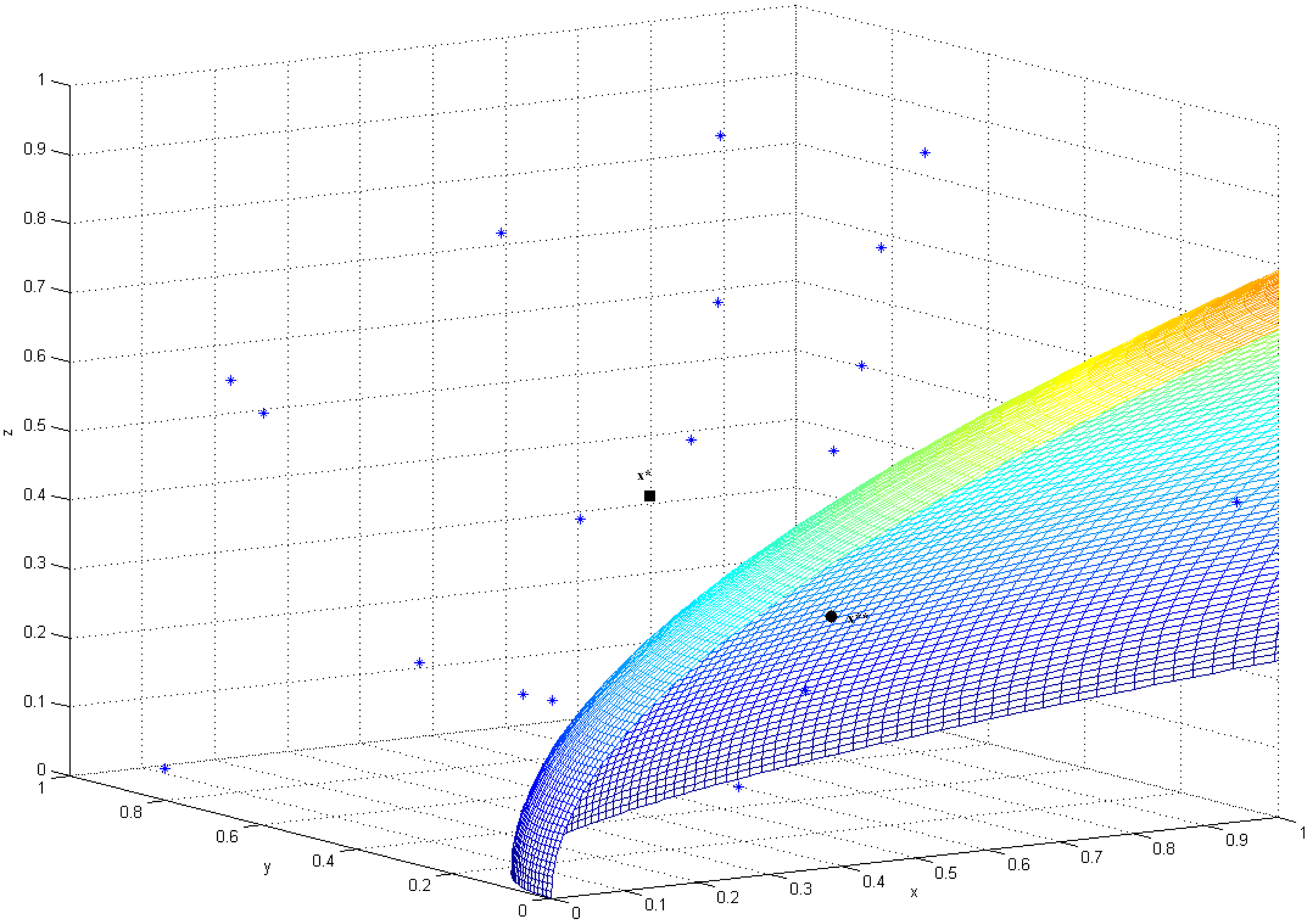
Figure 1. Feasible region, demand points and optimal solutions of Example 15.

In the following, we will apply this general methodology to get the reformulation of the most standard problems in Location Analysis (see Nickel and Puerto [25]) that will be later the basis of our computational experiments: minisum (Weber) and minimax (center), $k$-centrum, $(k_{1},k_{2})$-trimmed mean and range problems.

4.1. Weber or median problem

In the standard version of the Weber problem, we are given a set of demand points $\{a_{1},\ldots,a_{n}\}$ in $\mathbb{R}^{d}$ and a set of non-negative weights $\omega_{1},\ldots,\omega_{n}$ and one looks for a point $x^{*}$ minimizing the weighted Euclidean distance from the demand point. In other words, the problem is:

$$\min_{x\in\mathbb{R}^{d}}\sum_{i=1}^{n}\omega_{i}\|x-a_{i}\|_{2}.$$

This problem has been largely studied in the literature of Location Analysis and perhaps its most well-known algorithm is the so called Weiszfeld algorithm (see [38]). This problem is a convex one and Weiszfeld algorithm is a gradient type iterative algorithmic scheme for which several convergence results are known.

Here, we observe that this problem corresponds to a very particular choice of the elements in ($\mathbf{LOCOMRF}$): $\lambda=(1,\ldots,1)$, $f_{i}(u)=\omega_{i}u$ and $r=2$, $s=1$. Furthermore, the general formulation ($\mathbf{LOCOMRF}$) simplifies since there is no actual sorting. Therefore, we can avoid many of our instrumental variables, namely, the problem can be cast into the form:

$$\min \sum_{i=1}^{n}\omega_{i}z_{i}$$

$$s.t. \;z_{i}^{2}=\sum_{j=1}^{d}(x_{j}-a_{ij})^{2},i=1,\ldots,n,$$

($$\mathbf{WP} \displaystyle\sum_{j=1}^{d}x_{j}^{2}+z_{i}^{2}\leq M,i=1,\ldots,n,$$)

$$z_{i}\geq 0,\;i=1,\ldots,n,$$

$$x\in\mathbb{R}^{d}.$$

4.2. The minimax or center problem

The minimax location problem looks for the location of a server $x\in\mathbb{R}^{d}$ that minimizes the maximum weighted distance to a given set of demands points $\{a_{1},\ldots,a_{n}\}$ in $\mathbb{R}^{d}$. Formally, the problem can be stated as:

$$\min_{x\in\mathbb{R}^{d}}\max_{i=1,\ldots,n}\omega_{i}\|x-a_{i}\|_{2},$$

for some weights $\omega_{1},\ldots,\omega_{n}\geq 0$.

Once more, this problem has been extensively analyzed in the literature of Location Analysis and the most well-known algorithms to solve it are those by Elzinga-Hearn (only valid in $\mathbb{R}^{2}$ with Euclidean distance) and Dyer [8, 7] and Megiddo [23] which are polynomial in fixed dimension. Again, we observe that this problem corresponds to a very particular choice of the elements in ($\mathbf{LOCOMRF}$): $\lambda=(1,0,\ldots,0)$, $f_{i}(u)=\omega_{i}u$ and $r=2$, $s=1$. In this case, the general formulation ($\mathbf{LOCOMRF}$) simplifies and therefore, we can avoid many of our instrumental variables, namely, the problem can be formulated as:

$$\min \mbox{ }t$$

$$s.t. \;z_{i}^{2}=\sum_{j=1}^{d}(x_{j}-a_{ij})^{2},\;i=1,\ldots,n,$$

$$\omega_{i}z_{i}\leq t,\;i=1,\ldots,n,$$

($$\mathbf{CP} \sum_{j=1}^{d}x_{j}^{2}+z_{i}^{2}+t^{2}\leq M,\;i=1,\ldots,n,$$)

$$t,z_{i},\geq 0,\quad i=1,\ldots,n,$$

$$x\in\mathbf{K}.$$

4.3. The k-centrum problem

The $k$-centrum location problem consists of finding the point $x^{*}$ that minimizes the sum of the $k$ largest distances with respect to a given set of demands points $\{a_{1},\ldots,a_{n}\}$ in $\mathbb{R}^{d}$. Formally, the problem can be stated as:

$$\min_{x\in\mathbb{R}^{d}}\max_{i=1,\ldots,k}d_{(i)}(x),$$

where $d_{(i)}(x)=\|x-a_{\sigma(i)}\|$ for a permutation $\sigma$ such that $d_{\sigma(1)}(x)\geq\ldots\geq d_{\sigma(n)}(x)$. This problem has been considered in several papers and textbooks (see [25], [4]). Currently, there exist few approaches to solve it in the plane (i.e. $d=2$) and with the Euclidean norm that do not extend further to higher dimension nor other norms (see [5, 6, 34]). The objective function of this problem is described by a vector of $\lambda$-parameters $\lambda=(\overbrace{1,\ldots,1}^{k},0,\ldots,0)$, $f_{i}(u)=u$, $r=2$, $s=1$. Using the result in the reformulation (${\rm kC}$) the problem can be restated as:

$$\hat{\varrho}:= \min\;kt+\sum_{i=1}^{n}r_{i}$$

$$s.t.\;z_{i}^{2}=\sum_{j=1}^{d}(x_{j}-a_{ij})^{2},\;i=1,\ldots,n,$$

($$\mathbf{kCP} \qquad t+r_{i}\geq z_{i},\;i=1,\ldots,n,$$)

$$\qquad\sum_{j=1}^{d}x_{j}^{2}+z_{i}^{2}+r_{i}^{2}\leq M,\;i=1,\ldots,n,$$

$$\qquad t,r_{i},z_{i}\geq 0,\quad i=1,\ldots,n,$$

$$\qquad x\in\mathbb{R}^{d}.$$

4.4. The $(k_{1},k_{2})$-trimmed-mean problem

The $(k_{1},k_{2})$-trimmed-mean location problem looks for a point $x^{*}$ that minimizes the sum of the central distances, once we have excluded the $k_{2}$ closest and the $k_{1}$ furthest. Formally, the problem is:

$$\min_{x\in\mathbb{R}^{d}}\sum_{i=k_{1}+1}^{n-k_{2}}d_{(i)}(x),$$

where $d_{(i)}(x)=\|x-a_{\sigma(i)}\|_{2}$ for a permutation $\sigma$ such that $d_{\sigma(1)}(x)\geq\ldots\geq d_{\sigma(n)}(x)$. This problem has been considered in several papers and textbooks (see [25], [4]). Currently, there exists two approaches to solve it in the plane (i.e. $d=2$) and with the Euclidean norm that do not extend further to higher dimension nor other norms (see [5, 6]). The objective function of this problem, in terms of the elements in ($\mathbf{LOCOMRF}$), is described by a vector of $\lambda$-parameters $\lambda=(\overbrace{0,\ldots,0}^{k_{1}},1,\ldots,1,\overbrace{0,\ldots,0}^{k_{2}})$, $f_{i}(u)=u$, $r=2$, $s=1$. Here, we could apply the general formulation derived from ($\mathbf{LOCOMRF}$). Nevertheless, that approach needs many decision variables which affects the sizes of the problems to be handled. Rather than the general formulation, we present here an alternative problem, based on (${\rm kTr}$), which takes advantage of the particular structure of this problem and reduces the number of variables needed for its representation.

We consider the problem:

$$\min \;(n-k_{2})t+\sum_{i=1}^{n}r_{i}-\sum_{i=1}^{n}u_{i}z_{i}$$

$$s.t. \;z_{i}^{2}=\sum_{j=1}^{d}(x_{j}-a_{ij})^{2},\;i=1,\ldots,n,$$

$$\sum_{i=1}^{n}u_{i}=k_{1},$$

$$u_{i}(u_{i}-1)=0,\quad i=1,\ldots,n,$$

($$\mathbf{TMP} t+r_{i}\geq z_{i},\quad i=1,\ldots,n,$$)

$$\sum_{j=1}^{d}x_{j}^{2}+z_{i}^{2}+t^{2}+u_{i}^{2}+r_{i}^{2}\leq M,\;i=1,\ldots,n,$$

$$z_{i},r_{i},u_{i},t\geq 0,\quad i=1,\ldots,n,$$

$$x\in\mathbb{R}^{d}.$$

4.5. The range problem

The last problem that we address in our computational experiments is the range location problem. This problem consists of minimizing the difference (range) between the maximum and minimum distances with respect to a given set of demands points $\{a_{1},\ldots,a_{n}\}$ in $\mathbb{R}^{d}$ (see [5, 6, 25]). Formally, the problem can be stated as:

$$\min_{x\in\mathbb{R}^{d}}\left[\max_{i=1,\ldots,n}\|x-a_{i}\|_{2}-\min_{i=1,\ldots,n}\|x-a_{i}\|_{2}\right].$$

This problem corresponds to the following choice of the elements in ($\mathbf{LOCOMRF}$): $\lambda=(1,0,\ldots,0,-1),\;f_{i}(u)=u$ and $r=2$, $s=1$. A simplified reformulation of the problem reduces to:

$$\min \mbox{ }z-t$$

$$s.t. \;z_{i}^{2}=\sum_{j=1}^{d}(x_{j}-a_{ij})^{2},\;i=1,\ldots,n,$$

($$\mathbf{RP} t\leq z_{i}\leq z,\;i=1,\ldots,n,$$)

$$\sum_{j=1}^{d}x_{j}^{2}+z_{i}^{2}+t^{2}+z^{2}\leq M,\;i=1,\ldots,n,$$

$$t,z,z_{i}\geq 0,\quad i=1,\ldots,n,$$

$$x\in\mathbb{R}^{d}.$$

5. Computational Experiments

A series of computational experiments have been performed in order to evaluate the behavior of the proposed methodology. Programs have been coded in MATLAB R2010b and executed in a PC with an Intel Core i7 processor at 2x 2.93 GHz and 8 GB of RAM. The semidefinite programs have been solved by calling SDPT3 4.0[13].

We run the algorithm for several well-known continuous location problems: Weber problem, center problem, k-center problem, trimmed-mean problem and range problem. For each of them, we obtain the CPU times for computing solutions as well as the gap with respect to the optimal solution obtained with the battery of functions in optimset of MATLAB or the implementation by [5, 6].

With regard to computing the accuracy of an obtained solution, we use the following measure for the error (see [37]):

(12) $$\epsilon_{\rm obj}=\dfrac{|\text{the optimal value of the SDP }-{\rm fopt}|}{\max\{1,{\rm fopt}\}},$$

where ${\rm fopt}$ is the optimal objective value for the problem obtained with the functions in optimset or the implementation by [5, 6].

We have organized our computational experiments in five different problems types that coincide with those described previously in sections 4.1-4.5. Our test problems are generated to be comparable with previous results of some algorithms in the plane but, in addition, we also consider problems in $\mathbb{R}^{3}$. Thus, we report on randomly generated points on the unit square and in the unit cube. Depending on the problem, we have been able to solve different problem sizes. In all problems, we could solve instances with at least 500 points for planar and 3-dimensional problems and with an average accuracy higher than $10^{-5}$. (We remark that for instance we could solve instances of more than 1000 points for Weber and center problems with high precisions.)

Our goal is to present the results organized per problem type, framework space ($\mathbb{R}^{2}$ or $\mathbb{R}^{3}$) and relaxation order. We report for Weber problem on the first two relaxations to show that raising relaxation order one gains some extra precision (as expected) at the price of higher CPU times. In spite of that, the considered problems seems to be very well-approximated even with the first relaxation (as shown by our results). For this reason, we only report results for relaxation order $r=2$ for the remaining problem types, namely center, $k$-centrum, range and trim-mean.

The results in our tables, for each size and problem type, are the average of ten runs. In all cases our tables are organized in the same way. Rows give the results for the different number of demand points considered in the problems. Column n stands for the number of points considered in the problem, CPU time is the average running time needed to solve each of the instances, $\epsilon_{obj}$ gives the error measure (see 12). The final block of 3 columns informs on the sizes of the SDP problems to be solved: #Cols, #Rows and %NonZero represent, respectively, the number of columns, rows and the percentage of nonzero entries of the constraint matrices of the problems to be considered.

We tested problems with up to $500$ demands points (except for Weber problem where we considered $1000$ demands points) randomly generated in the unit square and the unit cube. We move n between $10$ and $500$ (or $1000$ for Weber problem) and ten instances were generated for each value of n. The first relaxation of the problems was solved in all cases. For the k-centrum problem type we considered three different $k$ values to test the difficulty of problems with respect to that parameter, $k=\lceil 0.1\texttt{n}\rceil,\lceil 0.5\texttt{n}\rceil,\lceil 0.9\texttt{n}\rceil$ (tables 4 and 5).

Tables 1-7 show the averages CPU times and gaps obtained. Table 1 summarizes the results of the Weber problems. We remark that problems with up to 1000 demand points on the plane are solved with the first relaxation in few seconds and with accuracy higher than $10^{-4}$. Raising the relaxation order, we improve accuracy till $10^{-6}$ at the cost of multiplying CPU time by a factor of 8. Table 2 refers to Weber problem in the $3d$ space. Results are similar although precision is higher when considering the second relaxation order. Table 3 reports the results for the center problem on the plane and the $3d$-space. CPU times are slightly larger than for the Weber problem but accuracy are also better specially for sizes up to 100 demand points. Tables 4 and 5 are devoted to show the behavior of our approach for three different $k$ values of the $k$-centrum problem (Table 4 in $\mathbb{R}^{2}$ and Table 5 in $\mathbb{R}^{3}$). We observe that for small values of $k$, i.e. $k=\lceil 0.1n\rceil\mbox{ or }\lceil 0.5n\rceil$ the $k$-centrum is slightly harder than for values closer to $n$. The remaining factors behave similarly to those in Weber or center problems. Table 6 reports the results for the range problem. The behavior of these problems is similar to that of the $k$centrum problems both in CPU time and accuracy. Finally, Table 7 summarizes the results for the trimmed-mean problems. These are the harder problems among the five considered problem types. We are able to solve similar sizes with similar accuracies using the first order relaxation. However, CPU times are significantly higher than for the other problem types. These results show that this methodology can be efficiently applied to solve medium to large sized location problems.

¿From our tables we conclude that Weber problem is the simplest one whereas the trimmed-mean problem is the hardest one, as expected. We remark that CPU times increase linearly with the number of points in all problem types. A linear regression between these times and the number of points gives a regression coefficient $R$-squared (coefficient of determination of the regression) greater than $0.98$ for all the problems. Therefore, this shows a linear dependence, up to the tested sizes, between problem sizes and CPU times for solving the corresponding relaxations. Observe that the sizes of the matrices in the SDP relaxations increase exponentially with the number of points. Nevertheless, the percentage of nonzero elements in the constraint matrices decreases very slowly (hyperbolically) when increasing the size (number of points) of the problems.

6. Conclusions

We develop a unified tool for minimizing weighted ordered averaging of rational functions. This approach goes beyond a trivial adaptation of the general theory of moments-sos since ordered weighted averages of rational functions are not, in general, neither rational functions nor the supremum of rational functions so that current results cannot directly be applied to handle these problems. As an important application we cast a general class of continuous location problems within the minimization of OWA rational functions. We report computational results that show the powerfulness of this methodology to solve medium to large continuous location problems.

This new approach solves a broad class of convex and non convex continuous location problems that, up to date, were only partially solved in the specialized literature. We have tested this methodology with some medium to large size standard ordered median location problems in the plane and in the 3-dimensional space. Our goal was not to compete with previous algorithms since most of them are either problem specific or only applicable for planar problems. However, in all cases we obtained reasonable CPU times and high accuracy results even with first relaxation order. Our good results heavily rely on the fact that we have detected sparsity patterns in these problems reducing considerably the sizes of the SDP object to be considered.

The two main lines for further research in this area would be to increase both the sizes and the classes of problems efficiently solved. These goals may be achieved by improving the efficiency of available SDP solvers and/or by finding alternative formulations that take advantage of new sparsity and symmetry patterns.

	First Relaxation ($r=2$)					Second Relaxation ($r=3$)
n	CPU time	$\epsilon_{\rm obj}$	#Cols	#Rows	%NonZero	CPU time	$\epsilon_{\rm obj}$	#Cols	#Rows	%NonZero
10	0.63	0.00191774	1420	214	0.780%	2.45	0.00008689	6200	587	0.279%
20	1.03	0.00079178	2840	414	0.403%	5.67	0.00002648	12400	1147	0.143%
30	1.03	0.00062061	4260	614	0.272%	8.94	0.00002065	18600	1707	0.096%
40	1.57	0.00082654	5680	814	0.205%	11.43	0.00000992	24800	2267	0.072%
50	2.12	0.00015842	7100	1014	0.165%	13.29	0.00000269	31000	2827	0.058%
60	2.31	0.00027699	8520	1214	0.137%	16.95	0.00000213	37200	3387	0.048%
70	2.72	0.00044228	9940	1414	0.118%	20.54	0.00000434	43400	3947	0.042%
80	3.03	0.00044249	11360	1614	0.103%	26.98	0.00000243	49600	4507	0.036%
90	3.38	0.00031839	12780	1814	0.092%	29.20	0.00000194	55800	5067	0.032%
100	3.92	0.00027367	14200	2014	0.083%	31.57	0.00000174	62000	5627	0.029%
150	6.12	0.00027644	21300	3014	0.055%	46.31	0.00000555	93000	8427	0.019%
200	8.36	0.00021865	28400	4014	0.042%	65.75	0.00000190	124000	11227	0.015%
250	10.42	0.00028088	35500	5014	0.033%	87.13	0.00000656	155000	14027	0.012%
300	12.19	0.00019673	42600	6014	0.028%	102.95	0.00001241	186000	16827	0.010%
350	14.63	0.00018747	49700	7014	0.024%	124.36	0.00000850	217000	19627	0.008%
400	17.25	0.00021381	56800	8014	0.021%	145.62	0.00000333	248000	22427	0.007%
450	20.37	0.00007970	63900	9014	0.019%	167.02	0.00000476	279000	25227	0.007%
500	22.03	0.00011803	71000	10014	0.017%	187.02	0.00000754	310000	28027	0.006%
600	28.11	0.00012725	85200	12014	0.014%	232.19	0.00000287	372000	33627	0.005%
700	33.47	0.00015215	99400	14014	0.012%	274.88	0.00000332	434000	39227	0.004%
800	39.50	0.00009879	113600	16014	0.010%	334.10	0.00000420	496000	44827	0.004%
900	45.31	0.00011740	127800	18014	0.009%	389.00	0.00000350	558000	50427	0.003%
1000	55.68	0.00012513	142000	20014	0.008%	443.13	0.00000351	620000	56027	0.003%

Table 1. Computational results for planar Weber problem and first and second relaxation.

	First Relaxation ($r=2$)					Second Relaxation ($r=3$)
n	CPU time	$\epsilon_{\rm obj}$	#Cols	#Rows	%NonZero	CPU time	$\epsilon_{\rm obj}$	#Cols	#Rows	%NonZero
10	1.19	0.00112213	2900	384	0.442%	9.13	0.00000379	17100	1343	0.124%
20	1.84	0.00036619	5800	734	0.231%	23.89	0.00000000	34200	2603	0.064%
30	2.56	0.00019790	8700	1084	0.157%	28.97	0.00000000	51300	3863	0.043%
40	3.54	0.00011433	11600	1434	0.118%	45.19	0.00000000	68400	5123	0.033%
50	4.27	0.00008446	14500	1784	0.095%	58.34	0.00000001	85500	6383	0.026%
60	5.04	0.00019406	17400	2134	0.080%	66.09	0.00000000	102600	7643	0.022%
70	6.23	0.00009027	20300	2484	0.068%	77.67	0.00000000	119700	8903	0.019%
80	7.09	0.00018689	23200	2834	0.060%	90.86	0.00000000	136800	10163	0.016%
90	8.01	0.00010943	26100	3184	0.053%	124.89	0.00000000	153900	11423	0.015%
100	9.87	0.00005552	29000	3534	0.048%	164.37	0.00000008	171000	12683	0.013%
150	14.16	0.00004856	43500	5284	0.032%	211.02	0.00000000	256500	18983	0.009%
200	20.33	0.00003049	58000	7034	0.024%	275.02	0.00000000	342000	25283	0.007%
250	25.97	0.00005964	72500	8784	0.019%	429.67	0.00000014	427500	31583	0.005%
300	34.00	0.00004677	87000	10534	0.016%	501.09	0.00000006	513000	37883	0.004%
350	39.82	0.00004154	101500	12284	0.014%	588.29	0.00000007	598500	44183	0.004%
400	47.27	0.00005233	116000	14034	0.012%	746.70	0.00000011	684000	50483	0.003%
450	57.08	0.00003325	130500	15784	0.011%	762.54	0.00000000	769500	56783	0.003%
500	65.93	0.00002952	145000	17534	0.010%	1063.50	0.00000000	855000	63083	0.003%

Table 2. Computational results for Weber problem in $\mathbb{R}^{3}$ and first and second relaxation.

	$\mathbb{R}^{2}$					$\mathbb{R}^{3}$
n	CPU time	$\epsilon_{\rm obj}$	#Cols	#Rows	%NonZero	CPU time	$\epsilon_{\rm obj}$	#Cols	#Rows	%NonZero
10	0.95	0.00000002	3150	384	0.423%	1.90	0.00000001	5700	629	0.259%
20	1.78	0.00000001	6300	734	0.221%	4.05	0.00000000	11400	1189	0.137%
30	2.68	0.00000001	9450	1084	0.150%	6.24	0.00000008	17100	1749	0.093%
40	3.78	0.00000001	12600	1434	0.113%	8.96	0.00000000	22800	2309	0.071%
50	4.68	0.00000000	15750	1784	0.091%	12.05	0.00000000	28500	2869	0.057%
60	6.05	0.00000000	18900	2134	0.076%	16.63	0.00000000	34200	3429	0.048%
70	8.48	0.00000000	22050	2484	0.065%	18.84	0.00000002	39900	3989	0.041%
80	10.28	0.00000002	25200	2834	0.057%	28.08	0.00000000	45600	4549	0.036%
90	13.60	0.00000005	28350	3184	0.051%	32.16	0.00000000	51300	5109	0.032%
100	18.86	0.00000005	31500	3534	0.046%	38.78	0.00000291	57000	5669	0.029%
150	31.12	0.00002157	47250	5284	0.031%	59.19	0.00006902	85500	8469	0.019%
200	38.76	0.00013507	63000	7034	0.023%	82.01	0.00011298	114000	11269	0.014%
250	44.34	0.00027776	78750	8784	0.019%	111.64	0.00013810	142500	14069	0.012%
300	58.10	0.00033715	94500	10534	0.015%	124.47	0.00030316	171000	16869	0.010%
350	81.59	0.00047225	110250	12284	0.013%	170.43	0.00043926	199500	19669	0.008%
400	90.22	0.00048347	126000	14034	0.012%	172.05	0.00052552	228000	22469	0.007%
450	93.50	0.00047479	141750	15784	0.010%	242.66	0.00057288	256500	25269	0.006%
500	151.64	0.00066416	157500	17534	0.009%	226.73	0.00059268	285000	28069	0.006%

Table 3. Computational results for center problem in $\mathbb{R}^{2}$ and $\mathbb{R}^{3}$ and first relaxations.

	$k=\lceil 0.1\,n\rceil$		$k=\lceil 0.5\,n\rceil$		$k=\lceil 0.9\,n\rceil$		Sizes
n	CPU time	$\epsilon_{\rm obj}$	CPU time	$\epsilon_{\rm obj}$	CPU time	$\epsilon_{\rm obj}$	#Cols	#Rows	#NonZero
10	2.64	0.00000630	2.76	0.00000081	2.59	0.00017665	6570	944	0.175%
20	6.43	0.00001375	6.15	0.00000298	5.30	0.00000545	13140	1854	0.089%
30	10.88	0.00000379	9.89	0.00000410	9.16	0.00000102	19710	2764	0.060%
40	15.89	0.00000717	16.33	0.00000090	12.22	0.00000122	26280	3674	0.045%
50	21.24	0.00000282	18.51	0.00000083	16.77	0.00000105	32850	4584	0.036%
60	25.77	0.00000077	25.41	0.00000283	20.21	0.00000806	39420	5494	0.030%
70	28.01	0.00000204	31.02	0.00000234	25.07	0.00000192	45990	6404	0.026%
80	37.25	0.00000085	31.48	0.00000044	30.66	0.00000220	52560	7314	0.023%
90	47.16	0.00000062	41.07	0.00000765	33.92	0.00000086	59130	8224	0.020%
100	53.68	0.00000084	41.42	0.00000065	39.49	0.00000188	65700	9134	0.018%
150	86.48	0.00000089	68.48	0.00000056	65.95	0.00000059	98550	13684	0.012%
200	123.02	0.00000056	96.40	0.00000075	88.10	0.00000275	131400	18234	0.009%
250	149.26	0.00003681	135.67	0.00000071	113.68	0.00000161	164250	22784	0.007%
300	180.38	0.00000408	161.84	0.00000081	146.22	0.00000349	197100	27334	0.006%
350	223.27	0.00003013	193.31	0.00003623	176.46	0.00000151	229950	31884	0.005%
400	260.27	0.00000079	225.07	0.00003689	201.01	0.00000376	262800	36434	0.005%
450	290.23	0.00004512	272.55	0.00000097	237.23	0.00000168	295650	40984	0.004%
500	345.93	0.00000224	310.19	0.00000119	269.99	0.00000200	328500	45534	0.004%

Table 4. Computational results for planar $k$-centrum problems and first relaxation ($r=2$).

	$k=\lceil 0.1\,n\rceil$		$k=\lceil 0.5\,n\rceil$		$k=\lceil 0.9\,n\rceil$		Sizes
n	CPU time	$\epsilon_{\rm obj}$	CPU time	$\epsilon_{\rm obj}$	CPU time	$\epsilon_{\rm obj}$	#Cols	#Rows	%NonZero
10	7.06	0.00041340	5.85	0.00000039	6.05	0.00000168	10780	1469	0.114%
20	16.40	0.00000950	15.42	0.00000095	16.30	0.00000019	21560	2869	0.059%
30	27.63	0.00001682	23.72	0.00000028	27.12	0.00000132	32340	4269	0.039%
40	45.25	0.00000075	42.31	0.00000086	37.38	0.00000077	43120	5669	0.030%
50	54.39	0.00000282	53.66	0.00000026	51.94	0.00000087	53900	7069	0.024%
60	63.16	0.00000259	59.34	0.00000091	63.91	0.00000065	64680	8469	0.020%
70	85.17	0.00000144	81.32	0.00000258	74.24	0.00000079	75460	9869	0.017%
80	106.65	0.00000326	83.96	0.00000044	88.76	0.00000158	86240	11269	0.015%
90	114.38	0.00000209	93.85	0.00000100	103.56	0.00000092	97020	12669	0.013%
100	122.01	0.00000088	109.17	0.00000224	118.03	0.00000067	107800	14069	0.012%
150	235.10	0.00000073	211.54	0.00000890	187.51	0.00000135	161700	21069	0.008%
200	305.51	0.00002407	255.54	0.00007106	284.80	0.00000157	215600	28069	0.006%
250	403.89	0.00000519	348.32	0.00004300	357.79	0.00000143	269500	35069	0.005%
300	492.04	0.00046130	433.69	0.00007630	471.78	0.00000174	323400	42069	0.004%
350	529.61	0.00041229	484.87	0.00000058	448.60	0.00001791	377300	49069	0.003%
400	619.97	0.00000091	585.93	0.00000055	523.81	0.00000829	431200	56069	0.003%
450	705.99	0.00048727	693.77	0.00000037	580.06	0.00004327	485100	63069	0.003%
500	817.75	0.00012138	789.77	0.00000087	664.94	0.00000318	539000	70069	0.002%

Table 5. Computational results for $k$-centrum problems in $\mathbb{R}^{3}$ and first relaxation ($r=2$).

	$\mathbb{R}^{2}$					$\mathbb{R}^{3}$
n	CPU time	$\epsilon_{\rm obj}$	#Cols	#Rows	%NonZero	CPU time	$\epsilon_{\rm obj}$	#Cols	#Rows	%NonZero
10	2.96	0.00007519	6060	629	0.252%	5.68	0.00001997	10080	965	0.164%
20	7.04	0.00001750	12120	1189	0.133%	18.45	0.00015758	20160	1805	0.088%
30	13.94	0.00098322	18180	1749	0.091%	35.37	0.00028187	30240	2645	0.060%
40	14.53	0.00002124	24240	2309	0.069%	35.77	0.00032049	40320	3485	0.045%
50	24.49	0.00004314	30300	2869	0.055%	65.80	0.00051293	50400	4325	0.037%
60	23.49	0.00047832	36360	3429	0.046%	59.19	0.00005082	60480	5165	0.031%
70	34.87	0.00003903	42420	3989	0.040%	68.46	0.00006841	70560	6005	0.026%
80	38.69	0.00026693	48480	4549	0.035%	79.54	0.00003016	80640	6845	0.023%
90	42.34	0.00042121	54540	5109	0.031%	90.76	0.00017468	90720	7685	0.021%
100	58.36	0.00052427	60600	5669	0.028%	97.26	0.00015535	100800	8525	0.019%
150	65.04	0.00021457	90900	8469	0.019%	159.41	0.00094711	151200	12725	0.012%
200	98.23	0.00041499	121200	11269	0.014%	197.66	0.00040517	201600	16925	0.009%
250	131.42	0.00033959	151500	14069	0.011%	274.14	0.00057559	252000	21125	0.007%
300	159.87	0.00014556	181800	16869	0.009%	322.21	0.00036845	302400	25325	0.006%
350	169.29	0.00003661	212100	19669	0.008%	393.80	0.00096204	352800	29525	0.005%
400	167.74	0.00123896	242400	22469	0.007%	361.12	0.00022448	403200	33725	0.005%
450	218.70	0.00207328	272700	25269	0.006%	513.55	0.00044016	453600	37925	0.004%
500	228.68	0.00438388	303000	28069	0.006%	554.94	0.00028013	504000	42125	0.004%

Table 6. Computational results for range problem in $\mathbb{R}^{2}$ and $\mathbb{R}^{3}$ and first relaxation.

	$\mathbb{R}^{2}$					$\mathbb{R}^{3}$
n	CPU time	$\epsilon_{\rm obj}$	#Cols	#Rows	%NonZero	CPU time	$\epsilon_{\rm obj}$	#Cols	#Rows	%NonZero
10	5.31	0.00017041	11760	1784	0.087%	14.09	0.00000197	18080	2669	0.059%
20	12.39	0.00000619	23520	3534	0.044%	33.85	0.00047792	36160	5269	0.030%
30	18.11	0.00020027	35280	5284	0.029%	49.16	0.00000670	54240	7869	0.020%
40	30.39	0.00035248	47040	7034	0.022%	73.13	0.00001450	72320	10469	0.015%
50	36.04	0.00181487	58800	8784	0.018%	98.17	0.00001624	90400	13069	0.012%
60	49.16	0.00085810	70560	10534	0.015%	131.38	0.00003143	108480	15669	0.010%
70	60.57	0.00012995	82320	12284	0.013%	161.25	0.00004420	126560	18269	0.009%
80	73.54	0.00092073	94080	14034	0.011%	188.51	0.00012265	144640	20869	0.008%
90	76.12	0.00040564	105840	15784	0.010%	203.06	0.00011847	162720	23469	0.007%
100	91.26	0.00218668	117600	17534	0.009%	220.68	0.00011032	180800	26069	0.006%
150	153.31	0.00814047	176400	26284	0.006%	400.37	0.00026203	271200	39069	0.004%
200	257.23	0.00032380	235200	35034	0.004%	552.19	0.00056138	361600	52069	0.003%
250	339.72	0.00051519	294000	43784	0.004%	659.01	0.00046219	452000	65069	0.002%
300	326.52	0.00225994	352800	52534	0.003%	884.40	0.00038481	542400	78069	0.002%
350	410.32	0.00047898	411600	61284	0.003%	955.53	0.00061467	632800	91069	0.002%
400	582.36	0.00047130	470400	70034	0.002%	1165.79	0.00058261	723200	104069	0.002%
450	631.58	0.00060180	529200	78784	0.002%	1931.76	0.00081711	813600	117069	0.001%
500	685.79	0.00079679	588000	87534	0.002%	9151.90	0.00063861	904000	130069	0.001%

Table 7. Computational results for trimmed mean problem with $k1=k2=\lceil 0.20\,n\rceil$ in $\mathbb{R}^{2}$ and $\mathbb{R}^{3}$ and first relaxation.

References

- [1] Blanquero R. and Carrizosa E. (2009). Continuous location problems and big triangle small triangle: constructing better bounds. J. Global Optim., 45 (3), 389–402.
- [2] Boland N., Domínguez-Marín P., Nickel S. and Puerto J. (2006). Exact procedures for solving the discrete ordered median problem. Computers and Operations Research, 33, 3270–3300.
- [3] Drezner Z. (2007). A general global optimization approach for solving location problems in the plane. J. Global Optim., 37 (2), 305–319.
- [4] Drezner Z. and Hamacher H.W. editors (2002). Facility Location: Applications and Theory. Springer.
- [5] Drezner Z., Nickel S. (2009). Solving the ordered one-median problem in the plane. European J. Oper. Res., 195 no. 1, 46–61.
- [6] Drezner Z., Nickel S. (2009). Constructing a DC decomposition for ordered median problems. J. Global Optim., 195 no. 2, 187–201.
- [7] Dyer M.E. (1986). On a multidimensional search procedure and its application to the Euclidean one-centre problem. SIAM J. Computing, 15, 725–738.
- [8] M.E. Dyer M.E. (1992). A class of convex programs with applications to computational geometry. Proceedings of the -th ACM Symposium on Computational Geometry, 9–15.
- [9] Espejo I., Marin A., Puerto J., Rodriguez-Chia A.M. (2009). A comparison of formulations and solution methods for the Minimum-Envy Location Problem, Computers and Operations Research, 36 (6), 1966–1981.
- [10] Jibetean D. and De Klerk E. (2006). Global optimization of rational functions: an SDP approach. Mathematical Programming, 106, 103–109.
- [11] Kalcsics J., Nickel S. andPuerto J. (2003). Multi-facility ordered median problems: A further analysis. Networks, 41 (1), 1–12, .
- [12] Kalcsics J., Nickel S., Puerto J., and Tamir A. (2002). Algorithmic results for ordered median problems defined on networks and the plane. Operations Research Letters, 30, 149–158, .
- [13] Kim-Chuan T., Michael J. Todd and Reha H. Tutuncu (2006). On the implementation and usage of SDPT3 - a MATLAB software package for semidefinite-quadratic-linear programming, version 4.0. Optimization Software, http://www.math.nus.edu.sg/ mattohkc/sdpt3/guide4-0-draft.pdf.
- [14] Krzemienowsk A., Ogryczak W. (2005).On extending the LP computable risk measures to account downside risk. Comput. Optim. Appl., 32 (2), 133–160.
- [15] Laraki R. and Lasserre J.B. (2010). Semidefinite Programming for min-max problems and Games. Mathematical Programming A. Published online, to appear.
- [16] Lasserre J. B. (2001). Global Optimization with Polynomials and the Problem of Moments. SIAM J. Optim., 11, 796–817.
- [17] Lasserre J.B. (2006). Convergent SDP-relaxations in polynomial optimization with sparsity. SIAM J. Optim., 17, 822–843.
- [18] Lasserre J. B. (2008). A semidefinite programming approach to the Generalized Problem of Moments. Mathematical Programming B, 112, 65–92.
- [19] Lasserre J.B. (2009). Moments and sums of squares for polynomial optimization and related problems. J. Global Optim., 45, 39–61.
- [20] Lasserre J.B. (2009). Moments, Positive Polynomials and Their Applications Imperial College Press, London.
- [21] López de los Mozos M.C., Mesa J.A. and Puerto J. (2008). A generalized model of equality measures in network. Computers and Operations Research, 35, 651–660, .
- [22] Marín A., Nickel S., Puerto J., and Velten S. (2009). A flexible model and efficient solution strategies for discrete location problems. Discrete Applied Mathematics, 157 (5), 1128–1145.
- [23] Megiddo N. (1989). On the ball spanned by balls. Discrete and Computational Geometry, 4, 605–610.
- [24] Nickel S. and Puerto J. (1999). A unified approach to network location problems. Networks, 34, 283–290, .
- [25] Nickel S. and Puerto J. (2005). Facility Location - A Unified Approach. Springer Verlag.
- [26] Ogryczak W. and Śliwiński T. (2010). On solving optimization problems with ordered average criteria and constraints. Stud. Fuzziness Soft Comput. Springer, Berlin, 254, 209–230.
- [27] Ogryczak W. (2010). Conditional median as a robust solution concept for uncapacitated location problems. TOP, 18 (1), 271–285.
- [28] Ogryczak W. and Śliviński T. (2009). On efficient WOWA optimization for decision support under risk. Internat. J. Approx. Reason., 50 (6), 915–928.
- [29] Ogryczak W. and Śliviński T. (2003). On solving linear programs with the ordered weighted averaging objective. European J. Oper. Res., 148 (1), 80–91.
- [30] Ogryczak W. and Zawadzki M. (2002). Conditional median: a parametric solution concept for location problems. Ann. Oper. Res., 110, 167–181.
- [31] Ogryczak W. and Ruszczyński A. (2002). Dual stochastic dominance and related mean-risk models. SIAM J. Optim., 13 (1), 60–78, .
- [32] Puerto J. and Tamir A. (2005). Locating tree-shaped facilities using the ordered median objective. Mathematical Programming, 102 (2), 313–338.
- [33] Putinar M. (1993). Positive Polynomials on Compact Semi-Algebraic Sets. Ind. Univ. Math. J., 42, 969–984.
- [34] Rodríguez-Chía A. M., Espejo I. and Drezner, Z. (2010). On solving the planar k-centrum problem with Euclidean distances. European J. Oper. Res., 207 (3), 1169–1186.
- [35] Schweighofer M. (2004). On the complexity of Schmüdgen’s Positivstellensatz. J. Complexity, 20, 529–543.
- [36] Schweighofer M. (2005). Optimization of polynomials on compact semialgebraic sets. SIAM J. Optim., 15, 805–825.
- [37] Waki H., Kim S., Kojima M., and Muramatsu M. (2006). Sums of Squares and Semidefinite Programming Relaxations for Polynomial Optimization Problems with Structured Sparsity. SIAM J. Optim., 17, 218–242.
- [38] Weiszfeld E. (1937). Sur le point pour lequel la somme des distances de n points donn s est minimum. Tohoku Math. Journal, 43, 355–386.
- [39] Yager R.R. (1988). On ordered weighted averaging aggregation operators in multicriteria decision making. IEEE Trans. Sys. Man Cybern., 18, 183–190, .
- [40] Yager R.R. (2009). Prioritized OWA aggregation. Fuzzy Optim. Decis. Mak., 8 (3), 245 -262.
- [41] Yager R.R. (2009). Using trapezoids for representing granular objects: applications to learning and OWA aggregation. Inform. Sci., 178 (2), 363 -380.
- [42] Yager R.R. (2004). Generalized OWA aggregation operators. Fuzzy Optim. Decis. Mak., 3 (1), 93 -107.
- [43] Yager R.R. (1996). Constrained OWA aggregation. Fuzzy optimization. Fuzzy Sets and Systems, 81 (1), 89 -101.
- [44] Yager R. and Kacprzyk J. (1997). The Ordered Weighted Averaging Operators: Theory and Applications, Kluwer: Norwell, MA.