Quantum dynamics of hard-core bosons in tilted bichromatic optical lattices

Abstract

We study the dynamics of strongly repulsive Bose gas in tilted or driven bichromatic optical lattices. Using the Bose-Fermi mapping and exact numerical method, we calculate the reduced single-particle density matrices, and study the dynamics of density profile, momentum distribution and condensate fraction. We show the oscillating and breathing mode of dynamics, and depletion of condensate for short time dynamics. For long time dynamics, we clearly show the reconstruction of system at integer multiples of Bloch-Zener time. We also show how to achieve clear Bloch oscillation and Landau-Zener tunnelling for many-particle systems.

I introduction

The dynamics of a particle in a period structure has been a fundamental subject, with the eigenenergies forming the famous Bloch bands Bloch1 and eigenstates being delocalized. If a weak external constant force is introduced, contrary to our intuition, the particle undergoes an oscillatory motion rather than uniform motion due to acceleration by the force, which is known as the famous Bloch oscillation Bloch1 ; Dahan1 . Under single-band tight-binding approximation, eigenenergies of the system form the Wannier-Stark ladder Gluck1 with eigenstates localized. Bloch oscillation bas been observed in semiconductor superlattices for electrons Feldmann1 , optical lattices for cold atoms Dahan1 and photonic crystals for light pluses Pertsch1 ; Morandotti1 . For a stronger force, a directed motion is re-introduced by repeated Landau-Zener tunneling to higher Bloch bands Landau1 ; Zener1 ; Majorana1 ; Stuckelberg1 . For usual cosine-shaped potentials, band gaps decrease rapidly as the energy increases, and this would lead to the decay of Bloch oscillation, which has been observed in Ref.Anderson1 ; Rosam1 ; Trompeter1 .

In order to study the interplay between Bloch oscillation and Landau-Zener tunneling, one needs at least a two-band system with the lowest two bands being well separated from upper ones. Furthermore, the gap between the lowest two Bloch bands must be small for observing clear signal of Landau-Zener tunneling. This can be achieved by bichromatic optical lattices Bloch2 , where parameters of the system are adjustable and controllable. Bichromatic lattices have been implemented by superimposing two incoherent optical lattices with the wavelength of one lattice being two times of the other Gorlitz1 ; Folling1 , or by virtual two-photon and four-photon processes Ritt1 ; Salger1 ; Salger2 ; Salger3 ; Kling1 . Under two-band tight-binding approximation, eigenenergies form two Wannier-Stark ladders with energy spacing doubled and an offset between them Breid1 ; Breid2 . The corresponding eigenstates are still localized. The dynamics of a particle is governed by two timescales, i.e., the Bloch period and the period of Zener oscillation. If the two periods are commensurate, system reconstructs at integer multiples of Bloch-Zener time.

So far, most of works concentrate on the dynamics of the single-particle system. The generalization of these results to interacting many-particle systems remains an open question. The possibility to investigate Bloch oscillation and Landau-Zener tunneling of interacting Bose-Einstein condensate (BEC) experimentally has attracted much interest. Most of theoretical studies are based on the mean-field approximation Wu1 ; Zobay1 ; Liu1 ; Graefe1 and Gross-Pitaevskii (GP) equations Witthaut1 . Results for the dynamics of strongly interacting many-particle systems are rarely known. In this paper, we study the dynamics of interacting bosons in bichromatic optical lattices under constant drag force in the limiting case with infinitely repulsive interaction which permits us to solve the problem exactly. The one-dimensional (1D) Bose gas with infinitely repulsive interaction is known as the hard-core boson (HCB) or Tonks-Girardeau (TG) gas Girardeau1 , which can be exactly solved via the Bose-Fermi mapping Girardeau1 and has attracted intensive theoretical attention Girardeau2 ; Minguzzi1 ; Gangardt1 . Experimental access to the required parameter regime has made the TG gas a physical reality Paredes1 ; Kinoshita1 . Following the exact numerical approach proposed by Rigol and Muramatsu Rigol1 ; Rigol2 , we calculate the dynamics of density profile, momentum distribution, and condensate fraction for hard-core bosons in the tilted bichromatic optical lattice, and show Bloch oscillation, Landau-Zener tunneling and reconstruction of the system at integer multiples of Bloch-Zener time.

The paper is organized as follows. In Section II, we present the model and the exact approach used in this paper. We also recover the dynamics of single particle system in this section. In Section III, we study the short-time and long-time dynamics for hard-core bosons in bichromatic optical lattice with a constant drag force. We also show how to achieve clear Bloch oscillation and Landau-Zener tunneling for the many-particle system. Finally, a summary is presented in Section IV.

II model and method

In the present section we describe the exact approach which we used to study 1D hard-core bosons in tilted or driven bichromatic optical lattices. Under the tight-binding approximation, the system can be described by the following Hamiltonian:

$$H= -J\sum_{i}(b^{\dagger}_{i}b_{i+1}+\mathrm{H.c.})+\delta\sum_{i}(-1)^{i}n^{b}_{i}$$ (1)

$$+F\sum_{i}in^{b}_{i}+\sum_{i}V_{i}n^{b}_{i}.$$

Here we only consider the nearest-neighbor hopping and neglect the off-diagonal terms of position operator $\hat{x}$ in the Wannier basis. The operator $b^{\dagger}_{i}$ ($b_{i}$) is the creation (annihilation) operator of boson which fulfills the hard-core constraints Rigol1 , i.e., the on-site anticommutation ($\{b_{i},b^{\dagger}_{i}\}=1$) and $[b_{i},b^{\dagger}_{j}]=0$ for $i\neq j$; $n^{b}_{i}$ is the bosonic particle number operator; $J$ is the hopping amplitude being set to be unit of energy ($J=1$); $V_{i}=V_{H}(i-i_{0})^{2}$ is the harmonic potential for preparing the initial state of system, with $V_{H}$ the strength and $i_{0}$ the position of the trap center; $\delta$ is the energy shift of alternate site; $F$ is the strength of driven force. For convenience, the lattice spacing is set to be unit.

In order to study the dynamics of the hard-core bosons in driven optical lattice, we first load the hard-core bosons into a bichromatic optical lattice with an additional harmonic trap, then we switch off the harmonic trap and turn on the driven force. We shall study the evolution of the initially prepared system and dynamics of the system under the driven force. First, the initial state is the ground state of Hamiltonian:

$$H_{\mathrm{init}}=-J\sum_{i}(b^{\dagger}_{i}b_{i+1}+\mathrm{H.c.})+\delta\sum_{i}(-1)^{i}n^{b}_{i}+\sum_{i}V_{i}n^{b}_{i},$$ (2)

with particle number $N$. In order to get the initial state, it is convenient to use the Jordan-Wigner transformation Jordan1 (JWT):

$$b^{\dagger}_{j}=f^{\dagger}_{j}\prod^{j-1}_{\beta=1}e^{-i\pi f^{\dagger}_{\beta}f_{\beta}},b_{j}=\prod^{j-1}_{\beta=1}e^{+i\pi f^{\dagger}_{\beta}f_{\beta}}f_{j},$$ (3)

to map the Hamiltonian of hard-core bosons into the Hamiltonian of noninteracting spinless fermions $H^{F}_{\mathrm{init}}$, which is in the same form as $H_{\mathrm{init}}$, but with all the boson operators, e.g.,$b^{\dagger}_{i}$, $b_{i}$ and $n^{b}_{i}$, being replaced by the corresponding fermion operators, e.g., $f^{\dagger}_{i}$, $f_{i}$ and $n^{f}_{i}$. The ground-state wave function of the system with $N$ spinless free fermions, which is a product of lowest N eigenfunctions, can be obtained by diagonalizing $H^{F}_{\mathrm{init}}$ and can be represented as

$$|\Psi^{G}_{F}\rangle=\prod^{N}_{n=1}\sum^{L}_{i=1}P_{in}f^{\dagger}_{i}|0\rangle,$$ (4)

where $L$ is the number of lattice sites, $N$ is the number of fermions (same as bosons), and coefficients $P_{in}$ are the amplitude of the $n$-th single-particle eigenfunction at $i$-th site which can form an $L\times N$ matrix $P$ Cai1 .

After releasing from the trap, the system is described by Hamiltonian:

$$H_{e}=-J\sum_{i}(b^{\dagger}_{i}b_{i+1}+\mathrm{H.c.})+\delta\sum_{i}(-1)^{i}n^{b}_{i}+F\sum_{i}in^{b}_{i}.$$ (5)

Similar to the above method, from the corresponding free-fermion Hamiltonian $H^{F}_{e}$, we can get all single-particle states and corresponding energies, and use $P^{\prime}$ to represent all the single-particle states, $\varepsilon_{i}$ to represent the energies. The nonequilibrium quantum dynamical properties of system can be calculated through the equal time one-particle Green function which is defined as:

$$G_{ij}(t)=\langle\Psi_{\mathrm{HCB}}(t)|b_{i}b^{\dagger}_{j}|\Psi_{\mathrm{HCB}}(t)\rangle,$$ (6)

with $|\Psi_{\mathrm{HCB}}(t)\rangle$ is the wave function of hard-core bosons at time $t$ after releasing from harmonic trap. After some derivations (see Appendix A), one can get

$$G_{ij}(t)=\det\left[\left(P^{A}\right)^{\dagger}P^{B}\right],$$ (7)

where $P^{A}$ and $P^{B}$ are obtained from $P$, $P^{\prime}$ and $\varepsilon_{i}$. It follows that the reduced single-particle density matrix can be determined by the expression

$$\rho_{ij}(t)=\langle b^{\dagger}_{i}b_{j}\rangle_{t}=G_{ji}(t)+\delta_{ij}(1-2G_{ii}(t)).$$ (8)

The momentum distribution is defined by Fourier transform with respect to $i-j$ of the reduced single-particle density matrix with the form

$$n(k)=\frac{1}{L}\sum^{L}_{i,j=1}e^{-ik(i-j)}\rho_{ij}$$ (9)

where $k$ denotes momentum. The natural orbitals $\phi^{\eta}_{i}$ are defined as eigenfunctions of the reduced single-particle density matrix Pensose1 ,

$$\sum^{L}_{j=1}\rho_{ij}\phi^{\eta}_{j}=\lambda_{\eta}\phi^{\eta}_{i}.$$ (10)

The natural orbitals can be understood as being effective single-particle states with occupations $\lambda_{\eta}$. For noninteracting bosons, all particles occupy in the lowest natural orbital and bosons are in the BEC phase at zero temperature, whereas only the quasicondensation exists for 1D hard-core bosons Rigol1 .

For hard-core bosons we know that the state for the corresponding Fermi Hamiltonian is a product of time-dependent single-particle states and each single-particle state evolves itself (see Eq.(16) in Appendix A). We recover the single-particle properties of the Hamiltonian $H_{e}$ in Appendix B, which have been studied by Breid et. al Breid1 . From Appendix B, we know that a single-particle wave function will be reconstructed at integer multiples of Bloch-Zener time ($T_{\mathrm{BZ}}$), if $T_{1}$ and $T_{2}$ are commensurate. Here $T_{1}$ is the Bloch period decided by the spacing of Wannier-Stark ladders, and $T_{2}$ is the period of Zener oscillation decided by the offset between Wannier-Stark ladders. Since each single-particle state can be reconstructed at period of time, and the period is independent of the single-particle state and decided by parameters of Hamiltonian, the state for many-body hard-core bosons composed of a product of single-particle states will also be reconstructed at integer multiples of Bloch-Zener time.

III quantum dynamics of hard-core bosons

In order to observe reconstruction of system, two periods $T_{1}$ and $T_{2}$ must be commensurate which are decided by $F$ and $E_{0}$, where $E_{0}$ is a function of $F$ and $\delta$. In Fig.1a, we show numerical results of $E_{0}$ versus $\delta$ for a particular $F$. For different $F$, structure of the picture is similar. In order to generate particular Bloch-Zener time ($T_{\mathrm{BZ}}$), $\delta$ must be one of the discrete numbers. For example, if we want $T_{\mathrm{BZ}}=T_{B}$ for the system with $F=0.05$, we have to let $E_{0}=0$ and then $\delta=0.1684,0.3614,...$.

For comparison, we first recover the dynamics of a single particle system. We choose $E_{0}=0$ and let system reconstruct at integer multiples of Bloch time ($T_{B}$). From now on, we take Bloch time $T_{B}=2T_{1}$ as the reference timescale. In Fig.1b, we show the dynamical evolution of density profile for a single-particle system, from which one can see the reconstruction of the density profile at integer multiples of Bloch time. The edge of Brillouin zone is reached at $t=T_{B}/4$, and part of particle moves into upper excited Bloch band located in upper half of the figure. The particle in upper excited band returns to lower Bloch band at $t=3T_{B}/4$. For quantitative analysis of Landau-Zener tunneling rate, one can characterize it by the number of particles in upper half of picture at time $t=T_{B}/2$. Numerical results show that the Landau-Zener tunnelling probability Witthaut1 :

$$P_{\mathrm{LZ}}\approx\mathrm{exp}(-\frac{\pi\delta^{2}}{2F}).$$ (11)

So in order to see a clear signal of Landau-Zener tunneling, we have to choose small $\delta$ for a given strength of force $F$. Furthermore, the available interval for motion of a particle in lattice Hartmann1 :

$$L\approx 4/F.$$ (12)

In Fig.1c, we also show the dynamical evolution of momentum distribution of the single-particle system. Particles with momentum in the interval $(-\pi/2,\pi/2)$ are in lower Bloch band and outside the region particles are in upper excited Bloch band. From this picture we can see the clear signals for Bloch oscillation and Landau-Zener tunneling. Furthermore the momentum is linear with time with slope given by $F$. Next we consider a localized initial state which has a wide momentum distribution and can be implemented by setting a strong harmonic trap potential, for example, $V_{H}=20$ here. From Fig.1d, one can find a breathing behavior of density profile. The reconstruction still happens at integer multiples of $T_{B}$. But one can observe that the enveloping structure with period of $T_{B}$ is overlayed by a breathing mode of smaller amplitude, whereas part of particle remains in lower Bloch band all the time with period of $T_{B}/2$.

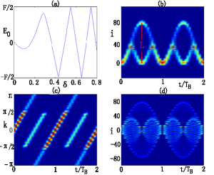
Figure 1: (Color online) (a): $E_{0}$ vs $\delta$ for the system with $F=0.05$. The dynamics of density profile (b) and momentum distribution(c) for single particle system with $\delta=0.1684$, $F=0.05$, and $V_{H}=0.001$. (d): The breathing mode dynamics of density profile for single particle system with $\delta=0.1684$, $F=0.05$, and $V_{H}=20$.

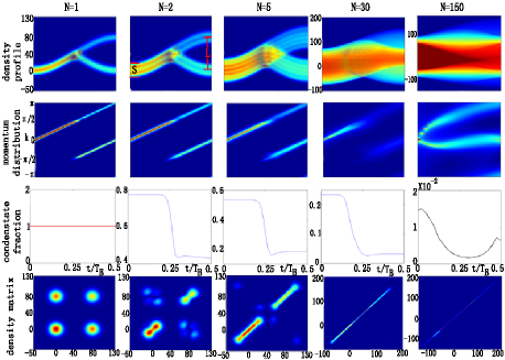
Figure 2: (Color online) The short-time dynamical evolution of density profile (first row), momentum distribution (second row), condensate fraction (third row), and modules of the reduced single-particle density matrix (fourth row) at time $t=T_{B}/2$ for systems of different particle number with $F=0.05$, $\delta=0.1684$, $E_{0}=0$, and $V_{H}=10^{-4}$ ($V_{H}=8\times 10^{-4}$ for the fifth column).

Now we consider the case of many-body hard-core bosons and study the short time dynamics firstly. Systems with various particle numbers will be considered by keeping the other parameters fixed. For comparison, we show the dynamics of a single-particle system in the first column of Fig.2. After releasing from trap, the particle speeds up under the drag force $F$, and it reaches the edge of Brillouin zone at time $T_{B}/4$. Part of particle moves into upper excited Bloch band through Landau-Zener tunneling, while the other part of particle remains in lower Bloch band with changing of sign of momentum by Brag scattering. Because of Landau-Zener tunneling, the particle turns into two parts and they are separated in the real space with particles in the upper half of the density distribution being in the upper excited Bloch band. In momentum distribution, the particles outside the first Brillouin zone of ($-\pi/2,\pi/2$) are in upper excited Bloch band. The changing of sign of momentum occurs at time $T_{B}/4$ by Brag scattering for particles in the lower Bloch band. In the third row of Fig.2, we show the evolution of condensate fraction which is defined as $\lambda_{0}/N$ with $\lambda_{0}$ being the occupation of the lowest effective single-particle state. For single particle system, the particle is always in the lowest effective single-particle state, and the condensate fraction is one all the time. For the 1D many-body systems of hard-core bosons, there are only quasi-condensation with $\lambda_{0}\propto\sqrt{N}$ Girardeau1 ; Rigol1 . In the fourth row of Fig.2, we show the reduced single-particle density matrix at time $T_{B}/2$. Here we consider the modulus because of the elements of density matrix being complex numbers after turning off trap. The upper right spot in picture is caused by particles in upper excited Bloch band and the lower left spot for lower Bloch band. For single particle dynamics, however particles in upper excited Bloch band and lower Bloch band are separated in real space, there are phase coherence between them, the off-diagonal parts of reduced single-particle density matrix are very strong.

In the second to fifth column, we show the dynamics for the hard-core bosons with $N=2,5,30$ and $150$, respectively. As particle number increases, the adding particle has to occupy higher single-particle state because one state can only be occupied by a hard-core boson. And the size ($S$) of system becomes larger and larger, while the available interval $L$ of the system decided by force $F$ remains unchanged. Also, the width of momentum distribution becomes wider for the larger system. As the momentum distribution becomes wider, it takes shorter time for particles at the edge of the momentum distribution to reach the edge of Brillouin zone, and thus Landau-Zener tunneling happens early, which leads to the condensate fraction decreasing early. The condensate fraction decreases ($\propto 1/\sqrt{N}$) as the particle number increases. As time increases but is smaller than $T_{B}/4$, the condensate fraction basically does not change. A slight increase of the condensate fraction in short time is caused by the expanding after turning off trap Cai1 . At time $t=T_{B}/4$, Landau-Zener tunneling happens, and the condensate fraction decreases quickly. After this there appears an overdamped area, and then the condensate fraction keeps unchanged basically. For the reduced single-particle density matrix at time $T_{B}/2$, lengths for the two parts of diagonal terms become larger as the size ($S$) of system increases. The off-diagonal parts of matrix become weaker as particles add in. Also, the phase coherence between particles in the upper excited Bloch band and lower Bloch band decreases. As shown in the figure, the particles between upper band and lower band lost their phase coherence when $N=30$. Furthermore, the particles in the upper excited Bloch band and lower Bloch band developed phase coherence inside each part, the reduced single-particle density matrix has exponential-law decay in each part as the distance increases.

We note that the density profile no longer splits into two obviously separated parts after time $T_{B}/4$ for system with $N=30$ as shown in the fourth column, where the particles in the upper excited Bloch band and lower Bloch band are overlapped in real space. To achieve this situation, one has to adjust the parameters of system and let the size of system larger than the available interval ($S>L$). Also one has to avoid the initial state staying in a localized state because localized initial state will cause the breathing-mode dynamics. Although the two parts are overlapped in real space, they are separated in the momentum distribution. The width of the momentum distribution becomes larger as the particle number increases. The dynamical evolution of condensate fraction still has similar structure, except that the quick decrease happens more early. As two parts of particles are overlapped in real space, the diagonal terms of density matrix are also overlapped. For sites outside the overlapped area in upper excited Bloch band or lower one, the density matrix still has a exponential-law decay as distance increases. For overlapped area, the density matrix is irregular, but as the distance increases, it goes to zero quickly. In the fifth column, we show the dynamics of system with $N=150$. As the particle number increases, the localization of initial state becomes stronger Rigol1 , and we see the breathing mode of dynamics of density distribution. Lots of particles are localized in the center, and particles in two parts are overlapped. The dynamics of momentum distribution is also changed. The momentum distribution does not increase linearly as time increases, and momentum distributions for particles in the upper excited Bloch band and lower Bloch band are overlapped. For localized initial state, the momentum distribution is almost flat. Right after turning off trap, there are particles moving into upper excited Bloch band through Landau-Zener tunnelling, and the condensate fraction decreases immediately. Meanwhile, for a localized initial state, the expanding is also important after turning off trap, and there is a large overdamped area in the breathing mode dynamics of condensate fraction. The reduced single-particle density matrix still has exponential-law decay for particles in localized states.

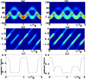
Figure 3: (Color online) The dynamical evolution of density profile (a,d), momentum distribution (b,e), and condensate fraction (c,f) for five-particle system with $F=0.05$, $V_{H}=10^{-3}$ and $\delta=0.1684$ (a,b,c), $\delta=0.238$ (d,e,f).

Next, we consider the long-time dynamics of hard-core bosons. In Fig.3a, we show the dynamical evolution of density distribution for five-particle system with Bloch-Zener time $T_{\mathrm{BZ}}=T_{B}$, where $E_{0}=0$. After releasing from the harmonic trap, particles move along with the direction of the force $F$. Around time $t=T_{B}/4$, particles reach the edge of Brillouin zone, and part of particles move into the upper excited Bloch band through Landau-Zener tunneling and keep moving along with force $F$. The other part of particles remain in the lower Bloch band, but the momentum of particles changes the sign due to Brag scattering and thus the particles move against the force $F$. Around time $t=3T_{B}/4$, particles reach the edge of Brillouin zone again, and all particles move into the lower Bloch band. At time $t=T_{B}$, the system reconstructs into the initial state. As time goes on, more periods occur. The dynamical evolution of the momentum distribution for the same system is shown in Fig.3b. After turning off trap, particles accelerate under force $F$, and the momentum increases linearly with time. Around time $t=T_{B}/4$, particles reach the edge of Brillouin zone ($k=\pi/2$). Part of particles, which move into the upper Bloch band through Landau-Zener tunnelling, remain in the same belt and their momentum increases linearly with time. The other part of particles keep in the lower Bloch band and change the sign of their momentum by Brag scattering. Two parts of particles are recombined around time $t=3T_{B}/4$, and the momentum distribution returns to the initial distribution at $t=T_{B}$. In Fig.3c, we show the dynamical evolution of condensate fraction. Around time $t=T_{B}/4$, the condensate fraction has a quick decrease due to Landau-Zener tunneling. After this there is an overdamped area. Around time $t=3T_{B}/4$, two parts of particles recombine, and the condensate fraction increases quickly. The system returns to its initial state at time $T=T_{\mathrm{BZ}}$. Furthermore, the condensate fraction is symmetrical with center at $T=T_{\mathrm{BZ}}/2$. In Fig.3, we also show the dynamics of system with $T_{\mathrm{BZ}}=2T_{B}$ where $E_{0}=F/4$, which has similar properties with the previous one. From Fig.3d, one can obviously observe the reconstruction of system after Bloch-Zener time $T_{\mathrm{BZ}}$, Bloch oscillation and Landau-Zener tunneling.

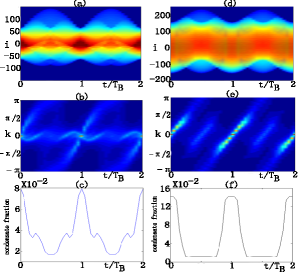
Figure 4: (Color online) The dynamical evolution of density profile (a,d), momentum distribution (b,e), and condensate fraction (c,f) for the eighty-particle system with $F=0.05$, $\delta=0.1684$ and $V_{H}=10^{-3}$ (a,b,c), $V_{H}=4\times 10^{-5}$ (d,e,f).

In Fig.4, we show the dynamical evolution of system with eighty hard-core bosons. As particles add in, the particles in the initial state get more localized, and the dynamical evolution of the system is dominated by the breathing mode instead of the oscillating mode. In Fig.4a, we show the dynamical evolution of the density profile for system with $F=0.05$, $\delta=0.1684$ and $V_{H}=10^{-3}$. This picture is not in prefect breathing mode because of the initial state being not localized enough. First of all, the reconstruction of density profile happens again after integer multiples of Bloch-Zener time $T_{\mathrm{BZ}}$. Second, lots of particles are localized at the center and form a belt. Third, one can observe that the enveloping structure is overlayed by a breathing mode of smaller amplitude. The outside breathing mode is formed by Bloch oscillation and Landau-Zener tunneling for particles in the upper excited Bloch band with period $T_{\mathrm{BZ}}=T_{B}$. The inside breathing mode is formed by Bloch oscillation for particles remaining in the lower Bloch band with period $T_{1}=T_{B}/2$. Center is the localized belt. In Fig.4b we show the dynamical evolution of the momentum distribution. Strip structure disappears and windmill structure appears with the center at $(nT_{B},k=0)(n\in\mathbb{N})$. In this picture we can not distinguish the two parts of particles, and lots of particles are localized at area of $k\approx 0$ all the time. Foremost, the momentum distribution reconstructs at integer multiples of $T_{\mathrm{BZ}}$. The dynamical evolution of the condensate fraction is shown in Fig.4c, As the initial state is a localized state, there are many particles with high momentum, and right after turning off trap the condensate fraction decreases quickly, and it reconstructs at $t=T_{\mathrm{BZ}}$. As a lot of particles add in, the initial state becomes a localized state and one can observe breathing mode dynamical evolution of density profile. In order to observe the oscillating mode and Landau-Zener tunneling, we have to reduce the localization of initial state by decreasing the strength of the harmonic trap. The dynamics of system after decreasing the strength of trap is shown in the second column of Fig.4. For the density distribution we actually see the oscillating mode, but we can not see the Landau-Zener tunneling clearly. At time range $(T_{B}/4,3T_{B}/4)$, the particles in the upper excited Bloch band and lower Bloch band are overlapped in real space. This is due to the available interval for the motion being $L\approx 4/F=80$ for system with $F=0.05$, but the size of system is about $S\approx 300$. It is clear that $S>L$ and the overlapped structure appears. After decreasing the strength of trap, the strip structure reappears in the dynamical evolution of the momentum distribution instead of the windmill structure. Furthermore the momentum distribution between the particles in the upper excited and lower Bloch band are distinguishable despite they are overlapped in real space. For the condensate fraction, the curve is flat again for the time short after turning off trap.

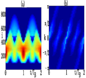
Figure 5: (Color online) The dynamical evolution of density profile (a), momentum distribution (b), for the eighty-particle system with $F=0.01$, $\delta=0.08211$ and $V_{H}=4\times 10^{-5}$.

So in order to observe the oscillating mode of dynamics and Landau-Zener tunneling, one has to let $L>S$. Now we have to decrease the strength of force $F$ to achieve a bigger available interval for the motion. Once $F$ is changed , we have to change $\delta$ too to make $E_{0}=0$ for the system still with Bloch-Zener time $T_{\mathrm{BZ}}=T_{B}$. Furthermore we have to choose a small $\delta$ to achieve the big enough Landau-Zener tunneling probability, otherwise we only see the Bloch oscillation but can not see the Landau-Zener tunneling. In Fig.5a, we show the dynamical evolution of density profile for the system with $F=0.01$, $\delta=0.08211$ and $T_{\mathrm{BZ}}=T_{B}$. Now we see the clear signals of Bloch oscillation and Landau-Zener tunneling. The dynamical evolution of the momentum distribution and condensate fraction are similar to Fig.4e and Fig.4f.

IV conclusion

In summary, we have studied the dynamics of infinitely repulsive Bose gas in tilted or driven bichromatic optical lattices. Using the Bose-Fermi mapping and exact numerical method, we calculate the one-particle density matrices, density profiles, momentum distributions, natural orbitals and their occupations (condensate fraction). Both the short-time and long-time dynamical evolution of density profile, momentum distribution and condensate fraction are studied. It is clearly shown that the reconstruction of system at integer multiples of Landau-Zener time. We also give estimations for how to achieve clear Bloch oscillation and Landau-Zener tunneling in given many-particle systems.

Appendix A THE EQUAL TIME GREEN FUNCTION FOR HARD-CORE BOSONS

The equal time Green function for the hard-core bosons can be written in the form

$$G_{ij}(t) = \langle\Psi_{\mathrm{HCB}}(t)|b_{i}b^{\dagger}_{j}|\Psi_{\mathrm{HCB}}(t)\rangle$$ (13)

$$= \langle\Psi_{F}(t)|\prod_{\beta=1}^{i-1}e^{i\pi f^{\dagger}_{\beta}f_{\beta}}f_{i}f^{\dagger}_{j}\prod_{\gamma=1}^{j-1}e^{-i\pi f^{\dagger}_{\gamma}f_{\gamma}}|\Psi_{F}(t)\rangle$$

$$= \langle\Psi^{B}|\Psi^{A}\rangle$$

where $|\Psi_{\mathrm{HCB}}(t)\rangle$ is the wave function of hard-core bosons at time $t$ after releasing from harmonic trap and $|\Psi_{F}(t)\rangle$ is the corresponding one for noninteracting fermions. In addition, we denote

$$\left|\Psi^{A}\right\rangle = f^{\dagger}_{j}\prod_{\gamma=1}^{j-1}e^{-i\pi f^{\dagger}_{\gamma}f_{\gamma}}|\Psi_{F}(t)\rangle,$$

$$\left|\Psi^{B}\right\rangle = f^{\dagger}_{i}\prod_{\beta=1}^{i-1}e^{-i\pi f^{\dagger}_{\beta}f_{\beta}}|\Psi_{F}(t)\rangle.$$ (14)

The wave function $|\Psi_{F}(t)\rangle$ can be easily calculated with the initial wave function $|\Psi^{G}_{F}\rangle$

$$|\Psi_{F}(t)\rangle=e^{-iH^{F}_{e}t}|\Psi^{G}_{F}\rangle=\prod_{n=1}^{N}\sum_{l=1}^{L}P_{ln}(t)f_{l}^{\dagger}|0\rangle,$$ (15)

with

$$P_{ln}(t)=\sum^{N}_{k=1}e^{-i\varepsilon_{k}t}P^{\prime}_{lk}\sum^{N}_{j=1}(P^{\prime*}_{jk}P_{jn}),$$ (16)

where we have set $\hbar=1$ in evolution operator, and $P(t)$ is the matrix of $|\Psi_{F}(t)\rangle$ in the same way as $|\Psi^{G}_{F}\rangle$. In order to get Eq.(15), one has to insert $\sum_{j=1}^{L}|\phi_{j}\rangle\langle\phi_{j}|=1$ in to it, where $|\phi_{j}\rangle=\sum_{n=1}^{L}P^{\prime}_{nj}f^{\dagger}_{n}|0\rangle$ is the lowest j-th eigenfunction of $H^{F}_{e}$.We can see that $|\Psi_{F}(t)\rangle$ is still a product of time-dependent single-particle states.

In order to calculate $\Psi^{A}$(and $\Psi^{B}$) we notice that

$$\prod_{\gamma=1}^{j-1}e^{-i\pi f^{\dagger}_{\gamma}f_{\gamma}}=\prod_{\gamma=1}^{j-1}[1-2f^{\dagger}_{\gamma}f_{\gamma}].$$ (17)

Then, the action of $\prod_{\gamma=1}^{j-1}e^{-i\pi f^{\dagger}_{\gamma}f_{\gamma}}$ on the state $|\Psi_{F}(t)\rangle$ (Eq.(15)) generates only a change of sign on the element $P_{ln}(t)$ for $l<j$, and one has to add a column to $P(t)$ with element $P_{j,N+1}=1$ and all the others equal to zero for the further creation of a particle at site j. Then

$$\left|\Psi^{A}\right\rangle = \prod_{n=1}^{N+1}\sum_{l=1}^{L}P_{ln}^{A}f_{l}^{\dagger}\left|0\right\rangle$$

$$\left|\Psi^{B}\right\rangle = \prod_{n=1}^{N+1}\sum_{l=1}^{L}P_{ln}^{B}f_{l}^{\dagger}\left|0\right\rangle$$ (18)

where $P^{A}$ and $P^{B}$ are obtained from $P(t)$ changing the required signs and adding the new column.

The Green function is written as

$$G_{ij}(t) = \langle 0|\prod_{n=1}^{N+1}\sum_{l=1}^{L}P^{B*}_{ln}f_{l}\prod_{n^{\prime}=1}^{N+1}\sum_{l^{\prime}=1}^{L}P^{A}_{ln}f_{l}^{\prime}|0\rangle$$ (19)

$$= \sum_{l_{1}\cdot\cdot\cdot 1_{N+1},l^{\prime}_{1}\cdot\cdot\cdot 1^{\prime}_{N+1}}^{L}P^{B*}_{l_{1}1}\cdot\cdot\cdot P^{B*}_{l_{N+1}N+1}$$

$$\times P^{A}_{l^{\prime}_{1}1}\cdot\cdot\cdot P^{A}_{l^{\prime}_{N+1}N+1}\langle 0|f_{l_{1}}\cdot\cdot\cdot f_{l_{N+1}}f^{\dagger}_{l^{\prime}_{l_{N+1}}}\cdot\cdot\cdot f^{\dagger}_{l^{\prime}_{1}}|0\rangle$$

$$= \mathrm{det}[(P^{B})^{\dagger}P^{A}]$$

which requires

$$\langle 0|f_{l_{1}}\cdot\cdot\cdot f_{l_{N+1}}f^{\dagger}_{l^{\prime}_{l_{N+1}}}\cdot\cdot\cdot f^{\dagger}_{l^{\prime}_{1}}|0\rangle=$$ (20)

$$\varepsilon^{\lambda_{1}\cdot\cdot\cdot\lambda_{N+1}}\delta_{l_{1}l^{\prime}_{\lambda_{1}}}\cdot\cdot\cdot\delta_{l_{N+1}l^{\prime}_{\lambda_{N+1}}}$$

with $\varepsilon^{\lambda_{1}\cdot\cdot\cdot\lambda_{N+1}}$ the Levi-Civita symbol and $\lambda=1\cdot\cdot\cdot N+1$.

Appendix B THE SINGLE-PARTICLE PROPERTIES OF HAMILTONIAN $H_{e}$

First of all, for the field-free case with $F=0$, a straightforward calculation yields the dispersion relation

$$E_{\beta k}=(-1)^{\beta+1}\sqrt{\delta^{2}+4\mathrm{cos}^{2}(k)},$$ (21)

and corresponding wavefunctions $|\chi_{\beta}(k)\rangle$ (Bloch bands and Bloch waves) with the miniband index $\beta=0,1$. For nonzero F, the spectrum of Hamiltonian consists of two Wannier-Stark ladders with an offset in between. After introducing translation operator

$$T_{m}=\sum^{\infty}_{n=-\infty}b^{\dagger}_{n-m}b_{n}$$ (22)

and an operator $G$ that causes the inversion of sign of $\delta$ in Hamiltonian:

$$GH_{e}(\delta)=H_{e}(-\delta)G,\quad\quad[T_{m},G]=0,$$ (23)

an eigenvector $|\Psi\rangle$ of $H_{e}$ with the eigenvalue $E(\delta,F)$ satisfies:

$$H_{e}\{T_{2l}|\Psi\rangle\}=\{E(\delta,F)-2lF\}\{T_{2l}|\Psi\rangle\}$$ (24)

$$H_{e}\{T_{2l+1}|\Psi\rangle\}=\{E(-\delta,F)-(2l+1)F\}\{T_{2l+1}|\Psi\rangle\}.$$

Thus, the eigenenergies of Hamiltonian

$$E_{0,n} = E(\delta,F)+2nF$$

$$E_{1,n} = E(-\delta,F)+(2n+1)F,$$ (25)

consists of two Wannier-Stark ladders with the corresponding eigenstates $|\Psi_{\beta,n}\rangle=T_{-(2n+\beta)}G^{\beta}|\Psi\rangle$ Breid1 . A further calculation can prove that $E_{0}\equiv E(\delta,F)=-E(-\delta,F)$.

For an initial state expanded in Wannier-Stark basis:

$$|\Phi\rangle=\sum_{n}c_{0,n}|\Psi_{0,n}\rangle+\sum_{n}c_{1,n}|\Psi_{1,n}\rangle,$$ (26)

the dynamics of $|\Phi\rangle$ under Hamiltonian $H_{e}$ is given by

$$|\Phi(t)\rangle=\sum_{n}c_{0,n}e^{-iE_{0,n}t}|\Psi_{0,n}\rangle+\sum_{n}c_{1,n}e^{-iE_{1,n}t}|\Psi_{1,n}\rangle.$$

Expanding Wannier-Stark functions in Bloch basis:

$$|\Psi_{\beta,n}\rangle=\int^{\tfrac{\pi}{2}}_{-\tfrac{\pi}{2}}a_{\beta n}(k)|\chi_{0}(k)\rangle\mathrm{d}k+\int^{\tfrac{\pi}{2}}_{-\tfrac{\pi}{2}}b_{\beta n}(k)|\chi_{1}(k)\rangle\mathrm{d}k,$$

and projecting $|\Phi(t)\rangle$ onto Bloch basis, one can get

$$\langle\chi_{0}(k)|\Phi(t)\rangle=e^{-iE_{0}t}[a_{0,0}(k)C_{0}(k+Ft)+a_{1,0}(k)e^{-i(F-2E_{0})t}C_{1}(k+Ft)],$$

$$\langle\chi_{1}(k)|\Phi(t)\rangle=e^{-iE_{0}t}[b_{0,0}(k)C_{0}(k+Ft)+b_{1,0}(k)e^{-i(F-2E_{0})t}C_{1}(k+Ft)],$$ (29)

where $C_{\beta}$ are the Fourier series of $c_{\beta,n}$:

$$C_{\beta}(k+Ft)=\sum_{n}c_{\beta,n}e^{-i2n(k+Ft)},$$ (30)

which are $\pi$-periodic. To get Eq.(B) one has to use $T_{-2n}|\chi_{\beta}(k)\rangle=e^{-i2nk}|\chi_{\beta}(k)\rangle$ (translation of Bloch waves). From Eq.(B), one can see that the dynamics of a particle is characterized by two periods: $C_{\beta}$ are functions with period of

$$T_{1}=\frac{\pi}{F},$$ (31)

whereas the exponential function $e^{-i(F-2E_{0})t}$ has a period of

$$T_{2}=\frac{2\pi}{F-2E_{0}}.$$ (32)

$T_{1}$ is half of the Bloch time $T_{B}=2\pi/F$ for the single band system($\delta=0$). In general if $T_{1}$ and $T_{2}$ are commensurate,

$$\frac{T_{1}}{T_{2}}=\frac{2F}{F-2E_{0}}=\frac{m}{n}\quad\mathrm{with}\quad n,m\in\mathbb{N},$$ (33)

thus the wavefunction is reconstructed at integer multiples of Bloch-Zener time ($T_{\mathrm{BZ}}=nT_{1}$).

References

- (1) F. Bloch, Z. Phys. 52, 555(1928).
- (2) M. Ben Dahan , et. al., Phys. Rev. Lett 76, 4508 (1996).
- (3) M. Glück, A. R. Kolovsky and H. J. Korsch, Phys. Rep. 366, 103(2002).
- (4) J. Feldmann, et. al., Phys. Rev. B 46, 7252 (1992).
- (5) T. Pertsch , et. al., Phys. Rev. Lett 83, 4752 (1999).
- (6) R. Morandotti , et. al., Phys. Rev. Lett 83, 4756 (1999).
- (7) L. D. Landau , Phys. Z. Sowjetunion 2, 46 (1932).
- (8) C. Zener , Proc. R. Soc. London 137, 696 (1932).
- (9) E. Majorana , Nuovo Cimento 9, 43 (1932).
- (10) E. C. G. Stückelberg , Helv. Phys. Acta 5, 369 (1932).
- (11) B. P. Anderson and M. A. Kasevich Science 282 1686(1998).
- (12) B. Rosam, et. al., Phys. Rev. B 68 125301(2003).
- (13) H. Trompeter, et. al., Phys. Rev. Lett. 96 023901(2006).
- (14) I. Bloch, J. Dalibard, and W. Zwerger, Rev. Mod. Phys. 80, 885 (2008).
- (15) A. Görlitz, T. Kinoshita, T. W. Hänsch, and A. Hemmerich, Phys. Rev. A 64, 011401(R)(2001).
- (16) S. Fölling, et. al., Nature 448, 1029(2007).
- (17) G. Ritt, C. Geckeler, T. Salger, G. Cennini, and M. Weitz, Phys. Rev. A 74, 063622 (2006).
- (18) T. Salger, C. Geckeler, S. Kling, and M. Weitz, Phys. Rev. Lett. 99, 190405 (2007).
- (19) T. Salger, G. Ritt, C. Geckeler, S. Kling, and M. Weitz, Phys. Rev. A 79, 011605(R)(2009).
- (20) T. Salger, S. Kling, T. Hecking, C. Geckeler, L. Morales- Molina, and M. Weitz, Science 326, 1241(2009).
- (21) S. Kling, T. Salger, C. Grossert, and M. Weitz, Phys. Rev. Lett. 105, 215301(2010).
- (22) B. M. Breid, D. Witthaut, H. J. Korsch, New J. Phys. 8, 110(2006).
- (23) B. M. Breid, D. Witthaut, H. J. Korsch, New J. Phys. 9, 62(2007).
- (24) B. Wu and Q. Niu, Phys. Rev. A 61, 023402 (2000).
- (25) O. Zobay and B. M. Garraway, Phys. Rev. A 61, 033603 (2000).
- (26) J. Liu, L. B. Fu, B.-Y. Ou, S.-G. Chen, D.-I. Choi, B. Wu, and Q. Niu, Phys. Rev. A 66 023404 (2002).
- (27) E. M. Graefe, H. J. Korsch, and D. Witthaut, Phys. Rev. A 73, 013617 (2006).
- (28) D. Witthaut, et. al., arxiv:1012.2896(2010).
- (29) M. Girardeau, J. Math. Phys 1, 1268 (1960).
- (30) M. Girardeau et al., Phys. Rev. A. 63, 033601 (2001).
- (31) A. Minguzzi et al., Phys. Lett. A. 294, 222 (2002).
- (32) D. M. Gangardt, J. Phys. A. 27, 9335 (2004).
- (33) B. Paredes et al., Nature(London) 429, 277 (2004).
- (34) T. Kinoshita et al., Science 305, 1125 (2004).
- (35) M. Rigol and A. Muramatsu, Phys. Rev. A. 72, 013604 (2005);M. Rigol and A. Muramatsu, Phys. Rev. A. 70, 031603(R) (2004).
- (36) M. Rigol and A. Muramatsu, Phys. Rev. Lett 93, 230404 (2004), M. Rigol and A. Muramatsu, Phys. Rev. Lett 94, 240403 (2005).
- (37) P. Jordan and E. Wigner, Z.Phys. 47, 631 (1928).
- (38) X. Cai, S. Chen, and Y. Wang, Phys. Rev. A 81, 023626 (2010); Phys. Rev. A 81, 053629 (2010).
- (39) O. Pensose and L. Onsager, Phys. Rev. 104, 576 (1956).
- (40) T. Hartmann, F. Keck, H. J. Korsch and S. Mossmann, New J. Phys. 6, 2(2004).