Local Gram-Schmidt and Covariant Lyapunov Vectors and Exponents for Three Harmonic Oscillator Problems

Abstract

We compare the Gram-Schmidt and covariant phase-space-basis-vector descriptions for three time-reversible harmonic oscillator problems, in two, three, and four phase-space dimensions respectively. The two-dimensional problem can be solved analytically. The three-dimensional and four-dimensional problems studied here are simultaneously chaotic, time-reversible, and dissipative. Our treatment is intended to be pedagogical, for July 2011 publication in Communications in Nonlinear Science and Numerical Simulation, and for use in the second edition of our book on Time Reversibility, Computer Simulation, and Chaos. Comments are very welcome.

I Introduction

It is Lyapunov instability which makes statistical mechanics possibleb1 . For stationary boundary conditions, either equilibrium or nonequilibrium, the exponential growth, $\propto e^{\lambda t}$, of small phase-space perturbations $\{\delta q,\delta p\}$ or $\{\delta q,\delta p,\delta\zeta\}$, “sensitive dependence on initial conditions”, provides longtime averages independent of initial conditions. In addition to the coordinates and momenta $\{\ q,p\ \}$, time-reversible “thermostat variables” $\{\ \zeta\ \}$ can be used to impose nonequilibrium boundary conditionsb2 , such as velocity or temperature gradients. A prototypical nonequilibrium problem simulates heat flow between two thermal reservoirs maintained at temperatures $T_{H}$ and $T_{C}$. The resulting heat flow through an internal Newtonian region, bounded by the two reservoirs, can then be studied and characterizedb3 ; b4 .

To describe the Lyapunov instability for any of such systems, equilibrium or nonequilibrium, imagine the deformation of a small phase-space hypersphere $\otimes$, comoving with, and centered on, a deterministic “reference trajectory” $\{\ q(t),p(t),\zeta(t)\ \}$. As the motion progresses the hypersphere will deform, at first becoming a rotating hyperellipsoid with the long-time-averaged exponential growth and decay rates of the principal axes defining the Lyapunov spectrum $\{\ \lambda\ \}$. Much later the highly-distorted volume element, through the repeated nonlinear bending and folding caricatured by Smale’s “Horseshoe” mapping, combined with an overall dissipative shrinking, comes to occupy a multifractal strange attractor. Though the apparent dimensionality of this steady-state attractor varies from point to point, it can be characterized by an overall averaged “information dimension” which is necessarily smaller, for stability of the phase-space flow (with $\langle\ (d/dt)\ln\otimes\ \rangle<0$) than is the phase-space dimension itselfb1 ; b5 .

The time-averaged exponential growth and decay of phase volume have long been described by a set of orthonormal Lyapunov vectors $\{\ \delta\ \}$, one for each Lyapunov exponent $\lambda$. Lyapunov spectra, sets of time-averaged local exponents, $\{\ \lambda=\langle\ \lambda(t)\ \rangle\ \}$, for a variety of both small and large systems have been determined based on work pioneered by Stoddard and Fordb6 , Shimada and Nagashimab7 , and Benettin’s groupb8 . The summed-up Lyapunov spectrum can have thermodynamic significance, corresponding to the loss rate of Gibbs’ entropy (the negative of the entropy gain of the thermal reservoir regions) in nonequilibrium systems interacting with Nosé-Hoover thermostats, $\sum\lambda=\dot{S}/k$. The relative sizes of the phase-space components of the vector $\delta_{1}$ associated with the largest instantaneous Lyapunov exponent, $\lambda_{1}(t)$, allows instability sources (“hot spots”, or better, “regions”) to be located spatially. This localization of instability was long studied by Lorenz in his efforts to understand the predictability of weather.

Recently ideas which had been expressed much earlier by Lorenzb9 ; b10 ; b11 and Eckmann and Ruelleb12 have been developed into several algorithms describing the phase-space deformation with an alternative set of “covariant vectors”, vectors which “follow the motion” in a precisely time-reversible but somewhat arbitrary wayb13 ; b14 ; b15 ; b16 ; b17 ; b18 ; b19 . The literature describing this development is becoming widespread while remaining, for the most part, overly mathematical (lots of linear matrix algebra) and accordingly hard to read. In order better to understand this work, we apply both the older Gram-Schmidt and the newer covariant time-reversibility ideas to three simple harmonic-oscillator problems.

To begin, we describe the three example problems in Section II, along with the usual Gram-Schmidt method for finding local Lyapunov exponents and corresponding vectors. Some of the newer covariant approaches are outlined in Section III. Numerical results for the three problems, followed by our conclusions, make up the last two Sections, IV and V.

II Lyapunov Spectrum using Lagrange Multipliers

Figure 1: Two views of a harmonic oscillator orbit with comoving ellipses centered on the orbit. The scaled equations of motion are $\dot{q}=+ps^{-2}\ ;\ \dot{p}=-qs^{+2}$. The changing aspect ratio of the ellipse shown at the left provides nonzero Gram-Schmidt Lyapunov exponents for the oscillator. The scaled plot at the right, of exactly the same data, shows that the exponents are a consequence of the scale factor $s=2$ discussed in the text.

Figure 2: Periodic phase-space orbit for the harmonic oscillator with scale factor $s=2$. The Gram-Schmidt vector $\delta_{1}^{f}$ is in the radial direction, identical to the first covariant vector $\delta_{1}^{c}$ and necessarily perpendicular to $\delta_{2}^{f}$. The covariant vector $\delta_{2}^{c}$ is parallel to the orbit. The Gram-Schmidt vectors are shown here at equally-spaced times and are, for this special model, identical in the two time directions, $\{\ \delta^{f}\ \}=\{\ \delta^{b}\ \}$.

II.1 Model 1: Simple Harmonic Oscillator

The models studied here are all harmonic oscillators. All of them incorporate variations on the textbook oscillator problem with coordinate $q$, momentum $p$, and motion equations $\{\ \dot{q}=+p\ ;\ \dot{p}=-q\ \}$. The first and simplest modelb20 can be analyzed analytically. A $(q,p)$ phase-space orbit of this oscillator is shown in Figure 1. Notice that the oscillator orbit shown there includes an arbitrary scale factor $s$, here chosen equal to 2. The corresponding Hamiltonian is ${\cal H}(q,p)$:

$$2{\cal H}\equiv s^{+2}q^{2}+s^{-2}p^{2}\ \stackrel{{\scriptstyle s=2}}{{\longrightarrow}}\ \{\ \dot{q}=+(p/4)\ ;\ \dot{p}=-(4q)\ \}\ \longrightarrow\ddot{q}=-q\ .$$

The “dynamical matrix” $D$ for this oscillator describes the evolution of the set of infinitesimal offset vectors $\{\ \delta\ \}$ needed to define the Lyapunov exponents,

$$\{\ \delta=(q,p)_{\rm satellite}-(q,p)_{\rm reference}\ \}\ ;\ \{\ \dot{\delta}=D\cdot\delta\ \}\ .$$

In this case the matrix is

$$D=\left[\begin{array}[]{c c}0&(1/4)\\ -4&0\end{array}\right]\ .$$

Two local Lyapunov exponents, which reflect the short-term tendency of two orthonormal offset vectors to grow or shrink, can then be defined by the two vector relations:

$$\dot{\delta}_{1}=D\cdot\delta_{1}-\lambda_{11}\delta_{1}\ ;$$

$$\dot{\delta}_{2}=D\cdot\delta_{2}-\lambda_{21}\delta_{1}-\lambda_{22}\delta_{2}\ .$$

We choose the “infinitesimal” length of the vectors, arbitrary in this linear problem, equal to unity for convenience. Snapshots of the two orthogonal Gram-Schmidt vectors are shown at the left in Figure 2.

These local exponents have time-averaged values of zero, but sizable nonzero time-dependent and $s$-dependent fluctuations,

$$\langle\ (\lambda_{ii}-\langle\ \lambda_{ii}\ \rangle)^{2}\ \rangle=(s^{+1}-s^{-1})^{2}/2\ .$$

The (scalar) Lagrange multipliers $\lambda_{11}$ and $\lambda_{22}$ constrain the lengths of the offset vectors $\delta_{1}$ and $\delta_{2}$ while $\lambda_{21}$ constrains the angle between the vectors. The length-constraining multipliers define the local Gram-Schmidt Lyapunov exponents. Their time averages give the global two Lyapunov exponents, $\lambda_{1}$ and $\lambda_{2}$ :

$$\lambda_{1}=\langle\ \delta_{1}\cdot D\cdot\delta_{1}\ \rangle=\langle\ \lambda_{11}\ \rangle\ ;\ \lambda_{2}=\langle\ \delta_{2}\cdot D\cdot\delta_{2}\ \rangle=\langle\ \lambda_{22}\ \rangle\ .$$

This Lagrange-multiplier approach is the small timestep limit of the finite-difference Gram-Schmidt approach to orthonormalizationb21 ; b22 . For a model with an $N$-dimensional phase space $N$ Lagrange multipliers $\{\ \lambda_{ii}\ \}$ constrain the fixed lengths of the $N$ offset vectors while $N(N-1)/2$ additional multipliers $\{\ \lambda_{ij}\ \}$ are required to keep the $N(N-1)/2$ pairs of vectors orthogonal. In the following two subsections we describe the analytic formulation of the Lagrange-multiplier problem for examples with three- and four-dimensional phase spaces. For large $N$ the Gram-Schmidt approach is considerably faster and simpler than the Lagrange-multiplier one.

II.2 Model 2: Harmonic Nosé-Hoover Oscillator with a Temperature Gradient $\epsilon$

The second model, unlike the first, can exhibit long-term chaotic motion, with three-dimensional phase-space perturbations $\{\ \delta q,\delta p,\delta\zeta\ \}$ growing or shrinking exponentially in time, $\propto e^{\lambda t}$. Here $\zeta$ is a friction coefficient and controls the instantaneous changing kinetic temperature $p^{2}$, so as to match a specified target temperature $T(q)$b23 ; b24 . Here we allow the temperature to depend upon the oscillator coordinateb25 ; b26 ; b27 ; b28 ,

$$1-\epsilon<T(q)=1+\epsilon\tanh(q)<1+\epsilon\ .$$

The temperature gradient makes overall dissipation possible, characterized by a shrinking phase-space volume, $\otimes\rightarrow 0$, and resulting in a strange attractor, with $D_{I}<3$, or even a one-dimensional limit cycle, $D_{I}=1$.

The $\epsilon$-dependent temperature gradient opens the irresistable possibility for heat to be absorbed at higher temperatures than those where it is expelled. The Nosé-Hoover equations of motion for the nonequilibrium oscillator are :

$$\{\ \dot{q}=p\ ;\ \dot{p}=-q-\zeta p\ ;\ \dot{\zeta}=p^{2}-T(q)\ \}\ .$$

The friction coefficient $\zeta$ allows the long-time-averaged kinetic temperature, proportional to $\langle\ p^{2}\ \rangle$, to conform to a nonequilibrium steady state, characterized by the imposed temperature profile $T(q)$ :

$$\langle\ \zeta\ \rangle{\rm\ constant\ }\longrightarrow\langle\ p^{2}\ \rangle=\langle\ T(q)\ \rangle\ .$$

Because the motion occurs in a three-dimensional phase space the dynamical matrix $D$, which governs the motion of phase-space offset vectors is $3\times 3$ :

$$D=\left[\begin{array}[]{c c c}(\partial\dot{q}/\partial q)&(\partial\dot{q}/\partial p)&(\partial\dot{q}/\partial\zeta)\\ (\partial\dot{p}/\partial q)&(\partial\dot{p}/\partial p)&(\partial\dot{p}/\partial\zeta)\\ (\partial\dot{\zeta}/\partial q)&(\partial\dot{\zeta}/\partial p)&(\partial\dot{\zeta}/\partial\zeta)\end{array}\right]=\left[\begin{array}[]{c c c}0&1&0\\ -1&-\zeta&-p\\ -T^{\prime}&2p&0\end{array}\right]\ ,$$

where $T^{\prime}$ is the derivative of temperature with respect to $q$ :

$$-(\partial\dot{\zeta}/\partial q)=T^{\prime}=\epsilon\cosh^{-2}(q)\ .$$

For simplicity, we choose these vectors to have unit length. In addition, six Lagrange multipliers are required to maintain the orthonormality of the three offset vectors $\{\ \delta_{1},\delta_{2},\delta_{3}\ \}$ :

$$\left[\begin{array}[]{c c c }\lambda_{11}&0&0\\ \lambda_{21}&\lambda_{22}&0\\ \lambda_{31}&\lambda_{32}&\lambda_{33}\end{array}\right]\ ;$$

$$\{\ \lambda_{1}=\langle\ \lambda_{11}(t)\ \rangle\ ;\ \lambda_{2}=\langle\ \lambda_{22}(t)\ \rangle\ ;\ \lambda_{3}=\langle\ \lambda_{33}(t)\ \rangle\ \}\ .$$

This model can exhibit chaos or regular behavior, depending on the initial conditions as well as the maximum temperature gradient $\epsilon$. Chaotic solutions for this oscillator are necessarily numerical, rather than analytical, and are illustrated in Section III.

II.3 Model 3: Doubly Thermostated Oscillator with a Temperature Gradient $\epsilon$

The Nosé-Hoover oscillator, with a single friction coefficient $\zeta$ (Model 2), is not ergodic. For relatively small temperature gradients it exhibits an infinity of regular solutions bathed in a chaotic sea. For a glimpse of the details see Reference 24. This geometric three-dimensional complexity can be reduced at the price of introducing a second thermostat variable. The resulting four-dimensional model, as well as a similar extension treated in Reference 18, has two friction coefficients $(\zeta,\xi)$ rather than just one. With a constant temperature $T$ the resulting ergodic canonical-ensemble phase-space probability density is

$$f(q,p,\zeta,\xi)=(1/4\pi^{2}T)e^{-q^{2}/2T}e^{-p^{2}/2T}e^{-\zeta^{2}/2}e^{-\xi^{2}/2}\ .$$

The nonequilibrium multifractal extension of this model results if (as in Model 2) the temperature depends upon the oscillator coordinate, $T(q)=1+\epsilon\tanh(q)$. In this nonequilibrium case there are four equations of motion:

$$\{\ \dot{q}=p\ ;\ \dot{p}=-q-\zeta p-\xi p^{3}\ ;\ \dot{\zeta}=p^{2}-T(q)\ ;\ \dot{\xi}=p^{4}-3p^{2}T(q)\ \}\ .$$

The corresponding four-variable dynamical matrix $D$, which controls the linearized (“tangent-space”) motion, $\dot{\delta}=D\cdot\delta$, is

$$D=\left[\begin{array}[]{c c c c}0&1&0&0\\ -1&[-\zeta-3\xi p^{2}]&-p&-p^{3}\\ -T^{\prime}&2p&0&0\\ -3p^{2}T^{\prime}&[4p^{3}-6pT]&0&0\end{array}\right]\ .$$

A lower-triangular array of constraining Lagrange Multipliers, can then be defined. Just as before, the diagonal multipliers maintain the lengths of the vectors constant and the off-diagonal multipliers maintain the orthogonality of the vectors. For this model, with four offset vectors, we have ten Lagrange multipliers in all:

$$\dot{\delta}_{1}=D\cdot\delta_{1}-\lambda_{11}\delta_{1}\ ;$$

$$\dot{\delta}_{2}=D\cdot\delta_{2}-\lambda_{21}\delta_{1}-\lambda_{22}\delta_{2}\ ;$$

$$\dot{\delta}_{3}=D\cdot\delta_{3}-\lambda_{31}\delta_{1}-\lambda_{32}\delta_{2}-\lambda_{33}\delta_{3}\ ;$$

$$\dot{\delta}_{4}=D\cdot\delta_{4}-\lambda_{41}\delta_{1}-\lambda_{42}\delta_{2}-\lambda_{43}\delta_{3}-\lambda_{44}\delta_{4}\ .$$

The Gram-Schmidt Lyapunov exponents are the long-time-averaged diagonal Lagrange Multipliersb22 ; b23 :

$$\lambda_{i}=\langle\lambda_{ii}(t)\rangle=\langle\delta_{i}\cdot D\cdot\delta_{i}\rangle/\langle\delta_{i}\cdot\delta_{i}\rangle\ \equiv\ \langle\delta_{i}\cdot D\cdot\delta_{i}\rangle\ .$$

Here, as is usual, we choose the (arbitrary) length of the tangent-space offset vectors equal to unity: $\{\ |\delta|\equiv 1\ \}$. The instantaneous off-diagonal elements,

$$\{\ \lambda_{ij}(t)=\delta_{i}\cdot D\cdot\delta_{j}+\delta_{j}\cdot D\cdot\delta_{i}\ \}\ ,$$

describe the tendency of the offset vectors to rotate relative to one another. This four-dimensional model is already sufficiently complex to illustrate the distinctions between the Gram-Schmidt and covariant descriptions of phase-space instabilities. We include numerical results for this model too, in Section IV.

III Covariant Lyapunov Vectors and Their Exponents

Several loosely-related schemes for evaluating covariant (as opposed to Gram-Schmidt) Lyapunov vectors have been described and explored. Their proponents are mostly interested in the mathematics of weather modeling predictability or in better understanding the statistical mechanical sensitivity to phase-space perturbations. Lorenz’ famous 1972 talk title: “Predictability: Does the Flap of a Butterfly’s Wings in Brazil Set off a Tornado in Texas?” indicates the broad scope of this workb11 .

Wolfe’s 2006 dissertationb14 and the Kuptsov-Parlitz reviewb19 are particularly useful guides to this work. Some of the underlying ideas date back to Lorenz’ early studies, in 1965b9 . The main idea is not so different to the old Gram-Schmidt approach and in fact requires information based on that Gram-Schmidt (or Lagrange multiplier) approach not only forward (as is usual), but also backward (which can be artificial, violating the Second Law of Thermodynamics) in time.

The main idea is to seek a representative basis set of comoving and corotating infinitesimal phase-space vectors $\{\ \delta^{c}\ \}$, ($c$ for covariant) guided by the linearized (treating $\{\ q,p,\zeta,\xi\ \}$ as constants in the $D$ matrix) motion equations,

$$\{\ \dot{\delta}^{c}=D\cdot\delta^{c}\ \}\ .$$

The covariant basis vectors follow the linearized flow equations, without Lagrange multipliers, and so are generally not orthogonal. Provided that the “unstable” manifold, made up of the phase-space directions corresponding to longtime expansion, can be usefully distinguished from the “stable” manifold, corresponding to directions associated with longtime contraction, the covariant basis vectors are locally parallel to these two manifolds.

A “covariant” set of vectors would seem not to require Gram-Schmidt constraints, or Lagrange multipliers, because orthogonality is not required. Even so, all the existing computational algorithms which have been developed to find covariant vectors begin by finding the orthonormal Gram-Schmidt vectors. Two sets of Gram-Schmidt vectors are the next requirement, the usual forward-in-time vectors $\{\ \delta^{f}\ \}$ and the not-so-usual backward-in-time set $\{\ \delta^{b}\ \}$. This second set of vectors is obtained by post-processing the time-reversed phase-space trajectory.

In time-reversible energy-conserving Hamiltonian mechanics the reversed trajectory can be as “natural” as the forward trajectory. In dissipative systems, with phase-space shrinkage, the stored and reversed trajectory is typically “unnatural”, and would violate the Second Law of Thermodynamics. Unlike the Gram-Schmidt forward and backward vectors [ we will denote them by $\{\ \delta^{f}\ \}$ and $\{\ \delta^{b}\ \}$ ], the covariant vectors $\{\ \delta^{c}\ \}$ are defined so as to be identical, at least for Hamiltonian mechanics, in the two time directions, that is, “covariant”. The Gram-Schmidt behavior, with the forward and backward vectors generally different, is a symmetry breaking whose source is not at all apparent in the underlying time-symmetric differential equations of motion.

The differential equations for the time development of the covariant vectors account for the simultaneous stretching and rotation of an infinitesimal phase-space hypersphere. Evidently the maximum growth (and maximum shrinkage) rates correspond to the usual largest Lyapunov exponents forward and backward in time, $\delta^{f}_{1}=\delta^{c}_{1}$ and $\delta^{b}_{1}=\delta^{c}_{N}$ in an $N$-dimensional phase space. Another covariant offset vector parallels the local direction of the phase-space velocity, $(\dot{q},\dot{p},\dot{\zeta})$. The remaining $N-3$ covariant vectors require more work. The difference between the Gram-Schmidt and covariant phase-space vectors is illustrated for the simple harmonic oscillator in Figure 2.

The relatively readable Wolfe-Samelson approachb16 begins with the Gram-Schmidt sets $\{\ \delta^{f},\delta^{b}\ \}$, forward and backward in time. Then covariant unit vectors are associated with the long-time-averaged individual Lyapunov exponents, beginning with the second (or, using time symmetry, beginning with the next-to-last and working backwards). The covariant vectors are then expressed as linear combinations of (some of) the forward and backward Gram-Schmidt vectors.

The problem is overdetermined, in that $2N$ Gram-Schmidt vectors are used as bases for the $N$ covariant vectors. The second covariant vector can be written as a linear combination of the first two Gram-Schmidt vectors:

$$\delta^{c}_{2}=y^{f}_{1}\delta^{f}_{1}+y^{f}_{2}\delta^{f}_{2}\ .$$

The constants $\{\ y^{f}\ \}$ are then determined by solving a relatively simple eigenvalue problem. Likewise, the next-to-last covariant vector can be written in terms of the first two Gram-Schmidt vectors from the time-reversed trajectory:

$$\ \delta^{c}_{N-1}=y^{b}_{1}\delta^{b}_{1}+y^{b}_{2}\delta^{b}_{2}\ .$$

In general the $n$th covariant vector can be expressed as a sum of $n$ Gram-Schmidt vectors with the constants $y$ determined by solving a set of linear equations. All of these vectors are unit vectors, with length 1. The many method variations (using the first few, the last few, or some of both sets of Gram-Schmidt vectors) are discussed in Wolfe’s thesis, which is currently available online. The Appendix of Romero-Bastida, Pazó, López, and Rodriguez’ workb17 , as well as the Kuptsov-Parlitz reviewb19 are also useful guides.

The main difficulty in putting all of this work into perspective is a result of the fractal/singular nature of the phase-space vectors. This structure can be traced to bifurcations in the past history and/or in the future evolution of a particular phase point. This sensitivity to initial conditions means that slightly different differential-equation algorithms can lead to qualitatively different trajectories, making it hard to tell whether or not two computer programs are consistent with one another. The best approach to code validation is to reproduce properties of the covariant vectors which are insensitive to the integration algorithm. We will consider some of these properties for our three example oscillator models.

IV Results for the Three Harmonic Oscillator Problems

IV.1 Ordinary One-Dimensional Harmonic Oscillator with Scale Factor s = 2

The first of our three illustrative oscillator problems is an equilibrium problem in Hamiltonian mechanics, a harmonic oscillator with unit frequency and with a scale factor $s$ set equal to 2 :

$$\ddot{q}=-q\longleftarrow 2{\cal H}\equiv s^{+2}q^{2}+s^{-2}p^{2}\ \stackrel{{\scriptstyle s=2}}{{\longrightarrow}}\ \{\ \dot{q}=+(p/4)\ ;\ \dot{p}=-(4q)\ \}\longrightarrow\ddot{q}=-q\ .$$

The local Lyapunov exponents for such an oscillator depend upon $s$ and vanish in the usual case where $s=1$ .

A $(q,p)$ phase-space plot of a typical orbit for $s=2$ was shown in Figure 1. The oscillator orbit we choose to analyze is the ellipse shown there:

$$\{\ q=\cos(t)\ ;\ p=-4\sin(t)\ \}\ ;\ 16q^{2}+p^{2}=16=2{\cal H}\ .$$

The local Lyapunov exponents describe the instantaneous growth rates of infinitesimal “offset vectors” comoving with the flow. These are of three kinds, orthonormal vectors moving forward in time $\{\ \delta^{f}\ \}$, orthonormal vectors moving backward in time $\{\ \delta^{b}\ \}$, and special covariant vectors $\{\ \delta^{c}\ \}$ whose forward and backward orientations in phase space are identical. The initial direction of each of these vectors is arbitrary because a reversed (antiparallel) vector $(+\delta\longleftrightarrow-\delta)$ satisfies exactly the same equations and definitions.

For the simple scaled harmonic oscillator it is possible to solve analytically for the Gram-Schmidt vectors forward and backward in time as well as the covariant vectors and all the corresponding local exponents,

$$\{\ \delta^{f}(t),\delta^{b}(t),\delta^{c}(t)\ \}\longrightarrow\{\ \lambda^{f}(t),\lambda^{b}(t),\lambda^{c}(t)\ \}\ ,$$

once the initial conditions are specified. See Figure 2 for an illustration of the following choice of initial values, at $t=0$ :

$$(q,p)=(1,0)\ ;\ \delta^{f}_{1}=\delta^{b}_{1}=\delta^{c}_{1}=(1,0)\ ;\ \delta^{f}_{2}=\delta^{b}_{2}=\delta^{c}_{2}=(0,1)\ .$$

In the course of the motion, with period $2\pi$, the first forward Gram-Schmidt vector $\delta^{f}_{1}$, which is generally identical to the first covariant vector, turns out to be always radial. This vector is necessarily perpendicular to $\delta^{f}_{2}(t)$. The vectors $\delta^{f}_{2}$ and $\delta^{c}_{2}$ generally differ. The second covariant vector is a unit vector which remains always parallel or antiparallel (and hence “covariant”) to the orbit,

$$\delta^{c}_{2}=\pm(\dot{q},\dot{p})/|(\dot{q},\dot{p})|\ .$$

Generally, all the covariant vectors satisfy the linearized small-$\delta$ motion equations. Because the oscillator motion equations are linear, these oscillator results are correct for finite, not just infinitesimal, vectors.

The Gram-Schmidt Lyapunov exponents can be calculated as Lagrange multipliers which maintain the orthonormal relations between $\{\ \delta_{1}(t),\delta_{2}(t)\ \}$ in both the forward and the backward directions. For this simple problem the vectors are unchanged by time reversal, $\delta^{f}_{1}\equiv\delta^{b}_{1}\ ;\ \delta^{f}_{2}\equiv\delta^{b}_{2}$. The first vector is not constrained in orientation, but is restricted to constant length by the Lagrange multiplier $\lambda_{11}$:

$$\{\ \dot{\delta}q_{1}=(1/4)\delta p_{1}-\lambda_{11}\delta q_{1}\ ;\ \dot{\delta}p_{1}=-4\delta q_{1}-\lambda_{11}\delta p_{1}\ \}\ \longrightarrow\ \lambda_{11}=-(15/4)\delta q_{1}\delta p_{1}.$$

Using $\lambda_{11}$ in either the $\dot{\delta}q_{1}$ or $\dot{\delta}p_{1}$ equation gives a differential equation for the unit vector $\delta_{1}=(\delta q_{1},\delta p_{1})$, which simplifies with the definition of a new variable, the angle $\theta$:

$$\dot{\delta}q_{1}=(1/4)\delta p_{1}+(15/4)\delta p_{1}\delta q_{1}^{2}\ ;\ \dot{\delta}p_{1}=-4\delta q_{1}+(15/4)\delta q_{1}\delta p_{1}^{2}$$

$$[\ \delta q_{1}\equiv\cos(\theta)\ ;\ \delta p_{1}=-\sin(\theta)\ ]\longrightarrow$$

$$\dot{\theta}=(1/4)+(15/4)\cos^{2}(\theta)=4-(15/4)\sin^{2}(\theta)\longrightarrow\theta=\arctan(4\tan(t))\ .$$

Although the probability density for $\delta q$ [ or $\delta p$ ] diverges, whenever $\dot{q}=0$ [ or whenever $\dot{p}=0$ ], the probability density for $\theta$, which describes the nonuniform phase-space rotary motion, is well-behaved, as shown in Figure 3.

The instantaneous Lyapunov vectors, both Gram-Schmidt and covariant, from the orbit shown in Figure 2, are shown as functions of time in Figure 4. The exponents are:

$$\lambda^{f}(t)=\lambda^{b}(t)=\pm(-15/4)\sin(\theta)\cos(\theta)\ ;\ \theta=\arctan(4\tan(t))\ ,$$

with the second covariant exponent given by the strain rate parallel to the orbit:

$$d\ln v_{\parallel}/dt=-15\sin(t)\cos(t)/[\sin^{2}(t)+16\cos^{2}(t)]\ .$$

Figure 4 shows that this covariant exponent is $90^{o}$ out of phase with the exponent associated with $\delta^{f}_{1}(t)$.

Figure 3: Probability density for the angle $\theta=\arctan(4\tan(t))$ for the scaled harmonic oscillator.

Figure 4: Lyapunov exponents for the harmonic oscillator with scale factor 2. The Gram-Schmidt exponents are the two heavy lines, and sum to zero. The second covariant exponent, $\lambda^{c}_{22}(t)=(d\ln v_{\parallel}/dt)$ along the orbit, is the lighter dashed line.

Because the oscillator is not chaotic, these detailed results depend upon the choice of initial conditions. The general features illustrated by this problem include (1) the orthogonality of the Gram-Schmidt vectors, (2) the possibility of obtaining a “reversed” trajectory by using a stored forward trajectory, changing only the sign of the timestep $+dt\rightarrow-dt$, (3) the identity of the first Gram-Schmidt vector with the first covariant vector, and (4) the identity of the trajectory direction with the covariant vector corresponding to the time-averaged exponent $\langle\ \lambda_{\parallel}\ \rangle\equiv 0$. In the next problem we study the directions of the forward and backward vectors and show that they typically differ, though the time-averaged exponents (for a sufficiently long calculation) agree, apart from their signs.

IV.2 Three-Dimensional $(q,p,\zeta)$ Nosé-Hoover Oscillator

Figure 5: Phase-space trajectories for a Nosé-Hoover heat conducting oscillator with the coordinate-dependent temperature, $T=1+\epsilon\tanh(q)$. The strange attractor at the left corresponds to a maximum temperature gradient $\epsilon=0.25$ while the limit cycle at the right corresponds to $\epsilon=0.50$. Here the coordinate $q$ increases from left to right, the momentum $p$ from front to back, and the friction coefficient $\zeta$ from bottom to top.

Here we consider the second model oscillator. Its nonequilibrium temperature profile,

$$T(q)=1+\epsilon\tanh(q)\ ,$$

provides both chaotic and regular solutions, depending on the strength of the temperature gradient. Trajectory segments for two values of $\epsilon$ (the maximum value of the temperature gradient) are shown in Figure 5. For the smaller value $\epsilon=0.25$, the second Lyapunov exponent vanishes, $\lambda^{f}_{2}=\langle\ \lambda^{f}_{22}(t)\ \rangle=0$. Its probability density, shown in Figure 6, is quite different to that of the second covariant exponent, $\lambda^{c}_{22}(t)$, which remains parallel to the trajectory direction at all times. For the larger limit-cycle value, $\epsilon=0.50$, the longtime orbit is a limit cycle, with period 8.650. On this limit cycle the largest Lyapunov exponent is identical to the largest covariant exponent, and necessarily vanishes. The time dependence of this exponent, $\lambda^{f}_{11}(t)=\lambda^{c}_{11}(t)$, with

$$\langle\ \lambda^{f}_{11}(t)\ \rangle=\langle\ \lambda^{c}_{11}(t)\ \rangle=\lambda^{f}_{1}=\lambda^{c}_{1}=0\ ,$$

is shown in Figure 7.

Figure 6: Logarithms of probability densities, over about six decades, for the orbital strain rate, $\lambda^{c}_{22}(t)=(d\ln v/dt)$ and the corresponding instantaneous Gram-Schmidt Lyapunov exponent, $\lambda^{f}_{22}$ for the chaotic oscillator with $\epsilon=0.25$.

Figure 7: Instantaneous value of the orbital strain rate for the limit cycle with $\epsilon=0.50$. The strain rate is identical to the corresponding instantaneous Gram-Schmidt Lyapunov exponent, $\lambda^{f}_{11}$.

The three-dimensional system of motion equations,

$$\{\ \dot{q}=p\ ;\ \dot{p}=-q-\zeta p;\ \dot{\zeta}=p^{2}-T(q)\ \}\ ,$$

can be “reversed” in either of two ways: (1) replace $+dt$ by $-dt$ in the fourth-order Runge-Kutta integrator or (2) leaving $dt>0$ unchanged, change the signs of the momentum $p$ and the friction coefficient $\zeta$ so that the underlying physical system traces its coordinate history backward in time, $q(+t)\rightarrow q(-t)$. In either case longtime stability with decreasing time requires that the dissipative forward trajectory be stored and reused. If the trajectory is not stored then the reversed motion abruptly leaves the unstable reversed orbit. Figure 8 shows the jump from the illegal reversed motion, violating the Second Law of Thermodynamics, to a stable obedient motion after sixteen circuits of the illegal cycle.

Figure 8: Time history of a Nosé-Hoover oscillator in a temperature gradient, $\epsilon=0.50$. The variation of $\{\ p,\zeta\ \}$ in time just after the reversal at time zero is shown. After 16 “wrongway” limit cycles, during which entropy is absorbed by the oscillator, the thermodynamically unstable trajectory appears to jump to a cycle which obeys the Second Law of Thermodynamics. The jump time of 150 closely corresponds to the estimate appropriate to 48-bit precision, a cycle period of 9, and the known Lyapunov exponent of 0.222: $e^{\lambda t}=e^{0.222t}=2^{48}\longrightarrow t=150\simeq 16\times 9$.

For simplicity of notation and description we have adopted the first reversibility definition throughout the present work. It is necessary to recognize that the “motion” (forward in time) we analyze is dissipative, though time-reversible, while the reversed motion (backward in time and contrary to the Second Law of Thermodynamics) is actually so unstable ( because $\langle\ \dot{\otimes}\ \rangle>0$ ) as to be unobservable unless the trajectory has been stored in advance.

The instability of the reversed trajectory, leading to symmetry breaking, can be understood by considering the flow of probability density in phase space. The comoving probability density $f(q,p,\zeta,t)$ obeys the analog of Liouville’s continuity equation. At any instant of time the changing phase-space probability density responds to the friction coefficient $\zeta$ :

$$[\dot{f}/f]\equiv(\partial\dot{q}/\partial q)+(\partial\dot{p}/\partial p)+(\partial\dot{\zeta}/\partial\zeta)=0+\zeta+0=-\dot{\otimes}/\otimes=-\lambda^{f}_{11}(t)-\lambda^{f}_{22}(t)-\lambda^{f}_{33}(t)\ .$$

Phase-volume expands/contracts when $\zeta$ is negative/positive. The time-averaged value of the friction coefficient $\zeta$ is necessarily positive, and reflects the heat transfer (from larger to smaller values of the oscillator coordinate $q$) consistent with the Second Law of Thermodynamics.

Because this Nosé-Hoover problem is chaotic, no analytic solution is available, making it necessary to compute the vectors and exponents numerically. Lyapunov exponents have long been determined numerically. Spotswood Stoddard and Joseph Ford’s pioneering implementation was generalized by Shimada, Nagashima, and by Bennetin’s group. These latter authors used Gram-Schmidt rescaling of phase-space offset vectors. This continuous limit of this numerical approach was formalized by introducing Lagrange multipliers $\{\ \lambda_{ij}\ \}$ to constrain the offset vectors’ orthonormalityb21 ; b22 .

This problem raises a computational question: How best to distinguish the usual Gram-Schmidt vectors $\{\ \delta^{f}\ \}$ from the covariant ones $\{\ \delta^{c}\ \}$? Some quantitative criterion is required, at the least for reproducibility if not for clarity. In the case of the thermostated oscillator we have computed the mean-squared projections into $(q,p,\zeta)$ space for the three Gram-Schmidt basis vectors, both forward and backward in time. The results are essentially the same for either time direction:

$$(0.22,0.29,0.49),(0.27,0.38,0.35),(0.51,0.32,0.17){\rm\ for\ }\epsilon=0.25\ ;$$

$$(0.22,0.25,0.53),(0.27,0.41,0.32),(0.51,0.34,0.15){\rm\ for\ }\epsilon=0.50\ .$$

Evidently, at least for this problem, there is little geometric dependence of the Gram-Schmidt vectors on the presence or absence of chaos. On the other hand, the second covariant vector (parallel to the flow) has mean-squared components $(0.21,0.28,0.51)$ for $\epsilon=0.25$ and $(0.22,0.25,0.53)$ for $\epsilon=0.50$, and so is significantly different to the Gram-Schmidt $\delta^{f}_{2}$ or $\delta^{b}_{2}$. A shortcoming of work on the covariant vectors so far has been the lack of quantitative information concerning them. This is an undesirable situation, as it makes checking computations problematic.

We turn next to a four-dimensional problem. Although the first and last Gram-Schmidt vectors and the trajectory direction give three of the four covariant vectors, the fourth requires new ideas, and illustrates the general case of determining a complete set of covariant basis vectors.

IV.3 Four-Dimensional $(q,p,\zeta,\xi)$ Doubly-Thermostated Oscillator

Problems with four or more phase-space dimensions require the mathematics, mostly linear algebra, of covariant vectors for their solution. Here we choose a doubly-thermostated harmonic oscillator (two thermostat variables, $\zeta$ and $\xi$), again with a nonequilibrium temperature profile, $T=1+\tanh(q)$. The equations of motion (which give the canonical phase-space distribution characteristic of the temperature $T$ when $\epsilon$ vanishes) are:

$$\{\ \dot{q}=p\ ;\ \dot{p}=-q-\zeta p-\xi p^{3}\ ;\ \dot{\zeta}=p^{2}-T\ ;\ \dot{\xi}=p^{4}-3p^{2}T\ \}\ .$$

Again $T$ is the kinetic temperature, the time-averaged value of $p^{2}$. $\zeta$ and $\xi$ are time-reversible thermostat variables which control the second and fourth moments of the velocity distribution. At equilibrium the solution of these motion equations is the complete canonical phase-space distribution. For $T=1$ this stationary distribution has the form:

$$f(q,p,\zeta,\xi)\propto\exp[-(q^{2}+p^{2}+\zeta^{2}+\xi^{2})/2]\ .$$

This oscillator system is ergodic. When the temperature $T$ is made to depend upon the coordinate $q$, a nonequilibrium strange attractor results. We can give some detailed results for the well-studiedb25 ; b26 ; b27 special case $0<T(q)\equiv 1+\tanh(q)<2$. For this nonequilibrium problem the Lyapunov spectrum forward in time is already known,

$$\{\ \lambda^{f}\ \}=\{\ +0.073,0.000,-0.091,-0.411\ \}\longrightarrow\{\ \lambda^{b}\ \}=\{\ +0.411,+0.091,0.000,-0.073\ \}\ ,$$

as is also the strange attractor’s phase-space information dimension, $D_{I}$ = 2.56, reduced by 1.44 from the equilibrium case ($\epsilon=0$), where the spectrum is symmetric:

$$\{\lambda\}=\{\ +0.066,0.000,0.000,-0.066\ \}\ .$$

This information dimension result is in definite violation of the Kaplan-Yorke conjectureb27 ,

$$D_{I}=2.56\stackrel{{\scriptstyle?}}{{\equiv}}D_{\rm KY}=2+(0.073/0.091)=2.80\ .$$

The Gram-Schmidt vectors $\{\ \delta^{f},\delta^{b}\ \}$ for this problem are easily obtained using the Lagrange Multiplier approach, and give three of the four covariant vectors:

$$\delta^{c}_{1}=\delta^{f}_{1}\ ;\ \delta^{c}_{2}=v/|v|\ ;\ \delta^{c}_{4}=\delta^{b}_{1}\ ,$$

where $v$ is the phase-space trajectory velocity, $(\dot{q},\dot{p},\dot{\zeta},\dot{\xi})$.

Wolfe and Samelson show that the only missing covariant vector, $\delta^{c}_{3}$, can be expressed as a linear combination of the first three forward (or the last two backward) $\delta$ vectors. Either choice requires solving an eigenvalue problem numerically and both choices lead to exactly the same covariant vector $\delta^{c}_{3}$, even if the Gram-Schmidt vectors are not perfectly converged.

A comparison of the various local Lyapunov exponents is detailed in Figures 9-12. We have ordered the thickness of the plotted lines throughout, in the order $1>2>3>4$ so that the thickest line represents the distribution for $\lambda^{f}_{11}(t)$ (mean value +0.073) and, in the Backward plot, $\lambda^{b}_{11}(t)$ (mean value +0.411). Visually, the data for two billion points, shown here, are indistinguishable from data for two hundred million points, shown in Version 1 of this work.

With a single exception, the vanishing Gram-Schmidt exponent derived from $\delta^{f}_{22}(t)$, the data suggest a fractal nature for the probability densities of the various exponents. Figure 9 compares the probability distributions for $\lambda^{f}_{22}(t)$ and the covariant exponent $\lambda^{c}_{22}(t)$ corresponding to motion along the trajectory. The Gram-Schmidt histogram is much smoother than that of its covariant cousin. At the moment we have no explanation for this interesting qualitative difference.

Otherwise the local exponent distributions are qualitatively similar— large fluctuations compared to the actual exponent values. The extra work associated with the local covariant spectrum cannot be justified based on these data. It should be noted that the Gram-Schmidt exponents forward and backward in time are quite different, reflecting the difference between the future and the past trajectories.

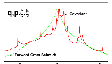
Figure 9: Probability densities for $\lambda^{f}_{22}(t)$ and $\lambda^{c}_{22}(t)$. The logarithmic ordinate scale covers two decades with data from the central two billion out of four billion fourth-order Runge-Kutta timesteps of 0.001 each.

To make it possible for the reader to coordinate our results with those of Wolfe and Samelsonb16 , we write a set of equations which can be solved in order to find the third covariant vector $\delta^{c}_{3}$ as an expansion in the forward-in-time Gram-Schmidt vectors:

$$M^{f}\cdot y=0\ ;\ M^{f}=\left[\begin{array}[]{c c c}\sum(\delta^{f}_{1}\cdot\delta^{b}_{k})(\delta^{b}_{k}\cdot\delta^{f}_{1})&\sum(\delta^{f}_{1}\cdot\delta^{b}_{k})(\delta^{b}_{k}\cdot\delta^{f}_{2})&\sum(\delta^{f}_{1}\cdot\delta^{b}_{k})(\delta^{b}_{k}\cdot\delta^{f}_{3})\\ \sum(\delta^{f}_{2}\cdot\delta^{b}_{k})(\delta^{b}_{k}\cdot\delta^{f}_{1})&\sum(\delta^{f}_{2}\cdot\delta^{b}_{k})(\delta^{b}_{k}\cdot\delta^{f}_{2})&\sum(\delta^{f}_{2}\cdot\delta^{b}_{k})(\delta^{b}_{k}\cdot\delta^{f}_{3})\\ \sum(\delta^{f}_{3}\cdot\delta^{b}_{k})(\delta^{b}_{k}\cdot\delta^{f}_{1})&\sum(\delta^{f}_{3}\cdot\delta^{b}_{k})(\delta^{b}_{k}\cdot\delta^{f}_{2})&\sum(\delta^{f}_{3}\cdot\delta^{b}_{k})(\delta^{b}_{k}\cdot\delta^{f}_{3})\end{array}\right]\ .$$

Here the sums include the two values of $k=1,2$. The numbering system, though arbitrary, is crucial. Forward in time the correspondence of the vectors with the long-time-averaged Lyapunov exponents is

$$\delta^{f}_{1}\rightarrow+0.073\ ;\ \delta^{f}_{2}\rightarrow 0.000\ ;\ \delta^{f}_{3}\rightarrow-0.091\ ;\ \delta^{f}_{4}\rightarrow-0.411\ .$$

Backward in time the ordering is the same with the signs changed:

$$\delta^{b}_{1}\rightarrow-0.073\ ;\ \delta^{b}_{2}\rightarrow 0.000\ ;\ \delta^{b}_{3}\rightarrow+0.091\ ;\ \delta^{b}_{4}\rightarrow+0.411\ .$$

Of course the third covariant vector going forward could equally well be viewed as the second going backward using an expansion in terms of the backward-in-time Gram-Schmidt vectors. This alternative approach results in a smaller matrix without the sum over $k$:

$$M^{b}\cdot y=0\ ;\ M^{b}=\left[\begin{array}[]{c c}(\delta^{b}_{1}\cdot\delta^{f}_{1})(\delta^{f}_{1}\cdot\delta^{b}_{1})&(\delta^{b}_{1}\cdot\delta^{f}_{1})(\delta^{f}_{1}\cdot\delta^{b}_{2})\\ (\delta^{b}_{2}\cdot\delta^{f}_{1})(\delta^{f}_{1}\cdot\delta^{b}_{1})&(\delta^{b}_{2}\cdot\delta^{f}_{1})(\delta^{f}_{1}\cdot\delta^{b}_{2})\end{array}\right]\ .$$

Here the ordering of the Gram-Schmidt vectors follows this same new ordering of the backward vectors:

$$\delta^{b}_{1}\rightarrow+0.411\ ;\ \delta^{b}_{2}\rightarrow+0.091\ ;\ \delta^{b}_{3}\rightarrow 0.000\ ;\ \delta^{b}_{4}\rightarrow-0.073\ .$$

The vectors forward in time follow the same ordering with the signs changed.

Once the ordering of the vectors is correctly negotiated one can find the eight Gram-Schmidt vectors (four in each time direction) and the four covariant vectors (the same in either time direction). For comparison we show the probability densities for the vectors in Figures 10, 11, and 12.

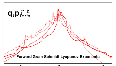
Figure 10: Probability density for the four forward-in-time Lyapunov exponents, $\{\ \lambda^{f}_{ii}(t)\ \}$. Notice that the distribution for the largest of the exponents (widest line) is the same as that for the covariant Lyapunov exponent $\lambda^{c}_{11}(t)$. The logarithmic ordinate scale covers two decades with data from the central two billion out of four billion fourth-order Runge-Kutta timesteps of 0.001 each.

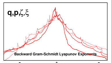
Figure 11: Probability density for the four backward-in-time Lyapunov exponents, $\{\ \lambda^{b}_{ii}(t)\ \}$. Notice that the probability distribution for the most positive of the backward exponents, $\lambda^{b}_{1}=+0.411$ (widest line) matches that for the covariant Lyapunov exponent $\lambda^{c}_{44}(t)$ shown in Figure 12. The logarithmic ordinate scale covers two decades with data from the central two billion out of four billion fourth-order Runge-Kutta timesteps of 0.001 each.

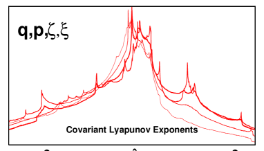
Figure 12: Probability density for the four covariant Lyapunov exponents, $\{\ \lambda^{c}_{ii}(t)\ \}$. The largest and smallest of these exponents match the largest forward and the largest backward of the Gram-Schmidt exponents. The covariant vectors are identical forward or backward in time, with their exponents simply changing sign. The logarithmic ordinate covers two decades with data from the central two billion out of four billion fourth-order Runge-Kutta timesteps of 0.001 each.

V Perspectives

The covariant phase-space vectors, illustrated here for oscillators, are said to have two advantages: [1] they display the time-symmetry of the underlying equations of motion and [2] they provide results which are “norm-independent”. The Gram-Schmidt vectors differ, reflecting the past and steadfastly ignorant of the future. Consider a purely-Hamiltonian situation, the sudden inelastic collision of two rapidly-moving blocks, converting ordered kinetic energy to heat. The Gram-Schmidt vectors turn out to be more localized in the forward direction of time than in the (completely unphysical) reversed direction, where the particle trajectories have been storedb29 . The phase-space directions corresponding to maximum growth and decay (easy to calculate by singular value decomposition of the symmetrized $D$ matrix and relatively smooth in phase space, rather than multifractal) show the same time symmetry as do the covariant vectors. This time symmetry seems unhelpful for describing the irreversibility of this purely-Hamiltonian shockwave process. We like the time asymmetry of the Gram-Schmidt vectors, reflecting as they do the past-based nature of the Second Law of Thermodynamics.

Despite the norm-independence of the Lyapunov vectors it is apparent that “local” (in phase-space or in time) Lyapunov exponents depend on the chosen coordinate system. Even the simple harmonic oscillator considered here shows coordinate-dependent local exponents.

The time symmetry-breaking associated with time-reversible dissipative systems (like the three-dimensional and four-dimensional oscillator models studied here) prevents backward analyses unless trajectories are stored. Lyapunov instability helps attract a repellor state (violating the Second Law) to the Law-abiding strange attractor. Like the overall trajectory, the Gram-Schmidt vectors are themselves unstable to symmetry breaking. A reversed trajectory calculation will not also reverse the Gram-Schmidt vectors unless those vectors too are stored from a forward trajectory. The covariant vectors are the same going forward and backward in time. The symmetry breaking which naturally occurs can only be avoided by repeating a trajectory, making it possible to find the covariant solution.

Despite the double-precision accuracy of Runge-Kutta solutions it is difficult to validate computer programs for dissipative chaotic systems precisely due to their Lyapunov instability. For this reason the squared projections of the offset vectors and the exponent histograms are good choices for validation. The details of specific program results necessarily vary and reflect the fractal nature of the phase-space singularities describing the inevitable past and future bifurcations. The fractal nature of these singular points frustrates any attempt to gain accuracy through mesh refinement. Both the covariant and the Gram-Schmidt exponents share this fractal nature, but differently. The Gram-Schmidt vectors are analogous to passengers’ reactions to a curvy highway while the covariant view is that of a stationary pedestrian observer.

VI Acknowledgments

We thank Mauricio Romero-Bastida and Antonio Politi for useful conversations at a workshop organized by Thomas Gilbert and Dave Sanders, held in Cuernavaca, Mexico earlier this year. Rainer Klages, Pavel Kuptsov, Roger Samelson, Franz Waldner, and Christopher Wolfe generously provided some comments and useful literature references. We specially thank Lakshmi Narayanan for stimulating this work by requesting a Second Edition of our book on Time Reversibility, and Stefano Ruffo, for expediting publication in Communications in Nonlinear Science and Numerical Simulation.

References

- (1) W. G. Hoover, Time Reversibility, Computer Simulation, and Chaos (World Scientific, Singapore, 2001).
- (2) W. G. Hoover, Computational Statistical Mechanics (Elsevier, Amsterdam, 1991, and available free at http://www.williamhoover.info).
- (3) W. G. Hoover and W. T. Ashurst, “Nonequilibrium Molecular Dynamics”, Theoretical Chemistry 1, 1-51 (Academic Press, New York, 1975).
- (4) W. G. Hoover, C. G. Hoover, and J. Petravic, “Simulation of Two- and Three-Dimensional Dense-Fluid Shear Flows via Nonequilibrium Molecular Dynamics: Comparison of Time-and-Space-Averaged Stresses from Homogeneous Doll’s and Sllod Shear Algorithms with Those from Boundary-Driven Shear”, Physical Review E 78, 046701 (2008).
- (5) J. D. Farmer, E. Ott, and J. A. Yorke, “The Dimension of Chaotic Attractors”, Physica 7D, 153-180 (1983).
- (6) S. D. Stoddard and J. Ford, “Numerical Experiments on the Stochastic Behavior of a Lennard-Jones Gas System”, Physical Review A 8, 1504-1512 (1973).
- (7) I. Shimada and T. Nagashima, “A Numerical Approach to Ergodic Problem of Dissipative Dynamical Systems”, Progress of Theoretical Physics 61, 1605-1616 (1979).
- (8) G. Benettin, L. Galgani, and J. M. Strelcyn, “Kolmogorov Entropy and Numerical Experiments”, Physical Review A 14, 2338-2345 (1976).
- (9) E. N. Lorenz, “A Study of the Predictability of a 28-Variable Atmospheric Model”, Tellus 17, 321-333 (1965).
- (10) E. N. Lorenz, “Lyapunov Numbers and the Local Structure of Attractors”, Physica 17D, 279-294 (1985).
-
(11)
Almost all of Edward Norton Lorenz’ publications can be
found on an MIT webpage,
[ http://eapsweb.mit.edu/research/Lorenz/publications/htm ]. - (12) J. P. Eckmann and D. Ruelle, “Ergodic Theory of Chaos and Strange Attractors”, Reviews of Modern Physics 57, 617-656 (1985).
- (13) A. Trevisan and F. Pancotti, “Periodic Orbits, Lyapunov Vectors, and Singular Vectors in the Lorenz System”, Journal of the Atmospheric Sciences 55, 390-398 (1998).
- (14) C. L. Wolfe, “Quantifying Linear Disturbance Growth in Periodic and Aperiodic Systems”, Ph. D. Dissertation written under the Supervision of Roger Samelson, at Oregon State University, 2006.
- (15) F. Ginelli, P. Poggi, A. Turchi, H. Chaté, R. Livi, and A. Politi, “Characterizing Dynamics with Covariant Lyapunov Vectors”, Physical Review Letters 99, 130601 (2007).
- (16) C. L. Wolfe and R. M. Samelson, “An Efficient Method for Recovering Lyapunov Vectors from Singular Vectors”, Tellus 59A, 355-366 (2007).
- (17) M. Romero-Bastida, D. Pazó, J. M. López, and M. A. Rodriguez, “Structure of Characteristic Lyapunov Vectors in Anharmonic Hamiltonian Lattices”, Physical Review E 82, 036205 (2010).
- (18) H. Bosetti, H. A. Posch, Ch. Dellago, and W. G. Hoover, “Time-Reversal Symmetry and Covariant Lyapunov Vectors for the Doubly Thermostated Harmonic Oscillator”, Physical Review E 82, 046218 (2010).
- (19) P. V. Kuptsov and U. Parlitz, “Theory and Computation of Covariant Lyapunov Vectors”, arXiv 1105.5228 (Nonlinear Sciences, Chaotic Dynamics) (26 May 2011).
- (20) W. G. Hoover, C. G. Hoover, and H. A. Posch, “Lyapunov Instability of Pendulums, Chains, and Strings”, Physical Review A 41, 2999-3005 (1990).
- (21) W. G. Hoover and H. A. Posch, “Direct Measurement of Equilibrium and Nonequilibrium Lyapunov Spectra”, Physics Letters A 123, 227-230 (1987).
- (22) I. Goldhirsch, P. L. Sulem, and S. A. Orszag, “Stability and Lyapunov Stability of dynamical Systems: a Differential Approach and a Numerical Method”, Physica 27D, 311-337 (1987).
- (23) W. G. Hoover, Canonical Dynamics: Equilibrium Phase-Space Distributions”, Physical Review A 31, 1695-1697 (1985).
- (24) H. A. Posch, W. G. Hoover, and F. J. Vesely, “Canonical Dynamics of the Nosé Oscillator: Stability, Order, and Chaos”, Physical Review A 33, 4253-4265 (1986).
- (25) Wm. G. Hoover, C. G. Hoover, and F. Grond, “Phase-Space Growth Rates, Local Lyapunov Spectra, and Symmetry Breaking for Time-Reversible Dissipative Oscillators”, Communications in Nonlinear Science and Numerical Simulation 13, 1180-1193 (2008).
- (26) Wm. G. Hoover, C. G. Hoover, and H. A. Posch, “Dynamical Instabilities, Manifolds, and Local Lyapunov Spectra Far From Equilibrium”, Computational Methods in Science and Technology 7, 55-65 (2001).
- (27) Wm. G. Hoover, C. G. Hoover, H. A. Posch, and J. A. Codelli, “The Second Law of Thermodynamics and Multifractal Distribution Functions: Bin Counting, Pair Correlations, and the [Definite Failure of the] Kaplan-Yorke Conjecture”, Communications in Nonlinear Science and Numerical Simulation 12, 214-231 (2005).
- (28) Wm. G. Hoover and B. L. Holian, “Kinetic Moments Method for the Canonical Ensemble Distribution”, Physics Letters A 211, 253-257 (1996).
- (29) Wm. G. Hoover and C. G. Hoover, “Three Lectures: NEMD, SPAM, and Shockwaves”, presented at the Granada Seminar on the Foundations of Nonequilibrium Statistical Physics, 13-17 September, 2010: arXiv:1008.4947.