Dynamical density functional theory for colloidal particles with arbitrary shape

Abstract

Starting from the many-particle Smoluchowski equation, we derive dynamical density functional theory for Brownian particles with an arbitrary shape. Both passive and active (self-propelled) particles are considered. The resulting theory constitutes a microscopic framework to explore the collective dynamical behavior of biaxial particles in nonequilibrium. For spherical and uniaxial particles, earlier derived dynamical density functional theories are recovered as special cases. Our study is motivated by recent experimental progress in preparing colloidal particles with many different biaxial shapes.

I Introduction

In its original form, classical dynamical density functional theory (DDFT) was derived by Marconi and Tarazona MarconiT1999 in 1999 for spherical, i.e., isotropic, colloidal particles. Their derivation started from the Langevin equation for spherical particles Dean1996 that interact via a pair potential. Later, in 2004, DDFT was rederived by Archer and Evans ArcherE2004 from the Smoluchowski equation that corresponds to the Langevin equation for interacting spherical particles. In 2007, DDFT was generalized by Rex, Wensink, and Löwen RexWL2007 to systems of uniaxial anisotropic particles with orientational degrees of freedom. This generalization is based on the Smoluchowski equation for rigid rods Dhont1996 . It made DDFT applicable to the important class of uniaxial liquid crystals.

Nowadays, it is already possible to produce colloidal particles with rather complicated shapes including biaxial particles. Although static classical density functional theory (DFT) has presently available very powerful tools like fundamental measure theory HansenGoosM2009 that allow to consider also such complicated colloidal particles in the context of DFT, the dynamics of these biaxial particles could up to now not be investigated on the basis of DDFT. For these reasons, it is of high importance to push forward the development of DDFT.

In this paper, we present a further generalization of DDFT, which is now also applicable to biaxial particles. This extension of DDFT contains the previous DDFT equations as special cases and does not assume a certain shape for the colloidal particles. Instead, it is derived for arbitrarily shaped colloids. In comparison with the former DDFT approach, this leads to three independent rotational diffusion coefficients instead of only one. Since our new DDFT equation holds also for screw-like particles, it takes even a possible translational-rotational coupling into account. Additionally, we consider a possible self-propulsion mechanism of the particles so that our results are also relevant for the investigation of the collective dynamics of active particles like swarms of swimming microorganisms as, for example, protozoa Ramaswamy2010 .

The paper is organized as follows: after giving a short overview in Sec. II about anisotropic colloidal particle shapes that can already be synthesized, we present our derivation of the extended DDFT equation in Sec. III and discuss special cases that are known from literature. Sec. IV is addressed to possible applications of the DDFT equation. Finally, we give conclusions and mention possible further extensions of DDFT in Sec. V.

II Geometric classification of colloidal particles

Induced by technological advance in the processing of nanomaterials, a large number of differently shaped colloidal particles became synthetizable during the last years. The different shapes of these colloidal particles can be classified by means of their geometric properties. Figure 1 shows a detailed classification of colloidal shapes with respect to symmetry and convexity.

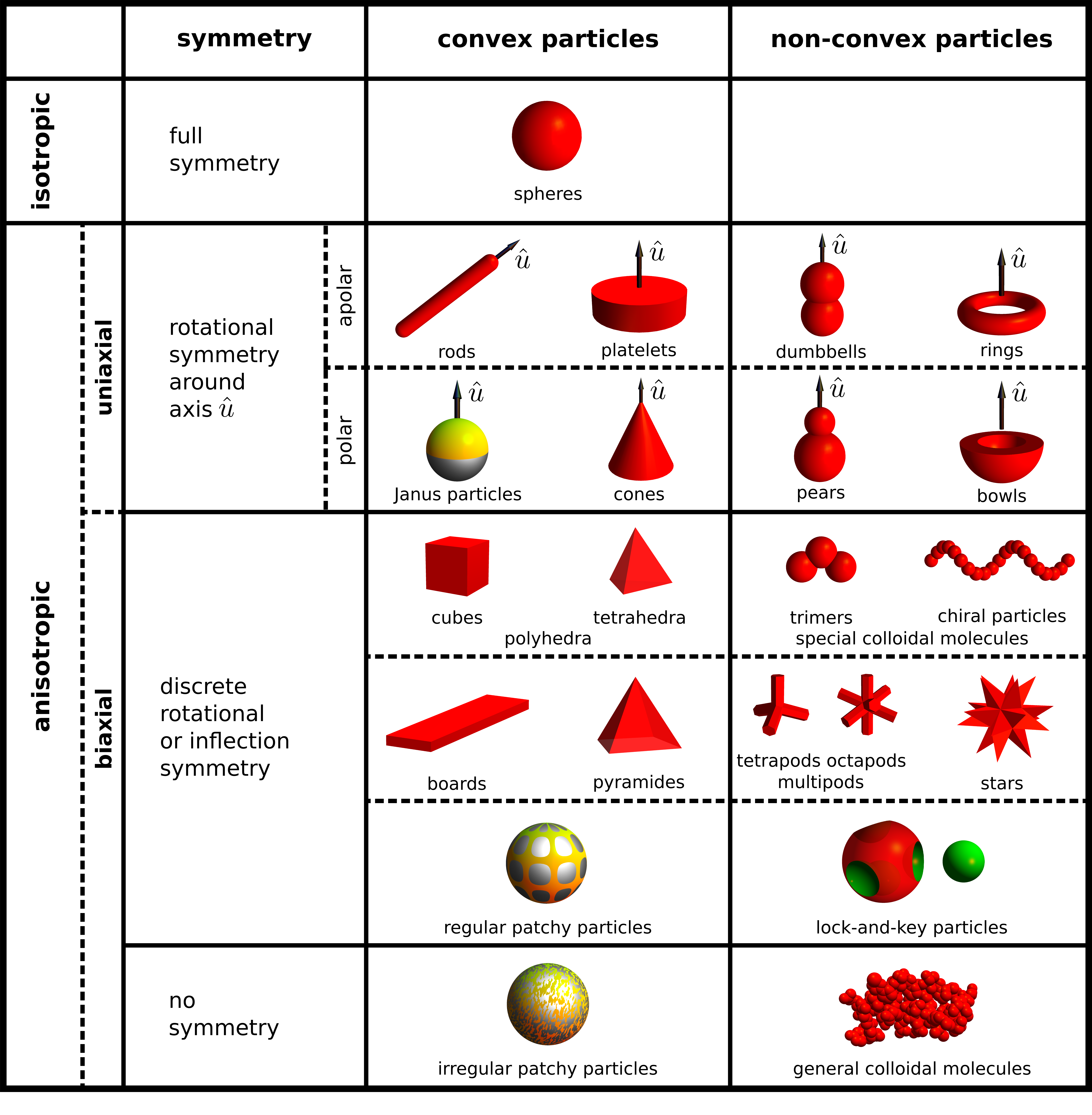
Figure 1: Classification of synthetizable colloidal particles with respect to their shape. Geometrical properties that were used to classify the shapes are symmetry and convexity.

Such a classification is of big importance since colloidal particles may form a huge set of mesotropic phases (mesophases) Chandrasekhar1992 ; Boyd2008K56 that go along with different states of translational and orientational order. The possible states of translational and orientational order depend strongly on the shapes of the particles and a classification of their shapes is therefore also a classification of the possible phases that these particles may evolve.

The most simple and at once full symmetric, i.e., isotropic, shape is the sphere. This is the traditional shape for colloids in theoretical soft matter physics, because it is simple to produce and due to a lack of orientational degrees of freedom relatively simple to describe theoretically. Since spheres possess only translational degrees of freedom, they solely appear in the completely disordered isotropic phase and in the crystalline state HansenMD2006 . The shape of a sphere is globally convex and there is no non-convex analog with full symmetry. All other colloidal particle shapes are anisotropic and either uniaxial or biaxial. The characteristic property of uniaxial particles is a symmetry axis, whose orientation is denoted by the unit vector $\hat{u}$ in the following. These particles have rotational symmetry and possess one orientational degree of freedom in two spatial dimensions and two orientational degrees of freedom in three spatial dimensions. Uniaxial particles are further distinguished into apolar and polar particles. An uniaxial particle is called apolar, if it has head-tail symmetry and polar otherwise. Rod-like particles RoordavDPGvBK2004 ; HanANZLY2006 like spherocylinders, spheroids, and ellipsoids are the most simple anisotropic colloidal particles. They are convex and apolar and of big importance since they may evolve the industrially important nematic phase and serve as excellent model systems for most liquid crystals WeyerichDACK1990 ; TavaresHTdG2009 ; LopezLRPC2010 . A further member of convex and apolar particles are the platelets WierengaLP1998 ; BierHD2005 ; vanderBeekEtAl2006 ; vanderBeekDWVL2008 ; LapointeHMS2010 . They have a similar phase diagram to rod-like particles with a strong affinity to form columnar stacks MouradPVL2010 . Systems of such disk-like particles are realized in nature for example by clay suspensions DijkstraHM1995 ; MourchidDLLL1995 ; DijkstraHM1997 . Examples for non-convex apolar particles are dumbbells (dimers) JohnsonvKvB2005 ; MarechalD2008 ; DemiroersJvKvBI2010 , that are produced by mergence of two spheres of equal size, and rings YanLWLZ2006 ; Thaokar2008 , that can be made by etching from colloidal spheres that are partially embedded in a metal layer. The complement of apolar particles is built by the polar particles, that have no head-tail symmetry. A famous member of this particle class are the Janus particles HongCLG2006 ; HoCSLK2008 ; WaltherM2008 . They are spheres with a different coating at one half of the surface. The original Janus particles had a hydrophilic and a hydrophobic coating. Nowadays, one coating is often reactive like a platinic coating that decomposes hydrogen peroxide catalytically. Such particles are immersed into a hydrogen peroxide solution to realize active particles (micro-swimmers) that are driven by an intrinsic drive FattahLLGWLBA2011 . Cones are a further member of uniaxial polar particles. Carbon nanocones appear naturally in graphite KrishnanDTHLE1997 ; JaszczakRDG2003 ; NalumNaessEHK2009 and do not need to be produced by an elaborate method. By the mergence of two spheres with different diameters, one obtains a pear-like particle KegelBEP2006 ; HoseinJLEL2009 . Pears and also bowls JeongICKX2007 ; MarechalKDID2010 are non-convex particles that are uniaxial and polar. The latter stack into each other and form columnar structures MarechalD2010 .

Particles with less symmetry are biaxial. They are the complement to the uniaxial particles in the class of the anisotropic particles. Biaxial particles have either only discrete symmetries, like inflection symmetry and discrete rotational symmetry, or are completely asymmetric. In both cases, the biaxial particles have three orientational degrees of freedom and a unit vector is no longer sufficient to describe their orientation. Instead, two perpendicular unit vectors or Eulerian angles have to be used DoiE2007 . Due to the additional orientational degree of freedom, the phase diagrams of biaxial colloidal particles are much richer than those for uniaxial particles SircarLW2010 . Convex colloidal particles with discrete rotational or inflection symmetry are, for example, polyhedra like cubes CuestaMR1997 ; MartinezRatonC1999 ; ZhouLXWZZW2006 ; SevonkaevGM2008 and tetrahedra YinW1997 ; HajiAkbariEKZPPMG2009 , boards vandenPolPTWBV2009 , pyramids GuhaKC2004 ; Helseth2005 ; FanTOB2008 , and regular patchy particles ZhangG2004 ; BianchiLTZS2006 ; ChoYKJEYYP2007 ; Sciortino2008 . The latter differ from Janus particles by a patchy coating with a regular, e. g., tetrahedral, arrangement. Non-convex particles with discrete rotational or inflection symmetry include special colloidal molecules that are realized by more than two spheres that are merged in a regular arrangement. Examples for this include trimers LiddellS2003 consisting of three equal spheres and chiral particles ZerroukiBPCB2008 ; WensinkJ2009 consisting of many equal spheres in a helical arrangement, multipod-shaped nanocrystals NewtonW2007 ; DekaMDGBM2010 , stars ZhouLXWZZW2006 ; WuCH2009 , and some lock-and-key particles SacannaICP2010 . Patchy particles may also belong to the class of colloidal particles without any kind of symmetry. This is the case, if the patches are arranged or sized in an irregular way. Irregular patchy particles that are made by coating of spherical particles are always convex. Colloidal molecules of arbitrary shape and size belong on the other hand to the completely asymmetric colloidal particles that are not convex ManoharanEP2003 ; QuillietZRvBI2008 ; SolomonZOSDSBGM2010 ; KraftVvKvBIK2009 .

III Derivation of the DDFT equation

In this derivation, we consider a set of $N$ asymmetric rigid particles in a solvent with dynamic (shear) viscosity $\eta$ and neglect possible additional (for example vibrational) degrees of freedom. We choose the center-of-mass positions $\vec{r}_{i}=(x_{1,i},x_{2,i},x_{3,i})$ and the Eulerian angles $\vec{\varpi}_{i}=(\phi_{i},\theta_{i},\chi_{i})$ with $i=1,\dotsc,N$ to describe their positions and orientations completely. Alternatively, the orientation of the particles could also be described by means of two perpendicular axes CaldereraFW2004 , but for our purposes, the use of Eulerian angles is more appropriate, since they do not involve additional geometric constraints and lead to simpler equations with a more compact notation. The angular velocities $\vec{\omega}_{i}$ that describe the instantaneous rotational motion of the particles can be expressed in terms of the Eulerian angles and their temporal derivatives Schutte1976 . For convenience, we use the convention of Gray and Gubbins GrayG1984 , which is equivalent to the second convention of Schutte Schutte1976 , for the Eulerian angles, since with this convention, the first two Eulerian angles $\phi$ and $\theta$ are identical to the usual azimuthal and polar angles of the spherical coordinate system, respectively. The whole set of particles is then characterized by the positional and orientational ”multivectors” $\vec{r}^{N}=(\vec{r}_{1},\dotsc,\vec{r}_{N})$ and $\vec{\varpi}^{N}=(\vec{\varpi}_{1},\dotsc,\vec{\varpi}_{N})$, respectively. For completeness, we also introduce the abbreviation $\vec{\omega}^{N}=(\vec{\omega}_{1},\dotsc,\vec{\omega}_{N})$, here. The particles are exposed to the (time-dependent) total potential

$$U(\vec{r}^{N}\!,\vec{\varpi}^{N}\!,t)=U_{\mathrm{ext}}(\vec{r}^{N}\!,\vec{\varpi}^{N}\!,t)+U_{\mathrm{int}}(\vec{r}^{N}\!,\vec{\varpi}^{N})\;,$$ (1)

which consists of the external potential

$$U_{\mathrm{ext}}(\vec{r}^{N}\!,\vec{\varpi}^{N}\!,t)=\sum^{N}_{i=1}U_{1}(\vec{r}_{i},\vec{\varpi}_{i},t)$$ (2)

and the total particle interaction potential

$$U_{\mathrm{int}}(\vec{r}^{N}\!,\vec{\varpi}^{N})=\sum^{N}_{\begin{subarray}{c}i,j=1\\ i<j\end{subarray}}U_{2}(\vec{r}_{i},\vec{r}_{j},\vec{\varpi}_{i},\vec{\varpi}_{j})\;.$$ (3)

For both the one-particle interaction potentials $U_{1}(\vec{r}_{i},\vec{\varpi}_{i},t)$ and the two-particle interaction potentials $U_{2}(\vec{r}_{i},\vec{r}_{j},\vec{\varpi}_{i},\vec{\varpi}_{j})$, we assume pairwise additivity. Moreover, we neglect many-particle interaction potentials of higher order than pair interaction potentials. We further introduce the $N$-particle probability distribution function $P(\vec{r}^{N}\!,\vec{\varpi}^{N}\!,t)$ for the probability density to find the $N$ particles at time $t$ with the orientations $\vec{\varpi}^{N}$ at the positions $\vec{r}^{N}$. Successive integration of this function with respect to its positional and orientational degrees of freedom leads to the $n$-particle density ArcherE2004

$$\begin{split}\rho^{(n)}(\vec{r}^{n}\!,\vec{\varpi}^{n}\!,t)&=\frac{N!}{(N-n)!}\int_{\mathcal{V}}\!\!\mathrm{d}V_{n+1}\dotsi\!\!\int_{\mathcal{V}}\!\!\mathrm{d}V_{N}\\ &\times\int_{\mathcal{S}}\!\!\mathrm{d}\Omega_{n+1}\dotsi\!\!\int_{\mathcal{S}}\!\!\mathrm{d}\Omega_{N}P(\vec{r}^{N}\!,\vec{\varpi}^{N}\!,t)\;,\end{split}$$ (4)

where $\mathcal{V}=\mathbb{R}^{3}$ and $\mathcal{S}=[0,2\pi)\times[0,\pi)\times[0,2\pi)$ are the domains for spatial and orientational integration, respectively, $\mathrm{d}V=\mathrm{d}x_{1}\mathrm{d}x_{2}\mathrm{d}x_{3}$ and $\mathrm{d}\Omega=\mathrm{d}\phi\mathrm{d}\theta\sin(\theta)\mathrm{d}\chi$ are the corresponding differentials, and

$$\begin{split}\int_{\mathcal{V}}\!\!\mathrm{d}V&=\int^{\infty}_{0}\!\!\!\!\!\!\mathrm{d}x_{1}\int^{\infty}_{0}\!\!\!\!\!\!\mathrm{d}x_{2}\int^{\infty}_{0}\!\!\!\!\!\!\mathrm{d}x_{3}\;,\\ \int_{\mathcal{S}}\!\!\mathrm{d}\Omega&=\int^{2\pi}_{0}\!\!\!\!\!\!\!\mathrm{d}\phi\int^{\pi}_{0}\!\!\!\!\mathrm{d}\theta\sin(\theta)\int^{2\pi}_{0}\!\!\!\!\!\!\!\mathrm{d}\chi\end{split}$$ (5)

are common abbreviations.

III.1 Smoluchowski equation

We start with the derivation of the Smoluchowski equation for the overdamped Brownian dynamics of $N$ self-propelled biaxial particles. In analogy to the uniaxial passive case (see reference Dhont1996 ), we define the translational gradient operator $\vec{\nabla}_{\vec{r}}=(\partial_{x_{1}},\partial_{x_{2}},\partial_{x_{3}})$ and the rotational gradient operator $\vec{\nabla}_{\vec{\varpi}}=i\hat{\mathrm{L}}$, where $i$ is the imaginary unit and $\hat{\mathrm{L}}=(\mathrm{L}_{x_{1}},\mathrm{L}_{x_{2}},\mathrm{L}_{x_{3}})$ is the angular momentum operator, which can be expressed in terms of the Eulerian angles by Schutte1976

$$\begin{split}i\>\!\mathrm{L}_{x_{1}}&=-\cos(\phi)\cot(\theta)\frac{\partial}{\partial\phi}-\sin(\phi)\frac{\partial}{\partial\theta}\\ &\quad\,+\cos(\phi)\csc(\theta)\frac{\partial}{\partial\chi}\;,\\ i\>\!\mathrm{L}_{x_{2}}&=-\sin(\phi)\cot(\theta)\frac{\partial}{\partial\phi}+\cos(\phi)\frac{\partial}{\partial\theta}\\ &\quad\,+\sin(\phi)\csc(\theta)\frac{\partial}{\partial\chi}\;,\\ i\>\!\mathrm{L}_{x_{3}}&=\frac{\partial}{\partial\phi}\;.\end{split}$$ (6)

We further define the vectors $\vec{\mathfrak{x}}^{N}=(\vec{r}^{N}\!,\vec{\varpi}^{N})$ and $\vec{\mathfrak{v}}^{N}=(\dot{\vec{r}}^{N}\!,\vec{\omega}^{N})$ with $\dot{\vec{r}}^{N}=\mathrm{d}\vec{r}^{N}\!/\mathrm{d}t$ and the operators $\vec{\nabla}_{\vec{r}^{N}}=(\vec{\nabla}_{\vec{r}_{1}},\dotsc,\vec{\nabla}_{\vec{r}_{N}})$, $\vec{\nabla}_{\vec{\varpi}^{N}}=(\vec{\nabla}_{\vec{\varpi}_{1}},\dotsc,\vec{\nabla}_{\vec{\varpi}_{N}})$, and $\vec{\nabla}_{\vec{\mathfrak{x}}^{N}}=(\vec{\nabla}_{\vec{r}^{N}},\vec{\nabla}_{\vec{\varpi}^{N}})$ and write down the continuity equation

$$\frac{\partial}{\partial t}P(\vec{\mathfrak{x}}^{N}\!,t)=-\vec{\nabla}_{\vec{\mathfrak{x}}^{N}}\!\cdot\big{(}\vec{\mathfrak{v}}^{N}P(\vec{\mathfrak{x}}^{N}\!,t)\big{)}\;,$$ (7)

which is a trivial generalization of the continuity equation for passive rods that is described by Dhont in Ref. Dhont1996 . On the Brownian time scale, the total force and torque, acting on an arbitrary particle $i\in\{1,\dotsc,N\}$ are zero. The total force and torque consist of the force $\vec{F}^{(\mathrm{A})}_{i}(\vec{\mathfrak{x}}^{N}\!,t)$ and torque $\vec{T}^{(\mathrm{A})}_{i}(\vec{\mathfrak{x}}^{N}\!,t)$ due to the activity of the self-propelled particle $i$, the hydrodynamic force $\vec{F}^{(\mathrm{H})}_{i}(\vec{\mathfrak{x}}^{N})$ and torque $\vec{T}^{(\mathrm{H})}_{i}(\vec{\mathfrak{x}}^{N})$, the interaction force $\vec{F}^{(\mathrm{I})}_{i}(\vec{\mathfrak{x}}^{N}\!,t)$ and torque $\vec{T}^{(\mathrm{I})}_{i}(\vec{\mathfrak{x}}^{N}\!,t)$ due to the potential $U(\vec{\mathfrak{x}}^{N}\!,t)$, and the Brownian force $\vec{F}^{(\mathrm{Br})}_{i}(\vec{\mathfrak{x}}^{N}\!,t)$ and torque $\vec{T}^{(\mathrm{Br})}_{i}(\vec{\mathfrak{x}}^{N}\!,t)$. With the definition $\vec{X}=(\vec{X}_{1},\dotsc,\vec{X}_{N})$ for $\vec{X}\in\{\vec{F}^{(\,\cdot\,)},\vec{T}^{(\,\cdot\,)},\vec{K}^{(\,\cdot\,)}\}$ and the abbreviations

$$\begin{split}\vec{K}^{(\mathrm{A})}(\vec{\mathfrak{x}}^{N}\!,t)&=(\vec{F}^{(\mathrm{A})}(\vec{\mathfrak{x}}^{N}\!,t),\vec{T}^{(\mathrm{A})}(\vec{\mathfrak{x}}^{N}\!,t))\;,\\ \vec{K}^{(\mathrm{H})}(\vec{\mathfrak{x}}^{N})&=(\vec{F}^{(\mathrm{H})}(\vec{\mathfrak{x}}^{N}),\vec{T}^{(\mathrm{H})}(\vec{\mathfrak{x}}^{N}))\;,\\ \vec{K}^{(\mathrm{I})}(\vec{\mathfrak{x}}^{N}\!,t)&=(\vec{F}^{(\mathrm{I})}(\vec{\mathfrak{x}}^{N}\!,t),\vec{T}^{(\mathrm{I})}(\vec{\mathfrak{x}}^{N}\!,t))\;,\\ \vec{K}^{(\mathrm{Br})}(\vec{\mathfrak{x}}^{N}\!,t)&=(\vec{F}^{(\mathrm{Br})}(\vec{\mathfrak{x}}^{N}\!,t),\vec{T}^{(\mathrm{Br})}(\vec{\mathfrak{x}}^{N}\!,t))\;,\end{split}$$ (8)

this force balance for the $N$ colloidal particles can be expressed by

$$\begin{split}\vec{0}&=\vec{K}^{(\mathrm{A})}(\vec{\mathfrak{x}}^{N}\!,t)+\vec{K}^{(\mathrm{H})}(\vec{\mathfrak{x}}^{N})\\ &\quad+\vec{K}^{(\mathrm{I})}(\vec{\mathfrak{x}}^{N}\!,t)+\vec{K}^{(\mathrm{Br})}(\vec{\mathfrak{x}}^{N}\!,t)\;.\end{split}$$ (9)

The forces and torques resulting from the self-propulsion mechanism of the particles are supposed to be constant with respect to their orientations in the respective body-fixed coordinate systems, but their strengths may vary slowly with time. We denote these forces and torques for a certain particle $i$ in body-fixed Cartesian coordinates by the vector $\vec{K}^{(\mathrm{A})}_{0,i}(\vec{r}_{i},t)$ for $i=1,\dotsc,N$ and the corresponding vector in space-fixed coordinates by

$$\vec{K}^{(\mathrm{A})}_{i}(\vec{r}_{i},\vec{\varpi}_{i},t)=\mathcal{R}^{-1}_{0}(\vec{\varpi}_{i})\vec{K}^{(\mathrm{A})}_{0,i}(\vec{r}_{i},t)$$ (10)

with the diagonal block rotation matrix

$$\mathcal{R}_{0}(\vec{\varpi})=\operatorname{diag}\!\big{(}\mathrm{R}(\vec{\varpi}),\mathrm{R}(\vec{\varpi})\big{)}\;,$$ (11)

where the rotation matrix $\mathrm{R}(\vec{\varpi})$ is defined by

$$\begin{split}\mathrm{R}(\vec{\varpi})&=\mathrm{R}_{3}(\chi)\,\mathrm{R}_{2}(\theta)\,\mathrm{R}_{3}(\phi)\;,\\ \mathrm{R}^{-1}(\vec{\varpi})&=\mathrm{R}^{\mathrm{T}}(\vec{\varpi})=\mathrm{R}_{3}(-\phi)\,\mathrm{R}_{2}(-\theta)\,\mathrm{R}_{3}(-\chi)\end{split}$$ (12)

with the elementary rotation matrices

$$\begin{split}\mathrm{R}_{2}(\varphi)&=\begin{pmatrix}\cos(\varphi)&0&-\sin(\varphi)\\ 0&1&0\\ \sin(\varphi)&0&\cos(\varphi)\end{pmatrix},\\ \mathrm{R}_{3}(\varphi)&=\begin{pmatrix}\cos(\varphi)&\sin(\varphi)&0\\ -\sin(\varphi)&\cos(\varphi)&0\\ 0&0&1\end{pmatrix}.\end{split}$$ (13)

Note that $\vec{K}^{(\mathrm{A})}_{0,i}$ depends most often only on time $t$, but one could also think of swimming microorganisms in a poisoned environment, where $\vec{K}^{(\mathrm{A})}_{0,i}$ also depends on $\vec{r}_{i}$. To simplify the notation in the following, we collect all the $N$ vectors $\vec{K}^{(\mathrm{A})}_{i}(\vec{r}_{i},\vec{\omega}_{i},t)$ in the vector

$$\vec{K}^{(\mathrm{A})}(\vec{\mathfrak{x}}^{N}\!,t)=\mathcal{R}^{-1}(\vec{\varpi}^{N})\vec{K}^{(\mathrm{A})}_{0}(\vec{r}^{N}\!,t)$$ (14)

with the $6N\!\times\!6N$-dimensional rotation matrix

$$\mathcal{R}(\vec{\varpi}^{N})=\operatorname{diag}\!\big{(}\mathcal{R}_{0}(\vec{\varpi}_{1}),\dotsc,\mathcal{R}_{0}(\vec{\varpi}_{N})\big{)}$$ (15)

and the $6N$-dimensional vector

$$\vec{K}^{(\mathrm{A})}_{0}(\vec{r}^{N}\!,t)=\big{(}\vec{K}^{(\mathrm{A})}_{0,1}(\vec{r}_{1},t),\dotsc,\vec{K}^{(\mathrm{A})}_{0,N}(\vec{r}_{N},t)\big{)}\;.$$ (16)

Next, we focus on the hydrodynamic force and torque. They are given by

$$\vec{K}^{(\mathrm{H})}(\vec{\mathfrak{x}}^{N})=-\Upsilon(\vec{\mathfrak{x}}^{N})\cdot\vec{\mathfrak{v}}^{N}$$ (17)

with the microscopic friction matrix Dhont1996

$$\Upsilon(\vec{\mathfrak{x}}^{N})=\begin{pmatrix}\Upsilon^{\mathrm{TT}}(\vec{\mathfrak{x}}^{N})&\Upsilon^{\mathrm{TR}}(\vec{\mathfrak{x}}^{N})\\ \Upsilon^{\mathrm{RT}}(\vec{\mathfrak{x}}^{N})&\Upsilon^{\mathrm{RR}}(\vec{\mathfrak{x}}^{N})\end{pmatrix},$$ (18)

where $\Upsilon^{\mathrm{TT}}(\vec{\mathfrak{x}}^{N})$, $\Upsilon^{\mathrm{TR}}(\vec{\mathfrak{x}}^{N})$, $\Upsilon^{\mathrm{RT}}(\vec{\mathfrak{x}}^{N})$, and $\Upsilon^{\mathrm{RR}}(\vec{\mathfrak{x}}^{N})$ are $3N\!\times\!3N$-dimensional submatrices. The submatrices $\Upsilon^{\mathrm{TT}}(\vec{\mathfrak{x}}^{N})$ and $\Upsilon^{\mathrm{RR}}(\vec{\mathfrak{x}}^{N})$ correspond to pure translational and rotational motion, respectively, while $\Upsilon^{\mathrm{TR}}(\vec{\mathfrak{x}}^{N})$ and $\Upsilon^{\mathrm{RT}}(\vec{\mathfrak{x}}^{N})$ have to be taken into account for particles with a translational-rotational coupling as, for example, screw-like particles. For many other particles like those that are orthotropic, however, $\Upsilon^{\mathrm{TR}}(\vec{\mathfrak{x}}^{N})$ and $\Upsilon^{\mathrm{RT}}(\vec{\mathfrak{x}}^{N})$ vanish. In the following, we neglect hydrodynamic interactions between the colloidal particles. With this assumption, the microscopic friction submatrices simplify to the block diagonal matrices

$$\Upsilon^{\mathrm{TT}}(\vec{\varpi}^{N}) =\operatorname{diag}\!\big{(}\Upsilon^{\mathrm{TT}}_{11}(\vec{\varpi}_{1}),\dotsc,\Upsilon^{\mathrm{TT}}_{NN}(\vec{\varpi}_{N})\big{)}\;,$$ (19)

$$\Upsilon^{\mathrm{TR}}(\vec{\varpi}^{N}) =\operatorname{diag}\!\big{(}\Upsilon^{\mathrm{TR}}_{11}(\vec{\varpi}_{1}),\dotsc,\Upsilon^{\mathrm{TR}}_{NN}(\vec{\varpi}_{N})\big{)}\;,$$ (20)

$$\Upsilon^{\mathrm{RT}}(\vec{\varpi}^{N}) =\operatorname{diag}\!\big{(}\Upsilon^{\mathrm{RT}}_{11}(\vec{\varpi}_{1}),\dotsc,\Upsilon^{\mathrm{RT}}_{NN}(\vec{\varpi}_{N})\big{)}\;,$$ (21)

$$\Upsilon^{\mathrm{RR}}(\vec{\varpi}^{N}) =\operatorname{diag}\!\big{(}\Upsilon^{\mathrm{RR}}_{11}(\vec{\varpi}_{1}),\dotsc,\Upsilon^{\mathrm{RR}}_{NN}(\vec{\varpi}_{N})\big{)}$$ (22)

with the $3\!\times\!3$-dimensional matrices

$$\Upsilon^{\mathrm{TT}}_{ii}(\vec{\varpi}_{i}) =\eta\,\mathrm{R}^{-1}(\vec{\varpi}_{i})\,\mathrm{K}\,\mathrm{R}(\vec{\varpi}_{i})\;,$$ (23)

$$\Upsilon^{\mathrm{TR}}_{ii}(\vec{\varpi}_{i}) =\eta\,\mathrm{R}^{-1}(\vec{\varpi}_{i})\,\mathrm{C}^{\mathrm{(S)T}}\,\mathrm{R}(\vec{\varpi}_{i})\;,$$ (24)

$$\Upsilon^{\mathrm{RT}}_{ii}(\vec{\varpi}_{i}) =\eta\,\mathrm{R}^{-1}(\vec{\varpi}_{i})\,\mathrm{C}^{\mathrm{(S)}}\,\mathrm{R}(\vec{\varpi}_{i})\;,$$ (25)

$$\Upsilon^{\mathrm{RR}}_{ii}(\vec{\varpi}_{i}) =\eta\,\mathrm{R}^{-1}(\vec{\varpi}_{i})\,\Omega^{\mathrm{(S)}}\,\mathrm{R}(\vec{\varpi}_{i})$$ (26)

for $i=1,\dotsc,N$, which are related to the translation tensor $\mathrm{K}$, the coupling tensor $\mathrm{C}^{\mathrm{(S)}}$, its transposed $\mathrm{C}^{\mathrm{(S)T}}$, and the rotation tensor $\Omega^{\mathrm{(S)}}$ HappelB1991 by an orthogonal transformation with the rotation matrix $\mathrm{R}(\vec{\varpi})$. The tensors $\mathrm{K}$, $\mathrm{C}^{\mathrm{(S)}}$, and $\Omega^{\mathrm{(S)}}$ are constant and depend on shape and size of the colloidal particles that are considered, but are independent of the viscosity of the solvent. In addition, $\mathrm{C}^{\mathrm{(S)}}$ and $\Omega^{\mathrm{(S)}}$ depend also on the reference point $\mathrm{S}$, for which the center-of-mass position of the considered colloidal particle should be chosen. In the special case of no hydrodynamic interaction, the inverse of the microscopic friction matrix

$$\Upsilon^{-1}(\vec{\mathfrak{x}}^{N})=\beta\,\mathcal{D}(\vec{\mathfrak{x}}^{N})$$ (27)

with the inverse temperature $\beta=1/(k_{\mathrm{B}}T)$, the Boltzmann constant $k_{\mathrm{B}}$, and the microscopic short-time diffusion matrix

$$\mathcal{D}(\vec{\mathfrak{x}}^{N})=\begin{pmatrix}\mathcal{D}^{\mathrm{TT}}(\vec{\mathfrak{x}}^{N})&\mathcal{D}^{\mathrm{TR}}(\vec{\mathfrak{x}}^{N})\\ \mathcal{D}^{\mathrm{RT}}(\vec{\mathfrak{x}}^{N})&\mathcal{D}^{\mathrm{RR}}(\vec{\mathfrak{x}}^{N})\end{pmatrix},$$ (28)

which we need in the following, has the same structure as the microscopic friction matrix. We further have the equation

$$\vec{K}^{(\mathrm{I})}(\vec{\mathfrak{x}}^{N}\!,t)=-\vec{\nabla}_{\vec{\mathfrak{x}}^{N}}U(\vec{\mathfrak{x}}^{N}\!,t)$$ (29)

for the interaction force and torque. Moreover, the Brownian force and torque $\vec{F}^{(\mathrm{Br})}(\vec{\mathfrak{x}}^{N}\!,t)$ and $\vec{T}^{(\mathrm{Br})}(\vec{\mathfrak{x}}^{N}\!,t)$ can be derived from the equilibrium condition

$$\lim_{t\to\infty}P(\vec{\mathfrak{x}}^{N}\!,t)\propto e^{-\beta U(\vec{\mathfrak{x}}^{N}\!,t)}$$ (30)

when $\vec{K}^{(\mathrm{A})}(\vec{\mathfrak{x}}^{N}\!,t)$ is neglected and the vector $\vec{\mathfrak{v}}^{N}$ in Eq. (7) is expressed in terms of the vectors $\vec{\mathfrak{x}}^{N}$, $\vec{K}^{(\mathrm{I})}(\vec{\mathfrak{x}}^{N}\!,t)$, and $\vec{K}^{(\mathrm{Br})}(\vec{\mathfrak{x}}^{N}\!,t)$ with the help of Eq. (9). This results in

$$\vec{K}^{(\mathrm{Br})}(\vec{\mathfrak{x}}^{N}\!,t)=-\frac{1}{\beta}\vec{\nabla}_{\vec{\mathfrak{x}}^{N}}\ln\!\big{(}P(\vec{\mathfrak{x}}^{N}\!,t)\big{)}\;.$$ (31)

Using Eqs. (9), (17), (29), and (31), the Smoluchowski equation

$$\frac{\partial}{\partial t}P(\vec{\mathfrak{x}}^{N}\!,t)=\hat{\mathcal{L}}\,P(\vec{\mathfrak{x}}^{N}\!,t)$$ (32)

with the Smoluchowski operator

$$\begin{split}\hat{\mathcal{L}}=\vec{\nabla}_{\vec{\mathfrak{x}}^{N}}\!\cdot\Big{(}&\mathcal{D}(\vec{\mathfrak{x}}^{N})\cdot\big{(}\beta\>\!\vec{\nabla}_{\vec{\mathfrak{x}}^{N}}U(\vec{\mathfrak{x}}^{N}\!,t)\\ &-\beta\vec{K}^{(\mathrm{A})}(\vec{\mathfrak{x}}^{N}\!,t)+\vec{\nabla}_{\vec{\mathfrak{x}}^{N}}\big{)}\!\Big{)}\end{split}$$ (33)

follows now directly from the continuity equation (7).

III.2 DDFT equation

Next, we proceed in our derivation by applying the integration operator $N\!\int_{\mathcal{V}}\!\!\mathrm{d}V_{2}\dotsi\!\int_{\mathcal{V}}\!\!\mathrm{d}V_{N}\int_{\mathcal{S}}\!\!\mathrm{d}\Omega_{2}\dotsi\!\int_{\mathcal{S}}\!\!\mathrm{d}\Omega_{N}$ from the left on the Smoluchowski equation (32) and obtain the expression

$$\begin{split}\frac{\partial}{\partial t}\rho(\vec{\mathfrak{x}},t)=\vec{\nabla}_{\vec{\mathfrak{x}}}\cdot\Big{(}\mathcal{D}(\vec{\mathfrak{x}})\cdot\big{(}-\beta\vec{K}_{\mathrm{A}}(\vec{\mathfrak{x}},t)\rho(\vec{\mathfrak{x}},t)&\\ +\vec{\nabla}_{\vec{\mathfrak{x}}}\rho(\vec{\mathfrak{x}},t)+\beta\rho(\vec{\mathfrak{x}},t)\vec{\nabla}_{\vec{\mathfrak{x}}}U_{1}(\vec{\mathfrak{x}},t)-\beta\bar{K}(\vec{\mathfrak{x}},t)&\big{)}\!\Big{)}\end{split}$$ (34)

with the short-time diffusion tensor

$$\mathcal{D}(\vec{\varpi})=\begin{pmatrix}\mathcal{D}^{\mathrm{TT}}_{11}(\vec{\varpi})&\mathcal{D}^{\mathrm{TR}}_{11}(\vec{\varpi})\\ \mathcal{D}^{\mathrm{RT}}_{11}(\vec{\varpi})&\mathcal{D}^{\mathrm{RR}}_{11}(\vec{\varpi})\end{pmatrix}$$ (35)

for the one-particle density $\rho(\vec{\mathfrak{x}},t)\equiv\rho^{(1)}(\vec{\mathfrak{x}},t)$, where we omitted the index $1$ in $\vec{r}_{1}$ and $\vec{\varpi}_{1}$ and used the abbreviations $\vec{\mathfrak{x}}=(\vec{r},\vec{\varpi})$, $\vec{\nabla}_{\vec{\mathfrak{x}}}=(\vec{\nabla}_{\vec{r}},\vec{\nabla}_{\vec{\varpi}})$, $\vec{K}_{\mathrm{A}}(\vec{\mathfrak{x}},t)=\vec{K}^{(\mathrm{A})}_{1}(\vec{\mathfrak{x}},t)$, and $\bar{K}(\vec{\mathfrak{x}},t)=(\bar{F}(\vec{\mathfrak{x}},t),\bar{T}(\vec{\mathfrak{x}},t))$. When we further introduce the integration operator

$$\int_{\mathfrak{G}}\!\!\!\mathrm{d}\mathfrak{V}=\!\int_{\mathcal{V}}\!\!\!\>\!\mathrm{d}V\!\int_{\mathcal{S}}\!\!\!\>\!\mathrm{d}\Omega$$ (36)

with the total integration domain $\mathfrak{G}=\mathcal{V}\times\mathcal{S}$ and the corresponding differential $\mathrm{d}\mathfrak{V}=\mathrm{d}V\mathrm{d}\Omega$, the average force $\bar{F}(\vec{\mathfrak{x}},t)$ and torque $\bar{T}(\vec{\mathfrak{x}},t)$ due to the interaction with other particles in Eq. (34) are given by

$$\bar{K}(\vec{\mathfrak{x}},t)=-\int_{\mathfrak{G}}\!\!\!\mathrm{d}\mathfrak{V}^{\prime}\,\rho^{(2)}(\vec{\mathfrak{x}},\vec{\mathfrak{x}}^{\prime}\!,t)\vec{\nabla}_{\vec{\mathfrak{x}}}U_{2}(\vec{\mathfrak{x}},\vec{\mathfrak{x}}^{\prime})\;.$$ (37)

In equilibrium with $\vec{K}_{\mathrm{A}}(\vec{\mathfrak{x}},t)=\vec{0}$ and $U_{1}=U_{1}(\vec{\mathfrak{x}})$, Eq. (34) reduces to the first equation of the Bogoliubov-Born-Green-Kirkwood-Yvon hierarchy for molecular fluids GrayG1984 :

$$\beta\bar{K}_{0}(\vec{\mathfrak{x}})=\vec{\nabla}_{\vec{\mathfrak{x}}}\rho_{0}(\vec{\mathfrak{x}})+\beta\rho_{0}(\vec{\mathfrak{x}})\vec{\nabla}_{\vec{\mathfrak{x}}}U_{1}(\vec{\mathfrak{x}})\;.$$ (38)

Here, a zero in the index of a function denotes the time-independent equilibrium state of this function. For example, the function $\rho_{0}(\vec{\mathfrak{x}})$ denotes the equilibrium one-particle density field that corresponds to the time-independent prescribed external potential $U_{1}(\vec{\mathfrak{x}})$. On the other hand, we have in equilibrium the relation

$$\begin{split}\vec{\nabla}_{\vec{\mathfrak{x}}}\rho_{0}(\vec{\mathfrak{x}})&+\beta\rho_{0}(\vec{\mathfrak{x}})\vec{\nabla}_{\vec{\mathfrak{x}}}U_{1}(\vec{\mathfrak{x}})\\ &\;\;\;=-\beta\rho_{0}(\vec{\mathfrak{x}})\vec{\nabla}_{\vec{\mathfrak{x}}}\>\!\frac{\operatorname{\delta}\!\mathcal{F}_{\mathrm{exc}}[\rho_{0}(\vec{\mathfrak{x}})]}{\operatorname{\delta}\!\rho_{0}(\vec{\mathfrak{x}})}\end{split}$$ (39)

with the equilibrium Helmholtz excess free-energy functional $\mathcal{F}_{\mathrm{exc}}[\rho_{0}(\vec{\mathfrak{x}})]$. This relation follows with

$$\vec{\nabla}_{\vec{\mathfrak{x}}}\>\!c^{(1)}_{0}(\vec{\mathfrak{x}})=\int_{\mathfrak{G}}\!\!\!\mathrm{d}\mathfrak{V}^{\prime}\,c^{(2)}_{0}(\vec{\mathfrak{x}},\vec{\mathfrak{x}}^{\prime})\vec{\nabla}_{\vec{\mathfrak{x}}^{\prime}}\rho_{0}(\vec{\mathfrak{x}}^{\prime})\;,$$ (40)

where $c^{(n)}_{0}(\vec{\mathfrak{x}}_{1},\dotsc,\vec{\mathfrak{x}}_{n})$ is the $n$-particle direct correlation function in equilibrium, and

$$c^{(1)}_{0}(\vec{\mathfrak{x}})=-\beta\frac{\operatorname{\delta}\!\mathcal{F}_{\mathrm{exc}}[\rho_{0}(\vec{\mathfrak{x}})]}{\operatorname{\delta}\!\rho_{0}(\vec{\mathfrak{x}})}$$ (41)

from the more general form

$$\begin{split}\vec{\nabla}_{\vec{\mathfrak{x}}}\rho_{0}(\vec{\mathfrak{x}})&+\beta\rho_{0}(\vec{\mathfrak{x}})\vec{\nabla}_{\vec{\mathfrak{x}}}U_{1}(\vec{\mathfrak{x}})\\ &\;\;\;=\rho_{0}(\vec{\mathfrak{x}})\int_{\mathfrak{G}}\!\!\!\mathrm{d}\mathfrak{V}^{\prime}\,c^{(2)}_{0}(\vec{\mathfrak{x}},\vec{\mathfrak{x}}^{\prime})\vec{\nabla}_{\vec{\mathfrak{x}}^{\prime}}\rho_{0}(\vec{\mathfrak{x}}^{\prime})\\ \end{split}$$ (42)

of Eqs. (14) and (16) in reference Gubbins1980 . Equations (38) and (39) lead to the equilibrium relation

$$\bar{K}_{0}(\vec{\mathfrak{x}})=-\rho_{0}(\vec{\mathfrak{x}})\vec{\nabla}_{\vec{\mathfrak{x}}}\>\!\frac{\operatorname{\delta}\!\mathcal{F}_{\mathrm{exc}}[\rho_{0}(\vec{\mathfrak{x}})]}{\operatorname{\delta}\!\rho_{0}(\vec{\mathfrak{x}})}\;,$$ (43)

which we use instead of Eq. (37) as closure relation for Eq. (34) in the time-dependent (non-equilibrium) situation. A similar adiabatic approximation was used in the derivations of the DDFT equations for isotropic MarconiT1999 ; ArcherE2004 and uniaxial RexWL2007 colloidal particles. The approximation results in the generalized DDFT equation

$$\begin{split}\frac{\partial\rho(\vec{\mathfrak{x}},t)}{\partial t}=\beta\>\!\vec{\nabla}_{\vec{\mathfrak{x}}}\cdot\biggl{(}\mathcal{D}(\vec{\mathfrak{x}})\cdot\biggl{(}\rho(\vec{\mathfrak{x}},t)\biggl{(}\vec{\nabla}_{\vec{\mathfrak{x}}}\>\!\frac{\operatorname{\delta}\!\mathcal{F}[\rho(\vec{\mathfrak{x}},t)]}{\operatorname{\delta}\!\rho(\vec{\mathfrak{x}},t)}&\\ -\vec{K}_{\mathrm{A}}(\vec{\mathfrak{x}},t)\biggr{)}&\!\biggr{)}\!\biggr{)}\end{split}$$ (44)

for anisotropic colloidal particles with the total equilibrium Helmholtz free-energy functional

$$\mathcal{F}[\rho_{0}(\vec{\mathfrak{x}})]=\mathcal{F}_{\mathrm{id}}[\rho_{0}(\vec{\mathfrak{x}})]+\mathcal{F}_{\mathrm{exc}}[\rho_{0}(\vec{\mathfrak{x}})]+\mathcal{F}_{\mathrm{ext}}[\rho_{0}(\vec{\mathfrak{x}})]$$ (45)

that can be decomposed into the ideal rotator gas part Evans1979

$$\beta\mathcal{F}_{\mathrm{id}}[\rho_{0}(\vec{\mathfrak{x}})]=\int_{\mathfrak{G}}\!\!\!\mathrm{d}\mathfrak{V}\,\rho_{0}(\vec{\mathfrak{x}})\big{(}\ln\!\big{(}\Lambda^{3}\rho_{0}(\vec{\mathfrak{x}})\big{)}-1\big{)}$$ (46)

with the thermal de Broglie wavelength $\Lambda$, the excess free-energy part $\mathcal{F}_{\mathrm{exc}}[\rho_{0}(\vec{\mathfrak{x}})]$, and the contribution Evans1979

$$\mathcal{F}_{\mathrm{ext}}[\rho_{0}(\vec{\mathfrak{x}})]=\int_{\mathfrak{G}}\!\!\!\mathrm{d}\mathfrak{V}\,\rho_{0}(\vec{\mathfrak{x}})U_{1}(\vec{\mathfrak{x}},t)$$ (47)

due to the external potential $U_{1}(\vec{\mathfrak{x}},t)$. The DDFT equation (44) describes the time evolution of the one-particle density for a system of similar anisotropic self-propelled colloidal particles that interact over a pair potential and is the main result of this paper.

IV Special cases and possible applications

There is no translational-rotational coupling in the uniaxial case, which means that $\mathcal{D}^{\mathrm{TR}}(\vec{\mathfrak{x}}^{N})$ and $\mathcal{D}^{\mathrm{RT}}(\vec{\mathfrak{x}}^{N})$ and therefore also $\mathcal{D}^{\mathrm{TR}}_{11}(\vec{\varpi})$ and $\mathcal{D}^{\mathrm{RT}}_{11}(\vec{\varpi})$ vanish in this case. Furthermore, the one-particle density and the free-energy functional do not depend on the angle $\chi$ for uniaxial particles and the translational diffusion tensor can then be written as the matrix $\mathcal{D}^{\mathrm{TT}}(\hat{u})=D_{\parallel}\hat{u}\otimes\hat{u}+D_{\perp}(\mathbf{1}-\hat{u}\otimes\hat{u})$, which obviously only depends on the two independent short-time diffusion coefficients $D_{\parallel}$ and $D_{\perp}$ for diffusion parallel and perpendicular to the orientation of the symmetry axis $\hat{u}=(\sin(\theta)\cos(\phi),\sin(\theta)\sin(\phi),\cos(\theta))$ of the uniaxial particle, respectively, where $\mathbf{1}$ denotes the $3\!\times\!3$-dimensional unit matrix. Also the rotational diffusion matrix becomes quite simple for uniaxial particles. When we use $\mathcal{D}^{\mathrm{RR}}=D_{\mathrm{R}}\mathbf{1}$ with the rotational short-time diffusion coefficient $D_{\mathrm{R}}$ and the considerations above and neglect the self propulsion, we obtain the uniaxial DDFT equation RexWL2007 from our more general DDFT equation (44). From the uniaxial DDFT equation, one can in turn derive the DDFT equation for two spatial dimensions WensinkL2008 as well as the traditional DDFT equation for colloidal particles with spherical symmetry MarconiT1999 ; ArcherE2004 as special cases.

The generalized dynamical density functional theory for passive and active biaxial particles as proposed in Eq. (44) can be numerically solved for a plenty of different problems. For passive particles, one can explore for example: i) the relaxation dynamics towards equilibrium RexWL2007 , ii) the response of the system to time-dependent external potentials HaertelBL2010 , iii) the growth of a thermodynamically stable phase into an unstable phase vanTeeffelenBVL2009 . Interesting effects for self-propelled particles include among others: i) the swarming and clustering behavior of biaxial particles in the bulk and in confinement PeruaniDB2006 ; WensinkL2008 , ii) the combined impact of self-propulsion and external forcing WensinkL2008 , iii) the effect of space- and time-dependent internal forcing Rapaport2007 .

V Conclusions and outlook

In conclusion, starting from the multi-body Smoluchowski equation, we have derived dynamical density functional theory for self-propelled Brownian colloidal particles with arbitrary shape. This study was motivated by recent progress in synthesizing colloidal particles with (almost) arbitrary shape. Our results constitute an important framework for further numerical explorations. This is in particular appealing as since recently an equilibrium density functional is known for arbitrarily shaped hard colloids GrafL1999 ; HansenGoosM2009 ; HansenGoosM2010 which can serve as an input for the dynamical density functional theory. Another possibility to construct a density functional for biaxial particles is a mean-field approximation for repulsive segment potentials RexWL2007 , which works for soft interactions LikosHLL2002 , or a perturbation theory CurtinA1986 ; LikosNL1994 for anisotropic attractions around a spherical reference system. A large number of dynamical problems can then in principle be addressed including the dynamics KirchhoffLK1996 ; Loewen1999 ; MazzaGVKS2010 and relaxation of nematic-like order in confined systems RexWL2007 ; VerhoeffBOvdSL2011 , nematic phases driven by external fields HaertelBL2010 , nucleation kinetics of liquid crystalline phases SchillingF2004 ; ZhangvD2006 ; MillerC2009 ; RavnikZ2009 , and collective behavior of self-propelled particles PeruaniDB2006 ; WensinkL2008 . The results can be checked against Brownian dynamics computer simulations Loewen1994b ; WhiteCH2001 .

Possible extensions for the future are the inclusions of hydrodynamic interactions between the particles which are mediated by the solvent. Dynamical density functional theory of spherical particles was generalized for hydrodynamic interactions RexL2008 ; RexL2009 ; AlmenarR2011 , but this is not yet done for anisotropic particles. Another interesting extension would be towards molecular dynamics which is the appropriate dynamics for molecular liquid crystals. But even for spheres it is much more complicated to formulate a dynamical density functional theory for molecular dynamics MarconiTCM2008 ; Archer2009 ; EspanolL2009 . Finally, the theory can readily be generalized towards binary mixtures PiniTPR2003 .

- (1) U. M. B. Marconi and P. Tarazona, Journal of Chemical Physics 110, 8032 (Apr. 1999)
- (2) D. S. Dean, Journal of Physics A: Mathematical and General 29, L613 (Dec. 1996)
- (3) A. J. Archer and R. Evans, Journal of Chemical Physics 121, 4246 (Sep. 2004)
- (4) M. Rex, H. H. Wensink, and H. Löwen, Physical Review E 76, 021403 (Aug. 2007)
- (5) J. K. G. Dhont, An Introduction to Dynamics of Colloids, 1st ed., Studies in Interface Science, Vol. 2 (Elsevier Science, Amsterdam, 1996) ISBN 0-444-82009-4, p. 642
- (6) H. Hansen-Goos and K. Mecke, Physical Review Letters 102, 018302 (Jan. 2009)
- (7) S. Ramaswamy, Annual Review of Condensed Matter Physics 1, 323 (Aug. 2010)
- (8) S. Chandrasekhar, Liquid crystals, 2nd ed. (Cambridge University Press, Cambridge, 1992) ISBN 0-521-41747-3, p. 480
- (9) R. W. Boyd, “Nonlinear optics,” (Academic Press, Amsterdam, 2008) Chap. 5.6. Nonlinear Optics of Liquid Crystals, pp. 271–276, 3rd ed., ISBN 978-0-12-369470-6
- (10) J. Hansen and I. R. McDonald, Theory of Simple Liquids, 3rd ed. (Elsevier Academic Press, Amsterdam, 2006) ISBN 0-12-370535-5, p. 416
- (11) S. Roorda, T. van Dillen, A. Polman, C. Graf, A. van Blaaderen, and B. J. Kooi, Advanced Materials 16, 235 (Feb. 2004)
- (12) Y. Han, A. M. Alsayed, M. Nobili, J. Zhang, T. C. Lubensky, and A. G. Yodh, Science 314, 626 (Oct. 2006)
- (13) B. Weyerich, B. D’Aguanno, E. Canessa, and R. Klein, Faraday Discussions of the Chemical Society 90, 245 (Jul. 1990)
- (14) J. M. Tavares, B. Holder, and M. M. Telo da Gama, Physical Review E 79, 021505 (Feb. 2009)
- (15) L. López, D. Linares, A. Ramirez-Pastor, and S. Cannas, Journal of Chemical Physics 133, 134706 (Sep. 2010)
- (16) A. M. Wierenga, T. A. J. Lenstra, and A. P. Philipse, Colloids and Surfaces A: Physicochemical and Engineering Aspects 134, 359 (Mar. 1998)
- (17) M. Bier, L. Harnau, and S. Dietrich, Journal of Chemical Physics 123, 114906 (Sep. 2005)
- (18) D. van der Beek, H. Reich, P. van der Schoot, M. Dijkstra, T. Schilling, R. Vink, M. Schmidt, R. van Roij, and H. Lekkerkerker, Physical Review Letters 97, 087801 (Aug. 2006)
- (19) D. van der Beek, P. Davidson, H. H. Wensink, G. J. Vroege, and H. N. W. Lekkerkerker, Physical Review E 77, 031708 (Mar. 2008)
- (20) C. P. Lapointe, S. Hopkins, T. G. Mason, and I. I. Smalyukh, Physical Review Letters 105, 178301 (Oct. 2010)
- (21) M. C. D. Mourad, A. V. Petukhov, G. J. Vroege, and H. N. W. Lekkerkerker, Langmuir 26, 14182 (Aug. 2010)
- (22) M. Dijkstra, J. P. Hansen, and P. A. Madden, Physical Review Letters 75, 2236 (Sep. 1995)
- (23) A. Mourchid, A. Delville, J. Lambard, E. LéColier, and P. Levitz, Langmuir 11, 1942 (Jun. 1995)
- (24) M. Dijkstra, J.-P. Hansen, and P. A. Madden, Physical Review E 55, 3044 (Mar. 1997)
- (25) P. M. Johnson, C. M. van Kats, and A. van Blaaderen, Langmuir 21, 11510 (Oct. 2005)
- (26) M. Marechal and M. Dijkstra, Physical Review E 77, 061405 (Jun. 2008)
- (27) A. Demirörs, P. Johnson, C. van Kats, A. van Blaaderen, and A. Imhof, Langmuir 26, 14466 (Sep. 2010)
- (28) Q. Yan, F. Liu, L. Wang, J. Y. Lee, and X. S. Zhao, Journal of Materials Chemistry 16, 2132 (May 2006)
- (29) R. M. Thaokar, Colloids and Surfaces A: Physicochemical and Engineering Aspects 317, 650 (Mar. 2008)
- (30) L. Hong, A. Cacciuto, E. Luijten, and S. Granick, Nano Letters 6, 2510 (Nov. 2006)
- (31) C. Ho, W. Chen, T. Shie, J. Lin, and C. Kuo, Langmuir 24, 5663 (May 2008)
- (32) A. Walther and A. H. E. Müller, Soft Matter 4, 663 (Apr. 2008)
- (33) Z. Fattah, G. Loget, V. Lapeyre, P. Garrigue, C. Warakulwit, J. Limtrakul, L. Bouffiera, and A. Kuhn, Electrochimica Acta ???, in press (??? 2011)
- (34) A. Krishnan, E. Dujardin, M. M. J. Treacy, J. Hugdahl, S. Lynum, and T. W. Ebbesen, Nature 388, 451 (Jul. 1997)
- (35) J. A. Jaszczak, G. W. Robinson, S. Dimovski, and Y. Gogotsi, Carbon 41, 2085 (Aug. 2003)
- (36) S. Nalum Naess, A. Elgsaeter, G. Helgesen, and K. D. Knudsen, Science and Technology of Advanced Materials 10, 065002 (Dec. 2009)
- (37) W. K. Kegel, D. Breed, M. Elsesser, and D. J. Pine, Langmuir 22, 7135 (Jul. 2006)
- (38) I. D. Hosein, B. S. John, S. H. Lee, F. A. Escobedo, and C. M. Liddell, Journal of Materials Chemistry 19, 344 (Jan. 2009)
- (39) U. Jeong, S. H. Im, P. H. C. Camargo, J. H. Kim, and Y. Xia, Langmuir 23, 10968 (Oct. 2007)
- (40) M. Marechal, R. J. Kortschot, A. F. Demirörs, A. Imhof, and M. Dijkstra, Nano Letters 10, 1907 (Apr. 2010)
- (41) M. Marechal and M. Dijkstra, Physical Review E 82, 031405 (Sep. 2010)
- (42) M. Doi and S. F. Edwards, The Theory of Polymer Dynamics, 1st ed., International Series of Monographs on Physics, Vol. 73 (Oxford University Press, Oxford, 2007) ISBN 978-0-19-852033-7, p. 391
- (43) S. Sircar, J. Li, and Q. Wang, Communications in Mathematical Sciences 8, 697 (Sep. 2010)
- (44) J. A. Cuesta and Y. Martínez-Ratón, Journal of Chemical Physics 107, 6379 (Oct. 1997)
- (45) Y. Martínez-Ratón and J. A. Cuesta, Journal of Chemical Physics 111, 317 (Jul. 1999)
- (46) G. Zhou, M. Lü, Z. Xiu, S. Wang, H. Zhang, Y. Zhou, and S. Wang, Journal of Physical Chemistry B 110, 6543 (Feb. 2006)
- (47) I. Sevonkaev, D. V. Goia, and E. Matijević, Journal of Colloid and Interface Science 317, 130 (Jan. 2008)
- (48) J. S. Yin and Z. L. Wang, Physical Review Letters 79, 2570 (Sep. 1997)
- (49) A. Haji-Akbari, M. Engel, A. S. Keys, X. Zheng, R. G. Petschek, P. Palffy-Muhoray, and S. C. Glotzer, Nature 462, 773 (Dec. 2009)
- (50) E. van den Pol, A. V. Petukhov, D. M. E. Thies-Weesie, D. V. Byelov, and G. J. Vroege, Physical Review Letters 103, 258301 (Dec. 2009)
- (51) P. Guha, S. Kar, and S. Chaudhuri, Applied Physics Letters 85, 3851 (Oct. 2004)
- (52) L. E. Helseth, Langmuir 21, 7276 (Aug. 2005)
- (53) D. Fan, P. J. Thomas, and P. O’Brien, Journal of the American Chemical Society 130, 10892 (Jul. 2008)
- (54) Z. Zhang and S. C. Glotzer, Nano Letters 4, 1407 (Jul. 2004)
- (55) E. Bianchi, J. Largo, P. Tartaglia, E. Zaccarelli, and F. Sciortino, Physical Review Letters 97, 168301 (Oct. 2006)
- (56) Y. Cho, G. Yi, S. Kim, S. Jeon, M. Elsesser, H. Yu, S. Yang, and D. J. Pine, Chemistry of Materials 19, 3183 (May 2007)
- (57) F. Sciortino, European Physical Journal B 64, 505 (Aug. 2008)
- (58) C. M. Liddell and C. J. Summers, Advanced Materials 15, 1715 (Oct. 2003)
- (59) D. Zerrouki, J. Baudry, D. Pine, P. Chaikin, and J. Bibette, Nature 455, 380 (Sep. 2008)
- (60) H. H. Wensink and G. Jackson, Journal of Chemical Physics 130, 234911 (Jun. 2009)
- (61) M. C. Newton and P. A. Warburton, Materials Today 10, 50 (May 2007)
- (62) S. Deka, K. Miszta, D. Dorfs, A. Genovese, G. Bertoni, and L. Manna, Nano Letters 10, 3770 (Sep. 2010)
- (63) H.-L. Wu, C.-H. Chen, and M. H. Huang, Chemistry of Materials 21, 110 (Jan. 2009)
- (64) S. Sacanna, W. T. M. Irvine, P. M. Chaikin, and D. J. Pine, Nature 464, 575 (Mar. 2010)
- (65) V. N. Manoharan, M. T. Elsesser, and D. J. Pine, Science 301, 483 (Jul. 2003)
- (66) C. Quilliet, C. Zoldesi, C. Riera, A. van Blaaderen, and A. Imhof, European Physical Journal E 27, 13 (Sep. 2008)
- (67) M. J. Solomon, R. Zeitoun, D. Ortiz, K. E. Sung, D. Deng, A. Shah, M. A. Burns, S. C. Glotzer, and J. M. Millunchick, Macromolecular Rapid Communications 31, 196 (Jan. 2010)
- (68) D. J. Kraft, W. S. Vlug, C. M. van Kats, A. van Blaaderen, A. Imhof, and W. K. Kegel, Journal of the American Chemical Society 131, 1182 (Jan. 2009)
- (69) M. C. Calderera, M. G. Forest, and Q. Wang, Journal of Non-Newtonian Fluid Mechanics 120, 69 (2004)
- (70) C. J. H. Schutte, The Theory of Molecular Spectroscopy: The Quantum Mechanics and Group Theory of Vibrating and Rotating Molecules, 1st ed., The Theory of Molecular Spectroscopy, Vol. 1 (North-Holland Publishing Company, Amsterdam, 1976) ISBN 0-7204-0291-3, p. 512
- (71) C. G. Gray and K. E. Gubbins, Theory of Molecular Fluids: Fundamentals, 1st ed., International Series of Monographs on Chemistry 9, Vol. 1 (Oxford University Press, Oxford, 1984) ISBN 0-19-855602-0, p. 626
- (72) J. Happel and H. Brenner, Low Reynolds number hydrodynamics: with special applications to particulate media, 2nd ed., Mechanics of fluids and transport processes, Vol. 1 (Kluwer Academic Publishers, Dordrecht, 1991) ISBN 90-247-2877-0, p. 553
- (73) The reason for us to write instead of in Eqs. (33\@@italiccorr) and (34\@@italiccorr) is that one could in principle also describe systems with a space-dependent short-time diffusion tensor. This is especially relevant for fluids with a space-dependent viscosity.
- (74) K. E. Gubbins, Chemical Physics Letters 76, 329 (Dec. 1980)
- (75) R. Evans, Advances in Physics 28, 143 (Mar. 1979)
- (76) H. H. Wensink and H. Löwen, Physical Review E 78, 031409 (Sep. 2008)
- (77) A. Härtel, R. Blaak, and H. Löwen, Physical Review E 81, 051703 (May 2010)
- (78) S. van Teeffelen, R. Backofen, A. Voigt, and H. Löwen, Physical Review E 79, 051404 (May 2009)
- (79) F. Peruani, A. Deutsch, and M. Bär, Physical Review E 74, 030904 (Sep. 2006)
- (80) D. C. Rapaport, Physical Review Letters 99, 238101 (Dec. 2007)
- (81) H. Graf and H. Löwen, Journal of Physics: Condensed Matter 11, 1435 (Feb. 1999)
- (82) H. Hansen-Goos and K. Mecke, Journal of Physics: Condensed Matter 22, 364107 (Aug. 2010)
- (83) C. N. Likos, N. Hoffmann, H. Löwen, and A. A. Louis, Journal of Physics: Condensed Matter 14, 7681 (Aug. 2002)
- (84) W. A. Curtin and N. W. Ashcroft, Physical Review Letters 56, 2775 (Jun. 1986)
- (85) C. N. Likos, Z. T. Nemeth, and H. Löwen, Journal of Physics: Condensed Matter 6, 10965 (Dec. 1994)
- (86) T. Kirchhoff, H. Löwen, and R. Klein, Physical Review E 53, 5011 (May 1996)
- (87) H. Löwen, Physical Review E 59, 1989 (Feb. 1999)
- (88) M. G. Mazza, M. Greschek, R. Valiullin, J. Kärger, and M. Schoen, Physical Review Letters 105, 227802 (2010 2010)
- (89) A. A. Verhoeff, I. A. Bakelaar, R. H. J. Otten, P. van der Schoot, and H. N. W. Lekkerkerker, Langmuir 27, 116 (Jan. 2011)
- (90) T. Schilling and D. Frenkel, Journal of Physics: Condensed Matter 16, 2029 (May 2004)
- (91) Z. X. Zhang and J. S. van Duijneveldt, Journal of Chemical Physics 124, 154910 (Apr. 2006)
- (92) W. L. Miller and A. Cacciuto, Physical Review E 80, 021404 (Aug. 2009)
- (93) M. Ravnik and S. Z̆umer, Soft Matter 5, 269 (Jan. 2009)
- (94) H. Löwen, Physical Review E 50, 1232 (Aug. 1994)
- (95) T. O. White, G. Ciccotti, and J. Hansen, Molecular Physics 99, 2023 (Dec. 2001)
- (96) M. Rex and H. Löwen, Physical Review Letters 101, 148302 (Oct. 2008)
- (97) M. Rex and H. Löwen, European Physical Journal E 28, 139 (Feb. 2009)
- (98) L. Almenar and M. Rauscher, Journal of Physics: Condensed Matter 23, 184115 (Apr. 2011)
- (99) U. M. B. Marconi, P. Tarazona, F. Cecconi, and S. Melchionna, Journal of Physics: Condensed Matter 20, 4233 (Dec. 2008)
- (100) A. J. Archer, Journal of Chemical Physics 130, 014509 (Jan. 2009)
- (101) P. Español and H. Löwen, Journal of Chemical Physics 131, 244101 (Dec. 2009)
- (102) D. Pini, M. Tau, A. Parola, and L. Reatto, Physical Review E 67, 046116 (Apr. 2003)