Critical Behavior of AC Antiferromagnetic and Ferromagnetic Susceptibilities of a Spin-$1/2$ Metamagnetic Ising System

Gul Gulpinar a corresponding author. gul.gulpinar@deu.edu.tr Erol Vatansever a Dokuz Eylul University, Department of Physics, 35160-Buca, Izmir, Turkey
Abstract

In this study, the temperature variations of the equilibrium and the non-equilibrium antiferromagnetic and ferromagnetic susceptibilities of a metamagnetic system are examined near the critical point. The kinetic equations describing the time dependencies of the total and staggered magnetizations are derived by utilizing linear response theory. In order to obtain dynamic magnetic relaxation behavior of the system, the stationary solutions of the kinetic equations in existence of sinusoidal staggered and physical external magnetic fields are performed. In addition, the static and dynamical mean field critical exponents are calculated in order to formulate the critical behavior of antiferromagnetic and ferromagnetic magnetic response of a metamagnetic system. Finally, a comparison of the findings of this study with previous theoretical and experimental studies is represented and it is shown that a good agreement is found with our results.

keywords:
Irreversible Thermodynamics, Staggered Magnetic Susceptibility, Direct Magnetic Susceptibility, Metamagnetism, Mean Field Dynamic Critical Exponents.
††journal: Journal of Magnetism and Magnetic Materials

,

1 Introduction

Investigation of the AC or dynamic susceptibilities are the most preferred techniques to study Magnetic relaxation (MR) which is related to magnetic hysteresis and present in all stages of the development of ordered phase is an important approach to probe magnetic systems. They are obtained from the dynamic response of the system to time-dependent magnetic field and now commonly used to investigate the magnetic properties of high-$T_{c}$ systems [1], cobalt-based alloys [2] , nanoparticles [3], spin glasses [4], molecule-based magnets [5], and magnetic fluids [6]. Theoretical investigation of dynamic magnetic response of the Ising models has been an subject of interest for quite a long time: In 1966, Barry has studied spin-$1/2$ Ising model by a method combining statistical theory of phase transitions and irreversible thermodynamics [7]. Using the same method, Barry and Harrington has focused on the theory of relaxation phenomena in an antiferromagnet [8]. In addition, they obtained the temperature and frequency dependencies of the magnetic absorption and dispersion factor in the neighborhood of the critical temperature. On the other hand, Suzuki and Kubo has obtained the time dependent susceptibility of the kinetic Ising model [9]. Acharyya and Chakrabarti presented the real and imaginary parts of magnetic susceptibility near the order disorder transition point of a spin-$1/2$ Ising system in the presence of a periodically varying external field by using Monte-Carlo simulations [10]. On the other hand, The dynamic magnetic response of the materials and the development of methods for its modification are important for their potential applications: Cores made of cobalt-based alloys in low signal detectors of gravitational physics contribute as a noise source with a spectral density proportional to the ac susceptibility of the alloy [2]; MR effects in nanocomposite particles are used in design of magneto-optical devices [3]; the superposition principle for the imaginary part of complex magnetic susceptibility of composite magnetic fluids is crucial for the design of absorbers and microwave attenuators which are based on ferromagnetic resonance absorption of the electromagnetic field [6].

Recently, Erdem investigated the magnetic relaxation in a spin-$1$ Ising model near the second-order phase transition point. In this study, time derivatives of the dipolar and quadrupolar order parameters are treated as fluxes conjugate to their appropriate generalized forces in the sense of irreversible thermodynamics [11]. In addition, Erdem has obtained the frequency dependence of the complex susceptibility for the same system [12]. Though the MR has been subject of many theoretical and experimental investigations mentioned above, there has been no study to investigate the behavior of ac susceptibility in the metamagnetic Ising system.

Metamagnets, systems in which antiferromagnetic and ferromagnetic interactions exist simultaneously, are of great interest because it is possible to induce novel kinds of critical behavior by forcing competition between these couplings, in particular by applying a magnetic field [13]. The metamagnetic model that has in-plane ferromagnetic coupling and antiferromagnetic coupling between adjacent planes, and the next nearest neighbor $(nnn)$ spin-$1/2$ Ising model with antiferromagnetic nearest-neighbour $(nn)$ and ferromagnetic nnn interactions are the theoretical Hamiltonian models showing a similar kind of behavior. These models have been investigated by Monte-Carlo simulations [14], as well as High-temperature series expansion calculations [15].

$FeBr_{2}$ and $FeCl_{2}$ are typical Ising type metamagnets [13]. In these structures, in the antiferromagnetic phase when the iron ions in the triangular layers order ferromagnetically, a layer with a negative sign follows a layer with a positive sign. Due to this fact, the external field acts differently on the oppositely oriented layers which leads to different ordered states and associates a sequence of phase transitions as a function of these two interaction strengths. A Monte-Carlo simulation has been performed on a realistic model of $FeCl_{2}$ under an external magnetic field [16], in addition this typical metamagnet has also been treated by a high-density expansion method on a two-sublattice collinear Heisenberg Ising model with three- and four-ion anisotropy [17, 18]. Dynamic properties of these systems have been investigated by using three-spin flip dynamics [19], Kawasaki dynamics [20], Glauber dynamics [21], and dynamic Monte Carlo renormalization group method [22]. In our recent works we have calculated the kinetic phase diagrams of the system under an oscillating field [23, 24]. Moreover, we have presented an investigation of the relaxation dynamics of iron group dihalides and studied the field and temperature dependence of the relaxation times via the phenomenological kinetic coefficients [25]. Recently Gulpinar and Karaaslan performed an investigation of the relaxation times with taking in account the interference between the relaxation processes of antiferromagnetic and ferromagnetic order parameters [26].

The purpose of this paper is to study the dynamical magnetic response properties of the spin-$1/2$ Ising model in the presence of oscillating external magnetic field. On the other hand, to the best our knowledge there is no study in the literature which represents the mean field calculations for the static staggered and direct susceptibilities of a metamagnetic Ising system. Since then we have given the derivation of the static magnetic response functions and their temperature variations near the critical point in Sec.2. Then, in Sec.3 we derived the temperature and frequency dependent dynamic staggered and direct susceptibilities by a similar method previously used to study relaxation dynamics and sound propagation [27] and investigate the behaviors of magnetic dispersion and absorption factors near the second order phase transition temperature. The method used in this paper provides information about the dynamical critical properties based on the phenomenological kinetic coefficients of the phenomenological rate equations, which governs the magnetization relaxation, is due to an ”ad hoc” spin-lattice coupling.

2 Derivation of Static Staggered Magnetic and Magnetic Susceptibilities of Spin-1/2 Metamagnetic Ising Model

In order to obtain static staggered magnetic susceptibility one should introduce a staggered external field $B_{s}$ to the system [28] whereas magnetic susceptibility is the response of the total magnetization to a physical external field $B$. Since then one should add two different magnetic fields to the Hamiltonian of the spin-1/2 Metamagnetic Ising Model:

$$\displaystyle\hat{H}=\displaystyle-\mathcal{J}\sum_{nn}S_{i}S_{j}+\mathcal{J}^{{}^{\prime}}\sum_{nnn}S_{i}S_{j}-\mu B\sum_{i=1}^{N}S_{i}-\mu B_{s}\left(\sum_{1}S_{i}-\sum_{2}S_{j}\right).$$ (1)

$\mathcal{J},\mathcal{J}^{{}^{\prime}},\mu,B$ and $B_{s}$ are ferromagnetic and antiferromagnetic exchange interaction constants, spin magnetic moment, external magnetic field and external staggered field respectively. By making use of mean field approximation free energy of the system can be obtained as following:

$$\begin{array}[]{lcl}G(m_{t},m_{s},T,B,B_{s})&=&\frac{1}{2}JN(m_{t}^{2}-m_{s}^{2})-\frac{1}{2}J^{{}^{\prime}}N(m_{s}^{2}+m_{t}^{2})\\ &&-\frac{1}{4}k_{B}TN(4\ln(2)-(1+m_{s}+m_{t})\ln(1+m_{s}+m{t})\\ &&-(1-m_{s}-m_{t})\ln(1-m_{s}-m_{t})-(1+m_{t}-m_{s})\\ &&\ln(1+m_{t}-m_{s})-(1-m_{t}+m_{s})\ln(1-m_{t}+m_{s}))\\ &&-Ng\mu_{B}Bm_{t}-Ng\mu_{B}m_{s}B_{s},\end{array}$$ (2)

where $k_{B},g,\mu_{B},N$ are the Boltzmann’s constant, the spin factor, the Bohr magneton and the total number of metamagnetic Ising spins respectively. For a simple cubic lattice in which intralayer interactions are ferromagnetic and interlayer interactions are antiferromagnetic $z=2$ and $z^{{}^{\prime}}=4$. The equilibrium conditions, (βˆ‚Gβˆ‚mt=0,βˆ‚Gβˆ‚ms=0)formulae-sequence𝐺subscriptπ‘šπ‘‘0𝐺subscriptπ‘šπ‘ 0\left(\displaystyle\frac{\partial G}{\partial m_{t}}=0,\frac{\partial G}{\partial m_{s}}=0\right) result in the following transcendental equations:

mt=sinh⁑(2​Bβˆ’mt​fkB​T)cosh⁑(2​Bβˆ’mt​fkB​T)+cosh⁑(2​Bs+ms​tkB​T),ms=sinh⁑(2​Bs+ms​tkB​T)cosh⁑(2​Bβˆ’mt​fkB​T)+cosh⁑(2​Bs+ms​tkB​T).subscriptπ‘šπ‘‘2𝐡subscriptπ‘šπ‘‘π‘“subscriptπ‘˜π΅π‘‡2𝐡subscriptπ‘šπ‘‘π‘“subscriptπ‘˜π΅π‘‡2subscript𝐡𝑠subscriptπ‘šπ‘ π‘‘subscriptπ‘˜π΅π‘‡missing-subexpressionmissing-subexpressionmissing-subexpressionsubscriptπ‘šπ‘ 2subscript𝐡𝑠subscriptπ‘šπ‘ π‘‘subscriptπ‘˜π΅π‘‡2𝐡subscriptπ‘šπ‘‘π‘“subscriptπ‘˜π΅π‘‡2subscript𝐡𝑠subscriptπ‘šπ‘ π‘‘subscriptπ‘˜π΅π‘‡\begin{array}[]{lcl}\displaystyle m_{t}&=&\displaystyle\frac{\sinh(2\frac{B-m_{t}f}{k_{B}T})}{\cosh(2\frac{B-m_{t}f}{k_{B}T})+\cosh(2\frac{B_{s}+m_{s}t}{k_{B}T})},\\ \\ \displaystyle m_{s}&=&\displaystyle\frac{\sinh(2\frac{B_{s}+m_{s}t}{k_{B}T})}{\cosh(2\frac{B-m_{t}f}{k_{B}T})+\cosh(2\frac{B_{s}+m_{s}t}{k_{B}T})}.\end{array} (3)

Here, $f=J-J^{\prime}$ and $t=J+J^{\prime}$. These equations may be solved without difficulty by an iterative procedure, i.e. Newton Raphson method. The equilibrium solutions should correspond to extremum of the free energy so that one has to determine the solution that minimizes $G$ [28]. Since the solution of these equations are discussed in Ref. [25] extensively, we shall only give a brief summary here as follows: Topology of the metamagnetic Ising model phase diagram depends on the value of the ratio of the exchange interactions ($\eta=\frac{J}{J^{\prime}}$): (i)If $\eta>0.6$, the transitions between the anti-ferromagnetic and paramagnetic phases are of first order at low temperatures and strong fields while it is of second order at higher temperatures. The two types of transitions are connected by a tricritical point. (ii) For $0<\eta<0.6$, the tricritical point decomposes into a critical end point (CEP) and a double cricital end point (DCP) with a line of first order transitions in between, separating two anti-ferromagnetic phases [28, 29], see Fig.1(b)-(c) in Ref.[25]. By definition staggered magnetic susceptibility is,

Ο‡ss​t​a​t​i​c=limBsβ†’0βˆ‚msβˆ‚Bs,(B=B0)subscriptπœ’subscriptπ‘ π‘ π‘‘π‘Žπ‘‘π‘–π‘subscriptβ†’subscript𝐡𝑠0subscriptπ‘šπ‘ subscript𝐡𝑠𝐡subscript𝐡0\chi_{s_{static}}=\lim\limits_{B_{s}\rightarrow 0}\frac{\partial m_{s}}{\partial B_{s}},\quad\quad(B=B_{0}) (4)

and total (direct) magnetic susceptibility can be expressed as,

Ο‡ts​t​a​t​i​c=limBsβ†’0βˆ‚mtβˆ‚B(B=B0).subscriptπœ’subscriptπ‘‘π‘ π‘‘π‘Žπ‘‘π‘–π‘subscriptβ†’subscript𝐡𝑠0subscriptπ‘šπ‘‘π΅π΅subscript𝐡0\chi_{t_{static}}=\lim\limits_{B_{s}\rightarrow 0}\frac{\partial m_{t}}{\partial B}\quad\quad(B=B_{0}). (5)

If one uses the equations of state given in Eq.(3), the static staggered magnetic and magnetic susceptibilities can be found as,

Ο‡ss​t​a​t​i​c=limBsβ†’0(a21​c1βˆ’a11​c2a22​a11βˆ’a21​a12),Ο‡ts​t​a​t​i​c=limBsβ†’0(b22​d1βˆ’b12​d2b11​b22βˆ’b12​b21).subscriptπœ’subscriptπ‘ π‘ π‘‘π‘Žπ‘‘π‘–π‘subscriptβ†’subscript𝐡𝑠0subscriptπ‘Ž21subscript𝑐1subscriptπ‘Ž11subscript𝑐2subscriptπ‘Ž22subscriptπ‘Ž11subscriptπ‘Ž21subscriptπ‘Ž12missing-subexpressionmissing-subexpressionmissing-subexpressionsubscriptπœ’subscriptπ‘‘π‘ π‘‘π‘Žπ‘‘π‘–π‘subscriptβ†’subscript𝐡𝑠0subscript𝑏22subscript𝑑1subscript𝑏12subscript𝑑2subscript𝑏11subscript𝑏22subscript𝑏12subscript𝑏21\begin{array}[]{lcl}\chi_{s_{static}}&=&\displaystyle\lim\limits_{B_{s}\rightarrow 0}\left(\frac{a_{21}c_{1}-a_{11}c_{2}}{a_{22}a_{11}-a_{21}a_{12}}\right),\\ \\ \chi_{t_{static}}&=&\displaystyle\lim\limits_{B_{s}\rightarrow 0}\left(\frac{b_{22}d_{1}-b_{12}d_{2}}{b_{11}b_{22}-b_{12}b_{21}}\right).\end{array} (6)

Where, $a_{11},a_{12},a_{21},a_{22},c_{1},c_{2}$, and $b_{11},b_{12},b_{21},b_{22},d_{1},d_{2}$ are given in Appendix-A.
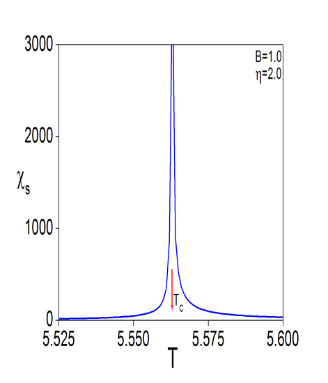
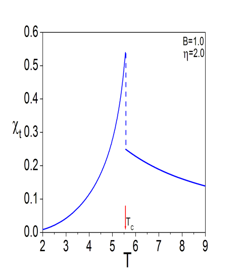
Fig.1(a)-(b) represents the critical behavior of static staggered magnetic susceptibility (Ο‡ssubscriptπœ’π‘ \chi_{s}) and direct magnetic susceptibility. The arrows illustrate the phase transition temperature $T_{C}(B)$ for $B=1.0$. The staggered magnetic susceptibility (Ο‡ssubscriptπœ’π‘ \chi_{s}) increases rapidly with increasing temperature and diverges as the temperature approaches to the second order phase transition point on either side, as seen in Fig.1(a). On the other hand, the magnetic susceptibility $(\chi_{t})$ also increases rapidly when the temperature is raised but makes finite jump discontinuity at the second order phase transition temperature, which is illustrated in Fig.1(b). These findings are in accordance with the results given in Refs.[30, 31] obtained within effective field approximation for an diluted metamagnetic Ising Model. We should also note that Barry and Harrington have given an detailed analysis for the static total susceptibility of an antiferromagnetic Ising system in the Bethe-Takagi approximation which has the same result of the constant-coupling approximation of Kasteleyn and Van Kranendock applied to Ising antiferromagnetism [32]. In both studies an finite jump discontinuity is observed at the critical points which is in accordance with our results. On the other hand, a infinite-slope singularity is found by exact series expansions [33]. One might also emphasize that the mean field approximation only barely fails to exhibit a maximum in the static direct susceptibility above the $T_{N}$, that implies a need for a method with takes into spin correlations [34].

3 Derivation of Non-equilibrium Staggered Magnetic and Magnetic Susceptibilities of Spin-1/2 Metamagnetic Ising Model

In order to study the relaxation processes in the anhydrous iron group dihalides, within the spin-$\frac{1}{2}$ metamagnetic Ising model, one assumes a small deviation in the value of the applied external magnetic field. This fact removes the system slightly from its equilibrium state, and one can investigate how rapidly the metamagnetic system relaxes back to its equilibrium state. On the other hand, it is well known that the metamagnetic - paramagnetic phase transition lines occur at places which are away from the $B=0$ axis [28]. Consequently, the magnetic Gibbs free energy production ($\Delta{G}$) due to the deviations in the applied magnetic fields ($\delta B=B-B_{0}$, $\delta B_{s}=B_{s}-B_{s_{0}}$) can be expressed as:

G​(mt,ms,T,B,Bs)=G0​(mt0,ms0,T,B0,Bs0)+Δ​G.𝐺subscriptπ‘šπ‘‘subscriptπ‘šπ‘ π‘‡π΅subscript𝐡𝑠superscript𝐺0subscriptπ‘šsubscript𝑑0subscriptπ‘šsubscript𝑠0𝑇subscript𝐡0subscript𝐡subscript𝑠0Δ𝐺G(m_{t},m_{s},T,B,B_{s})=G^{0}(m_{t_{0}},m_{s_{0}},T,B_{0},B_{s_{0}})+\Delta G. (7)

Where G​(mt,ms,T,B)𝐺subscriptπ‘šπ‘‘subscriptπ‘šπ‘ π‘‡π΅G(m_{t},m_{s},T,B) is the free energy in the neighborhood of equilibrium, and $G^{0}$ is the equilibrium Gibbs free energy and $\Delta G$ is the production of the Gibbs energy due to the variance of the external field, and is given following form:

Δ​G=a​(Bβˆ’B0)+b​(Bsβˆ’Bs0)+12​c​(mtβˆ’mt0)2+12​d​(msβˆ’ms0)2+12​e​(Bβˆ’B0)2+12​f​(Bsβˆ’Bs0)2+g​(mtβˆ’mt0)​(msβˆ’ms0)+h​(mtβˆ’mt0)​(Bβˆ’B0)+i​(mtβˆ’mt0)​(Bsβˆ’Bs0)+j​(msβˆ’ms0)​(Bβˆ’B0)+k​(msβˆ’ms0)​(Bsβˆ’Bs0)Ξ”πΊπ‘Žπ΅subscript𝐡0𝑏subscript𝐡𝑠subscript𝐡subscript𝑠012𝑐superscriptsubscriptπ‘šπ‘‘subscriptπ‘šsubscript𝑑0212𝑑superscriptsubscriptπ‘šπ‘ subscriptπ‘šsubscript𝑠02missing-subexpressionmissing-subexpressionmissing-subexpressionmissing-subexpressionmissing-subexpression12𝑒superscript𝐡subscript𝐡0212𝑓superscriptsubscript𝐡𝑠subscript𝐡subscript𝑠02𝑔subscriptπ‘šπ‘‘subscriptπ‘šsubscript𝑑0subscriptπ‘šπ‘ subscriptπ‘šsubscript𝑠0missing-subexpressionmissing-subexpressionmissing-subexpressionmissing-subexpressionmissing-subexpressionβ„Žsubscriptπ‘šπ‘‘subscriptπ‘šsubscript𝑑0𝐡subscript𝐡0𝑖subscriptπ‘šπ‘‘subscriptπ‘šsubscript𝑑0subscript𝐡𝑠subscript𝐡subscript𝑠0missing-subexpressionmissing-subexpressionmissing-subexpressionmissing-subexpressionmissing-subexpression𝑗subscriptπ‘šπ‘ subscriptπ‘šsubscript𝑠0𝐡subscript𝐡0π‘˜subscriptπ‘šπ‘ subscriptπ‘šsubscript𝑠0subscript𝐡𝑠subscript𝐡subscript𝑠0\begin{array}[]{lcl}\Delta G&=&a(B-B_{0})+b(B_{s}-{B_{s_{0}}})+\frac{1}{2}c(m_{t}-m_{t_{0}})^{2}+\frac{1}{2}d(m_{s}-m_{s_{0}})^{2}\\ \\ &&+\frac{1}{2}e(B-B_{0})^{2}+\frac{1}{2}f(B_{s}-B_{s_{0}})^{2}+g(m_{t}-m_{t_{0}})(m_{s}-m_{s_{0}})\\ \\ &&+h(m_{t}-m_{t_{0}})(B-B_{0})+i(m_{t}-m_{t_{0}})(B_{s}-B_{s_{0}})\\ \\ &&+j(m_{s}-m_{s_{0}})(B-B_{0})+k(m_{s}-m_{s_{0}})(B_{s}-B_{s_{0}})\end{array} (8)

The coefficients $a-k$ are given in Appendix-B.

In the sense of Onsager’s theory of irreversible thermodynamics, the time derivatives of the antiferromagnetic and ferromagnetic order parameters are treated as generalized fluxes conjugate to their appropriate generalized forces. One obtains the generalized forces (Xmt,Xms)subscript𝑋subscriptπ‘šπ‘‘subscript𝑋subscriptπ‘šπ‘ (X_{m_{t}},X_{m_{s}}) conjugate to the currents (mt.,ms.).subscriptπ‘šπ‘‘.subscriptπ‘šπ‘ (\overset{.}{m_{t}},\overset{.}{m_{s}}) respectively, by differentiating $\Delta G$ with respect to (mtβˆ’mt0),(msβˆ’ms​0)subscriptπ‘šπ‘‘subscriptπ‘šsubscript𝑑0subscriptπ‘šπ‘ subscriptπ‘šπ‘ 0(m_{t}-m_{t_{0}}),(m_{s}-m_{s0}):

Xmt=βˆ‚Ξ”β€‹Gβˆ‚(mtβˆ’mt0)=c​(mtβˆ’mt0)+g​(msβˆ’ms0)+h​(Bβˆ’B0)+i​(Bsβˆ’Bs0),Xms=βˆ‚Ξ”β€‹Gβˆ‚(msβˆ’ms0)=d​(msβˆ’ms0)+g​(mtβˆ’mt0)+j​(Hβˆ’H0)+k​(Bsβˆ’Bs0).subscript𝑋subscriptπ‘šπ‘‘Ξ”πΊsubscriptπ‘šπ‘‘subscriptπ‘šsubscript𝑑0𝑐subscriptπ‘šπ‘‘subscriptπ‘šsubscript𝑑0𝑔subscriptπ‘šπ‘ subscriptπ‘šsubscript𝑠0β„Žπ΅subscript𝐡0𝑖subscript𝐡𝑠subscript𝐡subscript𝑠0missing-subexpressionmissing-subexpressionmissing-subexpressionmissing-subexpressionmissing-subexpressionmissing-subexpressionmissing-subexpressionmissing-subexpressionsubscript𝑋subscriptπ‘šπ‘ Ξ”πΊsubscriptπ‘šπ‘ subscriptπ‘šsubscript𝑠0𝑑subscriptπ‘šπ‘ subscriptπ‘šsubscript𝑠0𝑔subscriptπ‘šπ‘‘subscriptπ‘šsubscript𝑑0𝑗𝐻subscript𝐻0π‘˜subscript𝐡𝑠subscript𝐡subscript𝑠0missing-subexpressionmissing-subexpression\begin{array}[]{lcl}\displaystyle X_{m_{t}}=\displaystyle\frac{\partial\Delta G}{\partial(m_{t}-m_{t_{0}})}=c(m_{t}-m_{t_{0}})+g(m_{s}-m_{s_{0}})+h(B-B_{0})+i(B_{s}-B_{s_{0}}),\\ \\ \\ \displaystyle X_{m_{s}}=\displaystyle\frac{\partial\Delta G}{\partial(m_{s}-m_{s_{0}})}=d(m_{s}-m_{s_{0}})+g(m_{t}-m_{t_{0}})+j(H-H_{0})+k(B_{s}-B_{s_{0}}).\end{array} (9)

The linear relations between the currents and forces may be written in terms of a matrix of phenomenological rate coefficients and since both $m_{t}$ and mssubscriptπ‘šπ‘ m_{s} are odd variables under time inversion this matrix should be symmetric [35]:

[mΛ™tmΛ™s]=[Ξ³mtΞ³Ξ³Ξ³ms]​[XmtXms].delimited-[]subscriptΛ™π‘šπ‘‘subscriptΛ™π‘šπ‘ delimited-[]subscript𝛾subscriptπ‘šπ‘‘π›Ύπ›Ύsubscript𝛾subscriptπ‘šπ‘ delimited-[]subscript𝑋subscriptπ‘šπ‘‘subscript𝑋subscriptπ‘šπ‘ \left[\begin{array}[]{l}\dot{m}_{t}\\ \dot{m}_{s}\end{array}\right]=\left[\begin{array}[]{cc}\gamma_{m_{t}}&\gamma\\ \gamma&\gamma_{{}_{m_{s}}}\end{array}\right]\left[\begin{array}[]{c}X_{m_{t}}\\ X_{m_{s}}\end{array}\right]. (10)

Consequently, this matrix equation can be written in component form using equations (9), namely a set of two coupled, linear inhomogenous first order rate equations,

mΛ™t=(Ξ³mt​c+γ​g)​(mtβˆ’mt0)+(Ξ³mt​g+γ​d)​(msβˆ’ms0)+(Ξ³mt​h+γ​j)​(Bβˆ’B0)+(Ξ³mt​i+γ​k)​(Bsβˆ’Bs0),mΛ™s=(γ​c+Ξ³ms​g)​(mtβˆ’mt0)+(γ​g+Ξ³ms​d)​(msβˆ’ms0)+(γ​h+Ξ³ms​j)​(Bβˆ’B0)+(γ​i+Ξ³ms​k)​(Bsβˆ’Bs0).subscriptΛ™π‘šπ‘‘subscript𝛾subscriptπ‘šπ‘‘π‘π›Ύπ‘”subscriptπ‘šπ‘‘subscriptπ‘šsubscript𝑑0subscript𝛾subscriptπ‘šπ‘‘π‘”π›Ύπ‘‘subscriptπ‘šπ‘ subscriptπ‘šsubscript𝑠0missing-subexpressionmissing-subexpressionmissing-subexpressionmissing-subexpressionmissing-subexpressionsubscript𝛾subscriptπ‘šπ‘‘β„Žπ›Ύπ‘—π΅subscript𝐡0subscript𝛾subscriptπ‘šπ‘‘π‘–π›Ύπ‘˜subscript𝐡𝑠subscript𝐡subscript𝑠0missing-subexpressionmissing-subexpressionmissing-subexpressionsubscriptΛ™π‘šπ‘ π›Ύπ‘subscript𝛾subscriptπ‘šπ‘ π‘”subscriptπ‘šπ‘‘subscriptπ‘šsubscript𝑑0𝛾𝑔subscript𝛾subscriptπ‘šπ‘ π‘‘subscriptπ‘šπ‘ subscriptπ‘šsubscript𝑠0missing-subexpressionmissing-subexpressionmissing-subexpressionmissing-subexpressionmissing-subexpressionπ›Ύβ„Žsubscript𝛾subscriptπ‘šπ‘ π‘—π΅subscript𝐡0𝛾𝑖subscript𝛾subscriptπ‘šπ‘ π‘˜subscript𝐡𝑠subscript𝐡subscript𝑠0\begin{array}[]{lcl}\dot{m}_{t}&=&(\gamma_{m_{t}}c+\gamma g)(m_{t}-m_{t_{0}})+(\gamma_{m_{t}}g+\gamma d)(m_{s}-m_{s_{0}})\\ \\ &&+(\gamma_{m_{t}}h+\gamma j)(B-B_{0})+(\gamma_{m_{t}}i+\gamma k)(B_{s}-B_{s_{0}}),\\ \\ \dot{m}_{s}&=&(\gamma c+\gamma_{m_{s}}g)(m_{t}-m_{t_{0}})+(\gamma g+\gamma_{m_{s}}d)(m_{s}-m_{s_{0}})\\ \\ &&+(\gamma h+\gamma_{m_{s}}j)(B-B_{0})+(\gamma i+\gamma_{m_{s}}k)(B_{s}-B_{s_{0}}).\end{array} (11)

In order to find the relaxation times, one considers the corresponding homogeneous equations resulting when there is no external stimulation, namely $B=B_{0},B_{s}=B_{s_{0}}$. Eqs. (11) then become

[mtΛ™msΛ™]=[Ξ³mt​c+γ​gΞ³mt​g+γ​dγ​c+Ξ³ms​gγ​g+Ξ³ms​d]​[mtβˆ’mt0msβˆ’ms0],delimited-[]Λ™subscriptπ‘šπ‘‘Λ™subscriptπ‘šπ‘ delimited-[]subscript𝛾subscriptπ‘šπ‘‘π‘π›Ύπ‘”subscript𝛾subscriptπ‘šπ‘‘π‘”π›Ύπ‘‘π›Ύπ‘subscript𝛾subscriptπ‘šπ‘ π‘”π›Ύπ‘”subscript𝛾subscriptπ‘šπ‘ π‘‘delimited-[]subscriptπ‘šπ‘‘subscriptπ‘šsubscript𝑑0subscriptπ‘šπ‘ subscriptπ‘šsubscript𝑠0\left[\begin{array}[]{l}\dot{m_{t}}\\ \dot{m_{s}}\end{array}\right]=\left[\begin{array}[]{cc}\gamma_{m_{t}}c+\gamma g&\gamma_{m_{t}}g+\gamma d\\ \gamma c+\gamma_{m_{s}}g&\gamma g+\gamma_{m_{s}}d\end{array}\right]\left[\begin{array}[]{c}m_{t}-m_{t_{0}}\\ m_{s}-m_{s_{0}}\end{array}\right], (12)

In iron group dihalides and all metamagnetic spin systems, there exists two order parameters, total and staggered magnetization ($m_{t}$ and mssubscriptπ‘šπ‘ m_{s}) which characterize the magnetic behavior of the system. Further, one can see from Eq.(2) that, antiferromagnetic and ferromagnetic order are coupled to each other. Due to this fact, there is an inteference between the ferromagnetic and antiferromagnetic relaxation processes. In the Onsager’s theory of irreversible thermodynamics, the effect of cross effects between these two relaxation processes in the iron group dihalides is embedded in the kinetic rate coefficient $\gamma$. Further, as it is discussed extensively by Barry and Harrington in Ref.[34], other operator quantities should be added to the Ising Hamiltonian which do not commute with $\mathbf{\sigma}_{z}$ thereby introducing transitions within the spin system permitting, consequently, longitudinal relaxation. It is well known that, longitudinal relaxation is closely related to spin-lattice relaxation time so that these added operator quantities should contain some kind of spin-lattice coupling, e.g. the frequently designated $T_{1}$ appearing in the longitudinal Bloch equation representation of spin-lattice relaxation in solids [34].

The kinetic equations of motions given by Eqs.(11) can be solved by assuming a form for the solution ( mtβˆ’mt0,msβˆ’ms0≃eβˆ’tΟ„similar-to-or-equalssubscriptπ‘šπ‘‘subscriptπ‘šsubscript𝑑0subscriptπ‘šπ‘ subscriptπ‘šsubscript𝑠0superscriptπ‘’π‘‘πœm_{t}-m_{t_{0}},m_{s}-m_{s_{0}}\simeq e^{-\frac{t}{\tau}} ) by making use of the secular equation given below Thus, one obtains the following secular equation:

|1Ο„+Ξ³m​aβˆ’Ξ³β€‹bγ​cβˆ’Ξ³m​bγ​aβˆ’Ξ³ms​b1Ο„+Ξ³ms​cβˆ’Ξ³β€‹b|=0,1𝜏subscriptπ›Ύπ‘šπ‘Žπ›Ύπ‘π›Ύπ‘subscriptπ›Ύπ‘šπ‘π›Ύπ‘Žsubscript𝛾subscriptπ‘šπ‘ π‘1𝜏subscript𝛾subscriptπ‘šπ‘ π‘π›Ύπ‘0{\left|\begin{array}[]{cc}\frac{1}{\tau}+\gamma_{m}a-\gamma b&\gamma c-\gamma_{m}b\\ \gamma a-\gamma_{m_{s}}b&\frac{1}{\tau}+\gamma_{m_{s}}c-\gamma b\end{array}\right|}=0, (13)

the resulting relaxation times can be found as:

1Ο„1=βˆ’Ξ³β€‹gβˆ’12​γms​dβˆ’12​γmt​c+12​Δ1/21Ο„2=βˆ’Ξ³β€‹gβˆ’12​γms​dβˆ’12​γmt​cβˆ’12​Δ1/21subscript𝜏1𝛾𝑔12subscript𝛾subscriptπ‘šπ‘ π‘‘12subscript𝛾subscriptπ‘šπ‘‘π‘12superscriptΞ”12missing-subexpressionmissing-subexpressionmissing-subexpressionmissing-subexpressionmissing-subexpression1subscript𝜏2𝛾𝑔12subscript𝛾subscriptπ‘šπ‘ π‘‘12subscript𝛾subscriptπ‘šπ‘‘π‘12superscriptΞ”12missing-subexpressionmissing-subexpression\begin{array}[]{lcl}\displaystyle\frac{1}{\tau_{1}}=-\gamma g-\frac{1}{2}\gamma_{m_{s}}d-\frac{1}{2}\gamma_{m_{t}}c+\frac{1}{2}\Delta^{1/2}\\ \\ \displaystyle\frac{1}{\tau_{2}}=-\gamma g-\frac{1}{2}\gamma_{m_{s}}d-\frac{1}{2}\gamma_{m_{t}}c-\frac{1}{2}\Delta^{1/2}\end{array} (14)

where $\Delta$ is

Ξ”=(4​γms​d​γ​g+4​γ​g​γmt​c+Ξ³ms2​d2βˆ’2​γmt​c​γms​d+Ξ³mt2​c2+4​γmt​g2​γms+4​γ2​d​c).Ξ”4subscript𝛾subscriptπ‘šπ‘ π‘‘π›Ύπ‘”4𝛾𝑔subscript𝛾subscriptπ‘šπ‘‘π‘superscriptsubscript𝛾subscriptπ‘šπ‘ 2superscript𝑑22subscript𝛾subscriptπ‘šπ‘‘π‘subscript𝛾subscriptπ‘šπ‘ π‘‘superscriptsubscript𝛾subscriptπ‘šπ‘‘2superscript𝑐24subscript𝛾subscriptπ‘šπ‘‘superscript𝑔2subscript𝛾subscriptπ‘šπ‘ 4superscript𝛾2𝑑𝑐\Delta=\left(4\gamma_{m_{s}}d\gamma g+4\gamma g\gamma_{m_{t}}c+\gamma_{m_{s}}^{2}d^{2}-2\gamma_{m_{t}}c\gamma_{m_{s}}d+\gamma_{m_{t}}^{2}c^{2}+4\gamma_{m_{t}}g^{2}\gamma_{m_{s}}+4\gamma^{2}dc\right). (15)

Temperature dependencies of the relaxation times for non zero external magnetic field in the metamagnetic (antiferromagnetic) and paramagnetic phases for the cases (Ξ³m​γmsβˆ’Ξ³2β‰ˆΞ³m​γmssubscriptπ›Ύπ‘šsubscript𝛾subscriptπ‘šπ‘ superscript𝛾2subscriptπ›Ύπ‘šsubscript𝛾subscriptπ‘šπ‘ \gamma_{m}\gamma_{m_{s}}-\gamma^{2}\approx\gamma_{m}\gamma_{m_{s}}) and (Ξ³2β‰₯Ξ³m​γmssuperscript𝛾2subscriptπ›Ύπ‘šsubscript𝛾subscriptπ‘šπ‘ \gamma^{2}\geq\gamma_{m}\gamma_{m_{s}}) were discussed in Refs. [25, 26] .

3.1 Derivation of Kinetic Equations Leading to AC Total Susceptibility

If one stimulates the metamagnetic Ising system by magnetic field B oscillating at an angular frequency $\omega$, all quantities will oscillate near the equilibrium state at this same angular frequency:

mtβˆ’mt0=mt1​eI​ω​t,msβˆ’ms0=ms1​eI​ω​t,Bβˆ’B0=B1​eI​ω​t.formulae-sequencesubscriptπ‘šπ‘‘subscriptπ‘šsubscript𝑑0subscriptπ‘šsubscript𝑑1superscriptπ‘’πΌπœ”π‘‘formulae-sequencesubscriptπ‘šπ‘ subscriptπ‘šsubscript𝑠0subscriptπ‘šsubscript𝑠1superscriptπ‘’πΌπœ”π‘‘π΅subscript𝐡0subscript𝐡1superscriptπ‘’πΌπœ”π‘‘m_{t}-m_{t_{0}}=m_{t_{1}}e^{I\omega t},\quad m_{s}-m_{s_{0}}=m_{s_{1}}e^{I\omega t},\quad B-B_{0}=B_{1}e^{I\omega t}. (16)

Substituting these equations into the kinetic equations given by Eqs.(11) for $B_{s}=B_{s_{0}}$ we find following form:

(βˆ’I​ω+Ξ³mt​c+γ​g)​mt1+(Ξ³mt​g+γ​d)​ms1=βˆ’Ξ³mt​h​B1,(γ​c+Ξ³ms​g)​mt1+(βˆ’I​ω+γ​g+Ξ³ms​d)​ms1=βˆ’Ξ³β€‹h​B1.πΌπœ”subscript𝛾subscriptπ‘šπ‘‘π‘π›Ύπ‘”subscriptπ‘šsubscript𝑑1subscript𝛾subscriptπ‘šπ‘‘π‘”π›Ύπ‘‘subscriptπ‘šsubscript𝑠1subscript𝛾subscriptπ‘šπ‘‘β„Žsubscript𝐡1missing-subexpressionmissing-subexpressionmissing-subexpression𝛾𝑐subscript𝛾subscriptπ‘šπ‘ π‘”subscriptπ‘šsubscript𝑑1πΌπœ”π›Ύπ‘”subscript𝛾subscriptπ‘šπ‘ π‘‘subscriptπ‘šsubscript𝑠1π›Ύβ„Žsubscript𝐡1\begin{array}[]{lcl}\left(-I\omega+\gamma_{m_{t}}c+\gamma g\right)m_{t_{1}}+\left(\gamma_{m_{t}}g+\gamma d\right)m_{s_{1}}&=&-\gamma_{m_{t}}hB_{1},\\ \\ \left(\gamma c+\gamma_{m_{s}}g\right)m_{t_{1}}+\left(-I\omega+\gamma g+\gamma_{m_{s}}d\right)m_{s_{1}}&=&-\gamma hB_{1}.\end{array} (17)

After some algebra, we can find the matrix form of $\displaystyle\frac{m_{t_{1}}}{B_{1}}$:

mt1B1=|βˆ’Ξ³mt​hΞ³mt​g+γ​dβˆ’Ξ³β€‹hβˆ’I​ω+γ​g+Ξ³ms​d||βˆ’I​ω+Ξ³mt​c+γ​gΞ³mt​g+γ​dγ​c+Ξ³ms​gβˆ’I​ω+γ​g+Ξ³ms​d|.subscriptπ‘šsubscript𝑑1subscript𝐡1subscript𝛾subscriptπ‘šπ‘‘β„Žsubscript𝛾subscriptπ‘šπ‘‘π‘”π›Ύπ‘‘π›Ύβ„ŽπΌπœ”π›Ύπ‘”subscript𝛾subscriptπ‘šπ‘ π‘‘πΌπœ”subscript𝛾subscriptπ‘šπ‘‘π‘π›Ύπ‘”subscript𝛾subscriptπ‘šπ‘‘π‘”π›Ύπ‘‘π›Ύπ‘subscript𝛾subscriptπ‘šπ‘ π‘”πΌπœ”π›Ύπ‘”subscript𝛾subscriptπ‘šπ‘ π‘‘\frac{m_{t_{1}}}{B_{1}}=\frac{\left|\begin{array}[]{cc}-\gamma_{m_{t}}h&\gamma_{m_{t}}g+\gamma d\\ -\gamma h&-I\omega+\gamma g+\gamma_{m_{s}}d\\ \end{array}\right|}{\left|\begin{array}[]{cc}-I\omega+\gamma_{m_{t}}c+\gamma g&\gamma_{m_{t}}g+\gamma d\\ \gamma c+\gamma_{m_{s}}g&-I\omega+\gamma g+\gamma_{m_{s}}d\\ \end{array}\right|}. (18)

The determinant in the denominator of Eq. (20) is the same as the secular determinant used to calculate the reciprocal relaxation times given by Eq.(13) except for the replacement of $\frac{1}{\tau}$ by $i\omega$. Hence Eq. (20) may be written as

mt1B1=βˆ’h​(Ξ³mt​(βˆ’I​ω)+d​(Ξ³mt​γmsβˆ’Ξ“2))(βˆ’Iβ€‹Ο‰βˆ’Ο„1βˆ’1)​(βˆ’Iβ€‹Ο‰βˆ’Ο„2βˆ’1).subscriptπ‘šsubscript𝑑1subscript𝐡1β„Žsubscript𝛾subscriptπ‘šπ‘‘πΌπœ”π‘‘subscript𝛾subscriptπ‘šπ‘‘subscript𝛾subscriptπ‘šπ‘ superscriptΞ“2πΌπœ”superscriptsubscript𝜏11πΌπœ”superscriptsubscript𝜏21\frac{m_{t_{1}}}{B_{1}}=-h\frac{\left(\gamma_{m_{t}}(-I\omega)+d(\gamma_{m_{t}}\gamma_{m_{s}}-\Gamma^{2})\right)}{(-I\omega-\tau_{1}^{-1})(-I\omega-\tau_{2}^{-1})}. (19)

Eq.(19) can be used in order to calculate the complex total magnetic susceptibility $\chi_{t}(\omega)$. This may be seen as follows: The induced magnetization (total induced magnetic moment per unit volume) of the spin-$\frac{1}{2}$ Ising model with $nn$ and $nnn$ interactions is given by

$$m_{t}-m_{t_{\infty}}=Re(m_{t_{1}}e^{I\omega t}),$$ (20)

where $m_{t_{\infty}}$ is the magnetization induced by a magnetic field oscillating at $\omega$. Also, by definition, the expression for $\chi_{t}(\omega)$ may be written

$$m_{t}-m_{t_{\infty}}=Re\left(\chi_{t}(\omega)B_{1}e^{I\omega t}\right),$$ (21)

where

$$\chi_{t}(\omega)=\chi_{t}^{{}^{\prime}}(\omega)-i\chi_{{t}}^{{}^{\prime\prime}}(\omega)$$ (22)

here Ο‡ms′​(Ο‰)superscriptsubscriptπœ’subscriptπ‘šπ‘ β€²πœ”\chi_{m_{s}}^{{}^{\prime}}(\omega), Ο‡ms′′​(Ο‰)superscriptsubscriptπœ’subscriptπ‘šπ‘ β€²β€²πœ”\chi_{m_{s}}^{{}^{\prime\prime}}(\omega) are the magnetic dispersion and absorption factor, respectively. Comparing Eqs. (21) and (22), one may write

$$\chi_{t}(\omega)=\frac{m_{t_{1}}}{B_{1}},$$ (23)

and

Ο‡t′​(Ο‰)=h​(Ο„1​τ2)(Ο„2βˆ’Ο„1)​(Ξ³mt+Ο„1​d​(Ξ³ms​γmtβˆ’Ξ“2)1+Ο‰2​τ12βˆ’Ξ³mt+Ο„2​d​(Ξ³ms​γmtβˆ’Ξ“2)1+Ο‰2​τ22),subscriptsuperscriptπœ’β€²π‘‘πœ”β„Žsubscript𝜏1subscript𝜏2subscript𝜏2subscript𝜏1subscript𝛾subscriptπ‘šπ‘‘subscript𝜏1𝑑subscript𝛾subscriptπ‘šπ‘ subscript𝛾subscriptπ‘šπ‘‘superscriptΞ“21superscriptπœ”2superscriptsubscript𝜏12subscript𝛾subscriptπ‘šπ‘‘subscript𝜏2𝑑subscript𝛾subscriptπ‘šπ‘ subscript𝛾subscriptπ‘šπ‘‘superscriptΞ“21superscriptπœ”2superscriptsubscript𝜏22\chi^{\prime}_{t}(\omega)=h\frac{(\tau_{1}\tau_{2})}{(\tau_{2}-\tau_{1})}\left(\frac{\gamma_{m_{t}}+\tau_{1}d(\gamma_{m_{s}}\gamma_{m_{t}}-\Gamma^{2})}{1+\omega^{2}\tau_{1}^{2}}-\frac{\gamma_{m_{t}}+\tau_{2}d(\gamma_{m_{s}}\gamma_{m_{t}}-\Gamma^{2})}{1+\omega^{2}\tau_{2}^{2}}\right), (24)
Ο‡t′′​(Ο‰)=h​(Ο„1​τ2)(Ο„2βˆ’Ο„1)​(ω​τ1​(Ξ³mt+Ο„1​d​(Ξ³ms​γmtβˆ’Ξ“2))1+Ο‰2​τ12βˆ’Ο‰β€‹Ο„2​(Ξ³mt+Ο„2​d​(Ξ³ms​γmtβˆ’Ξ“2))1+Ο‰2​τ22).subscriptsuperscriptπœ’β€²β€²π‘‘πœ”β„Žsubscript𝜏1subscript𝜏2subscript𝜏2subscript𝜏1πœ”subscript𝜏1subscript𝛾subscriptπ‘šπ‘‘subscript𝜏1𝑑subscript𝛾subscriptπ‘šπ‘ subscript𝛾subscriptπ‘šπ‘‘superscriptΞ“21superscriptπœ”2superscriptsubscript𝜏12πœ”subscript𝜏2subscript𝛾subscriptπ‘šπ‘‘subscript𝜏2𝑑subscript𝛾subscriptπ‘šπ‘ subscript𝛾subscriptπ‘šπ‘‘superscriptΞ“21superscriptπœ”2superscriptsubscript𝜏22\chi^{\prime\prime}_{t}(\omega)=h\frac{(\tau_{1}\tau_{2})}{(\tau_{2}-\tau_{1})}\left(\frac{\omega\tau_{1}\left(\gamma_{m_{t}}+\tau_{1}d(\gamma_{m_{s}}\gamma_{m_{t}}-\Gamma^{2}\right))}{1+\omega^{2}\tau_{1}^{2}}-\frac{\omega\tau_{2}(\gamma_{m_{t}}+\tau_{2}d(\gamma_{m_{s}}\gamma_{m_{t}}-\Gamma^{2}))}{1+\omega^{2}\tau_{2}^{2}}\right). (25)

3.2 Derivation of Kinetic Equations Leading to Dynamical Staggered Magnetic Susceptibility

Now we assume that the system is stimulated by a staggered magnetic field $B_{s}$ oscillating at an angular frequency $\omega$, all quantities will oscillate near the equilibrium state at this angular frequency:

mtβˆ’mt0=mt1​eI​ω​t,msβˆ’ms0=ms1​eI​ω​t,Bsβˆ’Bs0=Bs1​eI​ω​t,formulae-sequencesubscriptπ‘šπ‘‘subscriptπ‘šsubscript𝑑0subscriptπ‘šsubscript𝑑1superscriptπ‘’πΌπœ”π‘‘formulae-sequencesubscriptπ‘šπ‘ subscriptπ‘šsubscript𝑠0subscriptπ‘šsubscript𝑠1superscriptπ‘’πΌπœ”π‘‘subscript𝐡𝑠subscript𝐡subscript𝑠0subscript𝐡subscript𝑠1superscriptπ‘’πΌπœ”π‘‘m_{t}-m_{t_{0}}=m_{t_{1}}e^{I\omega t},\quad m_{s}-m_{s_{0}}=m_{s_{1}}e^{I\omega t},\quad B_{s}-B_{s_{0}}=B_{s_{1}}e^{I\omega t}, (26)

embedding Eqs.(26) into the kinetic equations given by Eqs.(11) for $B=B_{0}$ one obtains

(βˆ’I​ω+Ξ³mt​c+γ​g)​mt1+(Ξ³mt​g+γ​d)​ms1=βˆ’Ξ³β€‹k​Bs1,(γ​c+Ξ³ms​g)​mt1+(βˆ’I​ω+γ​g+Ξ³ms​d)​ms1=βˆ’Ξ³ms​k​Bs1.πΌπœ”subscript𝛾subscriptπ‘šπ‘‘π‘π›Ύπ‘”subscriptπ‘šsubscript𝑑1subscript𝛾subscriptπ‘šπ‘‘π‘”π›Ύπ‘‘subscriptπ‘šsubscript𝑠1π›Ύπ‘˜subscript𝐡subscript𝑠1missing-subexpressionmissing-subexpressionmissing-subexpression𝛾𝑐subscript𝛾subscriptπ‘šπ‘ π‘”subscriptπ‘šsubscript𝑑1πΌπœ”π›Ύπ‘”subscript𝛾subscriptπ‘šπ‘ π‘‘subscriptπ‘šsubscript𝑠1subscript𝛾subscriptπ‘šπ‘ π‘˜subscript𝐡subscript𝑠1\begin{array}[]{lcl}\left(-I\omega+\gamma_{m_{t}}c+\gamma g\right)m_{t_{1}}+\left(\gamma_{m_{t}}g+\gamma d\right)m_{s_{1}}&=&-\gamma kB_{s_{1}},\\ \\ \left(\gamma c+\gamma_{m_{s}}g\right)m_{t_{1}}+\left(-I\omega+\gamma g+\gamma_{m_{s}}d\right)m_{s_{1}}&=&-\gamma_{m_{s}}kB_{s_{1}}.\end{array} (27)

solving the Eq(27 ) yields the following matrix form of $\displaystyle\frac{m_{s_{1}}}{B_{s_{1}}}$

ms1Bs1=|βˆ’I​ω+Ξ³mt​c+γ​gβˆ’Ξ³β€‹kγ​c+Ξ³ms​gβˆ’Ξ³ms​k||βˆ’I​ω+Ξ³mt​c+γ​gΞ³mt​g+γ​dγ​c+Ξ³ms​gβˆ’I​ω+γ​g+Ξ³ms​d|.subscriptπ‘šsubscript𝑠1subscript𝐡subscript𝑠1πΌπœ”subscript𝛾subscriptπ‘šπ‘‘π‘π›Ύπ‘”π›Ύπ‘˜π›Ύπ‘subscript𝛾subscriptπ‘šπ‘ π‘”subscript𝛾subscriptπ‘šπ‘ π‘˜πΌπœ”subscript𝛾subscriptπ‘šπ‘‘π‘π›Ύπ‘”subscript𝛾subscriptπ‘šπ‘‘π‘”π›Ύπ‘‘π›Ύπ‘subscript𝛾subscriptπ‘šπ‘ π‘”πΌπœ”π›Ύπ‘”subscript𝛾subscriptπ‘šπ‘ π‘‘\frac{m_{s_{1}}}{B_{s_{1}}}=\frac{\left|\begin{array}[]{cc}-I\omega+\gamma_{m_{t}}c+\gamma g&-\gamma k\\ \gamma c+\gamma_{m_{s}}g&-\gamma_{m_{s}}k\\ \end{array}\right|}{\left|\begin{array}[]{cc}-I\omega+\gamma_{m_{t}}c+\gamma g&\gamma_{m_{t}}g+\gamma d\\ \gamma c+\gamma_{m_{s}}g&-I\omega+\gamma g+\gamma_{m_{s}}d\\ \end{array}\right|}. (28)

Following the same analysis given in Sec.3.1 one obtains

ms1Bs1=βˆ’k​(Ξ³ms​(βˆ’I​ω)+c​(Ξ³mt​γmsβˆ’Ξ“2))(βˆ’Iβ€‹Ο‰βˆ’Ο„1βˆ’1)​(βˆ’Iβ€‹Ο‰βˆ’Ο„2βˆ’1),subscriptπ‘šsubscript𝑠1subscript𝐡subscript𝑠1π‘˜subscript𝛾subscriptπ‘šπ‘ πΌπœ”π‘subscript𝛾subscriptπ‘šπ‘‘subscript𝛾subscriptπ‘šπ‘ superscriptΞ“2πΌπœ”superscriptsubscript𝜏11πΌπœ”superscriptsubscript𝜏21\frac{m_{s_{1}}}{B_{s_{1}}}=-k\frac{\left(\gamma_{m_{s}}(-I\omega)+c(\gamma_{m_{t}}\gamma_{m_{s}}-\Gamma^{2})\right)}{(-I\omega-\tau_{1}^{-1})(-I\omega-\tau_{2}^{-1})}, (29)

The induced staggered magnetization due to the effect of the oscillating staggered magnetic field is

msβˆ’ms∞=R​e​(ms1​eI​ω​t).subscriptπ‘šπ‘ subscriptπ‘šsubscript𝑠𝑅𝑒subscriptπ‘šsubscript𝑠1superscriptπ‘’πΌπœ”π‘‘m_{s}-m_{s_{\infty}}=Re(m_{s_{1}}e^{I\omega t}). (30)

where $m_{s_{\infty}}$ is the staggered magnetization induced by a stagerred field oscillating at infinite frequency. Also, by definition the expression for the complex stagerred susceptibility reads

msβˆ’ms∞=R​e​(Ο‡s​(Ο‰)​Bs1​eI​ω​t).subscriptπ‘šπ‘ subscriptπ‘šsubscript𝑠𝑅𝑒subscriptπœ’π‘ πœ”subscript𝐡subscript𝑠1superscriptπ‘’πΌπœ”π‘‘m_{s}-m_{s_{\infty}}=Re(\chi_{s}(\omega)B_{s_{1}}e^{I\omega t}). (31)

By making use of Eqs.(28) and (31) one obtains

Ο‡s​(Ο‰)=ms1Bs1,subscriptπœ’π‘ πœ”subscriptπ‘šsubscript𝑠1subscript𝐡subscript𝑠1\chi_{s}(\omega)=\frac{m_{s_{1}}}{B_{s_{1}}}, (32)

finally, by using the relation Ο‡s​(Ο‰)=Ο‡s′​(Ο‰)βˆ’i​χs′′​(Ο‰)subscriptπœ’π‘ πœ”superscriptsubscriptπœ’π‘ β€²πœ”π‘–superscriptsubscriptπœ’π‘ β€²β€²πœ”\chi_{{s}}(\omega)=\chi_{{s}}^{{}^{\prime}}(\omega)-i\chi_{{s}}^{{}^{\prime\prime}}(\omega) we find

Ο‡s′​(Ο‰)=k​(Ο„1​τ2)(Ο„2βˆ’Ο„1)​(Ξ³ms+Ο„1​c​(Ξ³ms​γmtβˆ’Ξ“2)1+Ο‰2​τ12βˆ’Ξ³ms+Ο„2​c​(Ξ³ms​γmtβˆ’Ξ“2)1+Ο‰2​τ22),subscriptsuperscriptπœ’β€²π‘ πœ”π‘˜subscript𝜏1subscript𝜏2subscript𝜏2subscript𝜏1subscript𝛾subscriptπ‘šπ‘ subscript𝜏1𝑐subscript𝛾subscriptπ‘šπ‘ subscript𝛾subscriptπ‘šπ‘‘superscriptΞ“21superscriptπœ”2superscriptsubscript𝜏12subscript𝛾subscriptπ‘šπ‘ subscript𝜏2𝑐subscript𝛾subscriptπ‘šπ‘ subscript𝛾subscriptπ‘šπ‘‘superscriptΞ“21superscriptπœ”2superscriptsubscript𝜏22\chi^{\prime}_{s}(\omega)=k\frac{(\tau_{1}\tau_{2})}{(\tau_{2}-\tau_{1})}\left(\frac{\gamma_{m_{s}}+\tau_{1}c(\gamma_{m_{s}}\gamma_{m_{t}}-\Gamma^{2})}{1+\omega^{2}\tau_{1}^{2}}-\frac{\gamma_{m_{s}}+\tau_{2}c(\gamma_{m_{s}}\gamma_{m_{t}}-\Gamma^{2})}{1+\omega^{2}\tau_{2}^{2}}\right), (33)
$$\chi_{s}^{{}^{\prime\prime}}(\omega)=k\frac{(\tau_{1}\tau_{2})}{(\tau_{2}-\tau_{1})}\left(\frac{\omega\tau_{1}(\gamma_{m}+\tau_{1}c(\gamma_{m_{s}}\gamma_{m_{t}})-\Gamma^{2})}{1+\omega^{2}\tau_{1}^{2}}-\frac{\omega\tau_{2}(\gamma_{m}+\tau_{2}c(\gamma_{m_{s}}\gamma_{m_{t}}-\Gamma^{2})}{1+\omega^{2}\tau_{2}^{2}}\right).$$ (34)

here Ο‡s′​(Ο‰)superscriptsubscriptπœ’π‘ β€²πœ”\chi_{{s}}^{{}^{\prime}}(\omega), Ο‡s′′​(Ο‰)superscriptsubscriptπœ’π‘ β€²β€²πœ”\chi_{{s}}^{{}^{\prime\prime}}(\omega) are the magnetic dispersion and absorption factors respectively.

4 Results

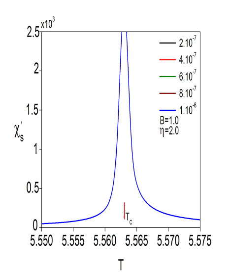
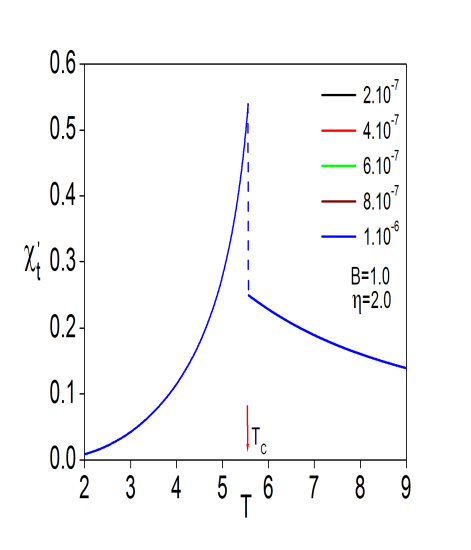
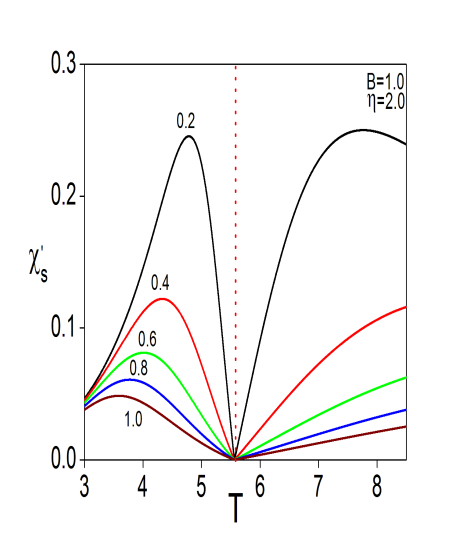
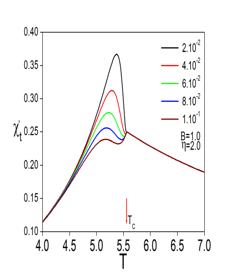
Fig.2(a)-(b) shows the critical behavior of staggered magnetic dispersion, Ο‡s′​(Ο‰)superscriptsubscriptπœ’π‘ β€²πœ”\chi_{s}^{{}^{\prime}}(\omega) and direct magnetic dispersion $\chi_{t}^{{}^{\prime}}(\omega)$ with varying temperature in the low frequency region $\omega\tau_{2}\ll 1$ . One can observe from Fig.2(a) that real part of the staggered ac susceptibility (Ο‡s′​(Ο‰)superscriptsubscriptπœ’π‘ β€²πœ”\chi_{s}^{{}^{\prime}}(\omega)) rises rapidly with increasing temperature and tends to infinity near the second order phase transition. In accordance with the expectations the staggered dispersion factor converges to static staggered susceptibility for $\omega\tau_{2}\ll 1$ (compare Fig.1(a) and Fig.2(a)). Fig2.(b) represents the temperature variation of the direct magnetic dispersion factor in the neighborhood of $T_{N}$ for $B=1.0$ and $\eta=2.0$. The real part of direct complex susceptibility increases slowly with changing temperature and makes a cusp behavior near the second order phase transition. In addition, $\chi_{t}^{{}^{\prime}}(\omega)$ converges to static direct susceptibility in the low frequency region (compare Fig.2(b) and Fig.1(b)). Moreover the behavior of Ο‡s′​(Ο‰)superscriptsubscriptπœ’π‘ β€²πœ”\chi_{s}^{{}^{\prime}}(\omega) and $\chi_{t}^{{}^{\prime}}(\omega)$ are independent of the frequency. This behavior is in accordance with results obtained for spin-1 Ising model [11].

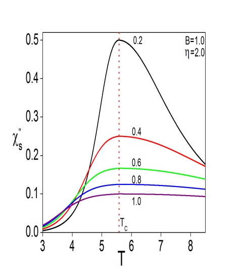
Fig. 3(a)-(b) illustrates temperature variations of staggered magnetic dispersion and direct magnetic dispersion for the high frequency region at several values of $\omega$ in the neighborhood second phase transition point. Ο‡s′​(Ο‰)superscriptsubscriptπœ’π‘ β€²πœ”\chi_{s}^{{}^{\prime}}(\omega) has a local maximum before the second order phase transition point and shows a local minimum near the critical point in the high frequency region. In these figures the number accompanying each curve denotes the value of o and the vertical arrows refer to the critical temperature for $B=1.0$ and $\eta=2.0$. The direct dispersion factor exhibits a maxima for $T\rightarrow T_{N}$ whose amplitude increases with rising frequency. This result is in parallel with findings for the total magnetic dispersion factor for the antiferromagnetic Ising model [34].

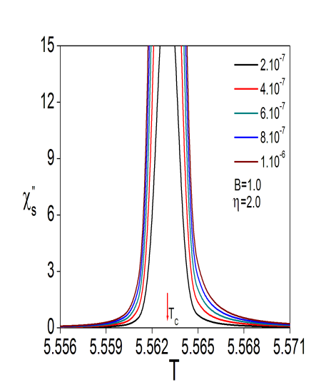
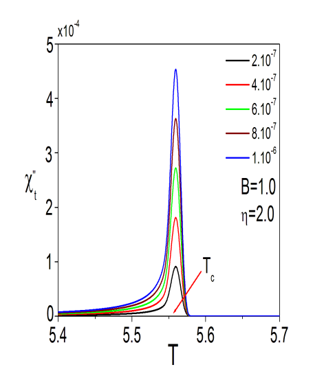
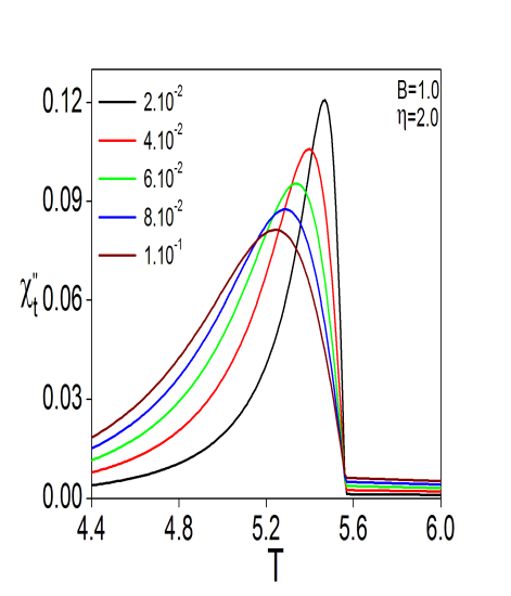
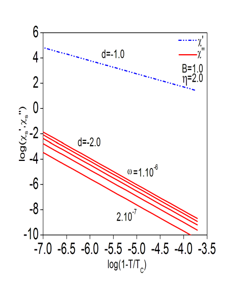
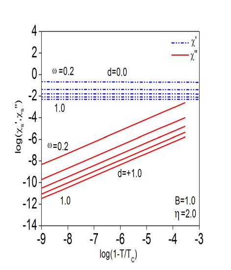
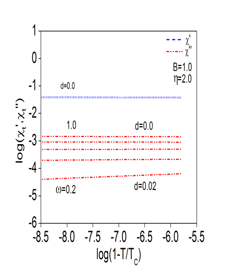
In Fig.4(a)-(b) temperature variations of staggered magnetic absorption and direct magnetic absorption are given for the low frequency region at several values of $\omega$. Ο‡sβ€²β€²superscriptsubscriptπœ’π‘ β€²β€²\chi_{s}^{{}^{\prime\prime}} exhibits a divergence, while $\chi_{t}^{{}^{\prime\prime}}$ makes a local maximum near the critical point. Fig.5(a)-(b) shows temperature variations of staggered magnetic absorption and direct magnetic absorption for the high frequency region at several values of $\omega$ in the neighborhood second phase transition point. Ο‡sβ€²β€²superscriptsubscriptπœ’π‘ β€²β€²\chi_{s}^{{}^{\prime\prime}} exhibits a local maximum at the phase transition point and amplitude of the maximum changes with frequency (See Fig. 5(a)). On the other hand, $\chi_{t}^{{}^{\prime\prime}}$ makes local minimum at the phase transition point, but it exhibits a local maximum before the critical temperature (See Fig. 5(b)). The divergencies of Ο‡s′​(Ο‰)superscriptsubscriptπœ’π‘ β€²πœ”\chi_{s}^{{}^{\prime}}(\omega) and Ο‡s′′​(Ο‰)superscriptsubscriptπœ’π‘ β€²β€²πœ”\chi_{s}^{{}^{\prime\prime}}(\omega) for $\omega\tau_{2}\ll 1$ on both sides of the critical point are characterized by the critical exponents. Thus, we may assume that, for temperatures smaller than the transition temperatures, Ο‡s′​(Ο‰)superscriptsubscriptπœ’π‘ β€²πœ”\chi_{s}^{{}^{\prime}}(\omega) and Ο‡s′′​(Ο‰)superscriptsubscriptπœ’π‘ β€²β€²πœ”\chi_{s}^{{}^{\prime\prime}}(\omega) follow laws of the form Ο‡s′​(Ο‰)∼|Tβˆ’TN|Ξ³a​cβ€²similar-tosuperscriptsubscriptπœ’π‘ β€²πœ”superscript𝑇subscript𝑇𝑁subscriptsuperscriptπ›Ύβ€²π‘Žπ‘\chi_{s}^{{}^{\prime}}(\omega)\sim|T-T_{N}|^{\gamma^{\prime}_{ac}} and Ο‡s′​(Ο‰)∼|Tβˆ’TN|Ξ³a​cβ€²β€²similar-tosuperscriptsubscriptπœ’π‘ β€²πœ”superscript𝑇subscript𝑇𝑁subscriptsuperscriptπ›Ύβ€²β€²π‘Žπ‘\chi_{s}^{{}^{\prime}}(\omega)\sim|T-T_{N}|^{\gamma^{\prime\prime}_{ac}}, respectively. Here $\gamma^{\prime}_{ac}$ and $\gamma^{\prime\prime}_{ac}$ are the dynamic critical exponents of the staggered magnetic dispersion and absorption factors. In order to calculate the mean field values of $\gamma^{\prime}_{ac}$ and $\gamma^{\prime\prime}_{ac}$, we have sketched the the plots of Ο‡s′​(Ο‰)superscriptsubscriptπœ’π‘ β€²πœ”\chi_{s}^{{}^{\prime}}(\omega) versus $log(1-\frac{T}{T_{N}})$ and Ο‡s′​(Ο‰)superscriptsubscriptπœ’π‘ β€²πœ”\chi_{s}^{{}^{\prime}}(\omega) versus $log(1-\frac{T}{T_{N}})$ which are represented in Fig.6 (a). We have found only one linear part on these $log-log$ plots for Ο‡s′​(Ο‰)superscriptsubscriptπœ’π‘ β€²πœ”\chi_{s}^{{}^{\prime}}(\omega) and Ο‡s′′​(Ο‰)superscriptsubscriptπœ’π‘ β€²β€²πœ”\chi_{s}^{{}^{\prime\prime}}(\omega), i.e., one values of $\gamma^{\prime}_{ac}$ and $\gamma^{\prime\prime}_{ac}$, respectively. For each $\omega$ value the slope of the line is equal to $-1$ for $\gamma^{\prime}_{ac}$; and $-2$ for $\gamma^{\prime\prime}_{ac}$. These values are in accordance with the diverging behavior of the magnetic dispersion and absorption factor near the second order phase transition temperature for $B=B_{0}$ and $B_{s}=B_{s_{0}}=0$. It is important to note that these findings are agreement with the critical exponents found for the magnetic spin-1 Ising model [11]. Further these results are in well agreement with the MR studies of an AB type Ising model for for Ising antiferromagnetism [34] and Ising ferromagnet [36].In addition, Fig.6(b) and (c) show logarithmic plot of staggered magnetic dispersion and staggered magnetic absorption versus reduced temperature $(1-T/T_{C})$ for $T<T_{C}$ at several values in the low frequency region and high frequency region. Finally, Table-1 represents mean field critical exponents for staggered magnetic dispersion, staggered magnetic absorbtion, direct magnetic dispersion and direct magnetic absorbtion in the low and high frequency regions.

5 Concluding Remarks

Within the mean field approximation, we have analyzed steady state solutions of the spin-$\frac{1}{2}$ metamagnetic Ising model under a time-dependent oscillating external physical and staggered magnetic fields. In this paper, the formulation is based on a method which combines the equilibrium statistical theory of critical phenomena with the theory of irreversible thermodynamics. It is assumed that the amplitude of both the physical and staggered fields are so small that we made use of linear response theory in studying the magnetic relaxation processes in a metamagnetic system. In this system there exists two coupled relaxation processes which correspond to the relaxation of ferromagnetic and antiferromagnetic order parameters. We have shown that these processes are characterized by two distinct relaxation times ($\tau_{1}$ and $\tau_{2}$ ). $\tau_{2}$ is the dominant relaxation time which characterizes the critical slowing down of the staggered magnetization and therefore the temperature variation of the second relaxation time determines the separation of the so-called low- and high-frequency regions. We should note that similar behavior has been observed in the investigation of the antiferromagnetic Ising model with the same method [34]. Since $\frac{1}{\tau_{2}}\rightarrow 0$ as $T\rightarrow T_{N}$ and keeping the frequency $\omega$ fixed, we observed the low-frequency behaviors followed by the high-frequency behaviors for the dynamic susceptibilities. One can see from Figs.2(a) and 3(a) that the slope of the staggered magnetic dispersion curve chances in sign as $T\rightarrow T_{N}$ (positive slope for the low-frequency region, negative slope for the high-frequency region). Similar behavior exists also in the high and low frequency regions for total magnetic dispersion factor. Finally, it should be emphasized that we have assumed in this study the rate coefficients have negligible temperature dependence. The validity of this assumption should be testified either by experiments or a more powerful theory such as path probability method. Kikuchi has represented an investigation of Order-disorder configurational relaxation on a bcc AB-type lattice and showed that The diagonal Onsager coefficients tend to finite values whereas the off-diagonal coefficient which characterizes the interference between coupled irreversible processes [37] tends to vanish as temperature approaches critical temperature [38].

6 Acknowledgements

This work was supported by the Scientific and Technological Research Council of Turkey (TUBITAK), Grant No. 109T721. In addition authors thank A.N. Berker for valuable discussions, Sabanci University and Massachusetts Institute of Technology

7 Appendix-A

The list of coefficients in Eqs.(6):

$$\begin{array}[]{lcl}a_{11}&=&\displaystyle 1+\frac{2\cosh(2\frac{B-m_{t}f}{k_{B}T})f}{k_{B}T\left(\cosh(2\frac{B-m_{t}f}{k_{B}T})+\cosh(2\frac{B_{s}+m_{s}t}{k_{B}T})\right)}-\frac{2\sinh(2\frac{B-m_{t}f}{k_{B}T})^{2}f}{k_{B}T\left(\cosh(2\frac{B-m_{t}f}{k_{B}T})+\cosh(2\frac{B_{s}+m_{s}t}{k_{B}T})\right)^{2}},\\ \\ a_{12}&=&\displaystyle\frac{2\sinh(2\frac{B-m_{t}f)}{k_{B}T})\sinh(2\frac{B_{s}+m_{s}t)}{k_{B}T})t}{k_{B}T\left(\cosh(2\frac{B-m_{t}f}{k_{B}T})+\cosh(2\frac{B_{s}+m_{s}t}{k_{B}T})\right)^{2}},\\ \\ a_{21}&=&\displaystyle-\frac{2\sinh(2\frac{B_{s}+m_{s}t}{k_{B}T})\sinh(2\frac{B-m_{t}f}{k_{B}T})f}{k_{B}T\left(\cosh(2\frac{B-m_{t}f}{k_{B}T})+\cosh(2\frac{B_{s}+m_{s}t}{k_{B}T})\right)^{2}},\\ \\ \end{array}$$ (35)
$$\begin{array}[]{lcl}a_{22}&=&1-\displaystyle\frac{2\cosh(2\frac{B_{s}+m_{s}t}{k_{B}T})t}{k_{B}T\left(\cosh(2\frac{B-m_{t}f}{k_{B}T})+\cosh(2\frac{B_{s}+m_{s}t}{k_{B}T})\right)}+\frac{2\sinh(2\frac{B_{s}+m_{s}t}{k_{B}T})^{2}t}{k_{B}T\left(\cosh(2\frac{B-m_{t}f}{k_{B}T})+\cosh(2\frac{B_{s}+m_{s}t}{k_{B}T})\right)^{2}},\\ \\ c_{1}&=&-\displaystyle\frac{2\sinh(2\frac{B-m_{t}f}{k_{B}T})\sinh(2\frac{B_{s}+m_{s}t}{k_{B}T})}{k_{B}T\left(\cosh(2\frac{B-m_{t}f}{k_{B}T})+\cosh(2\frac{B_{s}+m_{s}t}{k_{B}T})\right)^{2}},\\ \\ c_{2}&=&\displaystyle\frac{2\cosh(2\frac{B_{s}+m_{s}t}{k_{B}T})}{k_{B}T\left(\cosh(2\frac{B-m_{t}f}{k_{B}T})+\cosh(2\frac{B_{s}+m_{s}t}{k_{B}T})\right)}-\frac{2\sinh(2\frac{B_{s}+m_{s}t}{k_{B}T})^{2}}{k_{B}T\left(\cosh(2\frac{B-m_{t}f}{k_{B}T})+\cosh(2\frac{B_{s}+m_{s}t}{k_{B}T})\right)^{2}}.\end{array}$$
$$\begin{array}[]{lcl}b_{11}&=&1+\displaystyle\frac{2\cosh(2\frac{B-m_{t}f)}{k_{B}T})f}{k_{B}T\left(\cosh(2\frac{B-m_{t}f}{k_{B}T})+\cosh(2\frac{B_{s}s+m_{s}t}{k_{B}T})\right)}-\frac{2\sinh(2\frac{B-m_{t}f}{k_{B}T})^{2}f}{\left(\cosh(2\frac{B-m_{t}f}{k_{B}T})+\cosh(2\frac{B_{s}+m_{s}t}{k_{B}T})\right)^{2}k_{B}T},\\ \\ b_{12}&=&\displaystyle\frac{2\sinh(2\frac{B-m_{t}f}{k_{B}T})\sinh(2\frac{B_{s}+m_{s}t}{k_{B}T})t}{\left(\cosh(2\frac{B-m_{t}f}{k_{B}T})+\cosh(2\frac{B_{s}+m_{s}t}{k_{B}T})\right)^{2}k_{B}T},\\ \\ b_{21}&=&-\displaystyle\frac{2\sinh(2\frac{B_{s}+m_{s}t}{k_{B}T})(\sinh(2\frac{B-m_{t})f}{k_{B}T})f}{\left(\cosh(2\frac{B-m_{t}f}{k_{B}T})+\cosh(2\frac{B_{s}s+m_{s}t}{T})\right)^{2}k_{B}T},\\ \\ \end{array}$$ (36)
$$\begin{array}[]{lcl}b_{22}&=&1-\displaystyle\frac{2\cosh(2\frac{B_{s}+m_{s}t}{k_{B}T})t}{k_{B}T\left(\cosh(2\frac{B-m_{t}f}{k_{B}T})+\cosh(2\frac{B_{s}+m_{s}t}{k_{B}T})\right)}+\frac{2\sinh(2\frac{B_{s}+m_{s}t)}{k_{B}T})^{2}t}{\left(\cosh(2\frac{B-m_{t}f}{k_{B}T})+\cosh(2\frac{B_{s}+m_{s}t}{k_{B}T})\right)^{2}k_{B}T},\\ \\ d_{1}&=&\displaystyle\frac{2\cosh(2\frac{B-m_{t}f}{k_{B}T})}{k_{B}T\left(\cosh(2\frac{B-m_{t}f}{k_{B}T})+\cosh(2\frac{B_{s}+m_{s}t}{k_{B}T})\right)}-\frac{2\sinh(2\frac{B-m_{t}f}{k_{B}T})^{2}}{k_{B}T\left(\cosh(2\frac{B-m_{t}f}{k_{B}T})+\cosh(2\frac{B_{s}+m_{s}t}{k_{B}T})\right)^{2}},\\ \\ d_{2}&=&-\displaystyle\frac{2\sinh(2\frac{B_{s}+m_{s}t}{k_{B}T})\sinh(2\frac{B-m_{t}f}{k_{B}T})}{\left(\cosh(2\frac{B-m_{t}f}{k_{B}T})+\cosh(2\frac{B_{s}+m_{s}t}{k_{B}T})\right)^{2}k_{B}T}.\end{array}$$ (37)

8 Appendix-B

The list of coefficients in Eq.(8):

a=(βˆ‚Gβˆ‚B)e​q=βˆ’N​μ​mtb=(βˆ‚Gβˆ‚Bs)e​q=βˆ’N​μ​msc=(βˆ‚2Gβˆ‚mt2)e​q,=N​(Jβˆ’Jβ€²βˆ’14​kB​T​(βˆ’11+ms+mtβˆ’11βˆ’msβˆ’mtβˆ’11+mtβˆ’msβˆ’11βˆ’mt+ms))d=(βˆ‚2Gβˆ‚ms2)e​q,=βˆ’N​(J+Jβ€²+14​kB​T​(βˆ’11+ms+mtβˆ’11βˆ’msβˆ’mtβˆ’11+mtβˆ’msβˆ’11βˆ’mt+ms))e=(βˆ‚2Gβˆ‚B2)e​q=0,f=(βˆ‚2Gβˆ‚Bs2)e​q=0,g=(βˆ‚2Gβˆ‚mtβ€‹βˆ‚ms)e​q,=βˆ’14​kB​T​N​(βˆ’11+ms+mtβˆ’11βˆ’msβˆ’mt+11+mtβˆ’ms+11βˆ’mt+ms),h=(βˆ‚2Gβˆ‚Bβ€‹βˆ‚mt)e​q=βˆ’N​μ,i=(βˆ‚2Gβˆ‚mtβ€‹βˆ‚Bs)e​q=0,j=(βˆ‚2Gβˆ‚Bβ€‹βˆ‚ms)e​q=0,k=(βˆ‚2Gβˆ‚Bsβ€‹βˆ‚ms)e​q=βˆ’N​μ.π‘ŽsubscriptπΊπ΅π‘’π‘žπ‘πœ‡subscriptπ‘šπ‘‘missing-subexpressionmissing-subexpressionmissing-subexpression𝑏subscript𝐺subscriptπ΅π‘ π‘’π‘žπ‘πœ‡subscriptπ‘šπ‘ missing-subexpressionmissing-subexpressionmissing-subexpression𝑐subscriptsuperscript2𝐺superscriptsubscriptπ‘šπ‘‘2π‘’π‘žmissing-subexpressionmissing-subexpressionmissing-subexpressionmissing-subexpression𝑁𝐽superscript𝐽′14subscriptπ‘˜π΅π‘‡11subscriptπ‘šπ‘ subscriptπ‘šπ‘‘11subscriptπ‘šπ‘ subscriptπ‘šπ‘‘11subscriptπ‘šπ‘‘subscriptπ‘šπ‘ 11subscriptπ‘šπ‘‘subscriptπ‘šπ‘ missing-subexpressionmissing-subexpressionmissing-subexpression𝑑subscriptsuperscript2𝐺superscriptsubscriptπ‘šπ‘ 2π‘’π‘žmissing-subexpressionmissing-subexpressionmissing-subexpressionmissing-subexpression𝑁𝐽superscript𝐽′14subscriptπ‘˜π΅π‘‡11subscriptπ‘šπ‘ subscriptπ‘šπ‘‘11subscriptπ‘šπ‘ subscriptπ‘šπ‘‘11subscriptπ‘šπ‘‘subscriptπ‘šπ‘ 11subscriptπ‘šπ‘‘subscriptπ‘šπ‘ missing-subexpressionmissing-subexpressionmissing-subexpression𝑒subscriptsuperscript2𝐺superscript𝐡2π‘’π‘ž0missing-subexpressionmissing-subexpressionmissing-subexpression𝑓subscriptsuperscript2𝐺superscriptsubscript𝐡𝑠2π‘’π‘ž0missing-subexpressionmissing-subexpressionmissing-subexpression𝑔subscriptsuperscript2𝐺subscriptπ‘šπ‘‘subscriptπ‘šπ‘ π‘’π‘žmissing-subexpressionmissing-subexpressionmissing-subexpressionmissing-subexpression14subscriptπ‘˜π΅π‘‡π‘11subscriptπ‘šπ‘ subscriptπ‘šπ‘‘11subscriptπ‘šπ‘ subscriptπ‘šπ‘‘11subscriptπ‘šπ‘‘subscriptπ‘šπ‘ 11subscriptπ‘šπ‘‘subscriptπ‘šπ‘ missing-subexpressionmissing-subexpressionmissing-subexpressionβ„Žsubscriptsuperscript2𝐺𝐡subscriptπ‘šπ‘‘π‘’π‘žπ‘πœ‡missing-subexpressionmissing-subexpressionmissing-subexpression𝑖subscriptsuperscript2𝐺subscriptπ‘šπ‘‘subscriptπ΅π‘ π‘’π‘ž0missing-subexpressionmissing-subexpressionmissing-subexpression𝑗subscriptsuperscript2𝐺𝐡subscriptπ‘šπ‘ π‘’π‘ž0missing-subexpressionmissing-subexpressionmissing-subexpressionπ‘˜subscriptsuperscript2𝐺subscript𝐡𝑠subscriptπ‘šπ‘ π‘’π‘žπ‘πœ‡\begin{array}[]{lcl}a&=&\displaystyle\left(\frac{\partial G}{\partial B}\right)_{eq}=-N\mu m_{t}\\ \\ b&=&\displaystyle\left(\frac{\partial G}{\partial B_{s}}\right)_{eq}=-N\mu m_{s}\\ \\ c&=&\displaystyle\left(\frac{\partial^{2}G}{\partial m_{t}^{2}}\right)_{eq},\\ \\ &=&\displaystyle N\left(J-J^{{}^{\prime}}-\frac{1}{4}k_{B}T\left(-\frac{1}{1+m_{s}+m_{t}}-\frac{1}{1-m_{s}-m_{t}}-\frac{1}{1+m_{t}-m_{s}}-\frac{1}{1-m_{t}+m_{s}}\right)\right)\\ \\ d&=&\displaystyle\left(\frac{\partial^{2}G}{\partial m_{s}^{2}}\right)_{eq},\\ \\ &=&\displaystyle-N\left(J+J^{{}^{\prime}}+\frac{1}{4}k_{B}T\left(-\frac{1}{1+m_{s}+m_{t}}-\frac{1}{1-m_{s}-m_{t}}-\frac{1}{1+m_{t}-m_{s}}-\frac{1}{1-m_{t}+m_{s}}\right)\right)\\ \\ e&=&\displaystyle\left(\frac{\partial^{2}G}{\partial B^{2}}\right)_{eq}=0,\\ \\ f&=&\displaystyle\left(\frac{\partial^{2}G}{\partial B_{s}^{2}}\right)_{eq}=0,\\ \\ g&=&\displaystyle\left(\frac{\partial^{2}G}{\partial m_{t}\partial m_{s}}\right)_{eq},\\ \\ &=&\displaystyle-\frac{1}{4}k_{B}TN\left(-\frac{1}{1+m_{s}+m_{t}}-\frac{1}{1-m_{s}-m_{t}}+\frac{1}{1+m_{t}-m_{s}}+\frac{1}{1-m_{t}+m_{s}}\right),\\ \\ h&=&\displaystyle\left(\frac{\partial^{2}G}{\partial B\partial m_{t}}\right)_{eq}=-N\mu,\\ \\ i&=&\displaystyle\left(\frac{\partial^{2}G}{\partial m_{t}\partial B_{s}}\right)_{eq}=0,\\ \\ j&=&\displaystyle\left(\frac{\partial^{2}G}{\partial B\partial m_{s}}\right)_{eq}=0,\\ \\ k&=&\displaystyle\left(\frac{\partial^{2}G}{\partial B_{s}\partial m_{s}}\right)_{eq}=-N\mu.\end{array}

References

  • [1] P. E. Engelstad and K. Yamada, Phys. Rev. B 52 (1995) 13029.
  • [2] G. Durin, M. Bonaldi, M. Cerdonio, R. Tommasini, S. Vitale, J. Magn. Magn. Mater. 101 (1991) 89.
  • [3] M.B.F. van Raap, F.H. Sanchez, C.E.R. Torres, L. Casas, A. Roig, E. Molins, J. Phys.: Condens. Matter 17 (2005) 6519.
  • [4] J. K tzler, G. Eiselt, J. Phys. C 12 (1979) L469.
  • [5] M.A. Girtu, J. Optoelect. Adv. Mater. 4 (2002) 85.
  • [6] P.C. Fannin, C.N. Marin, I. Malaescu, A.T. Giannitsis, J. Magn. Magn. Mater. 289 (2005) 78.
  • [7] J.H. Barry, J. Chem. Phys. 45 (1966) 4172.
  • [8] J.H. Barry, D.A. Harrington, Phys. Rev. B 4 (1971) 3068.
  • [9] M. Suzuki and R. Kubo, J. Phys. Soc. Jpn. 24 (1968) 51.
  • [10] M. Acharyya, B.K. Chakrabarti, Phys. Rev. B 52 (1995) 6550.
  • [11] R.Erdem, J.Magn. Magn. Mater. 320 (2008) 2273.
  • [12] R.Erdem, J.Magn. Magn. Mater. 321 (2009) 2592.
  • [13] E.Stryjewski, N. Giordano, Adv. Phys. 26 (1977) 487.
  • [14] D.P. Landau, Phys. Rev. Lett. 28 (1972) 449; B.L. Arora, D.P. Landau, AIP Conf. Proc. 10 (1973) 870.
  • [15] F. Harbus, H.E. Stanley, Phys. Rev. B 8 (1973) 1156; F. Harbus, H.E. Stanley, Phys. Rev. B 8 (1973) 1141.
  • [16] L. Hernandez, H.T. Diep, D. Bertrand, Phys. Rev. B 47 (1993) 2602.
  • [17] Z. Onyszkiewicz, A. Wierzbicki, Physica B 151 (1988) 462.
  • [18] Z. Onyszkiewicz, A. Wierzbicki, Physica B 151 (1988) 475.
  • [19] D. Das, M. Barma, Physica A 270 (1999) 245.
  • [20] P. S. Sahni, J. D. Gunton, S. L. Katz, R. H. Timpe, Phys. Rev. B 25 (1982) 389.
  • [21] Z. R. Yang, Phys. Rev. B 46 (1992) 11578.
  • [22] E.Oguz, J. Phy. A 21 (1988) 2799 .
  • [23] G.Gulpinar, D.Demirhan, F. Buyukkilic, Physica A 383 (2007) 372.
  • [24] G.Gulpinar, D.Demirhan, F. Buyukkilic, Phys. Lett. A 373 (2009) 511.
  • [25] G. Gulpinar, D. Demirhan, F. Buyukkilic, Phys. Rev. E 75 (2007) 021104.
  • [26] G. Gulpinar, Y. Karaaslan, Phys. Lett. A, 375 (2011) 978 983.
  • [27] G. Gulpinar, Phys. Lett. A 372 (2008) 98.
  • [28] J. M. Kincaid and E. G. D. Cohen, Phys. Reports 22 (1975) 57.
  • [29] W. Selke, Z. Phys. B 101 (1996) 145.
  • [30] M. Zukovic, A. Bobak and T. Idogaki, J. Magn. Magn. Mater. 188 (1998) 52.
  • [31] M. Zukovic, A. Bobak and T. Idogaki, J. Magn. Magn. Mater. 192 (1999) 363.
  • [32] P.W. Kasteleyn, Physica 22 (1956) 387 .
  • [33] M.E. Fisher and M.F. Sykes, Physica 28 (1962) 919 ; 28, 939 (1962).
  • [34] J. H. Barry, D. A. Harrington, Phys. Rev. B 45 (1971) 3068.
  • [35] S.R. Groot and P. Mazur, Nonequilibrium Thermodynamics, Amsterdam, North Holland Pub. Co. (1961).
  • [36] J.H. Barry, J. Chem. Phys. 45 (1966) 4172.
  • [37] L. Onsager, Phys. Rev. 37, (1931) 405; 37 (1931) 2265.
  • [38] R. Kikuchi, Ann. Phys. 10 (1960) 127 ; (1963) Hughes Research Rep. No. 271.
Refer to caption
Refer to caption
Figure 1: Constant field (B) cross-sections of the staggered magnetic susceptibility (a) and direct susceptibility (b) in the neighborhood of critical point while $B=1.0$ and $\eta=\frac{zJ}{z^{\prime}J^{\prime}}$.
Refer to caption
Refer to caption
Figure 2: Temperature variations of staggered magnetic dispersion (a) and direct magnetic dispersion (b) for the low frequency region at several values of $\omega$ in the neighborhood second phase transition point.
Refer to caption
Refer to caption
Figure 3: Temperature variations of staggered magnetic dispersion (a) and direct magnetic dispersion (b) for the high frequency region at several values of $\omega$ in the neighborhood second phase transition point. The number accompanying each curve denotes the frequency.
Refer to caption
Refer to caption
Figure 4: Temperature variations of staggered magnetic absorption (a) and direct magnetic absorption (b) for the low frequency region at several values of $\omega$ in the neighborhood second phase transition point.
Refer to caption
Refer to caption
Figure 5: Temperature variations of staggered magnetic absorption (a) and direct magnetic absorption (b) for the high frequency region at several values of $\omega$ in the neighborhood second phase transition point. The number accompanying each curve denotes the frequency.
Refer to caption
Refer to caption
Refer to caption
Figure 6: Logarithmic plot of staggered magnetic dispersion and staggered magnetic absorption vs. reduced temperature $(1-T/T_{C})$ for $T<T_{C}$ at several values in the low frequency region (a) and high frequency region (b). Dotted lines are for Ο‡sβ€²superscriptsubscriptπœ’π‘ β€²\chi_{s}^{{}^{\prime}} and solid lines for Ο‡sβ€²β€²superscriptsubscriptπœ’π‘ β€²β€²\chi_{s}^{{}^{\prime\prime}}.
Table 1: Mean field critical exponents for staggered magnetic dispersion, staggered magnetic absorbtion, direct magnetic dispersion and direct magnetic absorbtion in the low and high frequency regions.
Quantity Frequency Range Exponent Value Critical Singularity
Ο‡s′​(Ο‰)superscriptsubscriptπœ’π‘ β€²πœ”\chi_{s}^{{}^{\prime}}(\omega) $2.10^{-7}-1.10^{-6}$ (low freq.) -1 divergence
Ο‡s′′​(Ο‰)superscriptsubscriptπœ’π‘ β€²β€²πœ”\chi_{s}^{{}^{\prime\prime}}(\omega) $2.10^{-7}-1.10^{-6}$ (low freq.) -2 divergence
Ο‡s′​(Ο‰)superscriptsubscriptπœ’π‘ β€²πœ”\chi_{s}^{{}^{\prime}}(\omega) $0.2-1.0$ (high freq.) 0 cusp
Ο‡s′′​(Ο‰)superscriptsubscriptπœ’π‘ β€²β€²πœ”\chi_{s}^{{}^{\prime\prime}}(\omega) $0.2-1.0$ (high freq.) +1 cusp
$\chi_{t}^{{}^{\prime}}(\omega)$ $0.2$ (high freq.) 0.02 cusp
$\chi_{t}^{{}^{\prime}}(\omega)$ $0.4-1.0$ (high freq.) 0 cusp
$\chi_{t}^{{}^{\prime\prime}}(\omega)$ $0.2-1.0$ (high freq.) 0 cusp