Temperature Variations of the Cold Dust in the Triangulum Galaxy M 33

Abstract

We present wide-field 1.1 mm continuum imaging of the nearby spiral galaxy M 33, conducted with the AzTEC bolometer camera on ASTE. We show that the 1.1 mm flux traces the distribution of dust with T$\sim 20$ K. Combined with far-infrared imaging at 160 $\mu\mathrm{m}$, we derive the dust temperature distribution out to a galactic radius of $\sim 7$ kpc with a spatial resolution of $\sim 100$ parsecs. Although the 1.1 mm flux is observed predominantly near star forming regions, we find a smooth radial temperature gradient declining from $\sim 20$ K to $\sim 13$ K consistent with recent results from the Herschel satellite. Further comparison of individual regions show a strong correlation between the cold dust temperature and the $\mathrm{K_{S}}$ band brightness, but not with the ionizing flux. The observed results imply that the dominant heating source of cold dust at few hundred parsec scales are due to the non-OB stars, even when associated with star forming regions.

1 Introduction

Galaxies are known to harbour dust components whose representative temperatures are warm ($\sim 50$ K) and cold ($\sim 20$ K). Cold dust typically represents more than $\sim 90$% of the total dust mass in galaxies (Devereux & Young, 1990). Despite the important role it plays by providing the dominant formation sites for molecular hydrogen -the fuel for star formation- relatively little is known about the spatial and temperature distribution of cold dust either in the Milky Way or in nearby galaxies.

Far-infrared (IR) flux at $\sim 25-70\ \mu\mathrm{m}$ of nearby galaxies are localized to star forming regions, and have temperatures around $\sim 50$ K; this warm component has been attributed to dust heating by UV photons from massive OB stars (Devereux et al., 1997; Hinz et al., 2004; Tabatabaei et al., 2007a). At longer wavelengths, however, the sources responsible for the dust heating becomes less evident. Dust grains with relatively large sizes $\sim 1\ \mu\mathrm{m}$ can efficiently absorb photons longer than the UV (Draine & Lee, 1984), and may be heated also by stars which are not OB stars (Xu & Helou, 1996; Bianchi et al., 2000). We will refer to these stars as non-massive stars, which may heat large dust grains but are not OB type stars. Longwards of $\sim 100\ \mu\mathrm{m}$, where the flux is sensitive to cold dust around $\sim 20$ K, the IR flux is known to be composed both from a diffuse disk component and flux concentrated near star forming regions (Hippelein et al., 2003) with both components contributing significantly to the total IR flux (Tabatabaei et al., 2007a). Gaining information on the heating sources of such cold dust, requires that we obtain a temperature distribution map of various regions in a galaxy.

Dust grains in reality have a distribution of temperatures, but far-infrared and sub-millimeter observations have suggested that as a whole, they can be characterized by two (warm and cold) representative temperatures. Measuring the temperature of dust in a galaxy requires observations at at least two wavelengths, preferably one on each side of the peak in the blackbody spectrum, which occurs around 150um for 20K dust. Far-infrared data are sensitive to warm dust emission below $\sim 100\mu\mathrm{m}$ which further hinders measurements of the temperature of the cold component (Bendo et al., 2010). A key in circumventing this problem is observations at sub-millimeter wavelengths, up to $1300\mu\mathrm{m}$. Cold dust temperatures have been derived for numerous galaxies using sub-millimeter data (e.g., Chini et al. (1995)), showing that indeed cold dust below 20 K is ubiquitous in nearby galaxies, and is distributed on a large scale in star forming disks. A major setback of current ground-based sub-millimeter observations is the lack of sensitivity to faint and diffuse emission, making large-scale mapping projects of Local Group galaxies difficult. Existing sub-millimeter observations of galaxies is therefore dominated by bright galaxies at moderate distances observed at resolution larger than several hundred parsecs (Chini & Kruegel, 1993; Chini et al., 1995; Davies et al., 1999; Alton et al., 2002; Galliano et al., 2003) which do not resolve individual star forming regions that are typically $\sim 100$ parsecs in size, or bright edge-on galaxies (Dumke et al., 2004; Weiß et al., 2008) which do not enable the clear derivation of temperature distribution within the galactic disk. Recent observations by the Herschel satellite have revealed the effectiveness of deriving temperatures using sub-mm fluxes (Bendo et al., 2010; Kramer et al., 2010).

In this paper, we explore the temperature distribution of cold dust in a nearby, nearly face-on galaxy M 33 by means of a large-scale imaging observation at 1.1 mm. The outline of this paper is as follows; section 2 describes the observation and data reduction strategy, section 3 presents the obtained image. Sections 4 presents the temperature distribution in M 33. Section 5 further compares the dust temperature with data at various other wavelengths. Section 6 summarizes the results and conclusions.

2 Observation

Observations of M 33 were conducted using the AzTEC instrument (Wilson et al., 2008), installed on the Atacama Submillimeter Telescope Experiment (ASTE) (Ezawa et al., 2004; Kohno, 2005; Ezawa et al., 2008), a 10m single dish located in the Atacama desert of altitude 4800m in Pampa La Bola, Chile. Observations were remotely made from an ASTE operation room of the National Astronomical Observatory of Japan (NAOJ) at Mitaka, Japan, using a network observation system N-COSMOS3 developed by NAOJ (Kamazaki et al., 2005). Basic parameters of M 33 are listed in table 1.

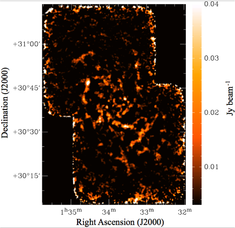
Figure 1: M 33 observed with AzTEC/ASTE.

Two square fields covering the northern and southern half of M 33, each $30^{\prime}\times 30^{\prime}$ and overlapping by $20^{\prime}\times 5^{\prime}$, where observed at 1.1 mm (270 GHz) (see figure 1). At this wavelength, the array field of view of AzTEC is $7.5^{\prime}$ with a detector FWHM of $28^{\prime\prime}$. The field was raster-scanned in the right ascension and declination direction alternately, in steps of $30^{\prime\prime}$ at a scan speed of $180^{\prime\prime}\mathrm{sec}^{-1}$. Since the AzTEC detectors are arranged in a hexagonal pattern, this scan step results in a Nyquist-sampled sky with uniform coverage.

Observations were conducted in July 2007 and August 2008, during a total observing time of 40 hours including calibration and pointing overheads. Approximately 30 hours were spent on-source. The zenith opacity at 220 GHz ranged from 0.01 to 0.2, with an average of 0.06.

Telescope pointing was monitored every two hours using the bright quasar J0238+166. The pointing was accurate to $2^{\prime\prime}$ during the observing runs. Uranus or Neptune was observed twice per night in order to measure the relative detector pointing offsets and their point spread functions. These measurements are also used for determining the absolute flux calibration. Relative flux calibration error is estimated from the flux variation of J0238+166, which was 10%. Since J0238+166 is a variable source, this represents a conservative overestimate of the calibration error. Adding in quadrature with the 5% uncertainty in the brightness temperature of Uranus (Griffin & Orton, 1993), the total absolute flux calibration error is better than 11%. The effective beamsize after beam-smoothing the reduced maps, was $40^{\prime\prime}$.

2.1 Data Reduction

Since the raw signals at 1.1 mm are dominated by atmospheric emission, we removed the atmospheric signals using an adaptive principal component analysis (PCA) technique (Scott et al., 2008). The PCA method identifies and subtracts the common-mode signal seen across the bolometer array for each scan. The PCA calculation is done in the time-domain data, then each scans are mapped and co-added to obtain the final image. Noise is estimated by “jack-knifing” the individual datasets (that is, multiplying each individual time-stream scans randomly by +1 or -1) before the map making. This cancels out true astronomical signals while preserving the noise properties of the map, resulting in a realistic representation of the underlying noise. Details of the PCA method are explained in Scott et al. (2008).

The PCA method is optimized for the detection of point sources, by subtracting any extended signals as atmospheric emission. Therefore, extended emission from M 33 will also be largely subtracted in this process. We use an iterative flux recovery approach called FRUIT to retrieve extended emission from M 33. The algorithm is briefly explained below.

The idea of the iterative flux recovery approach has already been implemented (Enoch et al., 2006) on Bolocam, a bolometer identical to AzTEC, on the Caltech Submillimeter Observatory (CSO). The FRUIT code used in this study was developed by the AzTEC instrument team at University of Massachusetts (UMass), and explained in Liu et al. (2010).

Structures with scales larger than a several arcmin are removed by the PCA technique because they introduce a correlated signal to the detectors which is indistinguishable from atmospheric variations. The residual image created by subtracting the PCA cleaned data from the original dataset therefore still contains true astronomical signals which are more extended than what is obtained from PCA cleaning. The FRUIT algorithm utilizes this residual data, by PCA cleaning them again and adding the result to the initial result of PCA. The idea is somewhat analogous to the CLEAN method (Högbom, 1974) used commonly in interferometric observations at mm wavelengths.

The observed map of the AzTEC instrument in scan $i$, $M_{i}$, can be categorized into three types of signals. These are the atmospheric signal $A_{i}$, the true astronomical signal $S$, and noise $N_{i}$. Note that the astronomical signal is independent of scan. Although $S$ is the parameter we wish to derive, we can only construct the best estimator for $S$ using various algorithms, which we write $\tilde{S}$. In PCA, we construct an estimator $\tilde{S_{i}}$ from $m_{i}$ (where the lower case represents the time-domain analog of the upper case maps), and co-add these $\tilde{S_{i}}$ to obtain $\tilde{S}$. The FRUIT algorithm works iteratively in the following way;

1. Construct $\tilde{S_{i}}$ from $m_{i}$ using PCA.

2. Construct $\tilde{S}$ by co-adding $\tilde{S_{i}}$. This is where PCA finishes.

3. Construct a residual, $\tilde{r_{i}}=m_{i}-\tilde{s}$. Ideally, this should be astronomical signal free. In practice, it still contains extended emission.

4. PCA clean the residual $\tilde{r_{i}}$ and obtain map $\tilde{R}$

5. Construct the new estimator, $\tilde{S^{\prime}}=\tilde{S}+\tilde{R}$.

6. Go back to step 3. The iteration continues until no pixels have signal-to-noise of over 3.5.

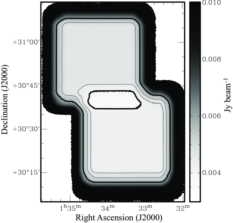
Figure 2: Noise map of M 33. The contours are drawn at 4.0, 4.5, 5.0 and 6 $\mathrm{mJy\ beam^{-1}}$, from the center outwards.

The 1.1 mm image obtained from the FRUIT algorithm is shown in figure 1, and the noise map obtained by jack-knifing the residual maps in figure 2.

This algorithm was tested by embedding two dimensional Gaussian components with FWHM of $1^{\prime}$, $2^{\prime}$, and $3^{\prime}$ and various peak intensities in the original data, and measuring the fraction of the extended flux recovered with this iterative cleaning method. We find that this technique retrieves 90% of the flux in extended structures up to $2^{\prime}$, and $\sim 60\%$ for structures with angular sizes of $3^{\prime}$. Results of this test are summarized in table 2. The results are consistent with the same test done in Shimajiri et al. (2011), and shows that the 1.1 mm flux obtained at the scale of few arcminutes are reasonable.

The northern and southern halves of the galaxy were mapped using FRUIT individually, and then merged by weighting the overlapping region by the inverse square of their noise level. Regions with less than 50% coverage in each of the northern and southern halves were clipped from further analysis.

The final maps are constructed at $6^{\prime\prime}$ per pixel. The root mean square (r.m.s.) of the resulting noise map is $3.7-4.0\ \ \mathrm{mJy\ beam^{-1}}$ in the central $\sim 100\ \mathrm{arcmin^{-1}}$, increasing to $4.3-4.7\ \ \mathrm{mJy\ beam^{-1}}$ in the outermost regions where scientific analysis is conducted (see figure 2).

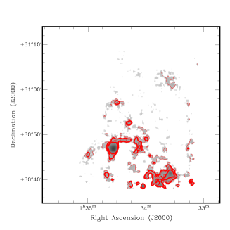
Figure 3: Left: Input Spitzer MIPS 160 $\mathrm{\mu m}$ image, scaled to AzTEC fluxes. Contours are drawn from 15 $\mathrm{mJy\ beam^{-1}}$ in steps of 5 $\mathrm{mJy\ beam^{-1}}$. Right: Output Spitzer MIPS 160 $\mathrm{\mu m}$ map, after applying PCA and FRUIT. Contour steps are same as the left panel. The southern most edge with a coverage of $<$ 50% of the peak is clipped.

As a further test of how much extended emission is recovered in the reduction, we apply the same technique as in Liu et al. (2010), by applying the FRUIT algorithm to Spitzer $160\ \mathrm{\mu m}$ data (see section 4.1) to see the level of flux loss. The test was done on the northern half of M 33. The Spitzer data were first scaled so that the flux level was similar to AzTEC data, to ensure that the same filtering was applied. The scaled data were then added to the AzTEC noise map in the time-stream domain, and then the PCA and FRUIT algorithms were applied. The left and right panels of figure 3 show the MIPS map prior to and following the PCA+FRUIT reduction, respectively . The most extended features at scales over $5^{\prime}$ are clearly subtracted out, but smaller scale features $<5^{\prime}$ are retrieved. The total flux recovered by FRUIT was 54% of the input flux, but when restricted to pixels with S/N over 2 in the FRUITed image, 97% of the total flux was recovered.

Figure 4 shows the output flux as a function of input flux, only for pixels with a local S/N over 2 in the output map. The 1$\sigma$ standard deviation of the points in figure 3 around the line of unity is 44%. Although this is a simulation using MIPS images, we regard this as a representative uncertainty of the flux measurements in the AzTEC map. It is likely to be an overestimate of scatter, because millimeter emission is often more clumpy than at far-IR; clumpy structures are retrieved by FRUIT more efficiently than smooth features. Added in quadrature with the absolute calibration error of 11% (section 2), the pixel based flux uncertainty of the M 33 map is 45% after PCA+FRUIT reduction. The simulation implies that smaller scale structures (typically smaller than $3^{\prime}$) retrieved in the PCA+FRUIT are accurate to this uncertainty and recovered to 97% if detected at S/N over 2, but larger scale features are subtracted out and are not quantified by the 45% uncertainty.

3 Results

Figure 5 shows the obtained 1.1 mm contour map of M 33, overlaid on a narrow-band H$\alpha$ image. At the distance of 840 kpc for M 33 (Freedman et al., 1991), the angular resolution of $40^{\prime\prime}$ corresponds to $160$ pc.

A clear spiral pattern is observed, coincident with the optical arms. The 1.1 mm continuum is detected out to a radius of $\sim 7$ kpc, which is coincident with the edge of the star forming disk (Verley et al., 2009). Almost all of the 1.1 mm clumps are observed to be associated with star forming regions as seen in the H$\alpha$. This is consistent with previous observations in the far-IR (Devereux et al., 1997; Tabatabaei et al., 2007a). An extended disk is not observed, however, presumably due to the subtraction of extended features during the data reduction process. Although the global 1.1 mm morphology is similar to that seen in H$\alpha$, the contamination of free-free bremsstrahlung to 1.1 mm is expected to be negligible.

For optically thin HII regions observed at frequencies higher than few Hz, the free-free emission can be written in the form;

$$F_{\nu}^{\mathrm{ff}}\propto\mathrm{N_{e}T_{e}}\nu^{-0.1}$$ (1)

where $\mathrm{N_{e}}$ and $\mathrm{T_{e}}$ are the electron number density and electron temperature of the HII region, respectively. Tabatabaei et al. (2007b) observed M 33 at $3.6$ cm ($8.3$ GHz), where the flux is dominated by synchrotron radiation and thermal free-free emission. From Tabatabaei et al. (2007b), the typical $3.6$ cm emission seen in the HII regions have peak fluxes of $\sim 10\ \mathrm{mJy\ beam^{-1}}$. Taking into account the typical thermal fraction of HII regions as $\sim 50\%$ (Tabatabaei et al. (2007c)), and scaling by equation 1, we obtain the $1.1\$mm flux estimate of free-free emission at HII regions, of $3.5\ \mathrm{mJy\ beam^{-1}}$. This is barely detectable with the r.m.s noise of our observations, which goes down to $3.7\ \mathrm{mJy\ beam^{-1}}$. For regions which we will discuss in the following sections, the $1.1\$ mm flux is typically $\sim 30\ \mathrm{mJy\ beam^{-1}}$. Therefore, the free-free contribution to the $1.1\$ mm flux is at most around $12\%$. We will therefore assume hereafter that the $1.1\$mm flux is the pure flux from the cold dust continuum.

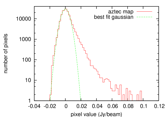
Figure 6: The probability density function (PDF) of the AzTEC map. The red histogram shows the PDF, and the dashed green line shows the best fit gaussian using pixels below $15\ \mathrm{mJy\ beam^{-1}}$.

The number probability density function (PDF; distribution of fluxes values in each pixel) of the whole AzTEC map was used to obtain a realistic estimate of the total 1.1 mm flux. This was done in place of the normal aperture photometry, in order to circumvent the possibility of including significant negative pixels in the total flux which can be added by the PCA method. It can also deal with large scale correlated noise, which may have systematic effects on the total flux. Figure 6 shows the PDF of the AzTEC map, clipped where the r.m.s. noise level exceeded $6\ \mathrm{mJy\ beam^{-1}}$, within which we have done any analysis. The faint end of the distribution, dominated by noise, is well fitted by a gaussian with a dispersion of $6.0\ \mathrm{mJy\ beam^{-1}}$. This shows that any negative pixels introduced by the PCA method and FRUIT retrievals, are offset by any positive values introduced, so that the sum of all the pixels in the AzTEC image still represents the true observed total flux of M33 reasonably well. The sum of all pixels with values larger than $-15\ \mathrm{mJy\ beam^{-1}}$, or about -3 $\sigma$, was 10.0 Jy. Including all pixels below $-15\ \mathrm{mJy\ beam^{-1}}$, the total flux is 9.9 Jy. No pixels had values lower than $-20\ \mathrm{mJy\ beam^{-1}}$. The flux retrieval simulation using MIPS measurements in the previous section showed that FRUIT retrieved $\sim$ 50% of the total flux when no restrictions to the signal-to-noise ratio are given, so the intrinsic $1.1\$ mm flux is be estimated to be $\sim$ 20 Jy, which can be regarded as the flux upper limit. Therefore, a range of $9.9-20$ Jy gives a reasonable estimate of the total observed $1.1\$ mm flux of M 33.

4 Temperature Distribution

4.1 Spitzer MIPS 160um Data

We retrieved the $160\ \mu\mathrm{m}$ Multiband Imaging Photometer (MIPS: Rieke et al. (2004)) datasets (AORs 3648000, 3648256, 3649024, 3649280, 3650048, 15212032 and 15212288) of the Basic Calibrated Data (BCD) created by Spitzer Science Center (SSC) pipeline from the Spitzer Space Telescope (Werner et al., 2004) data archive. Individual frames were processed using MOPEX (Makovoz & Khan, 2005) version 18.4, rejecting outliers and background-matching overlapping fields. Each mosaics of dimension $100^{\prime}\times 20^{\prime}$ were co-added using WCS coordinates. The co-added image was then background-subtracted by selecting several regions away from M 33 (by more than $30^{\prime}$), fitting, interpolating and subtracting a first order plane. The 1$\sigma$ background noise level was measured at several regions well away from the disk of M 33, which was at most $0.9\ \mathrm{mJy\ Str^{-1}}$ per $8^{\prime\prime}$ pixel.

The flux error of $160\ \mu\mathrm{m}$ is the sum of the error in zero-point magnitude of $1.5\%$, and in the conversion from instrumental units to $\mathrm{MJy\ Str^{-1}}$ of $12\%$ (both from Spitzer Science Center Home-page). Additionally, the background noise level of $0.9\ \mathrm{MJy\ Str^{-1}}$ must be taken into account. The weakest features for which the temperature was derived (in the outermost disk) has a $160\ \mu\mathrm{m}$ intensity of $\sim 10\ \mathrm{MJy\ Str^{-1}}$, so background noise can account for up to $\sim 10\%$. All errors taken into account, the pixel-to-pixel $160\ \mu\mathrm{m}$ flux should be accurate to $\leq\sqrt{1.5\%^{2}+12\%^{2}+10\%^{2}}=16\%$. The angular resolution (FWHM) of the point spread function is $40^{\prime\prime}$.

4.2 Global Temperature

The total $160\ \mu\mathrm{m}$ flux measured within a $60^{\prime}$ aperture (regions inside the aperture but outside the observed region were masked by null) was $\sim 1900\ \mathrm{Jy}$, well within the uncertainties of the measurements by Hinz et al. (2004), $2054\pm 411\ \mathrm{Jy}$, so the MIPS data reduction presented in the previous section is consistent with other studies in the literature. In the SED fit explained below, we use the $160\ \mathrm{\mu m}$ value by Hinz et al. (2004). Far-IR flux measurements at other wavelengths are listed in table 3. The far-IR SED is known to be successfully represented by two-component modified blackbodies shortwards of 500 $\mathrm{\mu m}$ in various regions within the galaxy (Kramer et al., 2010), and we assume a two-component spectrum also. This assumption can break down if there is significant contribution from the free-free thermal component at the long wavelengths (but see section 3), or significant contribution from non thermal-equilibrium dust (very small grains with small heat capacity) exist at the shortest wavelengths $\sim$ 24 $\mathrm{\mu m}$ (Hippelein et al., 2003).

The flux $F_{\nu}$ at various IR bands were fitted with a two-component modified blackbody model of the form

$$F_{\nu}=\nu^{\beta}\{aB_{\nu}(\mathrm{T_{w}})+bB_{\nu}(\mathrm{T_{c}})\}$$ (2)

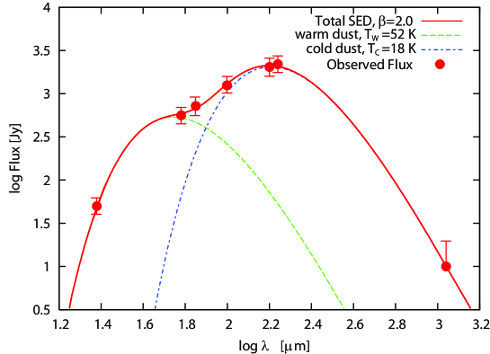
Figure 7: Two component fit to the observed global SED of M 33. The green dotted curve is the warm dust component with temperature $\mathrm{T_{w}}=52\pm 7$ (K), and the blue dash-dotted curve is the cold dust component with temperature $\mathrm{T_{c}}=18\pm 3$ (K), using the observed 1.1 mm flux of 10 Jy. The red solid curve is the sum of the two components. Errors in the infrared fluxes are typically 20%, and are taken from Hippelein et al. (2003) and Hinz et al. (2004). For the 1.1 mm flux, explanation of errors are given in section 3.

where $a$ and $b$ are constants, $\beta=2.0$ is the assumed dust emissivity index , and $B_{\nu}(\mathrm{T})$ is a Planck function at temperature T. The chi-square fitted result is shown in figure 7. We obtained $\mathrm{T_{w}}=52\pm 7$ K, $\mathrm{T_{c}}=18\pm 3$ K and $\chi^{2}=0.5$, where $\chi^{2}$ is the reduced chi-square value. For a single component modified blackbody with varying $\beta$, we obtain $\mathrm{T}=56\pm 10$ K, $\beta=0.2\pm 0.5$, and $\chi^{2}=13$, so this high reduced chi-square value rules out a single component modified blackbody spectrum. Considering the uncertainty of $\beta$ and that many previous studies have derived $\beta\sim 2$ (Knacke & Thomson, 1973; Draine & Lee, 1984; Gordon, 1988; Mathis & Whiffen, 1989; Chini & Kruegel, 1993; Kruegel & Siebenmorgen, 1994; Lis & Menten, 1998; Dunne et al., 2000; Dunne & Eales, 2001; Hill et al., 2006; Kramer et al., 2010), we keep $\beta=2.0$ constant hereafter.

Our derived global cold dust temperature $\mathrm{T_{c}}$ should be considered an slight overestimate, since extended features are subtracted in the data reduction (see section 2.1). If we use the corrected 1.1 mm flux estimate of 20 Jy, we obtain a cold dust temperature of $16\pm 2$ K. This temperature and the corrected 1.1 mm flux is consistent with extrapolations of the far-IR SED to 1.1 mm in previous measurements (Hippelein et al., 2003) and the recent value derived from Herschel (Kramer et al., 2010).

Using the observed 1.1 mm flux of 10 Jy and cold dust temperature of 18 K, and assuming optically thin dust and a dust emissivity of $\kappa=0.114\ \ \mathrm{m^{2}\ kg^{-1}}$ (Ossenkopf & Henning, 1994), we obtain a total observed dust mass of $1\times 10^{6}\ \ \mathrm{M_{\odot}}$. For an estimated intrinsic flux of 20 Jy and the resulting temperature of 16 K, the dust mass becomes $2.8\times 10^{6}\ \ \mathrm{M_{\odot}}$.

The neutral atomic mass is $1\times 10^{9}\ \ \mathrm{M_{\odot}}$ (Newton, 1980) and the molecular gas mass is estimated to be $2.6\times 10^{8}\ \ \mathrm{M_{\odot}}$ from CO observations (Heyer et al., 2004), so the total dust-to-gas ratio is derived to be $\sim 500-1300$.

An important indication from figure 7 is that the two different temperature components both contribute significantly at wavelengths around and below $100\ \mu\mathrm{m}$, whose fluxes combined with fluxes $\geq 100\ \mu\mathrm{m}$, are used commonly to discuss the temperatures of the cold dust component. This can significantly overestimate the cold dust temperature. Verley et al. (2009) gave a cold dust temperature declining from $\sim 25\$K to $\sim 21\$K in M 33 using the color temperature of $70\ \mu\mathrm{m}$ combined with $160\ \mu\mathrm{m}$, but at $70\ \mu\mathrm{m}$, figure 7 shows that the two dust components contribute almost equally. Bendo et al. (2010) and Kramer et al. (2010) also show that wavelengths shortwards of $100\mu\mathrm{m}$ are contributed significantly by star formation. Although color temperatures derived using only the two bands $\sim 160\ \mu\mathrm{m}$ and $1100\ \mu\mathrm{m}$ can still suffer from variations in $\beta$ (see section 4.5), it gives a more reasonable representation of the colder component and its characteristic temperature $\mathrm{T_{c}}$ compared to attempts using shorter wavelengths.

4.3 Color Temperature

The color temperature was derived using

$$\mathrm{R}\equiv\frac{F_{160\ \mu\mathrm{m}}}{F_{1100\ \mu\mathrm{m}}}=\left(\frac{1100}{160}\right)^{-\beta}\frac{B_{160}(T)}{B_{1100}(T)}$$ (3)

which is obtained from equation (2) at two wavelengths, for a single temperature component. Equation (3) was solved numerically to obtain the correspondence between observed flux ratio and the color temperature, and interpolated to the observed ratios. Uncertainties were estimated from the flux uncertainties in the 1.1 mm flux of 45% (section 2) and 160 $\mathrm{\mu m}$ of 16% (section 4.1), which added in quadrature results in an flux ratio uncertainty estimate of 48%. At temperatures of 10 K, 18K, and 20 K, the flux ratio $\frac{F_{160\ \mu\mathrm{m}}}{F_{1100\ \mu\mathrm{m}}}$ is 20, 120, and 160, corresponding to color temperature uncertainties of 0.9 K, 2.3 K, and 2.8 K, respectively.

In the actual derivation, the region corresponding to the observed AzTEC field was cut out from the $160\ \mu\mathrm{m}$ image, and further re-gridded to the same pixel size ($6^{\prime\prime}\mathrm{pix}^{-1}$). The Spitzer field of view did not include the northeastern and southwestern edge regions, and are excluded from temperature analysis.

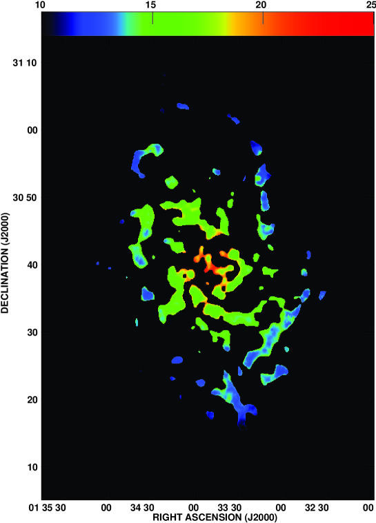
Figure 8: The cold dust temperature map of M 33. Units are in $\mathrm{T_{c}}$(K).

The two images were then divided pixel-by-pixel, using only those pixels where $1.1\$mm fluxes exceeded $6.0\ \mathrm{mJy\ beam^{-1}}$ (the characteristic 1$\sigma$ noise level of the map, but $\geq 1.5\sigma$ for most cases. See figure 2.) and $160\ \mu\mathrm{m}$ flux exceeded the $1\sigma$ noise level of $0.9\ \mathrm{mJy\ str^{-1}}$, to ensure that the flux ratios are not affected by noise (virtually no cuts were made for $160\ \mu\mathrm{m}$ data using this criterion, however; all regions where the map satisfied the $1.1\$mm criterion had $\sim 10\sigma$ in the Spitzer map). The flux ratios were then converted into temperature using the numerical solution to equation 3. The obtained cold dust temperature map is shown in figure 8. The color temperature derived for the global flux was 21 K for the total observed flux of 10 Jy, and 18 K for the estimated total intrinsic flux of 20 Jy. These values are within the uncertainties presented for temperature derivation using two-component modified blackbody fits in section 4.2.

A prominent feature evident from the temperature map, is that the local variation of temperature at small scales of several arcminutes ($1^{\prime}=240$pc) is small compared to the global variation seen at kpc scales, namely the temperature decrease observed from the center outwards. Only a few intense star forming regions are found to have temperatures slightly higher than the surrounding dust, and the bulk of dust seems to be at temperatures that follow a global trend. This is unexpected in the case where recent star formation governs the dust temperature, because star formation varies its intensity at small scales. The smooth distribution of temperatures despite the range of star formation intensities in these regions, show that the observed concentration of 1.1 mm flux nearby star forming regions is simply the result of more dust being there, not a higher temperature.

For each of the arcminute-sized clumps in the map, the temperature seem to be higher at the edges compared to the inner regions. This may be caused by the data reduction procedure, since the flux retrieval fraction of extended features decrease with increasing source size. At large scales, the 1.1 mm flux is underestimated, giving a higher temperature.

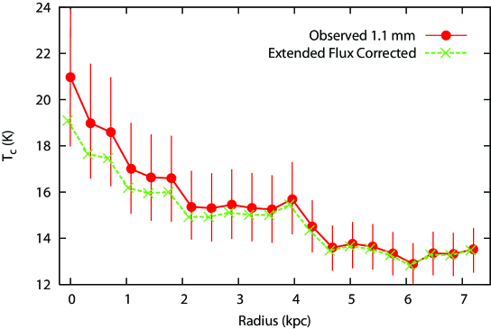
Figure 9: The cold dust temperature gradient. Red circles are the temperature derived from observed flux ratios. Green crosses are temperatures after the correction for extended flux loss, explained in section 4.4. Errorbars are determined from flux uncertainties in the observations (see section 4.3).

Figure 9 shows the radial temperature gradient, constructed from figure 8 averaged over radial bins of $90^{\prime\prime}$ width, which is chosen to mitigate the effect of temperature variations at the edges of arcminute structures. The declining temperature gradient is clearly apparent. Only a few cold dust temperature gradients have previously been found (e.g., Kramer et al. (2010)). It is important to note that this gradient is found even though the 1.1 mm emission is found predominantly where star formation is active; even for dust associated with star forming regions at $\sim 100$ pc scales, M 33 has a smooth temperature gradient which varies globally.

4.4 Correction for Extended Emission

As discussed in section 2.1, the total flux retrieved by FRUIT for Spitzer $160\mu\mathrm{m}$ data was 54%. We can also assumed this to be the fraction of flux lost in the 1.1 mm data analysis, i.e., $\sim$ 10 Jy (section 3). Such 1.1 mm flux would reside in extended structures typically over $5^{\prime}$, corresponding to $\sim$ 1.2 kpc. Extended dust disks of kilo-parsec size have been detected in the sub-millimeter range Meijerink et al. (2005), and the existence of such a structure in M 33 would be the obvious candidate of structures which may be lost in the data processing. If this extended dust disk had a radially declining flux distribution, more 1.1 mm flux would be lost in the central regions, giving a higher dust temperature when compared with $160\mu\mathrm{m}$ data. This can mimic a temperature gradient. Below we attempt to estimate that this effect can have on our derived temperature gradient.

We assume here that the total flux missed by 1.1 mm data analysis is 10 Jy, and that it forms a smooth exponential disk as in Meijerink et al. (2005), with a scale radius of 2.4 kpc as derived from both the $160\mu\mathrm{m}$ (Verley et al., 2009) and CO observations (Heyer et al., 2004). An exponential disk gives more extended flux to the central region, thus can be considered to be the worst case scenario, while giving a physically plausible model. The dust temperature was recalculated by accounting for this model in the 1.1 mm flux for the flux ratio R in equation (3). The resulting temperature profile is shown as green dashed lines in figure 9. Although the temperature decreases in the central few kpc by 1-2 K, a radial decline is still apparent.

4.5 Variation in $\beta$

Properties of dust grains (i.e., size distribution and optical properties) are usually expressed in terms of their dust grain emissivity index $\beta$. Although we have used a fixed $\beta$ for our analysis, grain properties and their size distribution may vary within a galaxy thus changing $\beta$; this corresponds to the case where a two temperature decomposition of the SED is not valid, and must include a range of temperatures. This is expected theoretically (Li & Draine, 2001; Dale & Helou, 2002), and a wide range of dust temperatures have actually been observed in our Galaxy (Reach et al. (1995)).

Variations in $\beta$ can alter the derived cold dust temperature. In particular, a radial variation in $\beta$ may be able to mimic a temperature gradient. For the temperature gradient in figure 9 to be entirely explained instead by a constant temperature at 20 K and variation in $\beta$, $\beta$ must be $\sim 2$ in the central regions and decreasing to $\beta\sim 1$ in the outer several kilo-parsecs. Although variations in $\beta$ are known to be $2\pm 0.6$ (Hill et al., 2006) in the Milky Way, systematic variations with respect to regions within a galaxy have not been reported. Furthermore, low values of $\beta$ around 1 - 1.5 are typically found near individual proto-stars (Weintraub et al., 1989; Knapp et al., 1993; Williams et al., 2004). It is unlikely that the characteristics of dust found in such circumstellar environments dominate over the outer region of M33 at kilo-parsec scales. Although small radial variations in $\beta$ cannot be ruled out with our current dataset, a global temperature gradient seems to more plausibly explain the flux ratio gradient between 1.1 mm and 160$\mu\mathrm{m}$.

5 Temperature - $\mathrm{K_{S}}$ - H$\alpha$+24$\mu\mathrm{m}$ Correlation

In order to assess the heating sources of cold dust within sub-regions of the galaxy, we performed aperture photometry around individual HII regions, and compared the dust temperature with properties at various wavelengths.

The $\mathrm{K_{S}}$ band ($2.1\mu\mathrm{m}$) can be used to trace the stellar distribution and the contribution of non-massive stars to the interstellar radiation field which heats the dust. The $\mathrm{K_{S}}$ band image of M 33 was taken from the $2MASS$ Large Galaxy Survey catalog in the NASA/IPAC Infrared Science Archive. The image was background subtracted using a planar fit to regions well away from the galaxy. The $\mathrm{K_{S}}$ band flux can be contaminated by a variety of sources other than non-massive stars. They are the nebular and molecular emission lines (Hunt et al., 2003), and hot dust (Devost, 1999). Observations of star clusters have found that star clusters can have excess H-K colors due to these contributors by at most 0.5 magnitudes (Buckalew et al., 2005). We thus apply this conservative estimate of 0.5 magnitudes (40%) on the errorbar for the stellar component of the $\mathrm{K_{S}}$ flux.

The ionizing flux from massive (OB) stars cannot be measured directly because of severe Ly$\alpha$ extinction, but we may estimate the measure of the number of OB stars by a combination of H$\alpha$ and 24$\mu\mathrm{m}$ warm dust continuum, as done by Calzetti et al. (2007) to derive extinction-corrected star formation rates. The H$\alpha$ image is from Hoopes & Walterbos (2000), and the 24$\mu\mathrm{m}$ from the Spitzer archive. The scale factor when adding H$\alpha$ and 24$\mu\mathrm{m}$ is 0.031, given by Calzetti et al. (2007) in order to minimize the dispersion of the combined star formation rate to that derived from Pa$\alpha$ flux. The dispersion is 20%, which we take to be the uncertainty in the measure of ionizing flux. Uncertainties from aperture photometry were negligible compared to 20%. Details of the data reduction and preparation for the 24$\mu\mathrm{m}$ image is found in Onodera et al. (2010).

The HII regions to perform aperture photometry on were searched from the literature with spectroscopic Oxygen abundances (Vilchez et al., 1988; Crockett et al., 2006; Magrini et al., 2007; Rosolowsky & Simon, 2008). A box with $54^{\prime\prime}$ on the side and centered on the HII region coordinate, was used to locate the flux weighted center of each of the images within that box. This centroid pixel was used as the center of the photometric apertures. This is because dust peaks are not always coincident with the H$\alpha$ or $\mathrm{K_{S}}$ peaks, typically by several to $\sim 10^{\prime\prime}$ , corresponding to under 40 parsecs. All regions were then inspected by eye to ensure that the measured emission was associated with the HII region.

Flux from a total of 57 regions were measured in each of the 1.1 mm, 24 $\mu\mathrm{m}$, 160$\mu\mathrm{m}$, H$\alpha$ and $\mathrm{K_{S}}$ band images each using a circular aperture with a radius of $36^{\prime\prime}$. The cold dust temperature was derived from the 1.1 mm, 160$\mu\mathrm{m}$ using integrated fluxes from the photometry. No local background was subtracted using an annuli in the photometry process, because most of the sources measured here are both crowded and extended. An aperture correction factor of 1.745 , taken from the MIPS Instrument Handbook Version 2.0, was applied to the 160 $\mathrm{\mu m}$ photometry, for 30 K dust with no sky annulus subtraction.

Figure 10 shows the relation between cold dust temperature, $\mathrm{K_{S}}$ band, and the measure of ionizing flux. A clear correlation is seen between the cold dust temperature T and $\mathrm{K_{S}}$ flux. The correlation coefficient $r^{2}$ is 0.71. Conversely, the correlation between T and ionizing flux is less evident, with $r^{2}=0.26$. Uncertainties in aperture photometry or temperature are not sufficient to explain the difference in the dispersion. The fact that ionizing flux from massive stars do not correlate with the dust temperature implies that these stars are not responsible for heating the dust observed here, whereas stars seen in the correlated $\mathrm{K_{S}}$ band are a strong candidate for dust heating. Although flux from the Rayleigh-Jeans tail of the ionizing stars can potentially contribute also to the $\mathrm{K_{S}}$ band, they cannot be the major dust heating source in this case, because if so the correlation should be strong both in $\mathrm{K_{S}}$ and the ionizing flux. Similarly, the contribution of diffuse H$\alpha$ and 24$\mathrm{\mu m}$ emission to the photometry, likely due to energy input from evolved stars (Verley et al., 2007), cannot explain a stronger correlation between cold dust temperature T and $\mathrm{K_{S}}$ flux, compared to the combined H$\alpha$ and 24$\mathrm{\mu m}$.

This lends strong support to non-ionizing stars as the heating source of cold dust, even in the small scale star forming regions discussed here.

6 Summary and Conclusions

This paper presented a large scale 1.1 mm mapping observation of M 33, the most proximate face-on spiral galaxy in the Local universe. The 1.1 mm continuum is detected out to $\sim 7$ kpcs, where the edge of the star forming disk lies. By comparing the 1.1 mm data with Spitzer MIPS 160$\mu\mathrm{m}$ imaging, we obtained the color temperature distribution of cold dust, without significant contribution from warm dust as in most previous studies. Furthermore, aperture photometry was performed on star forming regions to compare the cold dust temperature with $\mathrm{K_{S}}$ band flux, representing radiation from non-massive stars, and H$\alpha$+$24\mu\mathrm{m}$ flux, representing ionizing radiation from massive stars. The following results are found.

• The 1.1 mm continuum is spatially correlated with star forming regions as traced by H$\alpha$, and comprise a clear spiral structure.

• The temperature of cold dust shows a smooth distribution over the entire disk. The concentration of 1.1 mm flux observed near the star forming regions are the result of more dust mass concentration in these regions, not a higher dust temperature.

• The temperature of cold dust shows a radially declining gradient, even though the detections are restricted to near the star forming regions. This is unlikely explainable instead by a gradient in the dust emissivity index $\beta$.

• A comparison in individual star forming regions with an aperture $36^{\prime\prime}$ in radius, or $\sim 300$ pc in diameter, shows that the cold dust temperature is correlated strongly with the local $\mathrm{K_{S}}$ band flux. On the other hand, the temperature does not show a marked correlation with the ionizing flux, measured by combining H$\alpha$ and 24$\mu\mathrm{m}$ flux. This shows that the heating source of cold dust near the star forming regions is not caused by massive ionizing stars, but the non-ionizing, evolved population of stars.
  

We acknowledge R. Walterbos for providing us with the H$\alpha$ image. We are grateful to N. Ikeda, Y. Shimajiri, M. Hiramatsu, T. Minamidani, T. Takekoshi and K. Fukue for the initial testing of the data reduction pipeline, and S. Onodera for valuable discussions. We thank N. Ukita and the ASTE and AzTEC staff for the operation and maintenance of the observing instruments, and the anonymous referee for valuable comments which helped improve the paper. The ASTE project is lead by Nobeyama Radio Observatory, in collaboration with the University of Chile, the University of Tokyo, Nagoya University, Osaka Prefecture University, Ibaraki University and Hokkaido University. S.K. was supported by the Research Fellowship from the Japan Society for the Promotion of Science for Young Scientists. This work is based in part on archival data obtained with the NASA Spitzer Space Telescope.

Figure 4: Input versus the output flux after FRUIT flux retrieval, for the MIPS 160 $\mathrm{\mu m}$ map.

Figure 5: 1.1 mm contours overlayed on H$\alpha$ image from Hoopes & Walterbos (2000). Contours are drawn at 9.0, 13, 18, and 25 $\mathrm{mJy\ beam^{-1}}$.

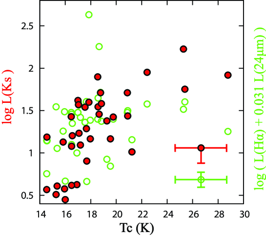
Figure 10: Relation between the cold dust temperature and $\mathrm{K_{S}}$ flux (Red circles) and ionizing flux (Green circles) estimated from a combination of H$\alpha$ and 24$\mu\mathrm{m}$ flux. The y-axis units are arbitrary shifted for comparison. The errorbar for the $\mathrm{K_{S}}$ flux shows that the flux is given only as an upper limit, considering the contribution of hot dust or nebular/molecular lines. A uniform uncertainty of 2 K is used for the cold dust temperature errorbar, which is the characteristic value in figure 9.

Table 1: M 33

Parameter	Value	Referencea
R.A. (J2000)	$1^{\mathrm{h}}33^{\mathrm{m}}50.9^{\mathrm{s}}$	NEDb
Dec.	$30^{\circ}39^{\prime}36^{\prime\prime}$	NED
Inclination	$51^{\circ}$	(1)
Position Angle	$22^{\circ}$	(2)
Morphology	SA(s)cd	(3)
Optical Size	$70.8^{\prime}\times 41.7^{\prime}$	NED
Distance	$840\$ kpc	(4)
$\mathrm{M_{B}}$c	$-19.38\$mag.	(5)

Notes ^a : (1) Deul & van der Hulst (1987), (2) Regan & Vogel (1994), (3) The Third Reference Catalogue of Bright Galaxies (RC3;de Vaucouleurs et al. (1991)), (4) Freedman et al. (1991), (5) The HyperLEDA database, Paturel et al. (2003). ^b : NASA Extragalactic Database. ^c : Absolute B band magnitude.

Table 2: Test sources ^a

R.A.	Dec.	FWHM	Peak Intensity	Total Flux
J2000	J2000	′′	$\mathrm{mJy\ beam^{-1}}$	Jy
$01^{\mathrm{h}}33^{\mathrm{m}}31.9^{\mathrm{s}}$	$+30^{\circ}56^{\prime}16.8^{\prime\prime}$	$60.0$	10.0	0.058
		$59.7$	9.6	0.055
$01^{\mathrm{h}}33^{\mathrm{m}}46.3^{\mathrm{s}}$	$+30^{\circ}59^{\prime}48.1^{\prime\prime}$	$60.0$	15	0.087
		$49.5$	15.9	0.062
$01^{\mathrm{h}}34^{\mathrm{m}}10.9^{\mathrm{s}}$	$+30^{\circ}58^{\prime}54.9^{\prime\prime}$	$120$	15.0	0.35
		$102$	12.7	0.21
$01^{\mathrm{h}}34^{\mathrm{m}}55.9^{\mathrm{s}}$	$+30^{\circ}58^{\prime}42.8^{\prime\prime}$	$120$	25.0	0.58
		$110$	22.1	0.43
$01^{\mathrm{h}}34^{\mathrm{m}}55.7^{\mathrm{s}}$	$+30^{\circ}50^{\prime}11.1^{\prime\prime}$	$180$	45	2.3
		$157$	36.2	1.4

Notes ^a : The lower row for each source corresponds to parameters obtained after reduction using the FRUIT algorithm. The reduced data were fitted with two dimensional gaussian, centered at the position were it was embedded.

Table 3: Flux Density at Various Wavelengths.

Wavelength	Flux	Referencea
$\ \mu\mathrm{m}$	$\log\mathrm{Jy}$
24	1.70	(1)
60	2.75	(2)
70	2.82	(1)
100	3.10	(2)
160	3.31	(1)
170	3.34	(2)
1100	1.00	This work

Notes ^a : (1): Hinz et al. (2004). (2):Hippelein et al. (2003).

References

- Alton et al. (2002) Alton, P. B., Bianchi, S., Richer, J., Pierce-Price, D., & Combes, F. 2002, A&A, 388, 446
- Bendo et al. (2010) Bendo, G. J., et al. 2010, A&A, 518, L65
- Bianchi et al. (2000) Bianchi, S., Davies, J. I., & Alton, P. B. 2000, A&A, 359, 65
- Buckalew et al. (2005) Buckalew, B. A., Kobulnicky, H. A., & Dufour, R. J. 2005, ApJS, 157, 30
- Calzetti et al. (2007) Calzetti, D., et al. 2007, ApJ, 666, 870
- Chini & Kruegel (1993) Chini, R., & Kruegel, E. 1993, A&A, 279, 385
- Chini et al. (1995) Chini, R., Kruegel, E., Lemke, R., & Ward-Thompson, D. 1995, A&A, 295, 317
- Crockett et al. (2006) Crockett, N. R., Garnett, D. R., Massey, P., & Jacoby, G. 2006, ApJ, 637, 741
- Dale & Helou (2002) Dale, D. A., & Helou, G. 2002, ApJ, 576, 159
- Davies et al. (1999) Davies, J. I., Alton, P., Trewhella, M., Evans, R., & Bianchi, S. 1999, MNRAS, 304, 495
- Deul & van der Hulst (1987) Deul, E. R., & van der Hulst, J. M. 1987, A&AS, 67, 509
- Devereux & Young (1990) Devereux, N. A., & Young, J. S. 1990, ApJ, 359, 42
- Devereux et al. (1997) Devereux, N., Duric, N., & Scowen, P. A. 1997, AJ, 113, 236
- Devost (1999) Devost, D. 1999, AJ, 118, 549
- Draine & Lee (1984) Draine, B. T., & Lee, H. M. 1984, ApJ, 285, 89
- Dumke et al. (2004) Dumke, M., Krause, M., & Wielebinski, R. 2004, A&A, 414, 475
- Dunne et al. (2000) Dunne, L., Eales, S., Edmunds, M., Ivison, R., Alexander, P., & Clements, D. L. 2000, MNRAS, 315, 115
- Dunne & Eales (2001) Dunne, L., & Eales, S. A. 2001, MNRAS, 327, 697
- Enoch et al. (2006) Enoch, M. L., et al. 2006, ApJ, 638, 293
- Ezawa et al. (2004) Ezawa, H., Kawabe, R., Kohno, K., & Yamamoto, S. 2004, Proc. SPIE, 5489, 763
- Ezawa et al. (2008) Ezawa, H., et al. 2008, Proc. SPIE, 7012
- Freedman et al. (1991) Freedman, W. L., Wilson, C. D., & Madore, B. F. 1991, ApJ, 372, 455
- Galliano et al. (2003) Galliano, F., Madden, S. C., Jones, A. P., Wilson, C. D., Bernard, J.-P., & Le Peintre, F. 2003, A&A, 407, 159
- Gordon (1988) Gordon, M. A. 1988, ApJ, 331, 509
- Griffin & Orton (1993) Griffin, M. J., & Orton, G. S. 1993, Icarus, 105, 537
- Heyer et al. (2004) Heyer, M. H., Corbelli, E., Schneider, S. E., & Young, J. S. 2004, ApJ, 602, 723
- Hill et al. (2006) Hill, T., Thompson, M. A., Burton, M. G., Walsh, A. J., Minier, V., Cunningham, M. R., & Pierce-Price, D. 2006, MNRAS, 368, 1223
- Hinz et al. (2004) Hinz, J. L., et al. 2004, ApJS, 154, 259
- Hippelein et al. (2003) Hippelein, H., Haas, M., Tuffs, R. J., Lemke, D., Stickel, M., Klaas, U., Völk, H. J. 2003, A&A, 407, 137
- Högbom (1974) Högbom, J. A. 1974, A&AS, 15, 417
- Hoopes & Walterbos (2000) Hoopes, C. G., & Walterbos, R. A. M. 2000, ApJ, 541, 597
- Hunt et al. (2003) Hunt, L. K., Thuan, T. X., & Izotov, Y. I. 2003, ApJ, 588, 281
- Kamazaki et al. (2005) Kamazaki, T., et al. 2005, Astronomical Society of the Pacific Conference Series, 347, 533
- Knacke & Thomson (1973) Knacke, R. F., & Thomson, R. K. 1973, PASP, 85, 341
- Knapp et al. (1993) Knapp, G. R., Sandell, G., & Robson, E. I. 1993, ApJS, 88, 173
- Kohno (2005) Kohno, K. 2005, ASP Conf. Ser. 344: The Cool Universe: Observing Cosmic Dawn, 344, 242
- Kramer et al. (2010) Kramer, C., et al. 2010, A&A, 518, L67
- Kruegel & Siebenmorgen (1994) Kruegel, E., & Siebenmorgen, R. 1994, A&A, 288, 929
- Li & Draine (2001) Li, A., & Draine, B. T. 2001, ApJ, 554, 778
- Lis & Menten (1998) Lis, D. C., & Menten, K. M. 1998, ApJ, 507, 794
- Liu et al. (2010) Liu, G., et al. 2010, AJ, 139, 1190
- Magrini et al. (2007) Magrini, L., Vílchez, J. M.,Mampaso, A., Corradi, R. L. M., & Leisy, P. 2007, A&A, 470, 865
- Makovoz & Khan (2005) Makovoz, D., & Khan, I. 2005, Astronomical Data Analysis Software and Systems XIV, 347, 81
- Mathis & Whiffen (1989) Mathis, J. S., & Whiffen, G. 1989, ApJ, 341, 808
- Meijerink et al. (2005) Meijerink, R., Tilanus, R. P. J., Dullemond, C. P., Israel, F. P., & van der Werf, P. P. 2005, A&A, 430, 427
- Newton (1980) Newton, K. 1980, MNRAS, 190, 689
- Onodera et al. (2010) Onodera, S., et al. 2010, ApJ, 722, L127
- Ossenkopf & Henning (1994) Ossenkopf, V., & Henning, T. 1994, A&A, 291, 943
- Paturel et al. (2003) Paturel, G., Petit, C., Prugniel, P., Theureau, G., Rousseau, J., Brouty, M., Dubois, P., & Cambrésy, L. 2003, A&A, 412, 45
- Reach et al. (1995) Reach, W. T., et al. 1995, ApJ, 451, 188
- Regan & Vogel (1994) Regan, M. W., & Vogel, S. N. 1994, ApJ, 434, 536
- Rieke et al. (2004) Rieke, G. H., et al. 2004, ApJS, 154, 25
- Rosolowsky & Simon (2008) Rosolowsky, E., & Simon, J. D. 2008, ApJ, 675, 1213
- Scott et al. (2008) Scott, K. S., et al. 2008, MNRAS, 385, 2225
- Shimajiri et al. (2011) Shimajiri, Y., et al. 2011, PASJ, 63, 105
- Tabatabaei et al. (2007a) Tabatabaei, F. S., et al. 2007, A&A, 466, 509
- Tabatabaei et al. (2007b) Tabatabaei, F. S., Krause, M., & Beck, R. 2007, A&A, 472, 785
- Tabatabaei et al. (2007c) Tabatabaei, F. S., Beck, R., Krügel, E., Krause, M., Berkhuijsen, E. M., Gordon, K. D., & Menten, K. M. 2007, A&A, 475, 133
- de Vaucouleurs et al. (1991) de Vaucouleurs, G., de Vaucouleurs, A., Corwin, H. G., Jr., Buta, R. J., Paturel, G., & Fouque, P. 1991, Volume 1-3, XII, 2069 pp. 7 figs.. Springer-Verlag Berlin Heidelberg New York
- Verley et al. (2007) Verley, S., Hunt, L. K., Corbelli, E., & Giovanardi, C. 2007, A&A, 476, 1161
- Verley et al. (2009) Verley, S., Corbelli, E., Giovanardi, C., & Hunt, L. K. 2009, A&A, 493, 453
- Verley et al. (2010) Verley, S., et al. 2010, arXiv:1005.2297
- Vilchez et al. (1988) Vilchez,J. M., Pagel,B. E. J.,Diaz, A. I.,Terlevich, E., & Edmunds, M. G. 1988, MNRAS, 235, 633
- Weintraub et al. (1989) Weintraub, D. A., Sandell, G., & Duncan, W. D. 1989, ApJ, 340, L69
- Weiß et al. (2008) Weiß, A., Kovács, A., Güsten, R., Menten, K. M., Schuller, F., Siringo, G., & Kreysa, E. 2008, A&A, 490, 77
- Werner et al. (2004) Werner, M. W., et al. 2004, ApJS, 154, 1
- Williams et al. (2004) Williams, S. J., Fuller, G. A., & Sridharan, T. K. 2004, A&A, 417, 115
- Wilson et al. (2008) Wilson, G. W., et al. 2008, MNRAS, 386, 807
- Xu & Helou (1996) Xu, C., & Helou, G. 1996, ApJ, 456, 163