Splash singularity for water waves

Splash singularity for water waves

Abstract

We exhibit smooth initial data for the 2D water wave equation for which we prove that smoothness of the interface breaks down in finite time. Moreover, we show a stability result together with numerical evidence that there exist solutions of the 2D water wave equation that start from a graph, turn over and collapse in a splash singularity (self intersecting curve in one point) in finite time.

Keywords: Euler, incompressible, blow-up, water waves, splash.

1 Introduction

We consider the 2D water wave equation, which governs the motion of the interface between a 2D inviscid incompressible irrotational fluid and a vacuum, taking gravity into account but neglecting surface tension. We prove that an initially smooth interface may in finite time become singular by the mechanism illustrated in fig. 1. We call such a singularity a “splash”. We also present numerical evidence for a scenario in which the interface starts out as a smooth graph, then “turns over” after finite time, and finally produces a splash, as in fig. 4.

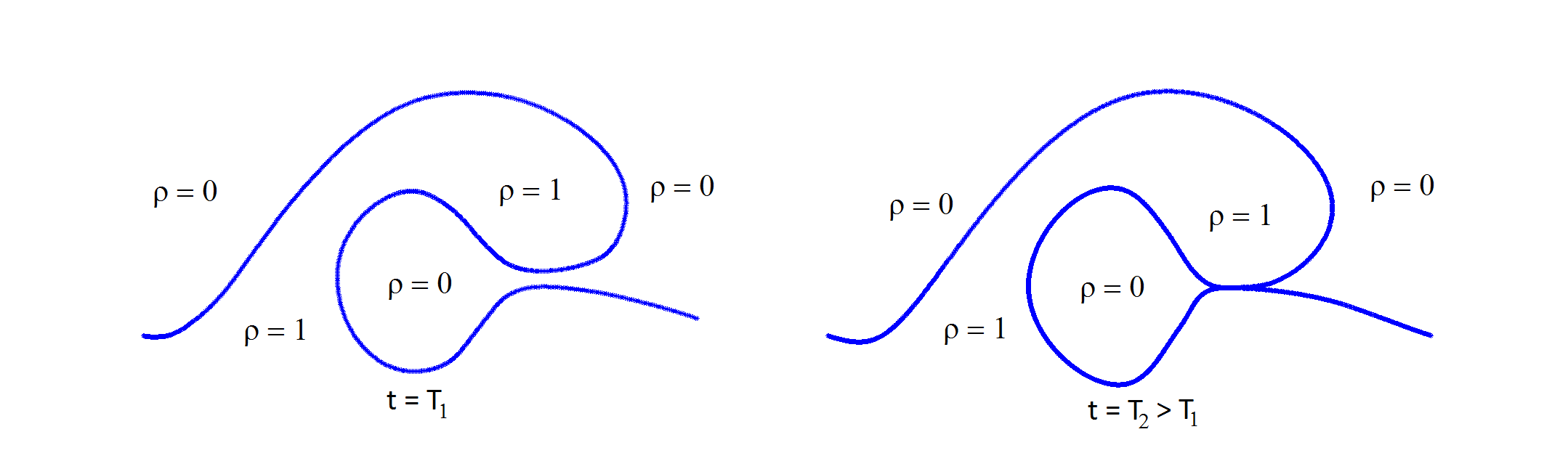
Figure 1: Splash singularity. The interface collapses at one point.

The equations of motion in $\mathbb{R}^{2}$ for the density $\rho=\rho(x,t)$, $x\in\mathbb{R}^{2}$, $t\geq 0$, the velocity $v=(v^{1},v^{2})$ and the pressure $p=p(x,t)$ are:

$$\left\{\begin{array}[]{ccc}\rho(v_{t}+v\cdot\nabla v)&=&-\nabla p-(0,\rho),\\ \rho_{t}+v\cdot\nabla\rho&=&0,\\ \nabla\cdot v&=&0.\end{array}\right.$$ (1)

Above, the acceleration due to gravity is taken equal to one for the sake of simplicity.

The free boundary is parameterized by

$$\partial\Omega^{j}(t)=\{z(\alpha,t)=(z_{1}(\alpha,t),z_{2}(\alpha,t)):\alpha\in\mathbb{R}\},$$

where the regions $\Omega^{j}(t)$ are defined by

$$\rho(x_{1},x_{2},t)=\left\{\begin{array}[]{cl}0,&x\in\Omega^{1}(t)\\ 1,&x\in\Omega^{2}(t)=\mathbb{R}^{2}-\Omega^{1}(t).\end{array}\right.$$

We assume that the fluid is irrotational, i.e. the vorticity $\nabla^{\bot}\cdot v=0$, in the interior of each domain $\Omega^{j}$ ($j=1,2$). The vorticity will be supported on the free boundary curve $z(\alpha,t)$ and it has the form

$$\nabla^{\bot}\cdot v(x,t)=\omega(\alpha,t)\delta(x-z(\alpha,t)),$$

i.e. the vorticity is a Dirac measure defined by

$$\langle\nabla^{\bot}\cdot v,\eta\rangle=\int_{\mathbb{R}}\omega(\alpha,t)\eta(z(\alpha,t))d\alpha,$$

with $\eta(x)$ a test function. We present results for the following geometries:

1. open curves asymptotic to the horizontal at infinity

   $$\lim_{\alpha\rightarrow\infty}(z(\alpha,t)-(\alpha,0))=0.$$

2. periodic curves in the space variable

   $$z(\alpha+2k\pi,t)=z(\alpha,t)+2k\pi(1,0).$$

3. closed contours

   $$z(\alpha+2k\pi,t)=z(\alpha,t).$$

However, in this paper we will only deal with the first case as the others are similar. One method to derive the equations for the evolution of $v$, $\rho$ is to write the velocity as the orthogonal gradient of the stream function, take the curl and recover the velocity by inverting the Laplacian, i.e., we apply the Biot-Savart law. Here we use the fact that the vorticity is concentrated on the interface;

$$v(x,t)=\nabla^{\bot}\Delta^{-1}(\nabla^{\bot}\cdot v)(x,t)=\frac{1}{2\pi}\int_{\mathbb{R}}\frac{(x-z(\alpha,t))^{\bot}}{|x-z(\alpha,t)|^{2}}\omega(\alpha,t)d\alpha,$$

with $x\neq z(\alpha,t)$.

Taking limits of the above equation, by approaching the boundary in the normal direction, we obtain the velocity of the interface, to which we can add any term $c$ in the tangential direction $z_{\alpha}$ without modifying the geometry of the interface. Thus the interface satisfies

$$z_{t}(\alpha,t)=BR(z,\omega)(\alpha,t)+c(\alpha,t)z_{\alpha}(\alpha,t),$$ (2)

where the Birkhoff-Rott integral is defined by

$$BR(z,\omega)=\frac{1}{2\pi}P.V.\int_{\mathbb{R}}\frac{(z(\alpha,t)-z(\beta,t))^{\bot}}{|z(\alpha,t)-z(\beta,t)|^{2}}\omega(\alpha,t)d\alpha.$$

The system is closed by using Euler equations (for details see for example [9]);

$$\begin{split}\omega_{t}(\alpha,t)&=-2\partial_{t}BR(z,\omega)(\alpha,t)\cdot\partial_{\alpha}z(\alpha,t)-\partial_{\alpha}(\frac{|\omega|^{2}}{4|\partial_{\alpha}z|^{2}})(\alpha,t)+\partial_{\alpha}(c\omega)(\alpha,t)\\ &\quad+2c(\alpha,t)\partial_{\alpha}BR(z,\omega)(\alpha,t)\cdot\partial_{\alpha}z(\alpha,t)+2\partial_{\alpha}z_{2}(\alpha,t).\end{split}$$ (3)

Then the dynamic equations, for the interface $z=z(\alpha,t)$ and the vorticity are the system given by (2) and (3) and are known as the water-wave equations.

Taking the divergence of the Euler equation (1) and recalling that the flow is irrotational in the interior of the regions $\Omega^{j}(t)$, we find that

$$-\Delta p=|\nabla v|^{2}\geq 0$$

which, together with the fact that the pressure is zero on the interface implies by Hopf’s lemma in $\Omega^{2}(t)$ that

$$\sigma(\alpha,t)\equiv-|z_{\alpha}^{\perp}(\alpha,t)|\partial_{n}p(z(\alpha,t),t)>0,$$

where $\partial_{n}$ denotes the normal derivative. This is known as the Rayleigh-Taylor condition (see [20] and [22]) which was first proved by Wu in [23] and [24].

The first results concerning the Cauchy problem for the linearized version of water waves and small data in Sobolev spaces are due to Craig [11], Nalimov [17], Beale et al. [5] and Yoshihara [27]. The well-posedness in Sobolev spaces for the water-wave problem was proven by Wu in [23] with the assumption that the initial free interface is non-self-intersecting (satisfies the arc-chord condition). For recent work on local existence see Wu [24], Christodoulou-Lindblad [8], Lindblad [15], Coutand-Shkoller [10], Shatah-Zeng [21], Zhang-Zhang [28], Córdoba et al. [9], Lannes [13], [14], Alazard-Metivier [1] and Ambrose-Masmoudi [3]. The issue of long time existence has been treated in Alvarez-Lannes [2] where well-posedness over large time scales is shown and different asymptotic regimes are justified. Wu proved in [25] exponential time of existence in two dimensions for small initial data, and Germain et al. in [12] and Wu in [26] global existence for small data in the three dimensional case (two dimensional interface). In [6] and [7], Castro et al. showed that there exist large initial data parameterized as a graph for which in finite time the interface reaches a regime in which it is no longer a graph. For previous numerical simulations showing this phenomenon see Beale et al. [4].

The outline of the paper is the following: in section 2 we will describe the equations in a transformed domain which will circumvent the problem of having a singularity where the arc-chord condition fails as the curve self-intersects, i.e. a splash singularity forms. In section 3 we will outline the proof of a local existence theorem for the equations in the new domain, both for the analytic case and for Sobolev spaces. Section 4 will be devoted to a stability theorem, whereas section 5 will comment on the numerical results obtained towards the splash singularity starting from a graph. Finally in section 6 we describe the ideas that we hope will lead to a computer assisted proof of the existence of a solution that starts as a graph and ends in a splash.

2 The equations in the tilde domain

In this section we will rewrite the equations by applying a transformation from the original coordinates to new ones which we will denote with a tilde. The purpose of this transformation is to be able to deal with the failure of the arc-chord condition. We start by reformulating the set of equations, in the non tilde domain, for the case of a periodic contour in terms of the velocity potential. From (1) and since $v$ is irrotational in $\Omega^{2}(t)$ we have that:

$$\nabla\times v =0\quad\text{in $\Omega^{2}(t)$}$$

$$\nabla\cdot v =0\quad\text{in $\Omega^{2}(t)$}$$

$$\phi_{t}(x,y,t)+\frac{1}{2}|v(x,y,t)|^{2} =-(p(x,y,t)-p^{*}(t))-y\quad\text{in $\Omega^{2}(t)$}$$

$$z_{t}(\alpha,t) =u(\alpha,t)+c(\alpha,t)z_{\alpha}(\alpha,t)$$

$$\Phi_{\alpha}(\alpha,t) =u(\alpha,t)\cdot z_{\alpha}(\alpha,t)$$

$$p =\text{constant}\equiv 0\quad\text{in $\Omega^{1}(t)$}$$

$$z(\alpha,0) =z^{0}(\alpha)$$

$$\Phi_{\alpha}(\alpha,0) =\Phi_{\alpha}^{0}(\alpha)$$ (4)

where $\phi$ is the velocity potential, $\Phi(\alpha,t)$ is its limit at the interface coming from the fluid region, $\nabla\phi=v$, $p^{*}$ is a function of $t$ alone, $c$ is a free quantity which represents the reparameterization freedom, $u(\alpha,t)$ is the limit of the velocity at the interface coming from the fluid region and $\Phi_{\alpha}^{0}(\alpha)$ has zero mean. We also want the velocity to be in $L^{2}\left(\Omega^{2}(t)\cap\left([-\pi,\pi]\times\mathbb{R}\right)\right)$ and periodic in the $x-$coordinate i.e.

$$v(x+2\pi,y)=v(x,y)\quad\text{in $\Omega^{2}(t)$}.$$

Note that $\Phi$ is periodic in the horizontal variable, because $v$ is periodic and $v(x,y)$ tends to zero as $y$ tends to $-\infty$.

In order to simplify this system we use the stream function $\psi$ and consider the equations

$$\Delta\psi(x,y,t) =0\quad\text{in $\Omega^{2}(t)$}$$

$$\left.\partial_{n}\psi\right|_{z(\alpha,t)} =-\frac{\Phi_{\alpha}(\alpha,t)}{|z_{\alpha}(\alpha,t)|}$$

$$\psi(x+2\pi,y,t) =\psi(x,y,t)\quad\text{in $\Omega^{2}(t)$}$$

$$\psi(x,y) O(1) y\to-\infty$$ is as

$$v \equiv\nabla^{\perp}\psi\quad\text{in $\Omega^{2}(t)$}$$

$$z_{t}(\alpha,t) =u(\alpha,t)+c(\alpha,t)z_{\alpha}(\alpha,t)$$

$$\phi(x,y,t) \psi(x,y,t) \Omega^{2}$$ is the harmonic conjugate of in

$$\Phi_{t}(\alpha,t) =\frac{1}{2}|u(\alpha,t)|^{2}+c(\alpha,t)u(\alpha,t)\cdot z_{\alpha}(\alpha,t)-z_{2}(\alpha,t)+p^{*}(t)$$

$$z(\alpha,0) =z^{0}(\alpha)$$

$$\Phi_{\alpha}(\alpha,0) =\Phi_{\alpha}^{0}(\alpha)$$ (5)

Although we may take as an initial condition the tangential component of the velocity multiplied by the modulus of the tangent vector, i.e. $\Phi_{\alpha}$, we can also solve the system (2) by taking as an initial condition the normal component of the initial velocity multiplied by the modulus of the normal vector, i.e. $\Psi_{\alpha}$, ($\Psi(\alpha,t)=\psi(z(\alpha,t),t)$), as we can transform one into the other.

It can be checked that solutions of the system (2) are also solutions of the system (2). Let us consider $\tilde{z}(\alpha,t)=(\tilde{z}_{1}(\alpha,t),\tilde{z}_{2}(\alpha,t))\equiv P(z(\alpha,t))$ where $P$ is a conformal map defined in the water region that will be given as:

$$P(w)=\left(\tan\left(\frac{w}{2}\right)\right)^{1/2},\quad w\in\mathbb{C},$$

for a branch of the square root that separates the self-intersecting points of the interface. Here $P(w)$ will refer to a 2 dimensional vector whose components are the real and imaginary parts of $P(w_{1}+iw_{2})$. In this setting, $P^{-1}(z)$ will be well defined modulo multiples of $2\pi$.

The water wave equations are invariant under time reversal. To obtain a solution that ends in a splash, we can therefore take our initial condition to be a splash, and show that there is a smooth solution for small times $t>0$. As initial data we are interested in considering a curve that intersects itself at one point, as in fig. 4. More precisely, we will use as initial data splash curves which are defined as follows:

Definition 2.1

We say that $z(\alpha)$ is a splash curve if

1. $z_{1}(\alpha)-\alpha,z_{2}(\alpha)$ are smooth functions and $2\pi$-periodic.

2. $z(\alpha)$ satisfies the arc-chord condition at every point except at $\alpha_{1}$ and $\alpha_{2}$, with $\alpha_{1}<\alpha_{2}$ where $z(\alpha_{1})=z(\alpha_{2})$ and $|z_{\alpha}(\alpha_{1})|,|z_{\alpha}(\alpha_{2})|>0$. This means $z(\alpha_{1})=z(\alpha_{2})$, but if we remove either a neighborhood of $\alpha_{1}$ or a neighborhood of $\alpha_{2}$ in parameter space, then the arc-chord condition holds.

3. The curve $z(\alpha)$ separates the complex plane into two region; a connected water region and a vacuum region. The water region contains each point $x+iy$ for which y is large negative. We choose the parametrization such that the normal vector $n=\frac{(-\partial_{\alpha}z^{2}(\alpha),\partial_{\alpha}z^{1}(\alpha))}{|\partial_{\alpha}z(\alpha)|}$ points to the vacuum region.

4. We can choose a branch of the function $P$ on the water region such that the curve $\tilde{z}(\alpha)=P(z(\alpha))$ satisfies:

   1. $\tilde{z}_{1}(\alpha)$ and $\tilde{z}_{2}(\alpha)$ are smooth and $2\pi$-periodic.

   2. $\tilde{z}$ is a closed contour.

   3. $\tilde{z}$ satisfies the arc-chord condition.

   We will choose the branch of the root that produces that

   $$\lim_{y\to-\infty}P(x+iy)=-e^{-i\pi/4}$$

   independently of $x$.

5. $P(w)$ is analytic in $w$ and $\frac{dP}{dw}(w)\neq 0$ if $w$ belongs to the water region.

6. $\tilde{z}(\alpha)\neq q^{l}$ for $l=0,...,4$, where

   $$q^{0}=\left(0,0\right),\quad q^{1}=\left(\frac{1}{\sqrt{2}},\frac{1}{\sqrt{2}}\right),\quad q^{2}=\left(\frac{-1}{\sqrt{2}},\frac{1}{\sqrt{2}}\right),\quad q^{3}=\left(\frac{-1}{\sqrt{2}},\frac{-1}{\sqrt{2}}\right),\quad q^{4}=\left(\frac{1}{\sqrt{2}},\frac{-1}{\sqrt{2}}\right).$$ (6)

From now on, we will always work with splash curves as initial data. Condition 6 will be used in the local existence theorems and can be proved to hold for short enough time as long as the initial condition satisfies it. We will also need that the interface passes below the points $(\pm\pi,0)$ (or, equivalently, that those points belong to the vacuum region) in order for the tilde region to be a closed curve and the vacuum region to lie on the outer part. For a splash curve this is trivial from the definition. For more information about the transformation of both regions, check the figures 4 and 4 and notice that we rule out the scenarios in fig. 2.

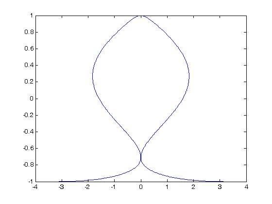
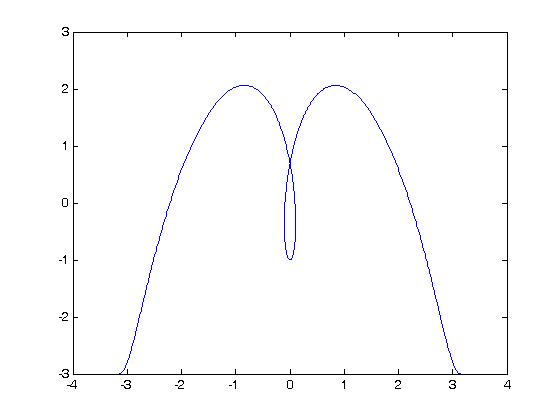
Figure 2: Two examples of non-splash curves.

We will now write (2) in the new tilde coordinates. We define the following quantities:

$$\tilde{\psi}(x,y,t)\equiv\psi(P^{-1}(x,y,t)),\quad\tilde{\phi}(x,y,t)\equiv\phi(P^{-1}(x,y,t)),\quad\tilde{v}(x,y,t)\equiv\nabla\tilde{\phi}(x,y,t).$$

Let us note that as $\psi$ and $\phi$ are $2\pi$ periodic, the resulting $\tilde{\psi}$ and $\tilde{\phi}$ are well defined. We do not have problems with the harmonicity of $\tilde{\psi}$ or $\tilde{\phi}$ at the point which is mapped from minus infinity (which belongs to the water region) by $P$ as $\phi$ and $\psi$ are well defined at infinity. Also, the periodicity of $\phi$ and $\psi$ causes $\tilde{\phi}$ and $\tilde{\psi}$ to be continuous (and harmonic) at the interior of $P(\Omega^{2}(t))$.

Let us assume that there exists a solution of (2) and that we take $u_{n}=\frac{\Psi_{\alpha}}{|z_{\alpha}|}$ such that $u_{n}(\alpha_{1}),u_{n}(\alpha_{2})<0$ for all $0<t<T,T$ small enough, thus $z(\alpha,t)$ satisfies the arc-chord condition and does not touch the removed branch from $P(w)$.

Thus the system (2) in the new coordinates reads

$$\Delta\tilde{\psi}(x,y,t) =0\quad\text{in $P(\Omega^{2}(t))$}$$

$$\left.\partial_{n}\tilde{\psi}\right|_{\tilde{z}(\alpha,t)} =-\frac{\tilde{\Phi}_{\alpha}(\alpha,t)}{|\tilde{z}_{\alpha}(\alpha,t)|}$$

$$\tilde{v} \equiv\nabla^{\perp}\tilde{\psi}\quad\text{in $P(\Omega^{2}(t))$}$$

$$\tilde{z}_{t}(\alpha,t) =Q^{2}(\alpha,t)\tilde{u}(\alpha,t)+c(\alpha,t)\tilde{z}_{\alpha}(\alpha,t)$$

$$\tilde{\Phi}_{t}(\alpha,t) =\frac{1}{2}Q^{2}(\alpha,t)|\tilde{u}(\alpha,t)|^{2}+c(\alpha,t)\tilde{u}(\alpha,t)\cdot\tilde{z}_{\alpha}(\alpha,t)-P^{-1}_{2}(\tilde{z}(\alpha,t))+p^{*}(t)$$

$$\tilde{z}(\alpha,0) =\tilde{z}^{0}(\alpha)$$

$$\tilde{\Phi}_{\alpha}(\alpha,0) =\tilde{\Phi}_{\alpha}^{0}(\alpha)=\Phi_{\alpha}^{0}(\alpha).$$ (7)

where $\tilde{u}$ is the limit of the velocity coming from the fluid region in the tilde domain and $Q^{2}(\alpha,t)=\left|\frac{dP}{dw}(z(\alpha,t))\right|^{2}$.

We can therefore solve the Neumann problem for the stream function in the fluid domain with boundary conditions on the interface. In fact there exists a function $\tilde{\omega}$ satisfying

$$\psi(\tilde{x},t)=\frac{1}{2\pi}\int_{-\pi}^{\pi}\log(|\tilde{x}-\tilde{z}(\alpha,t)|)\tilde{\omega}(\alpha,t)d\alpha,\quad\tilde{x}\text{ belonging to the fluid region, }$$

which implies

$$\tilde{v}(\tilde{x},t)=\nabla^{\perp}\tilde{\psi}(\tilde{x},t)=\frac{1}{2\pi}P.V\int_{-\pi}^{\pi}\frac{(\tilde{x}-\tilde{z}(\alpha,t))^{\perp}}{|\tilde{x}-\tilde{z}(\alpha,t)|^{2}}\tilde{\omega}(\alpha,t)d\alpha.$$

Taking limits from the fluid region we obtain

$$\tilde{u}(\alpha,t)=BR(\tilde{z},\tilde{\omega})+\frac{\tilde{\omega}}{2|\tilde{z}_{\alpha}|^{2}}\tilde{z}_{\alpha}.$$

The evolution of $\tilde{\omega}$ is calculated in the following way. First, let us recall the equations

$$\tilde{z}_{t}(\alpha,t) =Q^{2}(\alpha,t)\tilde{u}(\alpha,t)+c(\alpha,t)\tilde{z}_{\alpha}(\alpha,t)$$

$$\tilde{\Phi}_{t}(\alpha,t) =\frac{1}{2}Q^{2}(\alpha,t)|\tilde{u}(\alpha,t)|^{2}+c(\alpha,t)\tilde{u}(\alpha,t)\cdot\tilde{z}_{\alpha}(\alpha,t)-P^{-1}_{2}(\tilde{z}(\alpha,t))$$

$$\tilde{\Phi}_{\alpha}(\alpha,t) =\tilde{u}(\alpha,t)\cdot\tilde{z}_{\alpha}(\alpha,t)$$

$$\tilde{z}(\alpha,0) =\tilde{z}^{0}(\alpha)$$

$$\tilde{\Phi}_{\alpha}(\alpha,0) =\tilde{\Phi}_{\alpha}^{0}(\alpha)=\Phi_{\alpha}^{0}(\alpha)$$ (8)

Those equations will be the ones used in section 5 with $c(\alpha,t)=0$. Substituting the expression for $\tilde{u}(\alpha,t)$ and performing the change $\tilde{c}(\alpha,t)=c(\alpha,t)+\frac{1}{2}Q^{2}(\alpha,t)\frac{\tilde{\omega}(\alpha,t)}{|\tilde{z}_{\alpha}(\alpha,t)|^{2}}$ we obtain

$$\tilde{z}_{t}(\alpha,t) =Q^{2}(\alpha,t)BR(\tilde{z},\tilde{\omega})(\alpha,t)+\tilde{c}(\alpha,t)\tilde{z}_{\alpha}(\alpha,t)$$ (9)

and the evolution equation for $\tilde{\omega}$

$$\tilde{\omega}_{t}(\alpha,t) =-2\partial_{t}BR(\tilde{z},\tilde{\omega})(\alpha,t)\cdot\tilde{z}_{\alpha}(\alpha,t)-|BR(\tilde{z},\tilde{\omega})|^{2}\partial_{\alpha}Q^{2}(\alpha,t)$$

$$-\partial_{\alpha}\left(\frac{Q^{2}(\alpha,t)}{4}\frac{\tilde{\omega}(\alpha,t)^{2}}{|\tilde{z}_{\alpha}(\alpha,t)|^{2}}\right)+2\tilde{c}(\alpha,t)\partial_{\alpha}BR(\tilde{z},\tilde{\omega})\cdot\tilde{z}_{\alpha}(\alpha,t)$$

$$+\partial_{\alpha}\left(\tilde{c}(\alpha,t)\tilde{\omega}(\alpha,t)\right)-2\partial_{\alpha}\left(P^{-1}_{2}(\tilde{z}(\alpha,t))\right).$$ (10)

Remark 2.2

Equation (2) is analogous to (3). In fact, if we set $Q\equiv 1$ in (2) we recover (3).

Note that for the tilde domain, the Rayleigh-Taylor condition is the same as in the first domain, i.e:

$$\nabla p(\alpha,t)\cdot z_{\alpha}^{\perp}(\alpha,t)=\nabla\tilde{p}(\alpha,t)\cdot\tilde{z}_{\alpha}^{\perp}(\alpha,t)$$

where $\tilde{p}=p\circ P^{-1}$.

Our strategy will be the following: we will consider the evolution of the solutions in the tilde domain and then see that everything works fine in the original domain.

We will have to obtain the normal velocity once given the tangential velocity, and viceversa. To do this, we just have to notice that

$$\tilde{\Phi}_{\alpha}(\alpha,t)=\tilde{u}(\alpha,t)\cdot\tilde{z}_{\alpha}(\alpha,t)=BR(\tilde{z},\tilde{\omega})\cdot\tilde{z}_{\alpha}(\alpha,t)+\frac{\tilde{\omega}(\alpha,t)}{2}.$$

From that, we can invert the equation and get $\tilde{\omega}$, plug it into the following expression for $\tilde{\psi}$:

$$\tilde{\psi}(\tilde{x})=\frac{1}{2\pi}\int_{-\pi}^{\pi}\log(|\tilde{x}-\tilde{z}(\alpha)|)\tilde{\omega}(\alpha)d\alpha$$

and restrict ourselves to the interface to get $\tilde{\Psi}(\alpha,t)$. Taking a derivative in $\alpha$ we can recover the normal component of the velocity. An analogous reasoning can be done to get the tangential velocity from the normal by solving the complementary Neumann problem for $\phi$.

We now note that a solution of the system (2) in the tilde domain gives rise to a solution of the system (2) in the non-tilde domain, by inverting the map $P$. In fact, this will be the implication used in Theorem 3.1 (finding a solution in the tilde domain, and therefore in the non-tilde).

Remark 2.3

A similar argument works for the other two settings (closed contour and asymptotic to horizontal) by choosing an appropriate $P(w)$ that separates the singularity.

3 Local existence at the splash

The main result in this section is a local existence proof for the splash singularity. To avoid the arc-chord condition failure, we will prove the local existence in the tilde domain. This can be done in two different settings, namely in the space of analytic functions and the Sobolev space $H^{s}$.

Theorem 3.1

Let $z^{0}(\alpha)$ be a splash curve such that $z_{1}^{0}(\alpha)-\alpha,z_{2}^{0}(\alpha)\in H^{4}(\mathbb{T})$. Let $u^{0}(\alpha)\cdot(z^{0}_{\alpha})^{\perp}(\alpha)\in H^{4}(\mathbb{T})$ satisfying:

1. $\displaystyle\left(u^{0}\cdot\frac{(z_{\alpha}^{0})^{\bot}}{|z_{\alpha}^{0}|}\right)(\alpha_{1})<0,\left(u^{0}\cdot\frac{(z_{\alpha}^{0})^{\bot}}{|z_{\alpha}^{0}|}\right)(\alpha_{2})<0,$

2. $\displaystyle\int_{\partial\Omega}u^{0}\cdot\frac{(z_{\alpha}^{0})^{\bot}}{|z_{\alpha}^{0}|}ds=\int_{\mathbb{T}}u^{0}(\alpha)\cdot(z_{\alpha}^{0})^{\bot}d\alpha=0$.

Then there exist a finite time $T>0$, a time-varying curve $z(\alpha,t)\in C([0,T];H^{4}(\mathbb{T}))$ satisfying:

1. $z_{1}(\alpha,t)-\alpha,z_{2}(\alpha,t)$ are $2\pi$-periodic,

2. $z(\alpha,t)$ satisfies the arc-chord condition for all $t\in(0,T]$,

and $u(\alpha,t)\in C([0,T];H^{3}(\mathbb{T}))$ which provides a solution of the water wave equations (2) with $z(\alpha,0)=z^{0}(\alpha)$ and $u(\alpha,0)\cdot(z_{\alpha})^{\perp}(\alpha,0)=u^{0}(\alpha)\cdot(z^{0}_{\alpha})^{\perp}(\alpha)$.

Sketch of the proof: Using the fact that there is local existence to the initial data in the tilde domain and applying $P^{-1}$ to the solution obtained there, we can get a curve $z(\alpha,t)$ that solves the water waves equation in the non tilde domain. This leads to the proof of Theorem 3.1. Details on the local existence in the tilde domain are shown below.

3.1 Local existence for analytic initial data in the tilde domain

In this subsection, we will work on the tilde domain, and all tildes will be dropped for the sake of simplicity.

We will work with $c=0$. We have the following system:

$$\left\{\begin{array}[]{rcl}z_{t}&=&\left|\frac{dP}{dw}(P^{-1}(z))\right|^{2}u\\ \Phi_{t}&=&\frac{1}{2}\left|\frac{dP}{dw}(P^{-1}(z))\right|^{2}|u|^{2}-P_{2}^{-1}(z)\\ u&=&BR(z,\omega)+\frac{\omega}{2|z_{\alpha}|^{2}}z_{\alpha}\\ \Phi_{\alpha}&=&\frac{\omega}{2}+BR(z,\omega)\cdot z_{\alpha}\\ \left|\frac{dP}{dw}(P^{-1}(z(\alpha,t)))\right|^{2}&=&\frac{1}{16}\left|\frac{1+(z_{1}(\alpha,t)+iz_{2}(\alpha,t))^{4}}{z_{1}(\alpha,t)+iz_{2}(\alpha,t)}\right|^{2}\\ P_{2}^{-1}(z(\alpha,t))&=&\ln\left|\frac{i+(z_{1}(\alpha,t)+iz_{2}(\alpha,t))^{2}}{i-(z_{1}(\alpha,t)+iz_{2}(\alpha,t))^{2}}\right|\end{array}\right.$$ (11)

We demand that $z^{0}(\alpha)\neq(0,0)$ to find the function $\frac{dP}{dw}(P^{-1}(z(\alpha,t)))$ well defined. This condition is going to remain true for short time. We also consider $z^{0}(\alpha)\neq q^{l}$, $l=1,...,4$ in (6) to get $P_{2}^{-1}(z(\alpha,t))$ well defined. Again this is going to remain true for short time.

We consider the space

$$H^{3}(\partial S_{r})=\left\{f\right. \text{ analytic in }S_{r}=\{\alpha+i\eta,|\eta|<r\}:\,\|f\|_{r}^{2}<\infty$$

$$\|f\|_{r}^{2}=\|f\|^{2}_{L^{2}(\partial S_{r})}+\|\partial_{\alpha}^{3}f\|^{2}_{L^{2}(\partial S_{r})}\text{ where }$$

$$\left.\|f\|^{2}_{L^{2}(\partial S_{r})}=\sum_{\pm}\int_{-\pi}^{\pi}|f(\alpha\pm ir)|^{2}d\alpha,f\;2\pi\text{-periodic}\right\}$$

and $(z,\Phi)\in(H^{3}(\partial S_{r}))^{3}\equiv X_{r}$.

We have the following theorem:

Theorem 3.2

Let $z^{0}(\alpha)$ be a splash curve and let $u^{0}\cdot\frac{z^{0}_{\alpha}}{|z^{0}_{\alpha}|}(\alpha)=\frac{\Phi^{0}_{\alpha}}{|z^{0}_{\alpha}|}(\alpha)$ be the initial tangential velocity such that

$$(z_{1}^{0}(\alpha)-\alpha,z_{2}^{0},(\alpha),\Phi^{0}_{\alpha}(\alpha))\in X_{r_{0}},$$

for some $r_{0}>0$, and satisfying:

1. $\displaystyle\left(u^{0}\cdot\frac{(z_{\alpha}^{0})^{\bot}}{|z_{\alpha}^{0}|}\right)(\alpha_{1})<0,\left(u^{0}\cdot\frac{(z_{\alpha}^{0})^{\bot}}{|z_{\alpha}^{0}|}\right)(\alpha_{2})<0,$

2. $\displaystyle\int_{\partial\Omega}u^{0}\cdot\frac{(z_{\alpha}^{0})^{\bot}}{|z_{\alpha}^{0}|}ds=\int_{\mathbb{T}}u^{0}(\alpha)\cdot(z_{\alpha}^{0})^{\bot}d\alpha=0$.

Then there exist a finite time $T>0$, $0<r<r_{0}$, a time-varying curve $\tilde{z}(\alpha,t)$ satisfying:

1. $P^{-1}(\tilde{z}_{1}(\alpha,t))-\alpha,P^{-1}(\tilde{z}_{2}(\alpha,t))$ are $2\pi$-periodic,

2. $P^{-1}(\tilde{z}(\alpha,t))$ satisfies the arc-chord condition for all $t\in(0,T]$,

and $\tilde{u}(\alpha,t)$ with

$$(\tilde{z}_{1}(\alpha,t)-\alpha,\tilde{z}_{2}(\alpha,t),\tilde{\Phi}_{\alpha}(\alpha,t)(\alpha,t))\in C([0,T],X_{r})$$

which provides a solution of the water waves equations (11) with $\tilde{z}^{0}(\alpha)=P(z^{0}(\alpha))$ and $\tilde{u}(\alpha,0)\cdot(\tilde{z}_{\alpha})^{\perp}(\alpha,0)=u^{0}(\alpha)\cdot(\tilde{z}^{0})^{\perp}_{\alpha}(\alpha)$.

The main tool in the proof is to use an abstract Cauchy-Kowaleswki theorem from [18] and [19] as in for example [6].

3.2 Local existence for initial data in Sobolev spaces in the tilde domain

We will take the following $\tilde{c}(\alpha,t)$:

$$\tilde{c}(\alpha,t) =\frac{\alpha+\pi}{2\pi}\int_{-\pi}^{\pi}(Q^{2}BR(\tilde{z},\tilde{\omega}))_{\beta}(\beta,t)\cdot\frac{\tilde{z}_{\beta}(\beta,t)}{|\tilde{z}_{\beta}(\beta,t)|^{2}}d\beta$$

$$-\int_{-\pi}^{\alpha}(Q^{2}BR(\tilde{z},\tilde{\omega}))_{\beta}(\beta,t)\cdot\frac{\tilde{z}_{\beta}(\beta,t)}{|\tilde{z}_{\beta}(\beta,t)|^{2}}d\beta$$

We will also define an auxiliary function $\tilde{\varphi}(\alpha,t)$ analogous to the one introduced in [5] (for the linear case) and [3] (nonlinear case) which helps us to bound several of the terms that appear:

$$\tilde{\varphi}(\alpha,t)=\frac{Q^{2}(\alpha,t)\tilde{\omega}(\alpha,t)}{2|\tilde{z}_{\alpha}(\alpha,t)|}-\tilde{c}(\alpha,t)|\tilde{z}_{\alpha}(\alpha,t)|.$$ (12)

Theorem 3.3

Let $z^{0}(\alpha)$ be a splash curve such that $z_{1}^{0}(\alpha)-\alpha,z_{2}^{0}(\alpha)\in H^{4}(\mathbb{T})$. Let $u^{0}(\alpha)\cdot(z^{0}_{\alpha})^{\perp}(\alpha)\in H^{4}(\mathbb{T})$ satisfying:

1. $\displaystyle\left(u^{0}\cdot\frac{(z_{\alpha}^{0})^{\bot}}{|z_{\alpha}^{0}|}\right)(\alpha_{1})<0,\left(u^{0}\cdot\frac{(z_{\alpha}^{0})^{\bot}}{|z_{\alpha}^{0}|}\right)(\alpha_{2})<0,$

2. $\displaystyle\int_{\partial\Omega}u^{0}\cdot\frac{(z_{\alpha}^{0})^{\bot}}{|z_{\alpha}^{0}|}ds=\int_{\mathbb{T}}u^{0}(\alpha)\cdot(z_{\alpha}^{0})^{\bot}d\alpha=0$.

Then there exist a finite time $T>0$, a time-varying curve $\tilde{z}(\alpha,t)\in C([0,T];H^{4})$ satisfying:

1. $P^{-1}(\tilde{z}_{1}(\alpha,t))-\alpha,P^{-1}(\tilde{z}_{2}(\alpha,t))$ are $2\pi$-periodic,

2. $P^{-1}(\tilde{z}(\alpha,t))$ satisfies the arc-chord condition for all $t\in(0,T]$,

and $\tilde{u}(\alpha,t)\in C([0,T];H^{3}(\mathbb{T}))$ which provides a solution of the water waves equations (2) with $\tilde{z}^{0}(\alpha)=P(z^{0}(\alpha))$ and $\tilde{u}(\alpha,0)\cdot(\tilde{z}_{\alpha})^{\perp}(\alpha,0)=u^{0}(\alpha)\cdot(\tilde{z}^{0})^{\perp}_{\alpha}(\alpha)$.

• Sketch of the Proof:

  In the proof, for the sake of simplicity, we will drop the tildes from the notation.

  The proof will use the properties of $c(\alpha,t)$ and $\varphi(\alpha,t)$ to get an extra cancellation to help us derive energy estimates. Moreover, this choice of $c$ will ensure that the length of the tangent vector of $z(\alpha,t)$ depends only on time.

  Here we define the energy $E(t)$ by

  $$E(t)= \|z\|^{2}_{H^{3}}(t)+\int_{\mathbb{T}}\frac{Q^{2}\sigma_{z}}{|z_{\alpha}|^{2}}|\partial_{\alpha}^{4}z|^{2}d\alpha+\|F(z)\|^{2}_{L^{\infty}}(t)$$

  $$+\|\omega\|^{2}_{H^{2}}(t)+\|\varphi\|^{2}_{H^{3+\frac{1}{2}}}(t)+\frac{|z_{\alpha}|^{2}}{m(Q^{2}\sigma_{z})(t)}+\sum_{l=0}^{4}\frac{1}{m(q^{l})(t)}$$

  where the $L^{\infty}$ norm of the function

  $$F(z)\equiv\frac{|\beta|}{|z(\alpha,t)-z(\alpha-\beta,t)|},\quad\alpha,\beta\in\mathbb{T}$$

  measures the arc-chord condition,

  $$\begin{split}\sigma_{z}\equiv&\left(BR_{t}(z,\omega)+\frac{\varphi}{|z_{\alpha}|}BR_{\alpha}(z,\omega)\right)\cdot z_{\alpha}^{\perp}+\frac{\omega}{2|z_{\alpha}|^{2}}\left(z_{\alpha t}+\frac{\varphi}{|z_{\alpha}|}z_{\alpha\alpha}\right)\cdot z_{\alpha}^{\perp}\\ &+Q\left|BR(z,\omega)+\frac{\omega}{2|z_{\alpha}|^{2}}z_{\alpha}\right|^{2}(\nabla Q)(z)\cdot z_{\alpha}^{\perp}+(\nabla P_{2}^{-1})(z)\cdot z_{\alpha}^{\perp}\end{split}$$ (13)

  is the Rayleigh-Taylor function,

  $$m(Q^{2}\sigma_{z})(t)\equiv\min_{\alpha\in\mathbb{T}}Q^{2}(\alpha,t)\sigma_{z}(\alpha,t),$$

  and finally

  $$m(q^{l})(t)\equiv\min_{\alpha\in\mathbb{T}}|z(\alpha,t)-q^{l}|$$

  for $l=0,...,4$. We proceed as in [9]: The bound for the operator $(I+J)^{-1}$, where $J\omega=2BR(z,\omega)\cdot z_{\alpha}$, and some rather routine estimates allow us to find

  $$\frac{d}{dt}\Big{(}\|z\|^{2}_{H^{3}}(t)+\|F(z)\|^{2}_{L^{\infty}}(t)+\|\omega\|^{2}_{H^{2}}(t)+\|\varphi\|^{2}_{L^{2}}(t)+\frac{|z_{\alpha}|^{2}}{m(Q^{2}\sigma_{z})(t)}+\sum_{l=0}^{4}\frac{1}{m(q^{l})(t)}\Big{)}\leq CE^{k}(t),$$

  for $C$ and $k$ universal constants. Above we use that

  $$\|\partial_{\alpha}^{4}z\|^{2}_{L^{2}}(t)=\int_{\mathbb{T}}\frac{Q^{2}\sigma_{z}|z_{\alpha}|^{2}}{Q^{2}\sigma_{z}|z_{\alpha}|^{2}}|\partial_{\alpha}^{4}z|^{2}d\alpha\leq\frac{|z_{\alpha}|^{2}}{m(Q^{2}\sigma_{z})}\int_{\mathbb{T}}\frac{Q^{2}\sigma_{z}}{|z_{\alpha}|^{2}}|\partial_{\alpha}^{4}z|^{2}d\alpha\leq E^{2}(t).$$

  Further we obtain

  $$\frac{d}{dt}\Big{(}\int_{\mathbb{T}}\frac{Q^{2}\sigma_{z}}{|z_{\alpha}|^{2}}|\partial_{\alpha}^{4}z|^{2}d\alpha\Big{)}\leq CE^{k}(t)+S(t)$$

  where

  $$S(t)=2\int_{\mathbb{T}}\frac{Q^{2}\sigma_{z}}{|z_{\alpha}|^{2}}\partial_{\alpha}^{4}z\cdot\frac{z^{\bot}_{\alpha}}{|z_{\alpha}|}H(\partial_{\alpha}^{4}\varphi)d\alpha.$$

  We use (12), (2) and (13) to get

  $$\partial_{\alpha}^{3}\varphi_{t}=-\frac{Q^{2}\sigma_{z}}{|z_{\alpha}|^{2}}\partial_{\alpha}^{4}z\cdot\frac{z_{\alpha}^{\bot}}{|z_{\alpha}|}+\mbox{``control"}$$

  where “control” is given by lower order terms and unbounded terms (such us $\partial_{\alpha}^{4}\varphi$) that can be estimated with energy methods in terms of $E(t)$. Therefore, it allows us to get

  $$\frac{d}{dt}\|\Lambda^{1/2}\partial_{\alpha}^{3}\varphi\|^{2}_{L^{2}}(t)\leq CE^{k}(t)-S(t)$$

  which together with above inequalities yields

  $$\left|\frac{d}{dt}E(t)\right|\leq CE^{k}(t).$$

  Local existence follows using standard arguments with the apriori energy estimate.

  $\Box$

4 Structural Stability

Again, in this section, we will omit the tildes from the notation. This section is devoted to establish a stability result. It will allow us to conclude the following: if $(x,\gamma)$ approximately satisfies equation (14) , then near to $(x,\gamma)$ there exists an exact solution $(z,\omega)$. Below is the theorem.

Theorem 4.1

Let

$$D(\alpha,t)\equiv z(\alpha,t)-x(\alpha,t),\quad d(\alpha,t)\equiv\omega(\alpha,t)-\gamma(\alpha,t),\quad\mathcal{D}(\alpha,t)\equiv\varphi(\alpha,t)-\zeta(\alpha,t)$$

where $(x,\gamma,\zeta)$ are the solutions of

$$\left\{\begin{array}[]{cl}x_{t}&=Q^{2}(x)BR(x,\gamma)+bx_{\alpha}+f\\ b&=\underbrace{\frac{\alpha+\pi}{2\pi}\int_{-\pi}^{\pi}(Q^{2}BR(x,\gamma))_{\alpha}\frac{x_{\alpha}}{|x_{\alpha}|^{2}}d\alpha-\int_{-\pi}^{\alpha}(Q^{2}BR(x,\gamma))_{\beta}\frac{x_{\alpha}}{|x_{\alpha}|^{2}}d\beta}_{b_{s}}\\ &+\underbrace{\frac{\alpha+\pi}{2\pi}\int_{-\pi}^{\pi}f_{\alpha}\frac{x_{\alpha}}{|x_{\alpha}|^{2}}d\alpha-\int_{-\pi}^{\alpha}f_{\beta}\frac{x_{\beta}}{|x_{\beta}|^{2}}d\beta}_{b_{e}}\\ \gamma_{t}&+2BR_{t}(x,\gamma)\cdot x_{\alpha}=-(Q^{2}(x))_{\alpha}|BR(x,\gamma)|^{2}+2bBR_{\alpha}(x,\gamma)\cdot x_{\alpha}+(b\gamma)_{\alpha}-\left(\frac{Q^{2}(x)\gamma^{2}}{4|x_{\alpha}|^{2}}\right)_{\alpha}\\ &\qquad\qquad\qquad-2(P^{-1}_{2}(x))_{\alpha}+g\\ \zeta(\alpha,t)&=\frac{Q^{2}_{x}(\alpha,t)\gamma(\alpha,t)}{2|x_{\alpha}(\alpha,t)|}-b_{s}(\alpha,t)|x_{\alpha}(\alpha,t)|,\end{array}\right.$$ (14)

$(z,\omega,\varphi)$ are the solutions of (14) with $f\equiv g\equiv 0$ and $\mathcal{E}$ the following norm for the difference

$$\mathcal{E}(t)\equiv\left(\|D\|^{2}_{H^{3}}+\int_{-\pi}^{\pi}\frac{Q^{2}\sigma_{z}}{|z_{\alpha}|^{2}}|\partial^{4}_{\alpha}D|^{2}d\alpha+\|d\|^{2}_{H^{2}}+\|\mathcal{D}\|^{2}_{H^{3+\frac{1}{2}}}\right).$$

Then we have that

$$\left|\frac{d}{dt}\mathcal{E}(t)\right|\leq\mathcal{C}(t)(\mathcal{E}(t)+\delta(t))$$

where

$$\mathcal{C}(t)=\mathcal{C}(E(t),\|x\|_{H^{5+\frac{1}{2}}}(t),\|\gamma\|_{H^{4+\frac{1}{2}}}(t),\|\zeta\|_{H^{4+\frac{1}{2}}}(t),\|F(x)\|_{L^{\infty}}(t))$$

and

$$\delta(t)=(\|f\|_{H^{5+\frac{1}{2}}}(t)+\|g\|_{H^{3+\frac{1}{2}}}(t))^{k}+(\|f\|_{H^{5+\frac{1}{2}}}(t)+\|g\|_{H^{3+\frac{1}{2}}}(t))^{2},$$

with $k$ big enough. Here $E(t)$ is defined in the proof of Theorem 3.3.

• Sketch of the Proof: The equation for $(x,\gamma,\zeta)$ is the same as the one for $(z,\omega,\varphi)$ but for $f$ and $g$. The function $b$ is chosen in such a way that $|x_{\alpha}|$ only depends on time. Then it allows us to get the following estimates:

  $$\frac{d}{dt}\big{(}\|D\|^{2}_{H^{3}}+\|d\|^{2}_{H^{2}}+\|\mathcal{D}\|^{2}_{L^{2}}\big{)}\leq\mathcal{C}(t)(\mathcal{E}(t)+\delta(t)).$$

  Further we obtain

  $$\frac{d}{dt}\Big{(}\int_{\mathbb{T}}\frac{Q^{2}\sigma_{z}}{|z_{\alpha}|^{2}}|\partial_{\alpha}^{4}D|^{2}d\alpha\Big{)}\leq\mathcal{C}(t)(\mathcal{E}(t)+\delta(t))+\mathcal{S}(t)$$

  with

  $$\mathcal{S}(t)=2\int_{\mathbb{T}}\frac{Q^{2}\sigma_{z}}{|z_{\alpha}|^{2}}\partial_{\alpha}^{4}D\cdot\frac{z^{\bot}_{\alpha}}{|z_{\alpha}|}H(\partial_{\alpha}^{4}\mathcal{D})d\alpha.$$

  For $\mathcal{D}$ one finds that

  $$\partial_{\alpha}^{3}\mathcal{D}_{t}=-\frac{Q^{2}\sigma_{z}}{|z_{\alpha}|^{2}}\partial_{\alpha}^{4}D\cdot\frac{z_{\alpha}^{\bot}}{|z_{\alpha}|}+\mbox{``control"}$$

  where “control” denotes terms which can be estimated by $\mathcal{C}(t)(\mathcal{E}(t)+\delta(t))$, which yields

  $$\frac{d}{dt}\|\Lambda^{1/2}\partial_{\alpha}^{3}\mathcal{D}\|^{2}_{L^{2}}(t)\leq\mathcal{C}(t)(\mathcal{E}(t)+\delta(t))-\mathcal{S}(t).$$

  Then the desired estimate follows. $\Box$

5 Numerical results

In order to illustrate the splash singularity, several numerical simulations were performed. The simulations were done following the scheme proposed by Beale, Hou and Lowengrub [4] adapted to the equations on the tilde domain (i.e. taking into account the impact of $Q$ on the equation). Instead of having an evolution equation for $\omega$, they introduce a velocity potential $\phi$ and study its evolution through time subject to the constraint imposed by being a potential. This is the set of equations (2). The initial data on the non-tilde domain was given by:

$$z^{0}_{1}(\alpha)=\alpha+\frac{1}{4}\left(-\frac{3\pi}{2}-1.9\right)\sin(\alpha)+\frac{1}{2}\sin(2\alpha)+\frac{1}{4}\left(\frac{\pi}{2}-1.9\right)\sin(3\alpha)$$

$$z^{0}_{2}(\alpha)=\frac{1}{10}\cos(\alpha)-\frac{3}{10}\cos(2\alpha)+\frac{1}{10}\cos(3\alpha)$$

Note that $z\left(\frac{\pi}{2}\right)=z\left(-\frac{\pi}{2}\right)$ (splash). Instead of prescribing an initial condition for $\omega$, we prescribed the normal component of the velocity to ensure a more controlled direction of the fluid. From that we got the initial $\omega(\alpha,0)$ using the following relations. Let $\psi$ be such that $\nabla^{\perp}\psi=v$ and $\Psi(\alpha)$ its restriction to the interface. Recall that we can transform the initial condition on the normal component of the velocity into an initial condition on the tangential component by applying the transformations described in section 2. The initial normal velocity is then prescribed by setting

$$u^{0}_{n}(\alpha)|z_{\alpha}(\alpha)|=\Psi_{\alpha}(\alpha)=3\cdot\cos(\alpha)-3.4\cdot\cos(2\alpha)+\cos(3\alpha)+0.2\cos(4\alpha).$$

The simulations were done using a spatial mesh of $N=2048$ nodes and a time step $\Delta t=10^{-7}$. The time direction was set to run backwards (from the splash to the graph) and the graph was obtained at approximately $T_{g}=6.5\cdot 10^{-3}$. Note that the normal component of the velocity $u^{0}_{n}\left(\pm\frac{\pi}{2}\right)>0$ at the splash, which satisfies the hypotheses of Theorem 3.1 as we are running time backwards. Getting the potential of the initial condition from $\omega_{0}$ and $z_{0}$ and the transformation of all the initial data to the tilde domain is a trivial computation, taking care to choose the appropriate branch of the square root. See figures 4 and 4.

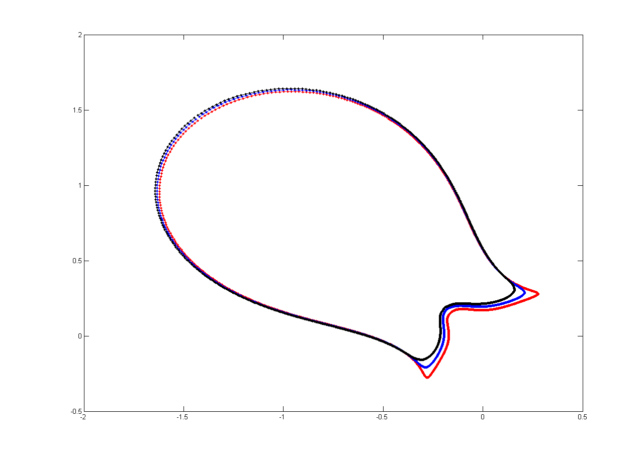
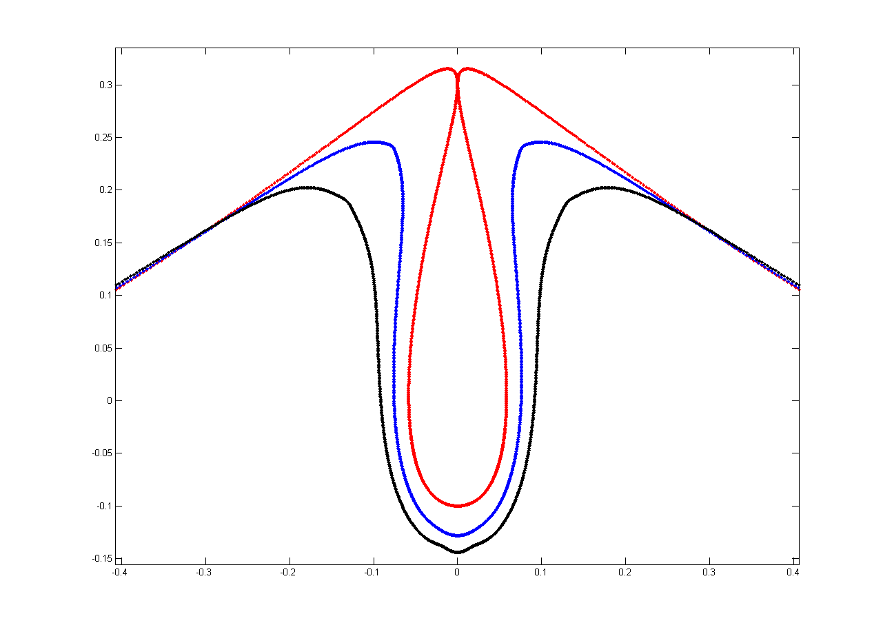
Figure 3: Tilde domain at times $t=0$ (Red - splash. The splash points are located on the open segment joining the points $(\sqrt{2}/2,\sqrt{2}/2)$ and $(-\sqrt{2}/2,-\sqrt{2}/2)$, approximately at $(\pm 0.27284156,\pm 0.27284156)$), $t=4\cdot 10^{-3}$ (Blue - turning) and $t=7\cdot 10^{-3}$ (Black - graph)

Figure 4: Zoom of the splash singularity at times $t=0$ (Red - splash), $t=4\cdot 10^{-3}$ (Blue - turning) and $t=7\cdot 10^{-3}$ (Black - graph)

6 Further research

We would like to exhibit a water-wave solution whose interface starts as an $H^{4}$-smooth graph at time zero, and ends in a splash at time $T$. We sketch a few ideas that may lead to a rigorous computer-assisted proof of the existence of such a solution. We will work in the tilde domain.

A simulation as in Section 5 leads to an approximate solution $x(\alpha,t)$, $\gamma(\alpha,t)$ with the desired properties. Thus $x(\cdot,t)$ describes a graph when $t=0$ and a splash when $t=T$. Moreover, we believe that equations similar to (14) hold, with very small $f$ and $g$.

We may suppose that $x$ and $\gamma$ are known piecewise-polynomial functions on $[0,2\pi]\times[0,T]$. Using interval arithmetic [16], one can compute rigorous upper bounds for appropriate Sobolev norms of $f$ and $g$. We hope that these upper bounds will be very small.

Next, we solve the water-wave equations (2-3) for $z,\omega$, starting at time $T$, and proceeding backwards in time. We take our initial $(z,\omega)$ at time $T$ to be a splash, very close to $(x(\cdot,T),\gamma(\cdot,T))$ in a high Sobolev norm.

We want to compare the exact solution $(z,\omega)$ with the approximate solution $(x,\gamma)$, using the quantity $\mathcal{E}(t)$ as in Theorem 4.1. Since $(z,\omega)$ and $(x,\gamma)$ are very close at time $T$, we will be able to show easily that

$$\mathcal{E}(T)<\varepsilon_{1},\text{ for a very small, computable constant $\varepsilon_{1}$.}$$ (15)

Moreover, the functions $x$ and $\gamma$ are known; and we also know upper bounds for Sobolev norms of $f$ and $g$. Therefore, the ideas in the proof of Theorem 4.1, together with interval arithmetic, should lead to a rigorous proof of the differential inequality

$$\left|\frac{d}{dt}\mathcal{E}(t)\right|\leq C_{1}\mathcal{E}(t)+\varepsilon_{2},$$ (16)

where $C_{1}$ and $\varepsilon_{2}$ are computable constants.

We hope that $\varepsilon_{2}$ is very small, since $f$ and $g$ have small Sobolev norms; and we hope that $C_{1}$ won’t be too big.

Once we establish (15) and (16), we will then know that our water wave solution $(z,\omega)$ exists for all time $t\in[0,T]$, and that $\mathcal{E}(0)<\varepsilon_{3}$ for a (hopefully small) computable constant $\varepsilon_{3}$.

From the definition of $\mathcal{E}(t)$, we will then easily deduce that $z(\cdot,0)-x(\cdot,0)$ has norm at most $\varepsilon_{4}$ in $H^{4}(\mathbb{R}/2\pi\mathbb{Z})$, for a computable constant $\varepsilon_{4}$.

If $\varepsilon_{4}$ is small enough, this in turn implies that the interface $z(\cdot,0)$ is an $H^{4}$-smooth graph. Thus $(z,\omega)$ is an exact solution of the water-wave equation, whose interface is an $H^{4}$-smooth graph at time 0, and a splash at time $T$.

We hope that a proof along these lines can be made to work.

Acknowledgements

AC, DC, FG and JGS were partially supported by the grant MTM2008-03754 of the MCINN (Spain) and the grant StG-203138CDSIF of the ERC. CF was partially supported by NSF grant DMS-0901040. FG was partially supported by NSF grant DMS-0901810.

Angel Castro
Instituto de Ciencias Matemáticas
Consejo Superior de Investigaciones Científicas
C/ Nicolás Cabrera, 13-15
Campus Cantoblanco UAM, 28049 Madrid
Email: angel castro@icmat.es
Diego Córdoba	Charles Fefferman
Instituto de Ciencias Matemáticas	Department of Mathematics
Consejo Superior de Investigaciones Científicas	Princeton University
C/ Nicolás Cabrera, 13-15	1102 Fine Hall, Washington Rd,
Campus Cantoblanco UAM, 28049 Madrid	Princeton, NJ 08544, USA
Email: dcg@icmat.es	Email: cf@math.princeton.edu
Francisco Gancedo	Javier Gómez-Serrano
Department of Mathematics	Instituto de Ciencias Matemáticas
University of Chicago	Consejo Superior de Investigaciones Científicas
5734 University Avenue,	C/ Nicolás Cabrera, 13-15
Chicago, IL 60637, USA	Campus Cantoblanco UAM, 28049 Madrid
Email: fgancedo@math.uchicago.edu	Email: javier.gomez@icmat.es

References

• [1] T. Alazard and G. Métivier. Paralinearization of the Dirichlet to Neumann operator, and regularity of three-dimensional water waves. Comm. Partial Differential Equations, 34(10-12):1632–1704, 2009.
• [2] B. Alvarez-Samaniego and D. Lannes. Large time existence for 3D water-waves and asymptotics. Invent. Math., 171(3):485–541, 2008.
• [3] D. M. Ambrose and N. Masmoudi. The zero surface tension limit of three-dimensional water waves. Indiana Univ. Math. J., 58(2):479–521, 2009.
• [4] J. T. Beale, T. Y. Hou, and J. Lowengrub. Convergence of a boundary integral method for water waves. SIAM J. Numer. Anal., 33(5):1797–1843, 1996.
• [5] J. T. Beale, T. Y. Hou, and J. S. Lowengrub. Growth rates for the linearized motion of fluid interfaces away from equilibrium. Comm. Pure Appl. Math., 46(9):1269–1301, 1993.
• [6] A. Castro, D. Córdoba, C. Fefferman, F. Gancedo, and M. López-Fernández. Rayleigh-Taylor breakdown for the Muskat problem with applications to water waves. Ann. of Math. (2), 2011. To appear.
• [7] A. Castro, D. Córdoba, C. Fefferman, F. Gancedo, and M. López-Fernández. Turning waves and breakdown for incompressible flows. Proceedings of the National Academy of Sciences, 108(12):4754–4759, 2011.
• [8] D. Christodoulou and H. Lindblad. On the motion of the free surface of a liquid. Comm. Pure Appl. Math., 53(12):1536–1602, 2000.
• [9] A. Córdoba, D. Córdoba, and F. Gancedo. Interface evolution: water waves in 2-D. Adv. Math., 223(1):120–173, 2010.
• [10] D. Coutand and S. Shkoller. Well-posedness of the free-surface incompressible Euler equations with or without surface tension. J. Amer. Math. Soc., 20(3):829–930, 2007.
• [11] W. Craig. An existence theory for water waves and the Boussinesq and Korteweg-de Vries scaling limits. Comm. Partial Differential Equations, 10(8):787–1003, 1985.
• [12] P. Germain, N. Masmoudi, and J. Shatah. Global solutions for the gravity water waves equation in dimension 3. C. R. Math. Acad. Sci. Paris, 347(15-16):897–902, 2009.
• [13] D. Lannes. Well-posedness of the water-waves equations. J. Amer. Math. Soc., 18(3):605–654, 2005.
• [14] D. Lannes. A stability criterion for two-fluid interfaces and applications. Arxiv preprint arXiv:1005.4565, 2010.
• [15] H. Lindblad. Well-posedness for the motion of an incompressible liquid with free surface boundary. Ann. of Math. (2), 162(1):109–194, 2005.
• [16] R. Moore and F. Bierbaum. Methods and applications of interval analysis, volume 2. Society for Industrial & Applied Mathematics, 1979.
• [17] V. I. Nalimov. The Cauchy-Poisson problem. Dinamika Splošn. Sredy, (Vyp. 18 Dinamika Zidkost. so Svobod. Granicami):104–210, 1974.
• [18] L. Nirenberg. An abstract form of the nonlinear Cauchy-Kowalewski theorem. J. Differential Geometry, 6:561–576, 1972. Collection of articles dedicated to S. S. Chern and D. C. Spencer on their sixtieth birthdays.
• [19] T. Nishida. A note on a theorem of Nirenberg. J. Differential Geom., 12(4):629–633, 1977.
• [20] L. Rayleigh. On the instability of jets. Proceedings of the London Mathematical Society, s1-10(1):4–13, 1878.
• [21] J. Shatah and C. Zeng. Geometry and a priori estimates for free boundary problems of the Euler equation. Comm. Pure Appl. Math., 61(5):698–744, 2008.
• [22] G. Taylor. The instability of liquid surfaces when accelerated in a direction perpendicular to their planes. I. Proc. Roy. Soc. London. Ser. A., 201:192–196, 1950.
• [23] S. Wu. Well-posedness in Sobolev spaces of the full water wave problem in $2$-D. Invent. Math., 130(1):39–72, 1997.
• [24] S. Wu. Well-posedness in Sobolev spaces of the full water wave problem in 3-D. J. Amer. Math. Soc., 12(2):445–495, 1999.
• [25] S. Wu. Almost global wellposedness of the 2-D full water wave problem. Invent. Math., 177(1):45–135, 2009.
• [26] S. Wu. Global wellposedness of the 3-D full water wave problem. Invent. Math., 184(1):125–220, 2011.
• [27] H. Yosihara. Gravity waves on the free surface of an incompressible perfect fluid of finite depth. Publ. Res. Inst. Math. Sci., 18(1):49–96, 1982.
• [28] P. Zhang and Z. Zhang. On the free boundary problem of three-dimensional incompressible Euler equations. Comm. Pure Appl. Math., 61(7):877–940, 2008.