On Quantum Channel Estimation
with Minimal Resources

Abstract

We determine the minimal experimental resources that ensure a unique solution in the estimation of trace-preserving quantum channels with both direct and convex optimization methods. A convenient parametrization of the constrained set is used to develop a globally converging Newton-type algorithm that ensures a physically admissible solution to the problem. Numerical simulations are provided to support the results, and indicate that the minimal experimental setting is sufficient to guarantee good estimates.

1 Introduction

Recent advances and miniaturization in laser technology and electronic devices, together with some profound results in quantum physics and quantum information theory, have generated in the last two decades increasing interest in the promising field of quantum information engineering. The potential of these new technologies have been demonstrated by a number of theoretical and experimental results, including intrinsically-secure quantum cryptography protocols, proof-of-principle implementation of quantum computing, as well as dramatic advances in controlled engineering of molecular dynamics, opto-mechanical devices, and many other experimentally available systems. In this area, a key role is played by control, estimation and identification problems for quantum-mechanical systems [15, 38, 32, 31, 21]. Important contributions to this multi-disciplinary research effort have been offered by a number control scientists, among which we would like to remember Mohammed Daleh. A few examples dealing with control and estimation problems are [13, 14, 16, 5, 4, 18, 36, 30, 24, 23, 34, 6, 27], and many more may be found in the surveys [1, 19].
In the spirit of developing research which is both strongly motivated by emerging applications and mathematically rigorous, we consider an identification problem arising in the reconstruction of quantum dynamical models from experimental data. This is a key issue in many quantum information processing tasks [29, 11, 31, 28, 10]. For example, a precise knowledge of the behavior of a channel to be used for quantum computation or communications is needed in order to ensure that optimal encoding/decoding strategies are employed, and verify that the noise thresholds for hierarchical error-correction protocols, or for effectiveness of quantum key distribution protocols, are met [29, 11]. In many cases of interest, for example in communication in free-space [37], channels are not stationary and to ensure good performances, repeated and fast estimation steps would be needed as a prerequisite for adaptive information encodings. Motivated by these potential applications, we here focus on: (i) characterizing the minimum experimental setting needed for a consistent estimation of the channel; (ii) exploring how a minimal parametrization of the models can be exploited to reduce the complexity of the estimation algorithm; and (iii) testing (numerically) the minimal experimental setting, and compare it to “richer” experimental resources (in terms of available probe states and measured observables). In doing this, we present a general framework for the estimation of physically-admissible trace preserving quantum channels by minimizing a suitable class of (convex) loss functions which contains, as special cases, commonly used maximum likelihood (ML) functionals. In the large body of literature regarding channel estimation, or quantum process tomography (see e.g. [31, 28] and references therein), the experimental resources are usually assumed to be given. Mohseni et al. [28] compare different strategies, but focus on the role of having entangled states as an additional resource, while we shall assume there is no additional quantum system to work with. The problem we study is closer in spirit to that taken in [35] while studying minimal state tomography.
Our result include the determination of the minimal experimental resources (or quorum, in the language of [17]) for Trace-Preserving (TP) channels estimation, as part of a thorough theoretical analysis of both the inversion (direct, or standard tomography) method and a class of convex methods, including the widely-used maximum likelihood approach. The method we propose constrains the set of channels of the optimization problem to TP maps from the beginning, as opposed to the most common approach that introduces the TP constraint through a Lagrange multiplier [31, 28]. This allow for an immediate reduction from $d^{4}$ to $d^{4}-d^{2}$ parameters in estimation problem. Our analysis can also be considered as complementary to the one presented in [9], where the TP assumption is relaxed to include losses. We provide a rigorous presentation of the results and we try, whenever possible, to make contact with ideas and methods of (classical) system identification. We next exploit the same convenient parametrization for TP channels we use in the theoretical analysis for developing a Newton-type algorithm with barriers, which ensures convergence in the set of physically-admissible maps. Numerical simulations are provided, confirming that the standard tomography method quite often fails to provide a positive map, and showing that experimental settings richer than the minimal one (in terms of input states and observables) do not lead to better performances (fixed the total number of available ”trials”).

2 Quantum channels and $\chi$-representation

Consider a $d$-level quantum system with associated Hilbert space $\mathcal{H}$ isomorphic to ${\mathbb{C}}^{d}$. The state of the system is described by a density operator, namely by a positive, unit-trace matrix

$$\rho\in\mathfrak{D}(\mathcal{H})=\{\rho\in\mathbb{C}^{d\times d}|\rho=\rho^{\dagger}\geq 0,\,\textrm{tr}(\rho)=1\},$$

which plays the role of probability distribution in classical probability. A state is called pure if it has rank one, and hence it is represented by an orthogonal projection matrix on a one-dimensional subspace. Measurable quantities or observables are associated with Hermitian matrices $X=\sum_{k}x_{k}\Pi_{k},$ with $\{\Pi_{k}\}$ the associated spectral family of orthogonal projections. Their spectrum $\{x_{k}\}$ represents the possible outcomes, and the probability of observing the $k$th outcome can be computed as $p_{\rho}(\Pi_{k})=\textrm{tr}(\Pi_{k}\rho).$

A quantum channel (in Schrödinger’s picture) is a map $\mathcal{E}:\mathfrak{D}(\mathcal{H})\rightarrow\mathfrak{D}(\mathcal{H}).$ It is well known [26, 29] that a physically admissible quantum channel must be linear and Completely Positive (CP), namely it admits an Operator-Sum Representation (OSR)

$$\mathcal{E}(\rho)=\sum_{j=1}^{d^{2}}K_{j}\rho K_{j}^{\dagger}$$ (1)

where $K_{i}\in\mathbb{C}^{d\times d}$ are called Kraus operators. In order to be Trace Preserving (TP), a necessary condition to map states to states, it must also hold that

$$\sum_{j=1}^{d^{2}}K_{j}^{\dagger}K_{j}=I_{d}$$ (2)

where $I_{d}$ is the $d\times d$ identity matrix.

An alternative way to describe a CPTP channel is offered by the $\chi$-representation. Each Kraus operator $K_{j}\in\mathbb{C}^{d\times d}$ can be expressed as a linear combination (with complex coefficients) of $\{F_{m}\}_{m=1}^{d^{2}}$, $F_{m}$ being the elementary matrix $E_{jk},$ with $m=(j-1)d+k.$ Accordingly, the OSR (1) can be rewritten as

$$\mathcal{E}(\rho)=\sum_{m,n=1}^{d^{2}}\chi_{m,n}F_{m}\rho F_{n}^{\dagger}$$ (3)

where $\chi$ is the $d^{2}\times d^{2}$ Hermitian matrix with element $\chi_{m,n}$ in position $(m,n)$. It easy to see that it must satisfy

$$\chi=\chi^{\dagger}\geq 0$$ (4)

and (following from (2))

$$\sum_{m,n=1}^{d^{2}}\chi_{m,n}F_{n}^{\dagger}F_{m}=I_{2}.$$ (5)

The map $\mathcal{E}$ is completely determined by the matrix $\chi$.

We now introduce an helpful lemma which provides us with a parametrization of trace preserving maps, and an easy formula for computing probabilities in terms $\chi$ . For a brief review of the partial trace definition and properties, see the Appendix A.

Lemma 2.1

Let $\mathcal{E}_{\chi}$ be a CPTP map associated with a given $\chi$. Then for any $\rho\in\mathfrak{D}(\mathcal{H})$

$$\mathcal{E}_{\chi}(\rho)=\textrm{tr}_{2}(\chi(I_{d}\otimes\rho^{T})).$$ (6)

Proof. Let us rewrite each $F_{j}$ as the corresponding elementary matrix $E_{lm},$ with $j=(l-1)d+m,\,k=(n-1)d+p,$ and relabel $\chi_{jk}$ as $\hat{\chi}_{lmnp}$ accordingly. Hence we get

$$\chi=\sum_{l,m,n,p}\hat{\chi}_{lmnp}E_{ln}\otimes E_{mp},$$ (7)

and

$$\mathcal{E}_{\chi}(\rho)=\sum_{l,m,n,p}\hat{\chi}_{lmnp}E_{lm}\rho E_{pn}.$$

We can also expand $\rho=\sum_{rs}\rho_{rs}E_{rs},$ and substitute it in the above expression. Taking into account that $E_{lm}E_{np}=\delta_{mn}E_{lp}$, and defining $[\hat{\chi}^{B}_{ln}]_{mp}=\hat{\chi}_{lmnp}$, we get:

$$\mathcal{E}_{\chi}(\rho) = \sum_{l,m,n,p,r,s}\rho_{rs}\hat{\chi}_{lmnp}E_{lm}E_{rs}E_{pn}$$

$$= \sum_{l,n,r,s}\rho_{rs}\hat{\chi}_{lrns}E_{ln},$$

$$= \sum_{l,n}\left(\sum_{r,s}\rho_{rs}\hat{\chi}_{lrns}\right)E_{ln}$$

$$= \sum_{l,n}\left(\rho^{T}\hat{\chi}^{B}_{ln}\right)E_{ln},$$

$$= \textrm{tr}_{2}(\chi(I\otimes\rho^{T}))$$

where we used the fact that $\hat{\chi}^{B}_{ln}$ corresponds to the $d\times d$ dimensional block of $\chi$ in position $(l,n),$ and that for every pair of matrices $X,Y,$ we can write $\sum_{rs}X_{rs}Y_{rs}=\textrm{tr}(X^{T}Y).$ $\Box$

This leads to a useful expression for the computation of the expectations.

Corollary 2.1

Let us consider a state $\rho$, a projector $\Pi$ and a quantum channel $\mathcal{E}$ with associated $\chi$-representation matrix $\chi$. Then

$${\color[rgb]{0,0,0}p_{\mathcal{E}(\rho)}(\Pi)}=\textrm{tr}(\mathcal{E}(\rho)\Pi)=\textrm{tr}(\chi(\Pi\otimes\rho^{T})).$$

Proof. It suffices to substitute (6) in $p_{\chi,\rho}(\Pi)=\textrm{tr}(\mathcal{E}(\rho)\Pi),$ and use the identity $\textrm{tr}(X\otimes I)Y)=\textrm{tr}(X\textrm{tr}_{2}(Y)).$ $\Box$

The TP condition (5) can also be re-expressed directly in terms of the $\chi$ matrix.

Corollary 2.2

Let us consider a CP map $\mathcal{E}_{\chi}$ with associated $\chi$-representation matrix $\chi$. Then $\mathcal{E}_{\chi}$ is TP if and only if

$$\textrm{tr}_{1}(\chi)=I_{d}.$$ (8)

Proof. Using the same notation we used in the proof of Lemma 2.1, we can re-espress the TP condition (5) as:

$$I_{d}=\sum_{l,m,n,p}\hat{\chi}_{lmnp}E_{pn}E_{lm}=\sum_{l,m,p}\hat{\chi}_{lmlp}E_{pm}=\textrm{tr}_{1}(\chi).$$

$\Box$

3 Identification Protocols

Consider the following setting: a quantum system prepared in a known pure state $\rho$ is fed to an unknown channel ${\mathcal{E}}.$ The system in the output state $\mathcal{E}(\rho)$ is then subjected to a projective measurement of an observable: to our aim it will be sufficient to consider yes-no measurements associated to orthogonal projections $\Pi=\Pi^{\dagger}=\Pi^{2}.$ Hence the outcome $x$ is in the set $\{0,1\},$ and can be interpreted as a sample of the random variable $X$ which has distribution

$$P_{\chi(x),{\color[rgb]{0,0,0}\rho}}=\left\{\begin{array}[]{ll}p_{\chi,\rho}(\Pi),&\;\;\hbox{if }x=1\\ 1-p_{\chi,\rho}(\Pi),&\;\;\hbox{if }x=0\end{array}\right.$$ (9)

where $p_{\chi,\rho}(\Pi)=\textrm{tr}(\mathcal{E}_{\chi}(\rho)\Pi)$ is the probability that the measurement of $\Pi$ returns outcome 1 when the state is $\mathcal{E}_{\chi}(\rho)$.

Assume that the experiment is repeated with a series of known input (pure) states $\{\rho_{k}\}_{{\color[rgb]{0,0,0}k=1}}^{{\color[rgb]{0,0,0}L}}$, and to each trial the same orthogonal projections $\{\Pi_{j}\}_{{\color[rgb]{0,0,0}j=1}}^{{\color[rgb]{0,0,0}M}}$ are measured $N$ times, obtaining a series of outcomes $\{x_{l}^{jk}\}$. We consider the sampled frequencies to be our data, namely

$$f_{jk}:=\frac{1}{N}\sum_{l=1}^{N}x_{l}^{jk}.$$ (10)

The channel identification problem (or as it is referred to in the physics literature, the quantum process tomography problem [31, 29, 28]) we are concerned with consists in constructing a Kraus map ${\mathcal{E}}_{\hat{\chi}}$ that fits the experimental data (in some optimal way), in particular estimating a matrix $\hat{\chi}$ satisfying constraints (3),(4).

3.1 Necessary and sufficient conditions for identifiability

It is well known [33, 31] that by imposing linear constraints associated to the TP condition (5), or equivalently (8), one reduces the $d^{4}$ real degrees of freedom of $\chi$ to $d^{4}-d^{2}.$ This will be made explicit in the following, by parameterizing $\chi$ in a “generalized” Pauli basis (also known as gell-mann matrices, Fano basis or coherence vector representation in the case of states [3, 7, 31]). Usually the trace preserving constraint is not directly included in the standard tomography method [28], since in principle it should emerge from the physical properties of the channel, or it is imposed through a (nonlinear) Lagrange multiplier in the maximum likelihood approach [31]. Here, in order to investigate the minimum number of probe (input) states and measured projectors needed to uniquely determine $\chi$, it is convenient to include this constraint from the very beginning. Doing so, we lose the possibility of exploiting a Cholesky factorization in order to impose positive semidefiniteness of $\chi$: noentheless, we show in Section 3.5 that semidefiniteness of the solution can be imposed algorithmically by using a barrier method [12].

Consider an orthonormal basis for $d^{2}\times d^{2}$ Hermitian matrices of the form $\{\sigma_{j}\otimes\sigma_{k}\}_{j,k=0,1,\dots,d^{2}-1},$ where $\sigma_{0}=1/\sqrt{d}I_{d},$ while $\{\sigma_{j}\}_{j=1,\dots,d^{2}-1}$ is a basis for the traceless subspaces. We can now write

$$\chi=\sum_{jk}s_{jk}\sigma_{j}\otimes\sigma_{k}.$$

If we now substitute it into (8), we get:

$$I_{d}=\textrm{tr}_{1}(\chi)=\sum_{jk}s_{jk}\textrm{tr}(\sigma_{j})\sigma_{k}\\ =\sum_{k}\sqrt{d}\,s_{0k}\sigma_{k},$$

and hence, since the $\sigma_{j}$ are linearly independent, we can conclude that $s_{00}=1,\,s_{0j}=0$ for $j=1,\ldots,d^{2}-1.$ Hence, the free parameters for a TP map (at this point not necessarily CP, since we have not imposed the positivity of $\chi$ yet) are $d^{4}-d^{2},$ as we can write any TP $\chi$ as $\chi=d^{-1}I_{d^{2}}+\sum_{j=1,k=0}^{d^{2}{\color[rgb]{0,0,0}-1},d^{2}{\color[rgb]{0,0,0}-1}}s_{jk}\sigma_{j}\otimes\sigma_{k},$ or, in a more compact notation,

$$\chi(\underline{\theta})=d^{-1}I_{d^{2}}+\sum_{\ell=1}^{d^{4}-d^{2}}\theta_{\ell}Q_{\ell},$$ (11)

by rearranging the double index $j,k$ in a single $\ell,$ and defining the corresponding $Q_{\ell}=\sigma_{j}\otimes\sigma_{k}.$

The $\chi$ matrices corresponding to TP maps thus form an affine space. Let us call it linear part

$${\mathcal{S}}_{TP}=\textrm{span}\{\sigma_{j}\otimes\sigma_{k}\}_{j=1,\ldots,d^{2}{\color[rgb]{0,0,0}-1},k=0,\ldots,d^{2}{\color[rgb]{0,0,0}-1}}.$$

It is convenient to define

$$B_{jk}=(\Pi_{j}-\frac{1}{d}I)\otimes\rho^{T}_{k}$$ (12)

and ${\mathcal{B}}=\textrm{span}\{B_{jk}\}_{j=1,\ldots,{\color[rgb]{0,0,0}M},k=1,\dots,{\color[rgb]{0,0,0}L}}.$ Since we have $Q_{\ell}=\sigma_{j\neq 0}\otimes\sigma_{k},$ it holds that

$$\textrm{tr}(Q_{\ell}(\Pi_{j}\otimes\rho^{T}_{k}))=\textrm{tr}(Q_{\ell}B_{jk}).$$ (13)

Let us also introduce the function

$$\hskip 56.9055ptg : \mathbb{R}^{d^{4}-d^{2}}\rightarrow\mathbb{R}^{{\color[rgb]{0,0,0}M\times L}}$$

$$\underline{\theta}\mapsto g(\underline{\theta})$$

with the component of $g(\underline{\theta})$ in position $(j,k)$ is defined as

$$g_{jk}(\underline{\theta})=p_{\chi(\underline{\theta}),\rho_{k}}(\Pi_{j})=\textrm{tr}(\chi(\underline{\theta})(\Pi_{j}\otimes\rho^{T}_{k})).$$ (14)

Proposition 3.1

$g$ is injective if and only if $\mathcal{S}_{TP}\subset\mathcal{B}$.

Proof. Given (14), we have that

$$g_{jk}(\underline{\theta}_{1})-g_{jk}(\underline{\theta}_{2}) = \textrm{tr}[(\chi(\underline{\theta}_{1})-\chi(\underline{\theta}_{2}))(\Pi_{j}\otimes\rho^{T}_{k})]$$

$$= \textrm{tr}[S(\underline{\theta}_{1}-\underline{\theta}_{2})B_{jk}]$$

$$= \langle S(\underline{\theta}_{1}-\underline{\theta}_{2}),B_{jk}\rangle$$

where $S(\underline{\theta}_{1}-\underline{\theta}_{2})=\chi(\underline{\theta}_{1})-\chi(\underline{\theta}_{2})=\sum_{l=1}^{d^{4}-d^{2}}(\theta_{1,l}-\theta_{2,l})Q_{l}\in\mathcal{S}_{TP}.$ So, we have that

$$g(\underline{\theta}_{1})=g(\underline{\theta}_{2})\;\Leftrightarrow\;\langle S(\underline{\theta}_{1}-\underline{\theta}_{2}),B_{jk}\rangle=0\;\;\forall\;j,k.$$ (15)

Assume $\mathcal{S}_{TP}\subset\mathcal{B}:$ the only element of ${\mathcal{S}}_{TP}$ for which the r.h.s. of (15) could be true is zero. Since by definition $S(\underline{\theta}_{1}-\underline{\theta}_{2})=0$ if and only if $\underline{\theta}_{1}=\underline{\theta}_{2}$ , $g$ is injective. On the other hand, assume that $\mathcal{S}_{TP}\not\subseteq\mathcal{B}:$ therefore there exists $T\neq 0\in\mathcal{S}_{TP}\bigcap{\mathcal{B}}^{\perp}$ such that

$$T=\sum_{\ell}\gamma_{\ell}Q_{\ell},\quad\langle T,B_{jk}\rangle=0\;\forall j,k.$$

But this would mean that $\underline{\theta}$ and $\underline{\theta}+\underline{\gamma}$ have the same image $g(\underline{\theta})$, and hence $g$ is not injective. $\Box$

This is a central result in our analysis: we anticipate here that $g$ being injective is a necessary and sufficient condition for a priori identifiability of $\chi,$ and thus for having a unique solution of the problem for both inversion (standard process tomography) and convex optimization-based (e.g. maximum likelihood) methods, up to some basic assumptions on the cost functional. The proof is given in full detail in Section 3.2 and 3.3.

As a consequence of these facts, we can determine the minimal experimental resources, in terms of input states and measured projectors, needed for faithfully reconstructing $\chi$ from noiseless data $\{f^{\circ}_{jk}\}$, where $f^{\circ}_{jk}=p_{\chi,\rho}(\Pi)$. In the light of proposition 3.1, the minimal experimental setting is characterized by a choice of $\{\Pi_{j},\rho_{k}\}$ such that ${\mathcal{S}}_{TP}={\mathcal{B}}$. Recalling the definition of ${\mathcal{B}},$ through (12), it is immediate to see that ${\mathcal{S}}_{TP}={\mathcal{B}}$ if and only if $\textrm{span}\{\Pi_{j}-d^{-1}I_{d}\}=\textrm{span}\{\sigma_{j},j=1,\ldots,d^{2}{\color[rgb]{0,0,0}-1}\}$ and $\textrm{span}\{\rho_{k}\}=\mathbb{C}^{d\times d}.$ We can summarize this fact as a corollary of Proposition 3.1.

Corollary 3.1

$g$ is injective if and only if we have at least $d^{2}$ linearly independent input states $\{\rho_{k}\},$ and $d^{2}-1$ measured $\{\Pi_{j}\}$ such that

$$\textrm{span}\{\Pi_{j}-d^{-1}I_{d}\}=\textrm{span}\{\sigma_{j},j=1,\ldots,d^{2}{\color[rgb]{0,0,0}-1}\}.$$

We call such a set a minimal experimental setting. Notice that, using the terminology of [31, 17], the minimal quorum of observables consists of $d^{2}-1$ properly chosen elements. While in most of the literature at least $d^{2}$ observables are considered [20, 28], we showed it is in principle possible to spare a measurement channel at the output. A physically-inspired interpretation for this fact is that, since we a priori know, or assume, that the channel is TP, measuring the component of the observables along the identity does not provide useful information. This is clearly not true if one relaxes the TP condition, as it has been done in [9]: in that case, by the same line of reasoning, $d^{2}$ linearly independent observables are the necessary and sufficient for $g$ to be injective.

As an example relevant to many experimental situation, consider the qubit case, i.e. $d=2.$ A minimal set of projector has to span the traceless subspace of $\mathbb{C}^{2\times 2}$: one can choose e.g.:

$$\Pi_{j}=\frac{1}{2}I_{2}+\sigma_{j},\;j=x,y,z.$$

$$\rho_{x,y}=\frac{1}{2}I_{2}+\sigma_{x,y},\quad\rho_{\pm}=\frac{1}{2}I_{2}\pm\sigma_{z}.$$ (16)

It is clear that there is an asymmetry between the role of output and inputs: in fact, exchanging the number of $\{\Pi_{j}\}$ and $\{\rho_{k}\}$ can not lead to an injective $g$.

3.2 Process Tomography by inversion

Assume that $\mathcal{S}_{TP}\subset\mathcal{B},$ and that the data $\{f_{jk}\}$ have been collected. Since $f_{jk}$ is an estimate of $p_{\chi(\underline{\theta}),\rho_{k}}(\Pi_{j})$, consider the following least mean square problem

$$\min_{\underline{\theta}\in\mathbb{R}^{d^{4}-d^{2}}}\|\underline{g}(\underline{\theta})-\underline{f}\|$$ (17)

where $\underline{g}(\underline{\theta})$ and $\underline{f}$ are the vectors obtained by stacking the $g_{jk}(\underline{\theta})$ and $f_{jk}$ $j=1\ldots L,$ $k=\ldots M$, respectively. In view of (11) and (14) we have that $\underline{g}(\underline{\theta})=T\underline{\theta}+d^{-1}\underline{1}$ where

$$T=\left[\begin{array}[]{ccc}\ddots&\vdots&\\ &\textrm{tr}(B_{jk}Q_{\ell})&\\ &\vdots&\ddots\end{array}\right]$$ (18)

and $\underline{1}$ is a vector of ones. Notice that the $\ell$th column of $T$ is formed with the inner products of $Q_{\ell}$ with each $B_{jk}.$ Since $\mathcal{S}_{TP}\subset\mathcal{B}$, the $Q_{\ell}$ are linearly independent and the $B_{jk}$ are the generators of ${\mathcal{B}},$ then $T$ is full column rank, namely has rank $d^{4}-d^{2}$. Hence, in principle, one can reconstruct $\hat{\theta}$ as

$${\color[rgb]{0,0,0}\hat{}\underline{\theta}}=T^{\#}(\underline{f}-\underline{1}),$$ (19)

$T^{\#}$ being the Moore-Penrose pseudo inverse of $T$ [22]. If the experimental setting is minimal, the usual inverse suffices. However, as it is well known, when computing $\chi$ this way from real (noisy) data, the positivity character is typically lost [31, 2]. We better illustrate this fact in Section 4, through numerical simulations.

3.3 Convex methods: general framework

More robust approaches for the estimation of physically-acceptable $\chi$ (or equivalent parametrizations) have been developed, most notably by resorting to Maximum Likelihood methods [20, 33, 31, 39]. The optimal channel estimation problem can be stated, by using the parametrization for $\chi(\underline{\theta})=d^{-1}I_{d^{2}}+\sum_{\ell}\theta_{\ell}Q_{\ell}$ presented in the previous section, as it follows: consider a set of data $\{f_{jk}\}$ as above, and a cost functional $J(\underline{\theta}):=h\circ g(\underline{\theta})$ where $h:\mathbb{R}^{M\times L}\rightarrow\mathbb{R}$ is a suitable function which depends on the data $\{f_{jk}\}$. We aim to find

$${\color[rgb]{0,0,0}\hat{\theta}=\arg\min_{\underline{\theta}}J(\underline{\theta})}$$ (20)

subject to $\underline{\theta}$ belonging to some constrained set ${\mathcal{C}}\subset\mathbb{R}^{d^{4}-d^{2}}$. In our case

$${\mathcal{C}}={\mathcal{A}}_{+}\quad{\rm or}\quad{\mathcal{C}}={\mathcal{A}}_{+}\cap{\mathcal{I}},$$

with ${\mathcal{A}}_{+}=\{{\color[rgb]{0,0,0}\underline{\theta}}\;|\;\chi(\theta)\geq 0\},$ while ${\mathcal{I}}=\{\underline{\theta}\;|\;0<\textrm{tr}(\chi(\underline{\theta})(\Pi_{j}\otimes\rho^{T}_{k}))<1,\;\forall\,j,k\}.$ The second constraint may be used when a cost functional which is not well-defined for extremal probabilities, or in order to ensure that the estimated channel exhibits some noise in each of the measured directions, as it is expected in realistic experimental settings. Since the analysis does not change significantly in the two settings, we will not distinguish between them where it is not strictly necessary. The following result will be instrumental to prove the existence of a unique solution.

Proposition 3.2

${\mathcal{C}}$ is a bounded set.

Proof. Since $\mathcal{C}\subset{\mathcal{A}}_{+}$, it is sufficient to show that ${\mathcal{A}_{+}}$ is bounded or, equivalently, that a sequence $\{\underline{\theta}_{j}\}_{j\geq 0}$, with $\underline{\theta}_{j}\in\mathbb{R}^{d^{4}-d^{2}}$, and $\|\underline{\theta}_{j}\|\rightarrow+\infty$, cannot belong to ${\mathcal{A}_{+}}$. To this end, it is sufficient to show that, as $\|\underline{\theta}_{j}\|\rightarrow+\infty$, the minimum eigenvalue of $\chi(\underline{\theta}_{j})$ tends to $-\infty$ so that, for $j$ large enough, $\underline{\theta}_{j}$ does not satisfy condition $\chi(\underline{\theta}_{j})\geq 0$. Notice that the map $\underline{\theta}\mapsto\chi(\underline{\theta})$ is affine. Moreover, since the $Q_{\ell}$s are lineraly independent, this map is injective. Accordingly, $\|\chi(\underline{\theta}_{j})\|$ approach infinity as $\|\underline{\theta}_{j}\|\rightarrow+\infty$. Since $\chi(\underline{\theta}_{j})$ is a Hermitian matrix, $\chi(\underline{\theta}_{j})$ has an eigenvalue $\lambda_{j}$ such that $|\lambda_{j}|\rightarrow+\infty$ as $\|\chi(\underline{\theta}_{j})\|\rightarrow+\infty$. Recall that $\chi(\underline{\theta}_{j})$ satisfies (8) by construction which implies that $\textrm{tr}(\chi(\underline{\theta}_{j}))=d$ namely the sum of its eigenvalues is always equal to $d$. Thus, there exists an eigenvalue of $\chi(\underline{\theta}_{j})$ which approaches $-\infty$ as $j\rightarrow+\infty$, which is in contrast with its positivity. So, $\mathcal{C}$ is bounded. $\Box$

Here we focus on the following issue: under which conditions on the experimental setting (or, mathematically, on the set ${\mathcal{B}}$ defined above) do the optimization approach have a unique solution? In either of the cases above, ${\mathcal{C}}$ is the intersection of convex nonempty sets: in fact, ${\mathcal{S}}_{TP}$ and $\chi\geq 0$ are convex and so must be the corresponding sets of $\underline{\theta}$, and it is immediate to verify that ${\mathcal{I}}$ is convex as well; all of these contain $\underline{\theta}=0,$ corresponding to $\frac{1}{d}I_{d^{2}},$ and hence they are non empty. In the light of this, it is possible to derive sufficient conditions on $J$ for existence and uniqueness of the minimum in the presence of arbitrary constraint set ${\mathcal{C}}.$ Define $\partial{\mathcal{C}}_{0}:=\partial{\mathcal{C}}\setminus(\partial{\mathcal{C}}\cap{\mathcal{A}}_{+})$

Proposition 3.3

Assume $h$ is continuous and strictly convex on $g({\mathcal{C}})$, and

$$\lim_{\underline{\theta}\rightarrow\partial\mathcal{C}_{0}}J(\underline{\theta})=\lim_{\underline{\theta}\rightarrow\partial\mathcal{C}_{0}}h\circ g(\underline{\theta})=+\infty.$$ (21)

If $\mathcal{S}_{TP}\subset\mathcal{B}$, then the functional $J$ has a unique minimum point in $\mathcal{C}$.

Proof. Since $h$ is strictly convex on $g(\mathcal{C})$ and the linear function $g$, in view of Proposition 3.1, is injective on $\mathcal{C}$, $J$ is strictly convex on $\mathcal{C}$. So, we only need to show that $J$ takes a minimum value on $\mathcal{C}$. In order to do so, it is sufficient to show that $J$ is inf-compact, i.e., the image of $(-\infty,r]$ under the map $J^{-1}$ is a compact set. Existence of the minimum for $J$ then follows from a version of Weierstrass theorem since an inf-compact function has closed level sets, and is therefore, lower semicontinuous [25, p. 56]. Define $\underline{\theta}_{0}:=\left(\begin{array}[]{ccccc}0&\ldots&0\\ \end{array}\right)^{T}\in\mathbb{R}^{d^{4}-d^{2}}$. Observe that $\chi(\underline{\theta}_{0})={d}^{-1}I_{d^{2}}\geq 0$. Moreover, being $\Pi_{j}\otimes\rho^{T}_{k}$ rank-one orthogonal projections

$$\textrm{tr}(\chi(\underline{\theta}_{0})\Pi_{j}\otimes\rho^{T}_{k})=\frac{1}{d}\;\;\forall j,k.$$ (22)

Therefore, $\underline{\theta}_{0}\in{\color[rgb]{0,0,0}\mathcal{C}}$ and call $J(\underline{\theta}_{0})=J_{0}<\infty$. So, we can restrict the search for a minimum point to the image of $(-\infty,J_{0}]$ under $J^{-1}$. Since ${\mathcal{C}}$ is a bounded set by construction, to prove inf-compactness of $J$ it is sufficient to guarantee that

$$\lim_{\underline{\theta}\rightarrow\partial\mathcal{C}_{0}}J(\underline{\theta})=+\infty.$$

$\Box$

3.4 Maximum Likelihood functionals

3.4.1 Binomial functional

Assume a certain set of data $\{f_{jk}\}$ have been obtained, by repeating $N$ times the measurement of each pair $(\rho_{k},\Pi_{j})$. For technical reasons (strict convexity of the ML functional on the optimization set) and experimental considerations (noise typically irreversibly affects any state), it is typically assumed that $0<f_{jk}<1.$ The probability of obtaining a series of outcomes with $c_{jk}=f_{jk}N$ ones for the pair $(j,k)$ is then

$$P_{\chi}(c_{jk})={N\choose c_{jk}}\textrm{tr}(\chi\Pi_{j}\otimes\rho_{k}^{T})^{c_{jk}}[1-\textrm{tr}(\chi\Pi_{j}\otimes\rho_{k}^{T})]^{N-c_{jk}}$$ (23)

so that the overall probability of $\{c_{jk}\}$, may be expressed as: $P_{\chi}({\color[rgb]{0,0,0}\{c_{jk}\}})=\prod_{j=1}^{\color[rgb]{0,0,0}L}\prod_{k=1}^{\color[rgb]{0,0,0}M}P_{\chi}(c_{jk}).$ By adopting the Maximum Likelihood (ML) criterion, once fixed the $\{c_{jk}\}$ describing the recorded data, the optimal estimate $\hat{\chi}$ of $\chi$ is given by maximizing $P_{\chi}(\{c_{jk}\})$ with respect to $\chi$ over a suitable set $\mathcal{C}$. Let us consider our parametrization of the TP $\chi(\underline{\theta})$ as in (11) . If we assume $0<\textrm{tr}(\chi(\underline{\theta})(\Pi_{j}\otimes\rho_{k}^{T}))<1,$ since the logarithm function is monotone, it is equivalent (up to a constant emerging from the binomial coefficients) to minimize over $\mathcal{C}={\mathcal{A}}_{+}\cap{\mathcal{I}}$ the function

$$J(\underline{\theta}) = -\frac{1}{N}\log P_{\chi(\underline{\theta})}(\{c_{jk}\})+\sum_{j,k}\log\left(\begin{array}[]{c}N\\ c_{jk}\\ \end{array}\right)$$ (27)

$$= -\sum_{j,k}f_{jk}\log[\textrm{tr}(\chi(\underline{\theta})(\Pi_{j}\otimes\rho_{k}^{T})]$$

$$+(1-f_{jk})\log[1-\textrm{tr}(\chi(\underline{\theta})(\Pi_{j}\otimes\rho_{k}^{T}))].$$

Here, $h(X)=-\sum_{j,k}f_{jk}\log(x_{jk})+(1-f_{jk})\log(1-x_{jk})$ with $x_{jk}=[X]_{jk}$ and $X\in\mathbb{R}^{M\times L}$ is strictly convex on $\mathbb{R}^{M\times L}$ because $0<f_{jk}<1$ by assumption. Notice that $\partial\mathcal{C}_{0}$ is the set of $\underline{\theta}\in{\mathcal{A}}_{+}$ for which there exists at least one pair $(\tilde{i},\tilde{k})$ such that $\textrm{tr}(\chi(\underline{\theta})(\Pi_{\tilde{j}}\otimes\rho_{\tilde{k}}^{T}))=0,1.$ Suppose that $\textrm{tr}(\chi(\underline{\theta})(\Pi_{\tilde{j}}\otimes\rho_{\tilde{k}}^{T})\rightarrow 0$ as $\underline{\theta}\rightarrow\partial\mathcal{C}_{0}$. Therefore, $\log[\textrm{tr}(\chi(\underline{\theta})(\Pi_{j}\otimes\rho_{k}^{T}))]\rightarrow-\infty$. Since $c_{\tilde{j},\tilde{k}}>0$ by assumption, we have that

$$\lim_{\underline{\theta}\rightarrow\partial\mathcal{C}_{0}}J(\underline{\theta}) = -\lim_{\underline{\theta}\rightarrow\partial\mathcal{C}_{0}}\sum_{j,k}f_{jk}\log[\textrm{tr}(\chi(\underline{\theta})(\Pi_{j}\otimes\rho_{k}^{T}))]$$

$$+(1-f_{jk})\log[1-\textrm{tr}(\chi(\underline{\theta})(\Pi_{j}\otimes\rho_{k}^{T}))]$$

$$= -f_{\tilde{j},\tilde{k}}\lim_{\underline{\theta}\rightarrow\partial\mathcal{C}_{0}}\log[\textrm{tr}(\chi(\underline{\theta})(\Pi_{\tilde{j}}\otimes\rho_{\tilde{k}}^{T}))]$$

$$= +\infty.$$

In similar way, we obtain the same result from the other case, and the conditions for existence and uniqueness of the minimum of Proposition 3.3 are satisfied.

We now discuss consistency of this method. Let $\underline{\theta}^{\circ}$ be the “true” parameter and $\chi=\chi(\underline{\theta}^{\circ})$ be the corresponding $\chi$-matrix of the “true” channel. First observe that, once fixed the sample frequencies $f_{jk}$ (or, equivalently, $c_{jk}$),

$$J(\underline{\theta})\geq-\sum_{j,k}f_{jk}\log[f_{jk}]+(1-f_{jk})\log[1-f_{jk}],$$

so that if there exists $\hat{}\underline{\theta}\in{\mathcal{C}}$ such that $\textrm{tr}[\chi(\hat{}\underline{\theta})(\Pi_{\tilde{j}}\otimes\rho_{\tilde{k}}^{T})]=f_{jk},$ then such a $\hat{}\underline{\theta}$ is optimal. Hence, in particular, the (unique) optimal solution corresponding to the $f_{jk}$ equal to the “true” probabilities $\textrm{tr}[\chi(\Pi_{j}\otimes\rho_{k}^{T})]$ is exactly $\underline{\theta}^{\circ}$. On the other hand, as the number of experiments $N$ increases, the sample frequencies $f_{jk}$ tend to the “true” probabilities $\textrm{tr}[\chi(\Pi_{j}\otimes\rho_{k}^{T})]$. Therefore, in view of convexity of $J$ and of the continuity of $J$ and its first two derivatives, the corresponding optimal solution tends to the “true” parameter $\underline{\theta}^{\circ}$. This proves consistency.

3.4.2 Gaussian functional

Assume a certain data $\{f_{jk}\}$ have been obtained. For each $\rho_{k}$ consider the sample vector $\underline{f}_{k}=\left[\begin{array}[]{ccc}f_{1k}&\ldots&f_{Mk}\\ \end{array}\right]^{T}\in\mathbb{R}^{M}$, that can be thought as a sample of $\underline{p}_{\chi}^{k}=\left[\begin{array}[]{ccc}\textrm{tr}(\chi(\Pi_{1}\otimes\rho_{k}^{T}))&\ldots&\textrm{tr}(\chi(\Pi_{M}\otimes\rho_{k}^{T}))\\ \end{array}\right]^{T}$. Accordingly, we can consider the probabilistic model $\underline{f}_{k}=\underline{p}_{\chi}^{k}+\underline{v}_{k}$ where $\underline{v}_{k}\sim\mathcal{N}(0,\Sigma),\Sigma>0$ is gaussian noise. This noise model is a good representation of certain experimental settings in quantum optics, where the sampled frequencies are obtained with high number of counts $c_{j}$ and the gaussian noise is due to the electronic of the measurement devices, typically photodiodes. In our model, we can think that to each measured $\Pi_{j}$ is associated a different device with noise component $v_{j}$. Notice that, the noise components are in general correlated. Let $\underline{\mathcal{D}}_{j}$ denote the device associated to $\Pi_{j}$. Then, $\underline{\mathcal{D}}_{j}$ will measure the data $f_{j1},\ldots,f_{jL}$. Since $\underline{f}_{k}\sim\mathcal{N}(\underline{p}_{\chi}^{k},\Sigma)$, the probability of obtaining the outcomes $\underline{f}_{k}$ is then

$$P^{k}_{\chi}(\underline{f}_{k})=\frac{1}{\sqrt{(2\pi)^{M}\det\Sigma}}\exp\{-\frac{1}{2}(\underline{f}_{k}-\underline{p}_{\chi}^{k})\Sigma^{-1}(\underline{f}_{k}-\underline{p}_{\chi}^{k})^{T}\}$$ (28)

so that the overall probability of $\{f_{jk}\}$ is equal to $P_{\chi}(\{f_{jk}\})=\prod_{k=1}^{L}P^{k}_{\chi}(\underline{f}_{k})$. By adopting the ML criterion, given $\{f_{jk}\}$, the optimal estimate $\hat{\chi}$ of $\chi$ is given by maximizing $P_{\chi}(\{f_{jk}\})$ with respect to $\chi$. Taking into account the parametrization $\chi(\underline{\theta})$ as in $(\ref{repar})$, it is equivalent to minimize over $\mathcal{C}=\mathcal{A}_{+}$ the function

$$J(\underline{\theta}) =-2\log\left(\sqrt{(2\pi)^{M}\det(\Sigma)}\,P_{\chi(\underline{\theta})}(\{f_{jk}\})\right)$$

$$=\sum_{k=1}^{L}(\underline{f}_{k}-\underline{p}_{\chi(\underline{\theta})}^{k})\Sigma^{-1}(\underline{f}_{k}-\underline{p}_{\chi(\underline{\theta})}^{k})^{T}.$$ (29)

Then, it easy to see that the conditions of Proposition 3.3 are satisfied. Accordingly the minimum $\hat{}\underline{\theta}$ of $J$ is unique. Also in this case it is possible to show, along the same lines used for the previous functional, the consistency of the method.

3.5 A convergent Newton-type algorithm

In Section 3.4 we have presented two ML functionals and showed the uniqueness of their solution. Now, we face the problem of (numerically) finding the solution $\hat{}\underline{\theta}$ minimizing $J$ over the prescribed set. In the following we will refer to the binomial functional (27), but the results can be easily extended for the Gaussian case.

Consider $J$ as in (27) and assume that $\mathcal{S}_{TP}\subset\mathcal{B}$. Problem (20), with $\mathcal{C}=\mathcal{A}_{+}\cap\mathcal{I}$, is equivalent to minimize $J$ over $\mathcal{I}$ with the linear inequality constraint $\chi(\underline{\theta})\geq 0$. Rewrite the problem, making the inequality constraint implicit in the objective

$$\hat{}\underline{\theta}=\min_{\underline{\theta}\in\mathcal{I}}J(\underline{\theta})+I_{-}(\underline{\theta})$$ (30)

where $I_{-}:\mathbb{R}^{d^{4}-d^{2}}\rightarrow\mathbb{R}$ is the indicator function for the non positive semidefinite matrices $\chi(\underline{\theta})$

$$I_{-}(\underline{\theta}):=\left\{\begin{array}[]{ll}0,&\hbox{$\underline{\theta}$ s.t. $\chi(\underline{\theta})\geq 0$}\\ +\infty,&\hbox{elsewhere.}\\ \end{array}\right.$$ (31)

The basic idea is to approximate the indicator function $I_{-}$ by the convex function

$$\hat{I}_{-}(\underline{\theta}):=-\frac{1}{q}\log\det(\chi(\underline{\theta}))$$ (32)

where $q>0$ is a parameter that sets the accuracy of the approximation (the approximation becomes more accurate as $q$ increases). Then, we take into account the approximated problem

$$\hat{\underline{\theta}}^{q}=\min_{\underline{\theta}\in\mathop{\rm\,int}\left(\mathcal{C}\right)}G_{q}(\underline{\theta})$$ (33)

where $\mathop{\rm\,int}\left(\mathcal{C}\right)$ denotes the interior of $\mathcal{C}$ and the convex function

$$G_{q}(\underline{\theta}):=qJ(\underline{\theta})-\log\det(\chi(\underline{\theta})).$$ (34)

The solution $\hat{}\underline{\theta}^{q}$ can be computed employing the following Newton algorithm with backtracking stage:

1. Set the initial condition $\underline{\theta}_{0}\in\mathop{\rm\,int}\left(\mathcal{C}\right)$.

2. At each iteration, compute the Newton step

   $$\Delta\underline{\theta}_{l}=-H_{\underline{\theta}_{l}}^{-1}\nabla G_{\underline{\theta}_{l}}\in\mathbb{R}^{d^{4}-d^{2}}$$ (35)

   where

   $$\left[\,\nabla G_{\underline{\theta}}\,\right]_{s}:=\frac{\partial{G_{q}(\underline{\theta})}}{\partial{\theta_{s}}}$$

   $$\hskip 14.22636pt=q\sum_{j,k}\left\{\frac{1-f_{jk}}{1-\textrm{tr}[\chi(\underline{\theta})B_{jk}]}-\frac{f_{jk}}{\textrm{tr}[\chi(\underline{\theta})B_{jk}]}\right\}\times$$

   $$\times\textrm{tr}(Q_{s}B_{jk})-\textrm{tr}[\chi(\underline{\theta})^{-1}Q_{s}]$$

   $$\left[\,H_{\underline{\theta}}\,\right]_{r,s}:=\frac{\partial{G_{q}(\underline{\theta})}}{\partial{\theta_{r}\theta_{s}}}$$

   $$= q\sum_{j,k}\left\{\frac{1-f_{jk}}{[1-\textrm{tr}(\chi(\underline{\theta})B_{jk})]^{2}}+\frac{f_{jk}}{[\textrm{tr}(\chi(\underline{\theta})B_{jk})]^{2}}\right\}\times$$

   $$\times\textrm{tr}(Q_{r}B_{jk})\textrm{tr}(Q_{s}B_{jk})+\textrm{tr}[\chi(\underline{\theta})^{-1}Q_{r}\chi(\underline{\theta})^{-1}Q_{s}]$$

   are the element in position $s$ of gradient (understood as column vector) and the element in position $(r,s)$ of the Hessian of $G_{q}$ both computed at $\underline{\theta}$.

3. Set $t^{0}_{l}=1$, and let $t^{p+1}_{l}=t^{p}_{l}/2$ until all the following conditions hold:

   $$0<\textrm{tr}[\chi(\underline{\theta}_{l}+t^{p}_{l}\Delta\underline{\theta}_{l})B_{jk}]<1\;\;\forall\;j,k$$

   $$\chi(\underline{\theta}_{l}+t^{p}_{l}\Delta\underline{\theta}_{l})\geq 0$$

   $$G_{q}(\underline{\theta}_{l}+t^{p}_{l}\Delta\underline{\theta}_{l})<G_{q}(\underline{\theta}_{l})+\gamma t^{p}_{l}\nabla G_{\underline{\theta}_{l}}^{T}\Delta\underline{\theta}_{l}$$

   where $\gamma$ is a real constant, $0<\gamma<\frac{1}{2}$.

4. Set $\underline{\theta}_{l+1}=\underline{\theta}_{l}+t^{p}_{l}\Delta\underline{\theta}_{l}\in\mathop{\rm\,int}\left(\mathcal{C}\right)$.

5. Repeat steps 2, 3 and 4 until the condition $\|\nabla G_{\underline{\theta}_{l}}\|<\epsilon$ is satisfied, where $\epsilon$ is a (small) tolerance threshold, then set $\hat{\underline{\theta}}^{q}=\underline{\theta}_{l}$.

This algorithm converges globally: In the first stage, it converges in a linear way, while in the last stage, it does converge quadratically. The proof of these facts is postponed to Appendix B. Then, it is possible to show [12, p. 597] that

$$J(\hat{\underline{\theta}})\leq J(\hat{\underline{\theta}}^{q})\leq J(\hat{\underline{\theta}})+\frac{d^{2}}{q}.$$ (36)

Hence, $d^{2}/q$ is the accuracy (with respect to $\hat{}\underline{\theta}$) of the solution $\hat{\underline{\theta}}^{q}$ found. This method, however, works well only setting a moderate accuracy.

An extension of the previous procedure is given by the Barrier method [12, p. 569] which solves (30) with a specified accuracy $\xi>0$:

1. Set the initial conditions $q_{0}>0$ and $\underline{\theta}^{q_{0}}=\left[\begin{array}[]{ccc}0&\ldots&0\\ \end{array}\right]^{T}\in\mathop{\rm\,int}\left(\mathcal{C}\right)$.

2. Centering step: At the $k$-th iteration compute $\hat{\underline{\theta}}^{q_{k}}\in\mathop{\rm\,int}\left(\mathcal{C}\right)$ by minimizing $G_{q_{k}}$ with starting point $\hat{}\underline{\theta}^{q_{k-1}}$ using the Newton method previously presented.

3. Set $q_{k+1}=\mu q_{k}$.

4. Repeat steps 2 and 3 until the condition $\frac{d^{2}}{q_{k}}<\xi$ is satisfied, then set $\hat{\underline{\theta}}=\hat{\underline{\theta}}^{q_{k}}$.

So, at each iteration we compute $\hat{\underline{\theta}}^{q_{k}}$ starting from the previously computed point $\hat{\underline{\theta}}^{q_{k-1}}$, and then increase $q_{k}$ by a factor $\mu>1$. The choice of the value of the parameters $q_{0}$ and $\mu$ is discussed in [12, p. 574]. Since the Newton method used in the centering step globally converges, the sequence $\{\hat{\underline{\theta}^{q_{k}}}\}_{k\geq 0}$ converges to the unique minimum point $\hat{\underline{\theta}}$ of $J$ with accuracy $\xi$. Moreover, the number of centering steps required to compute $\hat{}\underline{\theta}$ with accuracy $\xi$ starting with $q_{0}$ is equal to $\left\lceil\frac{\log(d^{2}/q_{0})}{\log\mu}\right\rceil+1$, [12, p. 601].

4 Simulation results

In this section we use the following notation:

• IN method denotes the process tomography by inversion of Section 3.2.

• ML method denotes the ML method, using the functional (27) of Section 3.4. Here, the solution is computed using the Barrier method of Section 3.5 with $\xi=10^{-5}$.

4.1 Performance comparison

Here, we want to compare the performance of IN and ML method for the qubit case $d=2$. Consider a set of CPTP map $\{\chi_{l}\}_{l=1}^{100}$ randomly generated and the minimal setting (16). Once the number of measurements $N$ for each couple $(\rho_{k},\Pi_{j})$ is fixed, we consider the following comparison procedure:

• At the $l$-th experiment, let $\{c_{jk}^{l}\}$ be the data corresponding to the map $\chi_{l}$. Then, compute the corresponding frequencies $f_{jk}^{l}=c^{l}_{jk}/N$

• From $\{f_{jk}^{l}\}$ compute the estimates $\hat{\chi}^{IN}_{l}$ and $\hat{\chi}^{ML}_{l}$ using IN and ML method respectively.

• Compute the relative errors

  $$e_{IN}(l)=\frac{\|\hat{\chi}^{IN}_{l}-\chi_{l}\|}{\|\chi_{l}\|},\;e_{ML}(l)=\frac{\|\hat{\chi}^{ML}_{l}-\chi_{l}\|}{\|\chi_{l}\|}.$$ (37)

• When the experiments are completed, compute the mean of the relative error

  $$\mu_{IN}=\frac{1}{100}\sum_{l=1}^{100}e_{IN}(l),\;\mu_{ML}=\frac{1}{100}\sum_{l=1}^{100}e_{ML}(l).$$ (38)

• Count the time that the IN method produces an estimate not positive semidefinite. This number is denoted as $\sharp F$.

In Figure 1

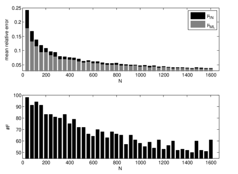
Figure 1: Comparison performance IN vs ML method. $N$ is the total number of measurements for each $(\rho_{k},\Pi_{j})$, $\mu$ is the mean relative error as introduced in (38), while $\#F$ denotes the number of failures of the IN method, i.e. the times in which the reconstructed $\chi$ is not positive.

is depicted the results obtained for different lengths $N$ of measurements related to $\{c_{jk}^{l}\}$. The mean error norm of ML method is smaller than the one corresponding to the IN method, in particular when $N$ is small (typical situation in the practice). In addition, more than half of the estimates obtained by the IN method are not positive semidefinite, i.e not physically acceptable, even when $N$ is sufficient large. Finally, we observe that for both methods the mean error decrease as $N$ grows. This fact confirms in the practice their consistency.

4.2 Minimal setting

Let $\mathcal{T}_{M,L}$ denote the set of the experimental settings with $L$ input states and $M$ observables satisfying Proposition 3.1. Accordingly the set of the minimal experimental settings is $\mathcal{T}_{d^{2}-1,d^{2}}$. Here, we consider the case $d=2$. We want to compare the performance of the minimal settings in $\mathcal{T}_{3,4}$ with those settings that employ more input states and observables. We shall do so by picking a test channel, finding a minimal setting that performs well, and comparing its performance with a non minimal setting in $\mathcal{T}_{M,L}$, $M>3,L\geq 4$ that performs well in this set while the total number $N_{T}$ of trials is fixed.

Consider the Kraus map (1) representing a perturbed amplitude damping operation ($\gamma=0.5$) with

$$K_{1}=\sqrt{0.9}\left[\begin{array}[]{cc}\sqrt{0.5}&0\\ 0&0\\ \end{array}\right],K_{2}=\sqrt{0.9}\left[\begin{array}[]{cc}1&0\\ 0&\sqrt{0.5}\\ \end{array}\right],$$

$K_{3}=\sqrt{0.1}/2I_{2}$, $K_{j}=\sqrt{0.1}/2\sigma_{l(j)}$, $j=4,5,6,$ $l(j)=x,y,z$ corresponding to the $\chi$-representation

$$\chi=\left[\begin{array}[]{cccc}0.95&0&0&0.6364\\ 0&0.5&0&0\\ 0&0&0.05&0\\ 0.6364&0&0&0.5\\ \end{array}\right].$$

We set the total number of trials $N_{T}=3600$. Fixed the set $\mathcal{T}_{M,L}$ $M\geq 3$ $L\geq 4$, we take into account the following procedure:

• Set $N=N_{T}\setminus(LM)$.

• Choose a randomly generated collection $\{\mathrm{T}_{m}\}_{m=1}^{100}$, $\mathrm{T}_{m}\in\mathcal{T}_{M,L}$.

• Perform $50$ experiments for each $\mathrm{T}_{m}$. At the $l$-th experiment we have a sample data $\{f_{jk}^{m}(l)\}$ corresponding to $\chi$ and $\mathrm{T}_{m}$. From $\{f_{jk}^{m}(l)\}$ compute the estimate $\hat{\chi}_{m}(l)$ using the ML method and the corresponding error norm $e_{m}(l)=\|\hat{\chi}_{m}(l)-\chi\|/\|\chi\|$.

• When the experiments corresponding to $\mathrm{T}_{m}$ are completed, compute the mean error norm $\mu_{m}=\frac{1}{50}\sum_{l=1}^{50}e_{m}(l)$.

• When we have $\mu_{m}$ for $m=1\ldots 100$, compute

  $$\bar{\mu}_{M,L}=\min_{m\in\{1,\ldots,100\}}\mu_{m}.$$

In Figure 2,

Figure 2: $\bar{\mu}_{M,L}$ for different values of $M$ and $L$.

$\bar{\mu}_{M,L}$ is depicted for different values of $M$ and $L$. As we can see, incrementing the number of input states/observables does not lead to an improvement in the performance index. Analogous results have been observed with other choices of test maps and $N_{T}$. Finally, in Figure 3

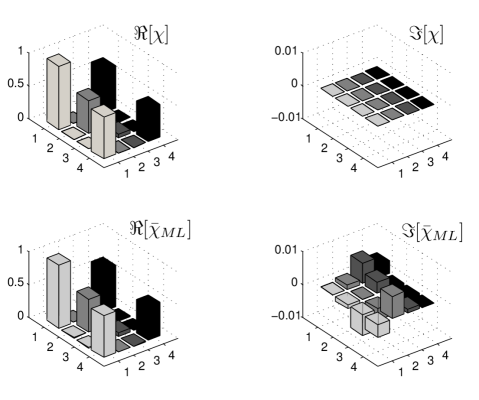
Figure 3: Real and imaginary part of $\chi$ (top) and the averaged estimation $\bar{\chi}_{ML}$ (bottom). In order to improve readability, the vertical scale of the imaginary part has been magnified in order to show the errors are below 0.01.

is depicted the true $\chi$ and the averaged estimation $\bar{\chi}_{ML}=\frac{1}{50}\sum_{l=1}^{50}\chi_{m}(l)$ with $m=\arg\min_{m\in\{1,\ldots,100\}}\mu_{m}$ for $M=3$ and $L=4$.

Appendix A Partial trace

We here briefly recall the definition and some mathematical facts about the partial trace, without reference to its fundamental use in statistical quantum theory as the way to compute reduced (marginal) states, since we do not employ it to that scope. See e.g. [29, 32] for a comprehensive discussion.

Consider two finite-dimensional vector spaces ${\mathcal{V}}\,{\mathcal{W}},$ with $\dim{\mathcal{V}}=m,\,\dim{\mathcal{W}}=n.$ Let us denote by ${\mathcal{M}}_{j}$ the set of complex matrices of dimension $j\times j.$ Let $\{M_{j}\}$ be a basis for ${\mathcal{M}}_{m},$ and $\{N_{j}\}$ be a basis for ${\mathcal{M}}_{n},$ representing linear maps on ${\mathcal{V}}$ and ${\mathcal{W}},$ respectively. Consider ${\mathcal{M}}_{mn}={\mathcal{M}}_{m}\otimes{\mathcal{M}}_{n}$: it is easy to show that the $m^{2}\times n^{2}$ linearly independent matrices $\{M_{j}\otimes N_{k}\}$ form a basis for ${\mathcal{M}}_{mn},$ where $\otimes$ denotes the Kronecker product. Thus, one can express any $X\in{\mathcal{M}}_{mn}$ as

$$X=\sum_{jk}c_{jk}M_{j}\otimes N_{k}.$$

The partial trace over ${\mathcal{W}}$ is the linear map

$$\textrm{tr}_{\mathcal{W}} : {\mathcal{M}}_{mn}\rightarrow{M}_{m}$$

$$X\mapsto\textrm{tr}_{\mathcal{W}}(X):=\sum_{j}(c_{jk}\textrm{tr}(N_{k}))M_{j}.$$

An analogous definition can be given for the partial trace over ${\mathcal{V}}.$ If the two vector spaces have the same dimension, $n=m$, we will indicate with $\textrm{tr}_{1}$ and $\textrm{tr}_{2}$ the partial traces over the first and the second spaces, respectively. The partial trace can be also implicitly defined (without reference to a specific basis) as the only linear function such that for any pair $X\in{\mathcal{M}}_{m},$ $Y\in{\mathcal{M}}_{n}$:

$$\textrm{tr}_{\mathcal{W}}(X\otimes Y)=\textrm{tr}(Y)X.$$

By linearity, this clearly implies

$$\textrm{tr}((A\otimes I)B)=\textrm{tr}(A\,\textrm{tr}_{2}(B)).$$

Notice that if $X\in{\mathcal{M}}_{mn}$, we may partition $X$ as an $m\times m$ block-matrix with block of size $n\times n$. In this way the partial trace with respect over the second space may be conveniently expressed as:

$$\textrm{tr}_{\mathcal{W}}(X) = \textrm{tr}_{\mathcal{W}}\left[\begin{array}[]{ccc}X_{11}&\dots&X_{1m}\\ \vdots&\vdots&\vdots\\ X_{m1}&\dots&X_{mm}\end{array}\right]$$

$$= \left[\begin{array}[]{ccc}\textrm{tr}(X_{11})&\dots&\textrm{tr}(X_{1m})\\ \vdots&\vdots&\vdots\\ \textrm{tr}(X_{m1})&\dots&\textrm{tr}(X_{mm})\end{array}\right].$$

The partial trace with respect to $\mathcal{V}$, $\textrm{tr}_{\mathcal{V}}(X)$, is instead the $n\times n$ matrix having in position $j,k$ the trace of the $m\times m$ matrix formed by selecting only the $(j,k)$ element of each of the blocks $X_{{\color[rgb]{0,0,0}jk}}$.

Appendix B Global convergence of the Newton algorithm

To prove the convergence of our Newton algorithm we need of the following result.

Proposition B.1

Consider a function $f:X\subset\mathbb{R}^{n}\rightarrow\mathbb{R}$ twice differentiable on $X$ with $H_{x}$ the Hessian of $f$ at $x$. Suppose moreover that $f$ is strongly convex on a set $D\subset X$, i.e. there exists a constant $m>0$ such that $H_{x}\geq mI$ for $x\in D$, and $H_{x}$ is Lipschitz continuous on $D$. Let $\{x_{i}\}\in D$ be the sequence generated by the Newton algorithm. Under these assumptions, Newton’s algorithm with backtracking converges globally. More specifically, $\{x_{i}\}$ decreases in linear way for a finite number of steps, and converges in a quadratic way to the minimum point after the linear stage.

Proof. See [12, 9.5.3, p. 488]. $\Box$ We proceed in the following way: Identify a compact set $D$ such that $\underline{\theta}_{l}\in D$ and prove that the Hessian is coercive and Lipschitz continuous on $D$. We then apply Proposition B.1 in order to prove the convergence.
Since $\underline{\theta}_{0}\in\mathop{\rm\,int}\left(\mathcal{C}\right)$ we consider the set

$$D:=\{\underline{\theta}\in\mathbb{R}^{d^{4}-d^{2}}\;|\;G_{q}(\underline{\theta})\leq G_{q}(\underline{\theta}_{0})\}.$$ (41)

The presence of the backtracking stage in the algorithm guarantees that the sequence $G_{q}(\underline{\theta}_{0}),G_{q}(\underline{\theta}_{1}),\ldots$ is decreasing. Thus $\underline{\theta}_{l}\in D$, $\forall l\geq 0$.

Proposition B.2

The following facts hold:

1. $D$ is a compact set.

2. $H_{\underline{\theta}}$ is coercive and bounded on $D$, namely there exist $s,S>0$ such that

   $$sI\leq H_{\underline{\theta}}\leq SI\hskip 28.45274pt\forall\;\underline{\theta}\in D.$$ (42)

3. $H_{\underline{\theta}}$ is Lipschitz continuous on $D$.

Proof. 1) $D$ is contained into the bounded set $\mathcal{C}$. Since $D$ is a finite dimensional space, it is sufficient to show that

$$\lim_{\underline{\theta}\rightarrow\partial\mathcal{C}}G_{q}(\underline{\theta})=+\infty.$$ (43)

Here, we have three kind of boundary: $\partial\mathcal{I}\cap\mathop{\rm\,int}\left(A_{+}\right)$, $\mathop{\rm\,int}\left(\mathcal{I}\right)\cap\partial A_{+}$ and $\partial\mathcal{I}\cap\partial A_{+}$. Notice that, $\log\det(\chi(\underline{\theta}))$ takes finite values on $\partial\mathcal{J}\cap\mathop{\rm\,int}\left(A_{+}\right)$. Accordingly, taking (21) into account,

$$\lim_{\underline{\theta}\rightarrow\partial\mathcal{I}\cap\mathop{\rm\,int}\left(A_{+}\right)}G_{q}(\underline{\theta})=q\lim_{\underline{\theta}\rightarrow\partial\mathcal{I}\cap\mathop{\rm\,int}\left(A_{+}\right)}J(\underline{\theta})=+\infty.$$ (44)

Then, $\mathop{\rm\,int}\left(\mathcal{I}\right)\cap\partial A_{+}$ is the set of $\underline{\theta}$ for which $J$ is bounded and there exists at least one eigenvalue of $\chi(\underline{\theta})$ equal to zero. Thus,

$$\lim_{\underline{\theta}\rightarrow\mathop{\rm\,int}\left(\mathcal{I}\right)\cap\partial A_{+}}G_{q}(\underline{\theta})=-\lim_{\underline{\theta}\rightarrow\mathop{\rm\,int}\left(\mathcal{I}\right)\cap\partial A_{+}}\log\det(\chi(\underline{\theta}))=+\infty.$$ (45)

Finally, from (44) and (45) it follows that $G_{q}(\underline{\theta})$ diverges as $\underline{\theta}$ approach $\partial\mathcal{I}\cap\partial A_{+}$.
2) First, observe that $D\subset\mathop{\rm\,int}\left(\mathcal{C}\right)$. Since $D$ is a compact set, there exists $s>0$ such that

$$\chi(\underline{\theta})^{-1}\geq sI\;\;\forall\;\underline{\theta}\in D.$$ (46)

Define

$$\delta_{jk}:=\frac{1-f_{jk}}{[1-\textrm{tr}(\chi(\underline{\theta})B_{jk})]^{2}}+\frac{f_{jk}}{[\textrm{tr}(\chi(\underline{\theta})B_{jk})]^{2}}>0$$

$$[M_{jk}]_{r,s}:=\textrm{tr}(Q_{r}B_{jk})\textrm{tr}(Q_{s}B_{jk})$$

where $M_{jk}$ is a positive semidefinite matrix with rank equal to one. Accordingly,

$$[H_{\underline{\theta}}]_{r,s} = q\sum_{j,k}\delta_{jk}[M_{jk}]_{r,s}+\textrm{tr}[\chi(\underline{\theta})^{-\frac{1}{2}}Q_{r}\chi(\underline{\theta})^{-1}Q_{s}\chi(\underline{\theta})^{-\frac{1}{2}}]$$

$$\geq q\sum_{j,k}\delta_{jk}[M_{jk}]_{r,s}+s\textrm{tr}[Q_{r}\chi(\underline{\theta})^{-1}Q_{s}]$$

$$\geq q\sum_{j,k}\delta_{jk}[M_{jk}]_{r,s}+s^{2}\textrm{tr}[Q_{r}Q_{s}]$$

$$\geq q\sum_{j,k}\delta_{jk}[M_{jk}]_{r,s}+s^{2}\langle Q_{r},Q_{s}\rangle.$$

Since $\{Q_{l}\}_{l=1}^{12}$ are orthonormal matrices and $\delta_{jk}M_{jk}\geq 0$, we have that

$$H_{\underline{\theta}}\geq q\sum_{j,k}\delta_{jk}M_{jk}+s^{2}I\geq s^{2}I.$$ (47)

Notice that, $H_{\underline{\theta}}$ is continuous on $\mathop{\rm\,int}\left(\mathcal{C}\right)$. Since $D\subset\mathop{\rm\,int}\left(\mathcal{C}\right)$, it follows that $H_{\underline{\theta}}$ is continuous on the compact $D$. Hence, there exists $S>0$ such that $H_{\underline{\theta}}\leq SI$ $\forall\;\underline{\theta}\in D$. We conclude that $H_{\underline{\theta}}$ is coercive and bounded on $D$.
3) $H_{\underline{\theta}}$ is continuous on $D$ and $\|H_{\underline{\theta}}\|\leq S$ $\forall\;\underline{\theta}\in D$, therefore $H_{\underline{\theta}}$ is Lipschitz continuous on $D$. $\Box$ Since all the hypothesis of the Proposition B.1 are satisfied, we have the following proposition.

Proposition B.3

The sequence $\{\underline{\theta}_{l}\}_{l\geq 0}$ generated by the Newton algorithm of Section 3.5 converges to the unique minimum point $\hat{\underline{\theta}}^{q}\in\mathop{\rm\,int}\left(\mathcal{C}\right)$ of $G_{q}$.

References

- [1] Principles and applications of control in quantum systems. Int. J. Robust Nonlinear Control, 15:647 – 667, 2005.
- [2] A. Aiello, G. Puentes, D. Voigt, and J. P. Woerdman. Maximum-likelihood estimation of mueller matrices. Opt. Lett., 31(6):817–819, 2006.
- [3] R. Alicki and K. Lendi. Quantum Dynamical Semigroups and Applications. Springer-Verlag, Berlin, 1987.
- [4] C. Altafini. Coherent control of open quantum dynamical systems. Phys. Rev. A, 70(6):062321:1–8, 2004.
- [5] C. Altafini. Feedback stabilization of isospectral control systems on complex flag manifolds: application to quantum ensembles. IEEE Trans. Aut. Contr., 11(52):2019–2028, 2007.
- [6] V. P. Belavkin. Towards the theory of control in observable quantum systems. Automatica and Remote Control, 44:178–188, 1983.
- [7] G. Benenti and G. Strini. Simple representation of quantum process tomography. Phys. Rev. A, 80(2):022318, 2009.
- [8] R. Bhatia. Matrix Analysis. Springer-Verlag, New York, 1997.
- [9] I. Bongioanni, L. Sansoni, F. Sciarrino, G. Vallone, and P. Mataloni. Experimental quantum process tomography of non-trace-preserving maps. Phys. Rev. A, 82(4):042307, 2010.
- [10] N. Boulant, T. F. Havel, M. A. Pravia, and D. G. Cory. Robust method for estimating the lindblad operators of a dissipative quantum process from measurements of the density operator at multiple time points. Phys. Rev. A, 67(4):042322:1–12, 2003.
- [11] D. Bouwmeester, A. Ekert, and A. Zeilinger, editors. The Physics of Quantum Information: Quantum Cryptography, Quantum Teleportation, Quantum Computation. Springer-Verlag, 2000.
- [12] S. Boyd and L. Vandenberghe. Convex Optimization. Cambridge University Press, Cambridge, UK, 2004.
- [13] M. Dahleh, A.Pierce, H. Rabitz, and V. Ramakrishna. Control of molecular motion. Proc. IEEE, 84:6–15, 1996.
- [14] M. Dahleh, A. Peirce, H. Rabitz, and V. Ramakrishna. Control of molecular motion. Proceedings of the IEEE, 84:7–15, 1996.
- [15] D. D’Alessandro. Introduction to Quantum Control and Dynamics. Applied Mathematics & Nonlinear Science. Chapman & Hall/CRC, 2007.
- [16] D. D’Alessandro and M. Dahleh. Optimal control of two level quantum system. IEEE Trans. Aut. Contr., 46(6):866–876, 2001.
- [17] G. M. D’Ariano, L. Maccone, and M. G. A. Paris. Quorum of observables for universal quantum estimation. Journal of Physics A: Mathematical and General, 34(1):93, 2001.
- [18] A. Doherty, J. Doyle, H. Mabuchi, K. Jacobs, and S. Habib. Robust control in the quantum domain. Proceedings of the IEEE Conference on Decision and Control, 1:949–954, 2000.
- [19] D. Dong and I.R. Petersen. Quantum control theory and applications: a survey. IET Control Theory Appl., 4(12):2651 – 2671, 2010.
- [20] J. Fiurášek and Z. Hradil. Maximum-likelihood estimation of quantum processes. Phys. Rev. A, 63(2):020101, Jan 2001.
- [21] A. Holevo. Statistical Structure of Quantum Theory. Lecture Notes in Physics; Monographs: 67. Springer-Verlag, Berlin, 2001.
- [22] R. A. Horn and C. R. Johnson. Matrix Analysis. Cambridge University Press, New York, 1990.
- [23] M.R. James, H.I. Nurdin, and I.R. Petersen. control of linear quantum stochastic systems. IEEE Trans. Aut. Contr, 53(8):1787 –1803, 2008.
- [24] N. Khaneja, R.W. Brockett, and S.J. Glaser. Time optimal control of spin systems. Phys. Rev. A., 63:032308, 2001.
- [25] P. Kosmol. Optimierung und Approximation. de Gruyter, Berlin, 1991.
- [26] K. Kraus. States, Effects, and Operations: Fundamental Notions of Quantaum Theory. Lecture notes in Physics. Springer-Verlag, Berlin, 1983.
- [27] H. Mabuchi and N. Khaneja. Principles and applications of control in quantum systems. International Journal of Robust and Nonlinear Control, 15:647 – 667, 2005.
- [28] M. Mohseni, A. T. Rezakhani, and D. A. Lidar. Quantum-process tomography: Resource analysis of different strategies. Phys. Rev. A, 77(3):032322, 2008.
- [29] M. A. Nielsen and I. L. Chuang. Quantum Computation and Information. Cambridge University Press, Cambridge, 2002.
- [30] H.I. Nurdin, M.R. James, and I.R. Petersen. Coherent quantum LQG control. Automatica, 45:1837–1846, 2009.
- [31] M. G. A. Paris and J. R̆ehác̆ek, editors. Quantum States Estimation, volume 649 of Lecture Notes Physics. Springer, Berlin Heidelberg, 2004.
- [32] D. Petz. Quantum Information Theory and Quantum Statistics. Springer Verlag, 2008.
- [33] Massimiliano F. Sacchi. Maximum-likelihood reconstruction of completely positive maps. Phys. Rev. A, 63(5):054104, Apr 2001.
- [34] F. Ticozzi and L. Viola. Analysis and synthesis of attractive quantum Markovian dynamics. Automatica, 45:2002–2009, 2009.
- [35] J. R̆ehác̆ek, B.-G. Englert, and D. Kaszlikowski. Minimal qubit tomography. Phys. Rev. A, 70(5):052321, 2004.
- [36] R. van Handel, J. K. Stockton, and H. Mabuchi. Feedback control of quantum state reduction. IEEE Trans. Aut. Contr., 50(6):768–780, 2005.
- [37] P. Villoresi, T. Jennewein, F. Tamburini, C. Bonato M. Aspelmeyer, R. Ursin, C. Pernechele, V. Luceri, G. Bianco, A. Zeilinger, and C. Barbieri. Experimental verification of the feasibility of a quantum channel between space and earth. New Journal of Physics, 10:033038, 2008.
- [38] H. M. Wiseman and G. J. Milburn. Quantum Measurement and Control. Cambridge University Press, 2009.
- [39] M. Ziman, M. Plesch, V. Bužek, and P. Štelmachovič. Process reconstruction: From unphysical to physical maps via maximum likelihood. Phys. Rev. A, 72(2):022106, 2005.