Layers of Cold Dipolar Molecules in the Harmonic Approximation

Abstract

We consider the $N$-body problem in a layered geometry containing cold polar molecules with dipole moments that are polarized perpendicular to the layers. A harmonic approximation is used to simplify the Hamiltonian and bound state properties of the two-body inter-layer dipolar potential are used to adjust this effective interaction. To model the intra-layer repulsion of the polar molecules, we introduce a repulsive inter-molecule harmonic potential and discuss how its strength can be related to the real dipolar potential. However, to explore different structures with more than one molecule in each layer, we treat the repulsive harmonic strength as an independent variable in the problem. Single chains containing one molecule in each layer, as well as multi-chain structures in many layers are discussed and their energies and radii determined. We extract the normal modes of the various systems as measures of their volatility and eventually of instability, and compare our findings to the excitations in crystals. We find modes that can be classified as either chains vibrating in phase or as layers vibrating against each other. The former correspond to acoustic and the latter to optical phonons. For the acoustic modes, our model predicts a smaller sound speed than one would naively get from expansion of the dipolar potential to second order around the origin. Instabilities can occur for large intra-layer repulsion and produce diverging amplitudes of molecules in the outer layers, and our model predicts how the breakup takes places. Lastly, we consider experimentally relevant regimes to observe the structures. The harmonic model considerd here predicts that for the multi-layer systems under current study chains with one molecule in each layer are always bound whereas two chains comprised of two molecules in each layer will not be bound. However, since realistic systems have external confinement prevention the molecules from escaping to infinity, we still expect the unstable modes to show up as resonances in the dynamics.

1 Introduction

The experimental study of cold dipolar molecules is a rapidly accelerating field dipoleexp1 ; dipoleexp2 ; dipoleexp3 ; dipoleexp4 ; dipoleexp5 ; dipoleexp6 ; ni2010 ; ospelkaus2010 ; carr2009 ; miranda2011 . The long-range anisotropic forces of polar molecules can be controlled by external alignment and tuned to be both repulsive and attractive depending on the geometric setup, which has lead to a significant amount of interesting theoretical proposals tr1 ; tr2 . In particular, stacks of thin layers containing polarized molecules interacting via dipole-dipole potentials have been suggested 2dt1 ; 2dt2 ; 2dt3 ; 2dt4 ; wang2006 as a way to control the losses that can severely influence three-dimensional experiments with strong dipolar forces ni2010 ; ospelkaus2010 ; lushnikov2002 ; micheli2010 . The layered structure and the long-range nature of the interactions holds promise for the realization of interesting few- fewbody1 ; fewbody2 ; fewbody3 ; fewbody4 ; fewbody5 ; cremon2010 ; armstrong2010 ; artem2011-1 ; artem2011-2 ; zinner2011a and many-body states mb1 ; mb2 ; mb3 ; mb4 ; mb5 ; mb6 ; mb7 ; mb8 ; mb9 ; mb10 ; mb11 ; mb12 . Recently, a stack of layers have been realized with fermionic polar ⁴⁰K⁸⁷Rb molecules miranda2011 and further cooling should produce some of the novel phases that have been proposed.

An interesting question to pose for layered systems of dipolar molecules is related to their tendency for crystallization when the dipole moment becomes large. This phenomena is similar to the famous Wigner crystal phase of the electron gas wigner1934-1 ; wigner1934-2 . However, whereas the electron gas crystallizes at low density where the Coulomb interaction dominates, a system of dipoles will crystallize at high density where the kinetic energy is negligible compared to the dipole force. In a single two-dimensional (2D) layer with dipoles oriented perpendicular to the layer this has been studied in classical simulations kalia1981-1 ; kalia1981-2 , and more recently in quantum Monte Carlo simulations dc1 ; dc2 ; dc3 , and for large dipole moments evidence for a triangular crystal structure is found. Studies in one-dimensional (1D) dipolar systems also find interesting crystal phases 1dc1 ; 1dc2 ; 1dc3 ; 1dc4 ; 1dc5 ; 1dc6 ; 1dc7 ; 1dc8 which are similar to those seen in ion Coulomb crystals fishman2008-1 ; fishman2008-2 . Crystal phases have also been found in 2D with an in-plane optical lattice for arbitrary polarization quin2009-1 ; quin2009-2 .

Here we are interested in the case of a multi-layer system with dipoles perpendicular to the planes as in recent experiments miranda2011 . The possibility of having bound states consisting of chains with one molecule in each layer has been discussed for both bosonic wang2006 ; wang2008a and fermionic molecules santos2010 . In the limit of large dipole moments, a study of the two-layer (bilayer) case using classical dynamics showed that the triangular crystals appear spatially correlated, i.e. the molecules in the crystal lattice sit on top of each other lu2008 . This is also the expected behaviour for more than two layers and we note that a recent quantum Monte Carlo study finds evidence of a transition to rough chains for bosonic molecules at a critical dipole strength barbara2011 .

In the present work we consider strongly interacting distinguishable dipolar molecules before they enter the crystal phase. Rather than fixing the position of the molecules to a particular lattice and calculate fluctuations about this state, we consider an $N$-body system with a fixed number of molecules in each layer and study the quantum spectrum to obtain information about the modes of the system before it crystallizes. Most of the studies on multi-layer systems mentioned above are based in one way or another on a harmonic approximation to the interaction potential which renders the otherwise intractable $N$-body problem solvable in certain limits, and provides ground state and excitation modes of the system. In this paper we also make use of the harmonic approximation to derive a solvable $N$-body problem. However, we go beyond previous studies in two important aspects; i) we use the two-body binding energy to fix the interlayer attractive interactions for the effective harmonic hamiltonian and ii) we include parametrically the repulsive interaction between molecules in the same layer which has been neglected thus far except in the classical calculations of Ref. lu2008 .

To arrive at our effective harmonic Hamiltonian, we use the method recently formulated in Refs. armstrong2010 ; armstrong2011 . We proceed in two steps, that is first the one- and two-body interactions are approximated by quadratic forms, and second the resulting $N$-body Schrödinger equation is solved exactly. We replace the true interactions with quadratic forms in the molecule coordinates, either by direct fits of the potentials or by adjusting parameters to reproduce crucial properties. This approximation allows analytical investigations of the $N$-body system with the properties expressed in terms of the two-body characteristics.

The harmonic model studied here predicts that chains with a single molecule are stable for any interaction strength. A complex with two molecules in each layer, i.e. two chains in close proximity, will most likely not be bound as we estimate the critical strength for breakup to be below the strength in current experimental setups. However, experiments are always performed in the presence of an external confinement and we expect the unstable modes of complexes with multiple chains to appear as resonances. We therefore study the modes as function of the intralayer repulsion to determine how the system breaks into single chains and elucidate its structure.

The paper is organized as follows. In Section 2 we describe the harmonic approximation method used and Section 3 discusses in detail the chain structure with one molecule in each layer. This involves energies, radii, and normal mode excitations. Section 4 deals with multiple chains and layers with many molecules. The intralayer repulsion is taken as a parameter in the harmonic approximation. The normal modes reveal the most likely decay mechanism, and extract configurations of the most unstable degrees of freedom. In particular, we calculate the critical stability properties of the system and discuss how the system breaks up into smaller structures. In Section 5 we discuss how the intralayer repulsion influences the system size and densities, and we discuss relative energies of the many-body systems. Finally, Section 6 contains summary and conclusions.

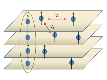
Figure 1: Pictorial view of the multi-layered system containing dipolar molecules. The attractive interlayer ($V_{a}$) and repulsive intralayer ($V_{r}$) are illustrated, along with a potential bound chain state containing four molecules.

2 Method

We consider a system of $N$ dipolar molecules of mass, $m$, and dipole moment, $D$, distributed in a series of parallel two-dimensional layers separated by a distance $d$ as illustrated in figure 1. The planar coordinates of the k’th molecule are $(x_{k},y_{k})$. The dipoles are oriented perpendicular to the layers and the molecules interact pairwise through the dipole-dipole potential, $V$, which in different planes is given as

$$V(x,y,n)=D^{2}\frac{x^{2}+y^{2}-2(nd)^{2}}{(x^{2}+y^{2}+(nd)^{2})^{5/2}},$$ (1)

where $n$ is the number of layers separating the two molecules, and $(x,y)$ are the relative coordinates of the two molecules. We define the dimensionless strength, $U=mD^{2}/(\hbar^{2}d)$. For $n=1$ we have a nearest neighbour interaction, for $n=2$ a next-nearest neighbour interaction and so forth. Below we will also use the standard notation for the radius $r=\sqrt{x^{2}+y^{2}}$. Molecules in the same layer repel each other and if identical are also subject to (anti)symmetrization conditions for fermions and bosons. Here we will ignore symmetry considerations and consider our molecules distinguishable. Since we work in the strongly-coupled regime and we do not expect the chains to have large overlap this is a reasonable assumption. The Hamiltonian for the $N$-body system is then

$$H=-\frac{\hbar^{2}}{2m}\sum_{k=1}^{N}\left(\frac{\partial^{2}}{\partial x_{k}^{2}}+\frac{\partial^{2}}{\partial y_{k}^{2}}\right)+\frac{1}{2}\sum_{i\neq k}V(x_{ik},y_{ik},n_{ik}),$$ (2)

where $(x_{ik},y_{ik})=(x_{i}-x_{k},y_{i}-y_{k})$, and $V$ for different layers is from equation (1) or the corresponding repulsion for molecules in the same layer. This $N$-body Hamiltonian is solved using the method described in Ref. armstrong2011 . Note that there is no external trapping potential in any of the planes. The $N$-body structures we consider are self-bound, i.e. they are held together by the attractive interactions between the layers. For configurations that have more than one molecules in a single layer, the attractive forces will have to overcome the repulsive intra-layer interactions. This will be disucssed in great detail later and will give raise to critical values of this intra-layer repulsion above which there are no bound structures.

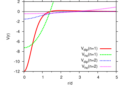
Figure 2: Potential energy curves for the nearest neighbour dipole-dipole interaction ($V_{dip}(n=1)$) and the harmonic oscillator potential ($V_{ho}(n=1)$) with the same binding energy. The next-nearest neighbour dipole-dipole interaction is also shown ($V_{dip}(n=2)$) as well as the oscillator potential with the matching binding energy ($V_{ho}(n=2)$). The dipole strength is here chosen as $U=6$. The resulting binding energies are $B_{2}=3.44$ and $0.20$ in units of $\hbar^{2}/md^{2}$.

To render properties of systems with $N$ molecules analytically tractable, we simulate the effects of the dipole-dipole interaction by harmonic oscillator potentials as described in armstrong2011 . We replace the actual interaction in equation (1) with a shifted harmonic oscillator, $V_{ho}$, which has its node in the same place as the dipole-dipole potential, i.e.,

$$V_{ho}(x,y,n)=V_{0}\left(\frac{x^{2}+y^{2}}{2(nd)^{2}}-1\right).$$ (3)

The potentials in equations (1) and (3) are negative (and positive) in the same regions, and have nodes in the same places, see figure 2. The strength, $V_{0}$, is finally adjusted to reproduce the two-body dipole-dipole binding energy. This means that $V_{0}$ is a specific function of the dipole moment, the molecule mass, and distance between the layers, $V_{0}(D^{2},m,d)$ The corresponding oscillator frequency, $\omega_{a}$, is then given by

$$\omega_{a}^{2}=\frac{2V_{0}(D^{2},m,d)}{m(nd)^{2}}\;,$$ (4)

where the reduced mass of the two-body system is $m/2$.

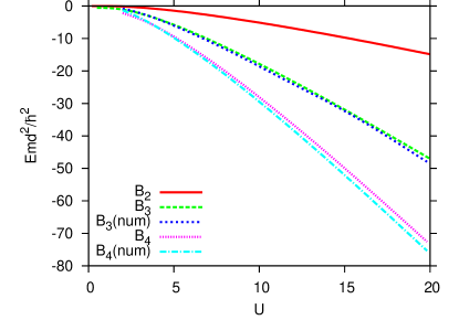
Figure 3: Binding energies for two, $B_{2}$, three $B_{3}$, and four $B_{4}$ molecules as functions of strength, $U=mD^{2}/\hbar^{2}d$, of the dipole potential. The oscillator approximation (solid, red) and the accurate numerical calculation (dashed, blue) are compared for three ($B_{3}(\text{num})$) and four molecules ($B_{4}(\text{num})$). The numerical calculations are courtesy of A. G. Volosniev using the method described in artem2011-1 ; artem2011-2 .

The key ingredient is here the two-body binding energy, $B_{2}$, which from equation (2) for two molecules is seen to scale with layer distance, $nd$, as

$$B_{2}(n)=\frac{\hbar^{2}}{m(nd)^{2}}f\bigg{(}\frac{mD^{2}}{nd\hbar^{2}}\bigg{)}\;,$$ (5)

where $f$ is a universal function. For $n=1$, that is, for neighbouring layers, we show $B_{2}$ in figure 3 as function of potential strength, $D^{2}$. The two-body interaction for pairs of molecules in layers separated by the distance, $nd$, is then obtained through the scaling in equation (5). Upon comparing the root-mean-square radius of the exact solution to the oscillator approximation one finds very good agreement for $U\gtrsim 2$ which is also where the binding energy of the exact and harmonic approximation for two molecules are very close armstrong2011 ; zinner2011a .

These energies are then the crucial input in the $N$-body calculations. At small strength the approach to zero is extremely strong artem2011-1 ; artem2011-2 whereas at larger strengths the behaviour is smooth and in a region almost linear in $U$. We need two-body interactions between each pair, the most important being between adjacent layers at a distance $d$. For larger than one-layer separations the potential becomes increasingly more shallow, flat and spatially extended, see figure 2. The scaling of $B_{2}$ with layer number is $n^{-2}$ computed for a strength $U/n$ (see equation (5)).

This procedure of adjusting strengths for different shapes of potentials to get the same binding energy has proved efficient in other contexts where effective interactions are used. The method is frequently applied in dripline nuclear physics, where knowledge about the systems can be limited to an energy of one bound state, or resonance jen04 . It is also the philosophy employed for cold atoms where the scattering length is used as the parameter characterizing a short-range two-body interaction, and subsequently used in $N$-body calculations. However, the dipolar interaction is long-ranged. In fact, for typical experimental densities, the range of the dipole-dipole forces is comparable to the inter-particle distance. This implies that one should take more than just the zero-energy properties into account.

The accuracy of the procedure is tested by comparing the oscillator approximation with numerical calculations of the energies of three and four molecules with one in each layer using a method similar to the one described in artem2011-1 ; artem2011-2 , see figure 3. The remarkable precision of the oscillator results for three molecules is reassuring in the applications on $N$ molecules.

We note that the procedure used here to fix the frequency of the attractive interlayer interaction is naturally very different from expanding the potential in equation (1) for $r/d\ll 1$ to get the harmonic term zinner2011a . We include more accurately the two-body properties into the $N$-body system and expect therefore to provide a better approximation for the dynamics of a single chain and also for the interaction of several chains as we discuss below.

2.1 Repulsive In-Plane Interactions

Two polar molecules in the same layer repel each other when both dipoles are perpendicular to the plane. This repulsive intralayer interaction scales with the dipole strength similarly to the attractive interlayer dipolar interaction. Within the framework of effective harmonic hamiltonian we would like to replace the real intralayer potential by something that can model a repulsion, which can be achieved by using an inverted oscillator. The repulsive interaction is therefore replaced by a term of the form

$$V_{rep}(x,y)=-\frac{1}{4}m\omega_{r}^{2}\left(x^{2}+y^{2}\right)+V_{r0},$$ (6)

where $1/4$ arise from use of the reduced mass, $\omega_{r}$ is the corresponding frequency, and $V_{r0}$ is a constant shift. This inverted oscillator favors a large (infinite) distance between the molecules, and acts consequently as a repulsion. The shift is parametrized as

$$V_{r0}=\frac{1}{4}m\alpha^{2}\omega_{r}^{2}d^{2},$$ (7)

where we use $d$ as the natural length, and leave the dimensionless scale factor, $\alpha$, for later adjustment. The distance where the potential changes sign is then $r=\alpha d$.

We will demonstrate below that the inverted oscillator provides us with a parametrically sound way of including repulsive forces in our model. That is, it provides a handle on the effect of repulsion in the detailed balance between repulsively and attractively interacting pairs of molecules. Therefore we are able to consider various properties of several chains in multiple layers which is one of the goals of this work.

At this point we must caution that one might naively try to fit the frequency of the repulsive term above to the true intralayer dipole interaction which has the form $V(r)=\lambda/r^{3}$. Here we introduce the dipolar strength $\lambda$ since we want to separate it from the strength of the attractive interlayer potential (1) for later discussion. If we have a system at a certain density, $n$, then the characteristic energy of the true repulsion can be estimated as $\lambda n^{3/2}$. The energy scale of an oscillator is usually $\hbar\omega_{r}$ and we then arrive at

$$\frac{md^{2}\omega_{r}}{\hbar}=\frac{m\lambda}{\hbar^{2}d}(nd^{2})^{3/2}.$$ (8)

For current experiments miranda2011 with $m\lambda/\hbar^{2}d\sim 0.1$ and $nd^{2}\sim 1$, this gives a very small contribution from the repulsive term. However, the procedure of harmonic approximation breaks down for small $U$ and/or $\lambda$, and both the attractive and repulsive parts of the potential cannot be modelled by an oscillator in this limit. Only in the limit of large $U$ does the approximation become valid for the single-chain structures as shown above. Quantitatively, we expect that harmonic oscillator wave functions are reliable for $U\gtrsim 2$ armstrong2010 ; zinner2011a . Below this value, the binding energy decreases rapidly and the state becomes extended artem2011-1 ; artem2011-2 .

As will be shown below, there are critical values of $\omega_{r}(U)$ above which the system becomes unstable as indicated by the normal mode frequencies that become imaginary. If we take densities $nd^{2}\sim 1$, the $\omega_{r}$ given by equation (8) is always larger than the critical frequency and the system is unstable. Furthermore, the densities we calculate below for the system are much larger than $nd^{2}=1$, so this gives an apparent inconsistency.

There are, however, two major points that invalidate the identification in equation (8). First, there is no zero-point energy scale for an inverted oscillator, and using $\hbar\omega_{r}$ as such is meaningless. One might attempt to make sure that the force (gradient of the potential) of the true potential and the inverted oscillator match in a region around zero, but this suffers from the same inconsistencies. The second, and more important objection, is that we must choose the repulsion in a manner that is consistent with the philosophy of using effective harmonic approximations already employed for the attractive interlayer interaction discussed above. There we really use the knowledge of two-body states in the system to fix a potential that reproduces features such as energy and potential shape.

In order to apply our philosophy, we can compare to small systems that have the effect of the repulsion included, but which can be solved by other means. The obvious choice is the four-body state with two molecules in each of two layers or two molecules in one layer and one molecule in each of the two adjacent layers in a setup with three layers. We could then compare the energetics and fit the strength of the repulsive term. Exact results on these configurations have been reported very recently in Ref. artem2011c . These results indicate that such systems are actually unstable for a critical intralayer repulsion that is much smaller than the situation where attraction and repulsion have the same value ($U=\lambda$ below). Ref. artem2011c also find that longer chains (five layers or more) could bind extra molecules as long as the additional ones are not in adjacent layers. This hints at a competition between attractive and repulsive interaction terms that is conveniently described within the harmonic oscillator approach as we demonstrate below. The results of Ref. artem2011c are, however, difficult to use as a fit for the repulsive frequency in the harmonic model due to the instability of the states. We therefore follow a different line of argument which relates the number of bound states in the (inverted) repulsive potentials as we now explain.

In a single plane, the pure inverse cubic dipolar repulsion obviously has no two-body bound states. However, if we introduce an external trapping potential, i.e. an external oscillator to keep the molecules confined, then the two-body spectrum would be shifted upward due to the repulsion. One could then imagine adding a repulsive oscillator term to fix the two parameters of the potential in (6) so that, say, the two lowest bound state energies match (or the ground state and the root-mean-square radius). Unfortunately, the results of such a procedure depend strongly on the choice of external oscillator potential. If one relates this external confinement to the density of particles in the layer (in a manner similar to (8)), then we are left with a two-body interaction that depends on the properties of the entire system. We consider this situation extremely inconvenient. This dependence of two-body physics on the many-body problem is also inherent in the naive estimate in (8).

What can be done instead, is to consider the number of bound states that the inverse dipolar potential, i.e. an attractive potential, allows and compare this to $-V_{rep}$ (6) (a normal oscillator that is shifted below zero at the origin). We consider only those bound states that have negative energy even though the shifted normal oscillator will of course have the usual ladder spectrum of states. This explains the upper limit in (11) below. We are interested in the stability of structures with several molecules in each layer, and therefore we need only require that the repulsion be reproduced within the range where there is an attraction to particles in other layers. This means that the shift term in (7) should ensure that the inverted oscillator crosses zero along the outer repulsive barrier of (1). This is roughly in the region $\sqrt{2}\leq\alpha\leq 2\sqrt{2}$ (the upper bound being defined as the point at which the repulsion of (1) is only 1% of its attractive value at the origin). The parameter $\alpha$ is therefore still somewhat arbitrary although we will compute a suitable value based on the energetics of barely stable configurations of molecules in section 5.

In a realistic setup, the layers have finite width, $w$, and therefore the $1/r^{3}$ repulsion is modified at small distances cremon2010 and attains a logarithmic dependence on relative distance of two molecules. The crossover happens for distances of order the layer width (typically $w\sim 0.1d-0.2d$ in experiments). Matching at $w$, we have

$$V_{dip}(r)=\left\{\begin{matrix}\frac{\lambda}{r^{3}}&,&r>w\\ -3\frac{\lambda}{w^{3}}\ln\left(\frac{r}{we^{1/3}}\right)&,&r<w\end{matrix}\right..$$ (9)

An estimate for the number of bound states in a two-dimensional potential can be found by integrating the (absolute value of the) negative part of the potential over space khuri2002 . For the dipolar potential we find

$$\int_{0}^{\infty}V_{dip}(r)r\,dr=\frac{9}{4}\frac{\lambda}{w},$$ (10)

while for the oscillator of (6) we find

$$\int_{0}^{\alpha d}V_{rep}(r)r\,dr=\frac{1}{16}m\omega_{r}^{2}d^{4}\alpha^{4}.$$ (11)

If we equate these expressions we obtain a relation between the repulsive frequency, $\omega_{r}$, and the parameters $\lambda$, $\alpha$, and $w$, which reads

$$\frac{md^{2}}{\hbar}\omega_{r}=\frac{6}{\alpha^{2}}\sqrt{\frac{d}{w}}\sqrt{\frac{m\lambda}{\hbar^{2}d}},$$ (12)

in dimensionless form. What we have done here is to use the number of bound states of the inverted potentials, which implies that we have in fact matched the number of bound states excluded by the presence of the repulsion. This is in similar spirit to the proposal of introducing an external oscillator discussed above. However, we avoid a dependence on properties beyond two-body physics.

In section 4 we calculate critical values of $\omega_{r}$ beyond which configuration with several molecules in each layer become unstable and break into smaller complexes. The critical repulsive frequencies we find below are $md^{2}\omega_{r}/\hbar\sim 1-10$. Taking the specific case where $m\lambda/\hbar^{2}d=20$, we find $md^{2}\omega_{r}/\hbar=7.78$. From (12) with $w=0.2d$ and $\alpha^{2}=2$, we find a larger value of $md^{2}\omega_{r}/\hbar=30$. This implies that we are in the unstable regime. However, we note that the parameter $\alpha$ is geometrical and somewhat arbitrary, constrained only by our desire to describe the competition of repulsive and attractive terms in the system. Our calculations below indicate that a better value is $\alpha\sim 1.92$. This yields $md^{2}\omega_{r}/\hbar\sim 16$, which is closer to the critical frequency.

We are thus in a situation where structures containing more than one molecule in a single layer are most likely unstable in realistic experiments. This is consistent with the conclusion of Ref. artem2011c about the instability small complexes. However, as noted above the experiments have external confinement and the structures obtained for multiple chains below the critical frequency in later section could therefore appear as resonances in the confined system. The energetics and the path to breakup for these systems is therefore an interesting question nonetheless. With a harmonic model we can study such questions for large number of particles in an essentially exact manner, given the necessary approximation on the interaction terms.

In making a distinction between $m\lambda/\hbar^{2}d$ and $U$ (from the interlayer potential (1)), we also leave open the possibility of working with more than one type of molecule or populating different internal rotational states of the molecules in different layers, both of which can modify the dipolar moment and potentially bind the structures we study here by reducing the overall repulsion. This could possibly be achieved by externally applied electromagnetic fields and lasers giovanazzi2002 ; micheli2007 ; gorshkov2008 . However, in the present study we will always assume that $\lambda=U$ and use just $U$ as the dipolar strength parameter. In light of the extended discussion above, we apply repulsive intralayer interaction parametrically through the inverted oscillator to study the effects of inter-chain interaction for the purpose of the present work.

The oscillator potential is now defined for two molecules either in different layers or the same layer. If a confinement is needed it is straightforward to add and include a one-body harmonic oscillator potential. Without a one-body external potential the relative motion separates from the free motion of the center of mass which therefore becomes uninteresting. We shall therefore consider only the relative motion.

3 One molecule per layer

The simplest many-body structure is found when only one molecule is placed in each layer. This means that all the two-body interactions are attractive and given in equation (1), and the repulsion in equation (6) is not present. Any pair of these molecules would then form a bound state as shown previously armstrong2011 ; artem2011-1 ; artem2011-2 . When the layers are far apart the potential is very shallow and the attractive part extends to a distance, $r=nd\sqrt{2}$, proportional to the distance between the layers. The attraction decreases with the third power of the layer distance, and the binding energy decreases correspondingly. Therefore the interactions dominate between the nearest neighbours.

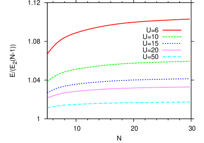
Figure 4: Energies divided by two-body energy obtained with the potential in equation (1) times number of pairs of nearest neighbours for several different dipole strengths. These energies were obtained by restricting the potential to nearest neighbours only.

3.1 Binding energies and radii

The energies could be expected to be proportional to the two-body energy, $B_{2}$, and linear in the number of interacting neighbours pairs, $N-1$. This was conjectured and estimated for large $N$ in armstrong2011 , i.e.

$$\frac{B_{N}}{(N-1)B_{2}}\approx\sum_{1}^{\infty}\frac{1}{n^{2}}=\frac{\pi^{2}}{6}\approx 1.645\;.$$ (13)

However, the assumptions are then that the interactions decrease as $1/n^{2}$, and that no additional correlations arise from the string of molecules. A better estimate should then be

$$\frac{B_{N}}{(N-1)B_{2}}\approx\sum_{1}^{\infty}\frac{1}{n^{3}}=\zeta(3)\approx 1.202\;,$$ (14)

where the first two powers are from the $d^{2}$-dependence and one power is from the reduction of interaction strength, see equation (5). The latter is an upper limit since the energy curve in figure 3 is concave. With only nearest neighbour interactions we get the energies shown in figure 4 for different dipole strengths. The variation is largest for small $N$ while the energy per interacting pair is leveling out for large $N$. All curves are between $1$ and $1.12$ with a monotonous decrease with interaction strength. Thus correlations always contribute on less than the $10\%$ level, and increase as the system becomes spatially more extended and dilute.

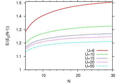
Figure 5: Energies divided by two-body energy obtained with the potential in equation (1) times number of pairs of nearest neighbours for several different dipole strengths.

Inclusion of all interactions give the energies shown in figure 5. The trends are the same with increase as function of $N$ and decrease as function of interaction strength. However, the actual values are now all between $1$ and $1.6$. The large-$N$ asymptotics seems all to be above $1.202$ indicating additional contributions from correlations which seems to approach zero in the limit of strong interactions.

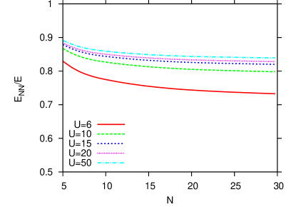
Figure 6: Energies in Fig 4 divided by the energies in figure 5, which is the fraction of the total energy of the $N$-molecule string captured by the interaction of nearest neighbours as a function of chain length for several different dipole strengths.

The 20-50% difference between energies in Figs. 4 and 5 is due to nearest neighbour and inclusion of all contributions to the energy. The corresponding fraction is directly shown in figure 6 where the trend is decrease of nearest neighbour contribution with $N$ and increase with interaction strength. Again the strongest variation is for small $N$ while asymptotic constant ratios are approached for large $N$. All ratios are between $0.7$ and $0.9$, showing how good an approximation only nearest neighbours would be, depending on strength and molecule number. The total number of interaction terms, $(N-1)^{2}/2$, increase compared to the number, $N-1$, of nearest neighbour terms. However, the rather strong fall off of the interaction with distance leads to the relatively small values in figure 6. Even when a chain gets longer, only the very nearest links in the chain are affected, and constant ratios are approached.

The approximately linear dependence of energy on $N$ implies that the separation energy, $B_{N-1}-B_{N}\propto B_{2}$, where the proportionality constant crudely can be approximated by $\zeta(3)=1.202$ (equation (14)) for large $N$ and not too weak interactions. The variation with $N$ of the separation energies is around $0.2$ for all strengths. The correlations therefore change smoothly with the number of molecules.

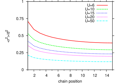
Figure 7: Radius-squared as a function of the position in the chain of 30 molecules. Position one is the outermost position of the chain, and the radii are symmetric with respect to the center of the chain, so showing only the first half of the chain is necessary.

The wave functions for each of the states are also available. They are essentially products of Gaussians of linear combinations of molecule coordinates. To get an idea of the structure, we computed mean square radii of the individual molecules measured from the common (projected) center of mass of all molecules. These radii are shown in figure 7 for a system of 30 molecules distributed in 30 layers as function of the number of layers. The molecules in the outer layers have largest radii intuitively correlated with the fewer efficiently interacting neighbours. Towards the central layer, the radii decrease and become almost independent of layer position. The radii decrease with the strength of the interaction in agreement with the smaller binding energies. This is consistent with the variational study in Ref. wang2006 .

The absolute sizes are on average between $0.3d$ and $0.9d$ for the strengths in figure 7. Clearly $d$ is the natural unit since that is the extension of the potential within each of the layers. When a radius is smaller than $d$ it means that the molecule mostly is located inside the attractive well from the nearest neighbour.

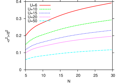
Figure 8: Radius-squared of the central molecule in a chain of length $N$ as a function of chain length for several different dipole strengths.

To see how the radii evolve with molecule number, we show the central radius as a function of molecule number in figure 8. For the same interaction strength, the size increases with molecule number. The outermost molecules are always the largest, as they only have the influence of one nearest neighbour. The size of the outermost molecule also grows slightly faster than the central molecules.

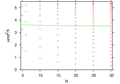
Figure 9: Normal mode frequencies (points) as a function of molecule number for a dipole strength $U=6$. The line is the average value of the frequency at a given number of molecules.

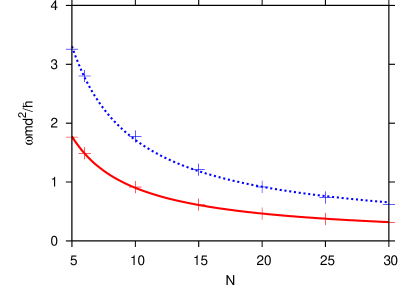
Figure 10: Normal mode frequencies (points) as a function of number of molecules $N$ along with their fits to an $A/N+B$ curve, where $A$ and $B$ are fitting parameters for a dipole strength $U=6$.

3.2 Normal excitation modes

The harmonic oscillator solutions provide a series of frequencies after the total separation of coordinates. They describe which modes are easiest to excite. For $N$ molecules we always find $N-1$ frequencies related to relative motion (some of which can be degenerate), and one degree of freedom corresponding to the trivial free center of mass motion. Note that we consider the limit where the layer is in the strict 2D limit, i.e. zero width. This means that all modes are transverse. In a real experiment with a finite width, longitudinal modes are also possible but usually have higher excitation frequencies (in the 1D case this has been discussed in Ref. astra2009 ).

In figure 9, we demonstrate how the normal modes change with chain length for a given interaction strength. As the number of molecules is increased, additional frequencies appear. When adding one molecule to a system of $N$ molecules, the $N-1$ frequencies from this $N$-molecule system all decrease in magnitude. The new additional frequency comes in above all the other frequencies, in such a way that the average frequency decreases overall. The average frequency multiplied by $N-1$ is in fact the ground state energy of the $N$-body system, except for the correction from the shift in equation (4), which to be precise should be multiplied by the number of interacting pairs. This is indicated by the horizontal line in figure 9.

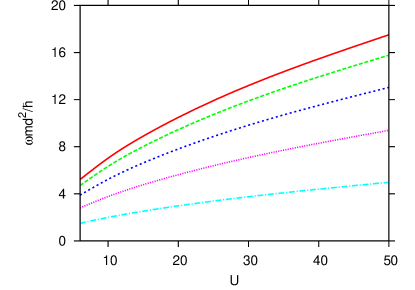
Figure 11: Frequencies of the six-molecule system as a function of dipole strength. The different lines connect frequencies of the same normal mode at different dipole strengths.

The normal modes in Fig 9 are similar to the acoustic branch modes in a crystal with a single atom in the basis. In typical textbook presentations of acoustic phonons, nearest neighbour interactions are taken into account and the spectrum has the form $\omega(k)^{2}=\tfrac{4K}{m}\sin(\tfrac{kd}{2})$, where $K$ is the harmonic force constant of Hooke’s law. Taking the naive harmonic approximation to the dipolar potential (obtained by expanding equation (1) to second order in $r/d$), we obtain $K=12D^{2}/d^{5}$. The speed of sound then becomes $c_{0}=\sqrt{\tfrac{12D^{2}}{md^{3}}}$ as discussed in Ref. wang2008a . By fitting the lowest modes of the chain as function of the chain length, we can get an estimate of the speed of sound in the harmonic framework used here.

The possible wave vector in a string of length $Nd$ is $k=n\pi/Nd$, where $n$ is an integer $n>0$. We can now use the fit in figure 10 to obtain the speed of sound and we find $c=c_{0}/3.05$, a reduction by a factor of around three. The first obvious reason for the difference is that we have taken not only nearest neighbour interactions but all interactions into account in our model. However, as we saw in relation to the energetics, the terms beyond nearest neighbour play a minor role which was also noted in Ref. wang2008a . The main difference is that the effective oscillator potential used here allows molecules to spread further in space, it is in a sense more shallow than the naive approximation around $r/d\ll 1$. This results in a less rigid string with smaller tension and therefore a reduction in the speed of sound. However, from the energetics alone it seems clear that this is a much better approximation, and we have thus shown that also the single-chain modes should be re-evaluated. Notice also that in the naive approach, $\omega(k)^{2}$ scales with $U$, whereas we find a scaling that is softer ($U^{\alpha}$ with $0<\alpha<1$) due to the reduced oscillator frequency.

The tension of the chains/strings is directly related to the average radius $\langle r^{2}\rangle$ of the particular potential used since this indicates the strength of the interaction and how fast the chain returns to its equilibrium position after a disturbance. As shown in Ref. zinner2011a , the real potential has $\langle r^{2}\rangle$ slightly smaller than the harmonic approximation used here. The naive harmonic approach has $\langle r^{2}\rangle$ that is an order of magnitude smaller than both the real potential and the effective harmonic potential used here. This is another indication that the spectrum produced here is a significant improvement over the naive approach. Based on the fact that the real dipole potential has slightly lower $\langle r^{2}\rangle$, the true speed of sound should also be somewhat higher than our estimate.

In figure 11 we show how the dipole strength affects the normal mode frequencies. They all increase, as an increase of the dipole strength essentially makes the chain stiffer. On the other hand, the curves in figure 11 are not parallel, and the frequencies diverge away from each other. The higher the frequency of the mode, the more it grows with increasing dipole strength. This is different from the usual model of acoustic phonons with only nearest neighbours, and is due to the inclusion of next-nearest neighbours and so on. The latter interactions tend to suppress short wave length modes.

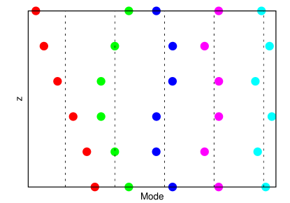
Figure 12: Normal modes for a chain with six molecules and $U=10$. The vertical axis shows the molecule’s layer position. In the horizontal direction, the modes are arranged in increasing order of frequency (not to scale). The dashed vertical line shows the equilibrium position of the molecules, which are shown as points. The frequencies of the modes are, from left to right, 2.00, 3.77, 5.23, 6.34, and 7.03 in units of $\hbar/(md^{2})$.

The structure of the normal mode excitations are displayed in figure 12 for a chain of six molecules. We show the maximum displacement amplitudes in one direction of the 2D structures. The lowest energy mode has one node in the vibration of the string, the next mode has two nodes, and so forth. This ordering remains for all dipole strengths, and the amplitudes of the molecules change very little.

It should be noted that this pictorial representation is in one dimension. The other direction is degenerate but independent, which implies that linear combinations of each of these one-dimensional modes are equally appropriate. The displacements could happen along any two independent directions in the $xy$-plane. This is reflected in the fact that we always find two degenerate modes for each normal mode frequency, both for single chains and for several chains per layer as discussed below. For example, we could choose a radial and tangential mode in the planes instead of the Cartesian one-dimensional modes illustrated in figure 12. Still they would have to present nodes at the same layers, where the molecules remain at their equilibrium position.

4 Multiple chains and layers

Molecules in different layers still attract each other as parametrized in equation (3). However, more than one molecule in the same layer immediately introduces the repulsion between these molecules. We parametrize this additional interaction in equation (6) where we treat the repulsive frequency, $\omega_{r}$, as a free parameter. All structure calculations are independent of the constant shift which only enters in energy calculations. We therefore first discuss structure variation as $\omega_{r}$ is increased from zero. Eventually there is a point when the repulsion is too strong compared to the inter-layer attraction, and the system is no longer bound. This is seen as at least one imaginary normal mode frequency solution to the full $N$-body problem.

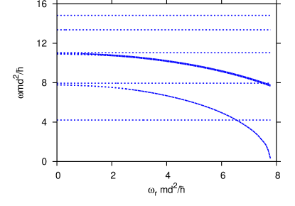
Figure 13: Evolution of the normal mode frequencies as a function of the intra-layer repulsive frequency, $\omega_{r}$. The modes are for two strings of six molecules with $U=20$.

4.1 Energies and repulsion

We now solve for $N$ layers and two dipolar molecules in each layer. The resulting frequencies are shown in figure 13 for $N=6$ as function of the repulsive frequency. There are $11$ normal mode frequencies for these $12$ molecules, one mode is related to the free center of mass motion. Five of these modes do not depend on the repulsive frequency. They correspond to the modes of the singly occupied layers (similar to those seen in figure 12), but with the frequencies increased by a factor of $\sqrt{2}$. This reflects that the single string degrees of freedom is repeated by the pairs in each layer. The strings move in phase as if they were alone, and are like the modes shown in figure 12 with pairs following each other instead of single molecules. The factor, $\sqrt{2}$, in the energy arises since the total energy is the square root of the sum of energies armstrong2010 . Equivalently, for two chains the number of attractive pairs double and in turn the string tension doubles. The factor comes from the acoustic mode frequency which depends on the square root of the tension. For $M$ chains, the enhancement is then $\sqrt{M}$. While this seems at odds with a classical picture of a collection of chains in 2D layers, the molecules and chains in our model are not localized and therefore adding a chain enhances the chain in the same way, irrespective of the number of chains one starts from.

The remaining normal modes in figure 13 appear as three doubly degenerate modes decreasing with the repulsion. They represent relative motion where the two single string degrees of freedom are mixed. The degeneracy is due to the reflection symmetry in a central plane parallel to the layers. Two of these three degenerate frequencies coincide resulting in quadruple degeneracy. These modes correspond to motion of the molecules in the four middle layers. The last degenerate frequency in figure 13 decreases to become the lowest mode, and eventually reach zero for a critical repulsive frequency $\omega_{c}$. The system afterwards is unstable corresponding to imaginary solutions of the energy.

The behaviour of the frequencies with increasing the number of layers is seen in figure 14 (similar to figure 9). Unlike the single string cases, we see that they are almost completely flat. This is analagous to the optical frequency modes in crystals with more than one atom at each lattice site, and we may refer to these as optical (normal) modes. As the number of layers is increased, more and more frequencies appear in the upper branch, which are not resolved on this figure’s vertical scale. They are nearly degenerate in any case since they are modes of the central layers. The effect of repulsion is to push the frequencies of the outermost layers to zero, which was also seen in figure 13.

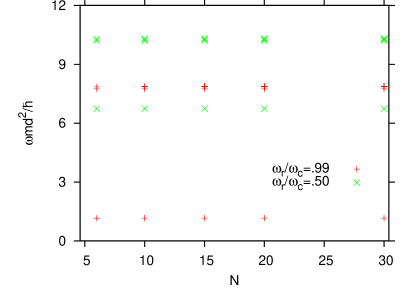
Figure 14: Normal mode frequencies (points) as a function of number of layers for two strings with a dipole strength $U=20$ and two different repulsive strengths. The modes shown here are only the intra layer modes. The cohearant full string modes behave in the same way as shown in figure 9.

The structures of the two optical modes corresponding to the degenerate energy that approaches zero are relative motions between the two molecules in each of the outermost layers. The instability is then that the amplitudes of the vibrational motion between the pairs of outer molecules become too large to return to equilibrium. The degeneracy means that all four molecules then separate simultaneously as illustrated in figure 15. Then the whole system immediately falls apart, as all shorter chains break at smaller repulsive frequencies.

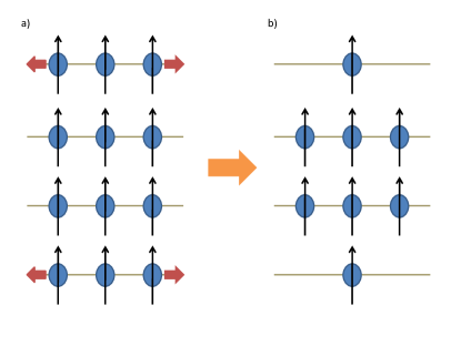
Figure 15: Schematic illustration of the unstable mode for three chains with four particles in each chain. The picture shows a 1D setup for clarity (the 2D case has a similar cylindrical structure). a) The instability of the outermost molecules in the top and bottom layers. b) The final state of the system after dissociating the two outer molcules.

If we increase the number of layers the results would be very similar. Only two differences appear. The first is that the number of repulsion-independent (horizontal) solutions increase, because the number of single chain solutions increase. The second difference is that the degeneracy increases for the highest of the optical normal modes, which involve molecules in the intermediate layers. They are essentially independent of the length of the chains, see figure 14. The lowest frequency optical mode which eventually approaches zero is also almost independent of chain length, and the unstable mode is again related to the outermost molecules.

If we instead increase the number of chains, the frequencies of the resulting solutions would appear almost precisely as in figure 13. Again only two differences appear. The first is that now the repulsive-independent (horizontal) solutions are obtained from single chain frequencies by multiplying by the square root of the number of chains. The reason is again that energies are obtained as square roots of average frequencies as explained above. The second difference is that the degeneracies increase for the two decreasing optical mode solutions. The highest of these correspond to normal modes involving molecules in the intermediate layers. They are essentially independent of the number of chains since they move pairwise without influence from the other layers. For each additional chain the degeneracy of the terminal layers increases by two, that is one corresponding to each end-layer structure. The unstable modes are now more complicated and at least one of them always involves at least one molecule of small amplitude. This implies that at least one molecule remains after the amplification of the amplitudes of the unstable mode and a subsequent breakup of the complex.

4.2 Critical stability

The structure close to the instability can be seen directly from the behaviour of $\langle(r_{i}-R)^{2}\rangle$ for the individual molecules as function of the repulsive frequency. Here $R$ is the center of mass coordinate projected on a plane. This quantity can be obtained since each molecule is treated as distinguishable. Still, identical bosons in the same layer always have the same radii. As $\omega_{r}$ increases all radii of interior molecules increase marginally whereas the terminal positions increase substantially faster. However, when $\omega_{r}$ is very close to the critical frequency, $\omega_{c}$, the internal molecule-radii perhaps double their size but the terminal sizes meanwhile increase by an order of magnitude and eventually diverge. The reflection symmetry in a central plane can be maintained throughout. Due to the circular symmetry, the system can be described as a cylinder, whose radius changes down its length, becoming wider towards the ends.

The critical frequency, $\omega_{c}$, can be found numerically by solving the Schrödinger equation. For $N$ layers and the same number of molecules in each layer, we label the molecules from $1$ to $N$ along the first chain and continue the consecutive labeling chain after chain. A formula for the critical frequency, $\omega_{c}$, and the shift, $\alpha$, can be obtained analytically by equating the repulsive and attractive potential energies as seen by one of the molecules in the outermost layer where the instability takes place

$$\frac{1}{2}\mu_{ij}\omega_{c}^{2}(x_{ij}^{2}+y_{ij}^{2})(M-1)+\frac{1}{2}\mu_{ij}\omega_{c}^{2}\alpha^{2}d^{2}(M-1)=$$

$$\frac{1}{2}\mu_{ij}(M-1)\sum_{j=2}^{N}\omega_{1j}^{2}(x_{ij}^{2}+y_{ij}^{2})+\mu_{ij}(M-1)d^{2}\sum_{j=2}^{N}\omega_{1j}^{2}(j-1)^{2}$$ , (15)

where $\omega_{1j}$ are the input frequencies reflecting the interaction between a particle in the outermost layer and layer $j$. Eliminating common factors allows one to obtain an expression for the critical frequency and the shift factor

$$\omega_{c}^{2}=\sum_{j=2}^{N}\omega_{1j}^{2},$$ (16)

and

$$\alpha^{2}=2\frac{\sum_{j=2}^{N}\omega_{1j}^{2}(j-1)^{2}}{\sum_{j=2}^{N}\omega_{1j}^{2}},$$ (17)

where the frequencies on the right hand side of equation (16) are the input frequencies determined in equation (4). These expressions hold for a system of equal masses and would have to be changed for unequal masses. The result provides the value for $\omega_{c}(N)$ which explicitly is labeled with the dependence on layers. This is a remarkably simple and very general result independent of the number of chains. The expression for $\alpha$ depends only very weakly on $U$ and $M$, and we find $\alpha^{2}\sim 2.26$ numerically for most values of $N,M,$ and $U$. The expression for $\omega_{c}$ exactly reproduces the numerically determined values. This is completely independent of $\alpha$ since, as we will discuss below, $\alpha$ is determined by equating energies of different configurations, i.e. it is a pure shift of the energy which will not influence the stability of the system. Whereas for $\alpha_{c}$ this is just a good initial guess at the proper value, which will be commented on in following sections.

Thus, $\omega_{c}(N)$ increases with number of layers, but only slowly, since smaller and smaller frequencies from more distant molecules are added to the sum in equation (16). The hierarchy of stability is now easily established, because the sequence follows the size of $\omega_{c}(N)$. If a given number of layers becomes unstable, the structure with one layer less is also unstable. On the other hand, we find that the critical repulsion is independent of the number of chains.

So far we considered systems with the same number of molecules in all layers. The normal modes are then related to symmetric structures essentially localized as motion within planes and relative motion between groups of molecules in different planes. A different system could have fewer molecules in the outer layers than the series of identical layers in the interior, an example is shown in figure 15b). The hierarchy of stability follows from the number of repulsions in the outer layers, that means one molecule is most stable, two second most, etc.

The critical frequency for a configuration with one molecule in the outer layers, $\tilde{\omega}_{c}$, is found to be

$${\tilde{\omega}}_{c}^{2}=\omega_{c}^{2}(N-2)+\frac{1}{M}(\omega_{12}^{2}+\omega_{2N}^{2})\;,$$ (18)

where we used the definition in equation (16), the labeling are that molecules $1$ and $N$ are the lone outer molecules, and molecule $2$ is in the second layer with $M$ molecules. Interestingly, the ratio, ${\tilde{\omega}}_{c}^{2}/\omega_{c}^{2}(N)$, seems to be independent of the dipole strength.

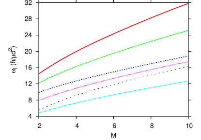
Figure 16: Single chain modes as a function of number of chains, $M$, for a broken system of 6 layers (where now there is only one molecule in the outermost layers). The lines connect the same normal mode at a given number of chains. The dashed black line is the frequency of the degenerate mode which is not the breaking mode frequency taken when $\omega_{r}\approx\omega_{c}$. The dipole strength was $U=20$.

The behaviour of the normal modes and normal mode frequencies is similar to the complete system. The total number of remaining modes is $M(N-2)+1$. The $N-1$ single chain modes remain, and they appear qualitatively just as seen in figure 12. These frequencies increase with the number of chains, and are shown in figure 16, but no longer in the square root dependence that was seen in the complete system. As with the unbroken system, the single chain frequencies do not change with the repulsive frequency. The remaining modes fall into two degenerate groups of equal size, $2(M-1)$. One group approaches zero as the repulsive frequency is increased, while the remaining modes are at a frequency between the two lowest single chain modes. The group approaching zero are modes involving the outermost full layers, which become unstable as the frequency is increased. The other group are modes in the central layers.

Another question is which structure the unstable mode has when only one molecule occupies the outer layers. The unstable mode is moved to the next-to-outermost layers where the molecules close to the critical frequency then behave as in the system where they were in the outer layers. The resulting configuration is then most likely one molecule in each of the two outer layers in each end. This configuration is stable because the decrease of $\omega_{c}^{2}(N-2)$ to the value $\omega_{c}^{2}(N-4)$ is compensated by the added dominating term, $\omega_{12}^{2}$, as seen in equation (18). Increasing the repulsion would repeat the process of instability of the next fully occupied layers. The system seems to prefer to approach single chain structure.

If we decrease the number of molecules in the outer layers by one molecule at a time, the instability is seen as degenerate modes of varying frequency approaching zero for sufficiently strong repulsion. The degeneracy corresponds to an instability in the outer layer until the outer layer has just more than half as many molecules as the second layer. Then the degeneracy changes to correspond to instability of the molecules in the second layer. This reflects that the instabilty is initially related to the outer layer until a number of molecules is removed from that layer and the second layer contains the unstable mode. Regarding the critical frequencies, for the outermost layer, the critical frequency is

$${\tilde{\omega}}_{c}^{2}=\omega_{c}^{2}(N-2)+\omega_{1N}^{2}+\omega_{2N}^{2}+\frac{h}{M-h}\sum_{k=2}^{N-1}\omega_{1k}^{2},$$ (19)

where $h$ is the number of holes in the outermost layer, and $\omega_{1j}$ is the interaction frequency between layer one and layer $j$. For the molecules in the penultimate layer, the critical frequency is

$${\tilde{\omega}}_{c}^{2}=\omega_{c}^{2}(N-2)+\frac{M-h}{M}(\omega_{12}^{2}+\omega_{2N}^{2}).$$ (20)

Whichever of these two frequencies is lower for a given configuration determines in which layer the instability lies.

In summary, for the frequencies, there are a total of $NM-1$ normal mode frequencies. A subset, $N-1$ of them, are single string modes with frequency equal to $\sqrt{M}$ the frequency of the corresponding single string mode. There are then many degenerate modes, $2(M-1)$ of them go to zero as the repulsive frequency is increased. This is because the chain breaks by removing the repulsion in the outermost layers, releasing all but one molecules. The remaining degenerate frequencies cluster into groups, and are often very close to each other in magnitude. They also decrease as the repulsive frequency is increased, similar to what is seen in figure 13 for two strings.

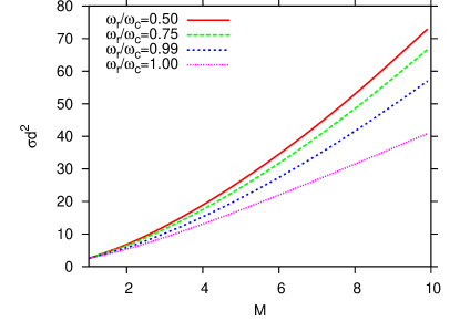
Figure 17: Density of the central molecules as a function of number of chains. Each chain is eight molecules long and the dipole strength was $U=20$.

5 Density and energy relations

The repulsive frequency and the repulsive shift are so far left as free parameters, although we did discuss at length how one can relate them to two-body properties in section 2. The shift is only related to total energies without any influence on structures. We need to define a zero point to measure from but this requires more than two molecules, and the criterion easily depends on which system was used for the calibration. In the next subsections we deal with these two parameters in the in-layer repulsion.

5.1 Density versus repulsive frequency

In a system with many layers, the density depends on the relative position of the layer. To be specific we consider the central layers where the density is rather constant across a few layers. The outer layers close to the critical stability are on the other hand expanding as the breaking point is approached. Already for a relatively small number of layers this expansion only affects the outer layers. We thus define the density through the average radii of the central layers, i.e.

$$\rho=\frac{M}{\pi\langle\bar{r}^{2}\rangle}\;,\;\;\;\langle\bar{r}^{2}\rangle=\frac{1}{M}\sum_{k=1}^{M}\langle(r_{k}-R)^{2}\rangle\;,$$ (21)

where this definition is valid for non-identical molecules. The densities of the central layers defined in equation (21) are seen in figure 17 for different repulsions as functions of number of molecules in each layer. These curves are essentially independent of chain length, but increase with molecule number and decreasing repulsion.

The density of the central layers are essentially independent of chain length. It does depend, however, on the dipole strength, molecules per layer, $M$, and the repulsive frequency, i.e., $\rho\propto\sigma(M,\omega_{r},U)$ with a very weak dependence on $N$. The dependence on $M$ is a straightforward $M^{3/2}$, which comes from, in eq (21), with one power of $M$ in the numerator, and it is found that $\langle r_{k}^{2}\rangle$ goes like $M^{-1/2}$. The critical frequency, and hence the critical density, below which the system becomes unstable, depends on the parameters as mentioned above. We can state explicitly the dependence on $M$, and thus try to isolate its dependence on frequency, and thus $U$:

$$\rho_{c}\propto M^{3/2}\omega_{c}(N,U),$$ (22)

though the dependence on $N$ is very weak. The dependence on $\omega_{c}$ is linear, and the dependence of $\omega_{c}(N,U)$ on $U$ is seen in figure 18. One can see that the dependence on the length of the chain, $N$, is indeed very weak. However, in looking at densities of central layers, one must have a chain of 4-5 layers in order for a ”central layer” to be clearly defined. A plot of the density as a function of intermediate values of the repulsion is seen in figure 19. One can see that when the chain lengths are doubled, the curves are almost indistinguishable. The relations between the lines that differ in the other parameters are as described in eq (22). The behaviour of the curve is not analytical, but the ratio $\rho(\omega_{r}=0)/\rho_{c}\doteq 1.39$, where $\rho(\omega_{r}=0)$ is the density with zero repulsion, is seen for all the sets of parameters.

In section 2, we discussed the option of relating the magnitude of the repulsive frequency to density (see (8)), but did, however, caution that this is not a very desirable approach to effective interactions in the $N$-body problem. The density that we obtain within our model can become very large. In fact, if we insert the obtained densities of order $\sigma d^{2}\sim 10-100$ in (8), the frequency obtained is larger than the critical frequency by an order of magnitude already for $M=3$ and increases rapidly with $M$. This shows the dominance of the attractive interlayer forces, i.e. the system contracts into denser configuration than the typical average experimental density. We stress again that (8) is a questionable relation but note that the alternative way of fixing the repulsion through the bound state structure of the potentials also predicts a repulsion slightly beyond the critical value. So in a system where the inter- and intralayer dipolar strength is the same, we expect the configurations with multiple molecules in single layer to be unstable.

An important point here is that the critical frequency is essentially independent of $M$, i.e., if we add another chain to the system for a fixed value of $\omega_{r}<\omega_{c}(N,U)$. On the other hand, the density goes up since the additional attractive interlayer terms that balance the extra repulsion in each layer will make the system contract. According to (8) this implies that $\omega_{r}$ should be increased and it will then quickly exceed $\omega_{c}(N,U)$. Again, it is unfortunate to change the two-body interactions in response to a property of the total system. By allowing the repulsion to be a free parameter we can study the detailed competition between repulsive and attractive term in the system which was one goal of the current study.

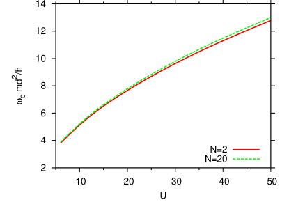
Figure 18: Critical frequency for two chains of differing lengths as a function of interaction strength.

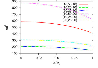
Figure 19: Densities as a function of the ratio of the repulsive frequency to the critical repulsive frequency. This is plotted for several values of the parameters $N,M,$ and $U$, and the curves are identified by the label $(N,M,U)$.

5.2 Energy versus repulsive shift

The relative energies depend on the repulsive shift in equation (7). A consistent choice of scale factor, $\alpha$, independent of chain $M$, and layer, $N$, numbers is not possible. The problems arise, because instability towards some continuum structure is found through the lack of solutions, and totally independent of the energy of the configurations. However, the repulsive shift is precisely able to adjust energies such that the wave function and energy criterion coincide for specific geometries. The main effects can be included by an appropriate choice.

The constant, $\alpha$, may be obtained by comparing the energies of one system at the point of instability with the other system formed after breaking apart. The constant is adjusted so that the energies of these systems are the same at the breaking frequency. Let us choose the simplest structure with three molecules in each layer and compare to the system where two molecules are removed from each of the end-layers. This requirement leads to $\alpha\sim 1.92$, which makes the repulsive shift somewhat weak compared to the attractive one at the breaking frequency. This choice of $\alpha$ has the nice feature that as the number of molecules per layer is increased, the energy becomes more negative, but does not run away to negative infinity. This is a nice feature since we know that the breaking frequency is independent of $M$. However, this value of $\alpha$ will not match energies when the system is driven to its breaking frequency. A better form for the constant might be

$$\alpha^{2}=\alpha_{0}^{2}\pm\alpha_{1}^{2}/M,$$ (23)

where $\alpha_{0}$ is obtained by fitting to the quadratic dependence of the energies of $M$ in systems where $M\geq~{}5$. The second constant, $\alpha_{1},$ is determined by matching the energies of a complete system, and the system where one molecule has been removed from both of the outermost layers (where it is assumed that the $\alpha_{0}$ term will cancel). This combines two desirable features, controlling the energy dependence on $M$ and matching with the broken system. These constants were determined for the system $(N,M)=(6,8)$ and $U=20$ to be $(\alpha_{0},\alpha_{1})=(1.9761,3.0123)$, and the lower sign is taken in equation (23). These constant do what is prescribed of them, but do have drawbacks. For example, for $M=2$, the overall sign is negative, which makes it an additional attractive shift. Also, while the energies at breaking match at $M=8$, at $M=9$ they already are mismatched by 1.2%. Clearly one value of $\alpha$ cannot accurately reproduce all the desired properties of the total energies. A reasonable average choice is $\alpha\sim 1.92$ but more accuracy can be achieved by focussing locally on a specific system and tune the value of $\alpha$.

This value of $\alpha\sim 1.92$ was cited in the discussion of the two-body repulsive interactions in section 2 and leads to a reasonably low $\omega_{r}$, which is, however, still larger than the critical frequency for breakup. Again we remark that $\alpha$ is a geometric quantity related to the form of the inverted oscillator that provides the repulsion.

By increasing the number of chains, or increasing the number of molecules in each layer of the cylinder, we are essentially adding another dimension to the system, a number of molecules per layer in addition to the length of the chains. For a system of $M$ chains of $N$ molecules, one can count the number of attractive and repulsive pairs in the system. If we keep to the nearest neighbour level of attraction, then the number of attractive pairs is $M^{2}(N-1)$, and the number of repulsive terms is $M(M-1)N/2$. Their ratio is then

$$\textrm{Attractive pairs}/\textrm{Repulsive pairs}=\frac{2M(N-1)}{N(M-1)}.$$ (24)

This ratio appears, for example, in the bilayer system ($N=2$), where if one keeps adding more pairs of molecules (one in each layer per pair), the ratio of attraction to repulsion decreases from two ($M=2$) to one ($M\gg 1$). One might expect that this would influence the critical repulsive frequency, but this frequency does not change with the addition of more chains. In the nearest neighbour approximation, it would also not change with increasing the chain length. It is the interaction beyond the nearest neighbour that can affect the critical frequency. The relation can, however, affect the energetics of the system, depending on the relative strengths of the attraction and repulsion. As mentioned before, this indicates that a scale factor defined for a system with only three chains $(M=3)$, would be too large if used for systems with large $M$, as the ratio of attractions to repulsions falls as $M$ increases (for fixed $N$).

An example application of the scale factor is for a system of ten chains of six molecules, where molecules are removed as the repulsion is increased. The molecules are removed from the layer indicated by the degeneracy of the normal mode frequency that is going to zero at the critical repulsive frequency. It was found that the energetics correctly describe the order of the removal, which can be seen in figure 20. When plotted relative to the ground state energy (and scaled down because the energies are quite large in our units), the point where the degeneracies switched to the penultimate layer was also energetically lower than continuing to remove molecules from the outermost layer. For the figure, the constants in the repulsive shift were those quoted above for the system of $(N,M)=(6,8)$, so one can see the mismatch for the removed molecules already appearing, as there should be no energy difference between the full system and the system where one molecule has been removed from the outermost layer at the critical frequency. Thus if one is interested in detailed energetics, one should decide on a shift energy in the region where one is interested in doing calculations.

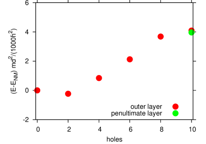
Figure 20: Energies relative to the full six layers of ten molecule system, i.e., $(N,M)=(6,10)$ as molecules are removed from the outermost layers. molecules are removed one-by-one from both outer layers, in order to preserve the symmetry about the center layer of the system. When performing the calculation in a system where molecules have been removed, the repulsive frequency used is the critical frequency of the parent system. This was not done for the the system where ten molecules where removed, since the $\omega_{c}$(8 holes)$>\omega_{c}$(10 holes). For this system with ten holes, the calculations were done for the two different geometries: five holes in each outer layer, and with four holes in the outer layer and one in the penultimate layer, at the critical frequency of the latter geometry, which is the lower of the two and lower than that of the parent system.

6 Summary and Conclusion

We have discussed how the harmonic approximation can be used to study the $N$-body 2D problem of dipole-dipole interacting molecules. First the two-body interaction is approximated by a shifted harmonic oscillator potential with the same negative and positive spatial regions. The frequency is then determined as function of the molecular dipole moment by the requirement that the two-body energy has to be reproduced. We test this procedure by comparing with the exact energy of three and four molecules in separate layers. The approximation is remarkably accurate over the range of available dipole moments. The repulsion between in-layer molecules is also approximated by a shifted harmonic oscillator but now we leave the frequency as a parameter which can be related to properties of larger bound state structures when they become available from exact calculations.

The basic ingredient is a chain where one molecule is placed in each layer where the intralayer repulsion then is absent. We calculate the binding energy in units of the two-body energy of the number of neighbouring pairs, and find a weak increase as function of molecule number. The value is always only slightly larger than the analytical estimate of $\zeta(3)$ which is approached for large dipole moment. Weaker interactions result in about $10\%$ larger values reflecting more correlation along the chain. The nearest neighbours contribute by more than $80\%$ of the energy. The spatial extension in the planes measured in units of the layer distance from the total center of mass position increases from central towards the outer layer. The weaker the interaction the larger is the size. The normal modes are oscillations away from equilibrium with a different number of nodes. All frequencies of the normal modes increase with interaction strength, while the lowest of these always decrease with increasing molecule number.

The normal modes of the single chain configuration are equivalent to those obtained in the theory of acoustic phonons in crystals. By fitting our numerical results for the lowest mode frequencies, one can obtain the speed of sound in the chain. We found that the speed of sound was more than a factor of three less than what one would naively get by expanding the dipole potential around the origin to quadratic order. This reflects one of the differences of our procedure for obtaining an effective harmonic approximation through the exact two-body bound state energy and the potential profile. The latter approach gives an effective more shallow potential which results in a smaller string tension and a reduced speed of sound. This indicates a short-coming of the naive harmonic approach in describing the collective behaviour of a chain of dipoles.

We proceed to investigate two chains consisting of two molecules in each layer. The structure of the system is most clearly found through its excitation modes, or specifically the normal modes. The repulsive intralayer interaction is varied from zero to the critical value where the system becomes unstable as seen by a vanishing normal mode frequency. The normal modes fall into two distinct groups. The first group is independent of the intralayer repulsion with a simple one-to-one correspondence to the one-chain modes. These modes correspond to in-phase motion of the two chains. The energies of the second group decrease with repulsion and the lowest of these modes vanishes at the critical value. These modes correspond to in-layer oscillations breaking the one-chain structure. This is analagous to optical modes in crystals with more than one atoms at each lattice site. The breakup is seen through diverging amplitudes on the molecules in the two outer layers.

Increasing the number of chains so that there are more molecules in each layer leads to remarkably similar behaviour of the normal mode frequencies. The one-to-one correspondence with one-chain modes remains. Furthermore, the decreasing normal mode frequencies also vanish at the same critical repulsion which then is independent of the the number of molecules in the layers. However, the degeneracy increases in correspondence to the increase in the number of degrees of freedom within one layer. This implies that the configuration at the breaking point has diverging amplitudes of the molecules in the two outer layers. The breaking then leads to a system where the two outer layers have fewer molecules than the more central layers. These configurations have less repulsion and the next instability is related to removal of molecules from the next two outer layers. This peeling off molecules would continue to the third outermost layer or remove more molecules in the outer layers. Eventually one chain only would remain. We also calculate the density of the central layers and find that it is independent of the number of layers, depending on the number of molecules per layer to the power $3/2$ with a factor that depends on the dipolar strength.

The structures are independent of the constant shifts in the repulsive potential terms which only have influence on the relative energies. We choose these shifts such that the energy of the system at the critical frequency is the same as the most likely combination of fragments. We adjust to relatively large numbers of layers and molecules in each layer. Then we compare energies of a system and two systems of half the sizes either in layers or molecules in the layers. We conclude that the more layers, the more stable is the system, whereas the energy is rather independent of the number of molecules in each layer.

In conclusion, the harmonic approximation is very useful in the description of the two-dimensional systems of cold polar molecules. However, this requires a careful adjustment of the forces between molecules in different planes and in the same plane. The latter can be particularly tricky to define and we have discussed at length how to describe the in-plane repulsion in a reasonable way using an inverted harmonic oscillator potential. Using a harmonic approximation for both types of interaction is very desirable due to its exact solvability. The structures are found as function of layers and molecules in the layers, energies and sizes are calculated, and configurations of excitation modes are found. The structures are ordered in a hierarchy related to their stability.

The results obtained here within the harmonic model indicate that for a typical system where the strength of the inter-layer and intra-layer terms are both proportional to the square of the dipole moment, bound complexes with more than one molecules in a single layer are not bound and that the single chains with one molecule in each layer are the stable entities. However, the external confinement that any realistic experiment employs means that the dipoles cannot separate to large distances. We therefore expect that the multi-chain modes calculated in the harmonic model could show up as resonances. Here we provide a study of these modes and the breakup channels of multi-chain complexes.

The experimental conditions needed to study the systems considered here should be within reach of the next generation of cold polar molecular experiments. The current front-runner uses ⁴⁰K⁸⁷Rb molecules which have $U=0.1$ for the condition in Ref. miranda2011 , but which can probably be extended up to about $U=1.2$ with increasing electric field. These values of $U$ are likely too small for the harmonic approximation used here to apply since the two-body bound states are very extended armstrong2010 . However, most other combinations of alkali atoms into polar molecules can potentially be used at dipole moments of 1 Debye or more julienne2011 , which would easily increase $U$ by one or two orders of magnitude. Larger values of $U$ implies that the single chain structures will have large binding energies, and in turn be stable even in thermal samples. This means that one does not necessarily need to be in the nano-Kelvin temperature regime to study the chains discussed in the current work.

The current work indicates that the structure of a multi-layer system with several particles in each layer is most likely that of single chains, i.e. the dipolar chains liquid originally proposed in Ref. wang2006 , but that more complex states are possible if the intralayer repulsion could be somehow tuned independently of the interlayer attraction. This could perhaps be obtained by using a combination of external electric fields and applied lasers giovanazzi2002 ; micheli2007 ; gorshkov2008 .

References

- (1) S. Ospelkaus et al., Nature Phys. 4, 622 (2008);
- (2) K.-K. Ni et al., Science 322, 231 (2008);
- (3) J. Deiglmayr et al., Phys. Rev. Lett. 101, 133004 (2008);
- (4) F. Lang et al., Phys. Rev. Lett. 101, 133005 (2008);
- (5) D. Wang et al., Phys. Rev. A 81, 061404(R) (2010);
- (6) B. C. Sawyer et al., Phys. Chem. Chem. Phys. 13, 19059 (2011)
- (7) K-.K. Ni et al., Nature 464 1324, (2010)
- (8) S. Ospelkaus et al., Science 327 853, (2010)
- (9) L. D. Carr, D. DeMille, R. V. Krems, and J. Ye, New J. Phys. 11, 055049 (2009)
- (10) M. G. H. de Miranda et al., Nature Phys. 7, 502 (2011)
- (11) M. A. Baranov, Phys. Rep. 464, 71 (2008);
- (12) T. Lahaye, C. Menotti, L. Santos, M. Lewenstein, and T. Pfau, Rep. Prog. Phys. 72, 126401 (2009)
- (13) K. Góral, L. Santos, and M. Lewenstein, Phys. Rev. Lett. 88, 170406 (2002);
- (14) D. DeMille, Phys. Rev. Lett. 88, 069701 (2002);
- (15) R. Barnett, D. Petrov, M. Lukin, and E. Demler, Phys. Rev. Lett. 96, 190401 (2006);
- (16) A. Micheli, G. K. Brennen, and P. Zoller, Nature Phys. 2, 341 (2006).
- (17) D.-W. Wang, M. D. Lukin, and E. Demler, Phys. Rev. Lett. 97, 180413 (2006)
- (18) P. M. Lushnikov, Phys. Rev. A 66, 051601 (2002)
- (19) A. Micheli, Z. Idziaszek, G. Pupillo, M. A. Baranov, P. Zoller, and P. S. Julienne, Phys. Rev. Lett. 105, 073202 (2010)
- (20) S.-M. Shih and D.-W. Wang, Phys. Rev. A 79, 065603 (2009);
- (21) D. V. Fedorov, J. R. Armstrong, N. T. Zinner, and A. S. Jensen, Few-body Syst. 50, 417 (2011);
- (22) M. Klawunn, A. Pikovski, and L. Santos, Phys. Rev. A 82, 044701 (2010);
- (23) B. Wunsch, N. T. Zinner, I. B. Mekhov, S.J. Huang, D.-W. Wang, and E. Demler, Phys. Rev. Lett. 107, 073201 (2011)
- (24) N. T. Zinner, B. Wunsch, I. B. Mekhov, S.J. Huang, D.-W. Wang, and E. Demler, Phys. Rev. A 84, 063606 (2011)
- (25) A. G. Volosniev, D. V. Fedorov, A. S. Jensen, and N. T. Zinner, Phys. Rev. A 85, 023609 (2012)
- (26) J. C. Cremon, G. M. Bruun, and S. M. Reimann, Phys. Rev. Lett. 105, 255301 (2010)
- (27) J. R. Armstrong, N. T. Zinner, D. V. Fedorov, and A. S. Jensen, Europhys. Lett. 91 16001 (2010)
- (28) A. G. Volosniev, D. V. Fedorov, A. S. Jensen, and N. T. Zinner, Phys. Rev. Lett. 106, 250401 (2011);
- (29) A. G. Volosniev, N. T. Zinner, D. V. Fedorov, A. S. Jensen, and B. Wunsch, J. Phys. B 44, 125301 (2011)
-
(30)
N. T. Zinner, J. R. Armstrong, A. G. Volosniev, D. V. Fedorov, and A. S. Jensen,
Few-Body Syst. Online First (2012), eprint
arXiv:1105.6264v2 - (31) G. M. Bruun and E. Taylor, Phys. Rev. Lett. 101, 245301 (2008);
- (32) R. M. Lutchyn, E. Rossi, and S. Das Sarma, Phys. Rev. A 82, 061604(R) (2009);
- (33) N. R. Cooper and G. V. Shlyapnikov, Phys. Rev. Lett. 103, 155302 (2009);
- (34) K. Sun, C. Wu, and S. Das Sarma, Phys. Rev. B 82, 075105 (2010);
- (35) Y. Yamaguchi, T. Sogo, T. Ito, and T. Miyakawa, Phys. Rev. A 82, 013643 (2010);
- (36) A. Pikovski, M. Klawunn, G. V. Shlyapnikov, and L. Santos, Phys. Rev. Lett. 105, 215302 (2010);
- (37) F. Herrera, M. Litinskaya, R. V. Krems, Phys. Rev. A 82, 033428 (2010);
- (38) L. Pollet, J. D. Picon, H. P. Büchler, and M. Troyer, Phys. Rev. Lett. 104 125302 (2010);
- (39) N. T. Zinner, B. Wunsch, D. Pekker, and D.-W. Wang, Phys. Rev. A 85, 013603 (2012);
- (40) N. T. Zinner and G. M. Bruun G M, Eur. Phys. Jour. D 65, 133 (2011);
- (41) J. Levinsen, N. R. Cooper, and G. V. Shlyapnikov, Phys. Rev. A 84, 013603 (2011);
- (42) L. He, W. Hofstetter, Phys. Rev. A 83, 053629 (2011)
- (43) E. Wigner, Phys. Rev. 46, 1002 (1934);
- (44) L. Bonsall and A. A. Maradudin, Phys. Rev. B 15, 1959 (1977)
- (45) R. K. Kalia and P. Vashishta, J. Phys. C 14, L643 (1981);
- (46) V. M. Bedanov, G. V. Gadiyak, Yu. E. Lozovik, JETP 61, 967 (1985)
- (47) C. Mora, O. Parcollet, and X. Waintal, Phys. Rev. B 76, 064511 (2007);
- (48) H. P. Büchler et al., Phys. Rev. Lett. 98, 060404 (2007);
- (49) G. E. Astrakharchik, J. Boronat, I. L. Kurbakov, and Yu. E. Lozovik, Phys. Rev. Lett. 98, 060405 (2007)
- (50) A. S. Arkhipov, G. E. Astrakharchik, A. V. Belikov, and Yu E. Lozovik, JETP Lett. 82, 39 (2005);
- (51) P. Rabl and P. Zoller, Phys. Rev. A 76, 042308 (2007);
- (52) C. Menotti, C. Trefzger, and M. Lewenstein, Phys. Rev. Lett. 98, 235301 (2007);
- (53) C. Kollath, J. S. Meyer, and T. Giamarchi, Phys. Rev. Lett. 100, 130403 (2008);
- (54) R. Citro, E. Orignac, S. De Palo, and M. L. Chiofalo, Phys. Rev. A 75, 051602 (2007);
- (55) G. E. Astrakharchik, G. Morigi, G. De Chiara, and J. Boronat, Phys. Rev. A 78, 063622 (2008);
- (56) Y.-P. Huang and D.-W. Wang, Phys. Rev. A 80, 053610 (2009);
- (57) C.-M. Chang, W.-C. Shen, C.-Y. Lai, P. Chen, and D.-W. Wang, Phys. Rev. A 79, 053630 (2009)
- (58) S. Fishman, G. De Chiara, T. Calarco, and G. Morigi, Phys. Rev. B 77, 064111 (2008);
- (59) P. F. Herskind, A. Dantan, J. Marler, M. Albert, and, M. Drewsen, Nature Phys. 5, 494 (2009)
- (60) J. Quintanilla, S. T. Carr, and J. J. Betouras, Phys. Rev. A 79, 031601(R) (2009);
- (61) S. T. Carr, J. Quintanilla, and J. J. Betouras, Phys. Rev. B 82, 045110 (2010)
- (62) K.-Y. Zhu, L. Tan, X. Gao, and D.-W. Wang, Chin. Phys. Lett. 25, 48 (2008)
- (63) M. Klawunn, J. Duhme, and L. Santos, Phys. Rev. A 81, 013604 (2010)
- (64) X. Lu, C.-Q. Wu, A. Micheli, and G. Pupillo, Phys. Rev. B 78, 024108 (2008)
- (65) B. Capogrosso-Sansone and A. Kuklov, Jour. Low Temp. Phys. 165, 213 (2011)
- (66) J. R. Armstrong, N. T. Zinner, D. V. Fedorov, and A. S. Jensen, J. Phys. B 44, 055303 (2011)
- (67) N. N. Khuri, A. Martin, and T.-T. Wu, Few-body Syst. 31, 83 (2002)
- (68) S. Giovanazzi, A. Gørlitz, and T. Pfau, Phys. Rev. Lett. 89, 130401 (2002)
- (69) A. Micheli, G. Pupillo, H. P. Büchler, and P. Zoller, Phys. Rev. A 76, 043604 (2007)
- (70) A. V. Gorshkov, P. Rabl, G. Pupillo, A. Micheli, P. Zoller, M. D. Lukin, and H. P. Büchler, Phys. Rev. Lett. 101, 073201 (2008)
- (71) A. S. Jensen, K. Riisager, D. V. Fedorov, and E. Garrido, Rev. Mod. Phys. 76, 215 (2004).
- (72) G. E. Astrakharchik, G. B. De Chiara, G. Morigi, and J. Boronat, J. Phys. B. 42, 154026 (2009)
- (73) P. S. Julienne, T. M. Hanna, Z. Idziaszek, Phys. Chem. Chem. Phys. 13, 19114 (2011)