Asymptotic optimality of the Westfall–Young permutation procedure for multiple testing under dependence

Abstract

Test statistics are often strongly dependent in large-scale multiple testing applications. Most corrections for multiplicity are unduly conservative for correlated test statistics, resulting in a loss of power to detect true positives. We show that the Westfall–Young permutation method has asymptotically optimal power for a broad class of testing problems with a block-dependence and sparsity structure among the tests, when the number of tests tends to infinity.

T1N. Meinshausen and M. H. Maathuis contributed equally to this work.

,
and

1 Introduction

We consider multiple hypothesis testing where the underlying tests are dependent. Such testing problems arise in many applications, in particular, in the fields of genomics and genome-wide association studies hirschhorn2005genome , mccarthy2008genome , dudoit2008multiple , but also in astronomy and other fields liang02statistical , meinshausen04estimating . Popular multiple-testing procedures include the Bonferroni–Holm method holm79simple which strongly controls the family-wise error rate (FWER), and the Benjamini–Yekutieli procedure benjamini01control which controls the false discovery rate (FDR), both under arbitrary dependence structures between test statistics. If test statistics are strongly dependent, these procedures have low power to detect true positives. The reasons for this loss of power are well known: loosely speaking, many strongly dependent test-statistics carry only the information equivalent to fewer “effective” tests. Hence, instead of correcting among many multiple tests, one would in principle only need to correct for the smaller number of “effective” tests. Moreover, when controlling some error measure of false positives, an oracle would only need to adjust among the tests corresponding to true negatives. In large-scale sparse multiple testing situations, this latter issue is usually less important since the number of true positives is typically small, and the number of true negatives is close to the overall number of tests.

The dependence among tests can be taken into account by using the permutation-based Westfall–Young method westfall93resampling , already used widely in practice (e.g., cheung2005mapping , winkelmann2007genome ). Under the assumption of subset-pivotality (see Section 2.3 for a definition), this method strongly controls the FWER under any kind of dependence structure WestfallYoung89 .

In this paper we show that the Westfall–Young permutation method is an optimal procedure in the following sense. We introduce a single-step oracle multiple testing procedure, by defining a single threshold such that all hypotheses with $p$-values below this threshold are rejected (see Section 2.2). The oracle threshold is the largest threshold that still guarantees the desired level of the testing procedure. The oracle threshold is unknown in practice if the dependence among test statistics and the set of true null hypotheses are unknown. We show that the single-step Westfall–Young threshold approximates the oracle threshold for a broad class of testing problems with a block-dependence and sparsity structure among the tests, when the number of tests tends to infinity. Our notion of asymptotic optimality relative to an oracle threshold is on a general level and for any specified test statistic. The power of a multiple testing procedure depends also on the data generating distribution and the chosen individual test(s): we do not discuss this aspect here. Instead, our goal is to analyze optimality once the individual tests have been specified.

Our optimality result has an immediate consequence for large-scale multiple testing: it is not possible to improve on the power of the Westfall–Young permutation method while still controlling the FWER when considering single-step multiple testing procedures for a large number of tests and assuming only a block-dependence and sparsity structure among the tests (and no additional modeling assumptions about the dependence or clustering/grouping). Hence, in such situations, there is no need to consider ad-hoc proposals that are sometimes used in practice, at least when taking the viewpoint that multiple testing adjusted $p$-values should be as model free as possible.

1.1 Related work

There is a small but growing literature on optimality in multiple testing under dependence. Sun and Cai sun2009large studied and proposed optimal decision procedures in a two-state hidden Markov model, while Genovese et al. genovese2006false and Roeder and Wasserman roeder2009genome looked at the intriguing possibility of incorporating prior information by $p$-value weighting. The effect of correlation between test statistics on the level of FDR control was studied in Benjamini and Yekutieli benjamini01control and Benjamini et al. benjamini2006adaptive ; see also Blanchard and Roquain blanchard2009adaptive for FDR control under dependence. Furthermore, Clarke and Hall clarke2009robustness discuss the effect of dependence and clustering when using “wrong” methods based on independence assumptions for controlling the (generalized) FWER and FDR. The effect of dependence on the power of Higher Criticism was examined in Hall and Jin hall2008properties , hall2010innovated . Another viewpoint is given by Efron efron2007correlation , who proposed a novel empirical choice of an appropriate null distribution for large-scale significance testing. We do not propose new methodology in this manuscript but study instead the asymptotic optimality of the widely used Westfall–Young permutation method westfall93resampling for dependent test statistics.

2 Single-step oracle procedure and the Westfall–Young method

After introducing some notation, we define our notion of a single-step oracle threshold and describe the Westfall–Young permutation method.

2.1 Preliminaries and notation

Let $W$ be a data matrix containing $n$ independent realizations of an $m$-dimensional random variable $X=(X_{1},\ldots,\allowbreak X_{m})$ with distribution $P_{m}$ and possibly some additional deterministic response variables $y$.

Prototype of data matrix $W$. To make this more concrete, consider the following setting that fits the examples described in Section 3.2. Let $y$ be a deterministic variable, and allow the distribution of $X=X_{y}$ to depend on $y$. For each value $y^{(i)}$, $i=1,\ldots,n$, we observe an independent sample $X^{(i)}=(X^{(i)}_{1},\ldots,X^{(i)}_{m})$ of $X=X_{y^{(i)}}$. We then define $W$ to be an $(m+1)\times n$-dimensional matrix by setting $W_{1,i}=y^{(i)}$ for $i=1,\ldots,n$ and $W_{j+1,i}=X_{j}^{(i)}$ for $j=1,\ldots,m$ and $i=1,\ldots,n$. Thus, the first row of $W$ contains the $y$-variables, and the $i$th column of $W$ corresponds to the $i$th data sample $(y^{(i)},X^{(i)})$.

Based on $W$, we want to test $m$ null hypotheses $H_{j}$, $j=1,\ldots,m$, concerning the $m$ components $X_{1},\ldots,X_{m}$ of $X$. For concrete examples, see Section 3.2. Let $I(P_{m})\subseteq\{1,\ldots,m\}$ be the indices of the true null hypotheses, and let $I^{\prime}(P_{m})$ be the indices of the true alternative hypotheses, that is, $I^{\prime}(P_{m})=\{1,\ldots,m\}\setminus I(P_{m})$. Let $P_{0}$ be a distribution under the complete null hypothesis, that is, $I(P_{0})=\{1,\ldots,m\}$. We denote the class of all distributions under the complete null hypothesis by $\mathcal{P}_{0}$.

Suppose that the same test is applied for all hypotheses, and let $S_{n}\subseteq[0,1]$ be the set of possible $p$-values this test can take. Thus, $S_{n}=[0,1]$ for $t$-tests and related approaches, while $S_{n}$ is discrete for permutation tests and rank-based tests. Let $p_{j}(W)$, $j=1,\ldots,m$, be the $p$-values for the $m$ hypotheses, based on the chosen test and the data $W$.

2.2 Single-step oracle multiple testing procedure

Suppose that we knew the true set of null hypotheses $I(P_{m})$ and the distribution of $\min_{j\in I(P_{m})}p_{j}(W)$ under $P_{m}$ (which is of course not true in practice). Then we could define the following single-step oracle multiple testing procedure: reject $H_{j}$ if $p_{j}(W)\leq c_{m,n}(\alpha)$, where $c_{m,n}(\alpha)$ is the $\alpha$-quantile of $\min_{j\in I(P_{m})}p_{j}(W)$ under $P_{m}$.

$$c_{m,n}(\alpha)=\max\Bigl{\{}s\in S_{n}\dvtx P_{m}\Bigl{(}\min_{j\in I(P_{m})}p_{j}(W)\leq s\Bigr{)}\leq\alpha\Bigr{\}}.$$ (1)

Throughout, we define the maximum of the empty set to be zero, corresponding to a threshold $c_{m,n}(\alpha)$ that leads to zero rejections.

This oracle procedure controls the FWER at level $\alpha$, since, by definition,

$$P_{m}\bigl{(}H_{j}\mbox{ is rejected for at least one }j\in I(P_{m})\bigr{)}$$

$$\qquad=P_{m}\Bigl{(}\min_{j\in I(P_{m})}p_{j}(W)\leq c_{m,n}(\alpha)\Bigr{)}\leq\alpha,$$

and it is optimal in the sense that values $c\in S_{n}$ with $c>c_{m,n}(\alpha)$ no longer control the FWER at level $\alpha$.

2.3 Single-step Westfall–Young multiple testing procedure

The Westfall–Young permutation method is based on the idea that under the complete null hypothesis, the distribution of $W$ is invariant under a certain group of transformations $\mathcal{G}$, that is, for every $g\in\mathcal{G}$, $gW$ and $W$ have the same distribution under $P_{0}\in\mathcal{P}_{0}$. Romano and Wolf RomanoWolf05 refer to this as the “randomization hypothesis.” In the sequel, $\mathcal{G}$ is the collection of all permutations $g$ of $\{1,\ldots,n\}$, so that the number of elements $|\mathcal{G}|$ equals $n!$.

Prototype permutation group $\mathcal{G}$ acting on the prototype data matrix $W$. In the examples in Section 3.2, $W$ is a prototype data matrix as described in Section 2.1. The prototype permutation $g\in\mathcal{G}$ leads to a matrix $gW$ obtained by permuting the first row of $W$ (i.e., permuting the $y$-variables). For all examples in Section 3.2, under the complete null hypothesis $P_{0}\in\mathcal{P}_{0}$, the distribution of $gW$ is then identical to the distribution of $W$ for all $g\in\mathcal{G}$, so that the randomization hypothesis is satisfied. We suppress the dependence of $|\mathcal{G}|$ on the sample size $n$ for notational simplicity.

The single-step Westfall–Young critical value is a random variable, defined as follows:

$$\hat{c}_{m,n}(\alpha) = \max\biggl{\{}s\in S_{n}\dvtx\frac{1}{|\mathcal{G}|}\sum_{g\in\mathcal{G}}1\Bigl{\{}\min_{j=1,\ldots,m}p_{j}(gW)\leq s\Bigr{\}}\leq\alpha\biggr{\}}$$

$$= \max\Bigl{\{}s\in S_{n}\dvtx P^{*}\Bigl{(}\min_{j=1,\ldots,m}p_{j}(W)\leq s\Bigr{)}\leq\alpha\Bigr{\}},$$

where $1\{\cdot\}$ denotes the indicator function, and $P^{*}$ represents the permutation distribution

$$P^{*}\bigl{(}f(W)\leq x\bigr{)}=\frac{1}{|\mathcal{G}|}\sum_{g\in\mathcal{G}}1\{f(gW)\leq x\}$$ (2)

for any function $f(\cdot)$ mapping $W$ into $\mathbb{R}$. In other words, $\hat{c}_{m,n}(\alpha)$ is the $\alpha$-quantile of the permutation distribution of $\min_{j=1,\ldots,m}p_{j}(W)$. Our main result (Theorem 1) shows that under some conditions, the Westfall–Young threshold $\hat{c}_{m,n}(\alpha)$ approaches the oracle threshold $c_{m,n}(\alpha)$.

It is easy to see that the Westfall–Young permutation method provides weak control of the FWER, that is, control of the FWER under the complete null hypothesis. Under the assumption of subset-pivotality, it also provides strong control of the FWER westfall93resampling , that is, control of the FWER under any set $I(P_{m})$ of true null hypotheses. Subset-pivotality means that the distribution of $\{p_{j}(W)\dvtx j\in K\}$ is identical under the restrictions $\bigcap_{j\in K}H_{j}$ and $\bigcap_{j\in I(P_{0})}H_{j}$ for all possible subsets $K\subseteq I(P_{m})$ of true null hypotheses. Subset-pivotality is not a necessary condition for strong control; see, for example, Romano and Wolf RomanoWolf05 , Westfall and Troendle westfall2008multiple and Goeman and Solari GoemanSolaris10 .

3 Asymptotic optimality of Westfall–Young

We consider the framework where the number of hypotheses $m$ tends to infinity. This framework is suitable for high-dimensional settings arising, for example, in microarray experiments or genome-wide association studies.

3.1 Assumptions

(A1) Block-independence: the $p$-values of all true null hypotheses adhere to a block-independence structure that is preserved under permutations in $\mathcal{G}$. Specifically, there exists a partition $A_{1},\ldots,A_{B_{m}}$ of $\{1,\ldots,m\}$ such that for any pair of permutations $g,g^{\prime}\in\mathcal{G}$,

$$\min_{\tilde{g}\in\{g,g^{\prime}\}}\min_{j\in A_{b}\cap I(P_{m})}p_{j}(\tilde{g}W),\qquad b=1,\ldots,B_{m},$$

are mutually independent under $P_{m}$. Here, the number of blocks is denoted by $B=B_{m}$. [We assume without loss of generality that $A_{b}\cap I(P_{m})\neq\varnothing$ for all $b=1,\ldots,B$, meaning that there is at least one true null hypothesis in each block; otherwise, the condition would be required only for blocks with $A_{b}\cap I(P_{m})\neq\varnothing$.]

[(A2)]

Sparsity: the number of alternative hypotheses that are true under $P_{m}$ is small compared to the number of blocks, that is, $|I^{\prime}(P_{m})|/B_{m}\to 0$ as $m\to\infty$.

Block-size: the maximum size of a block, $m_{B_{m}}:={\max_{b=1,\ldots,B_{m}}}|A_{b}|$, is of smaller order than the square root of the number of blocks, that is, $m_{B_{m}}=o(\sqrt{B_{m}})$ as $m\to\infty$.

Let $G$ be a random permutation taken uniformly from $\mathcal{G}$. Under $P_{m}$, the joint distribution of $\{p_{j}(W)\dvtx j\in I(P_{m})\}$ is identical to the joint distribution of $\{p_{j}(GW)\dvtx j\in I(P_{m})\}$.

Let $P^{*}$ be the permutation distribution in (2). There exists a constant $r<\infty$ such that for $s=c_{m,n}(\alpha)\in S_{n}$ and all $W$,

$$r^{-1}s\leq P^{*}\bigl{(}p_{j}(W)\leq s\bigr{)}\leq rs\qquad\mbox{for all }j=1,\ldots,m.$$ (3)

The $p$-values corresponding to true null hypotheses are uniformly distributed; that is, for all $j\in I(P_{m})$ and $s\in S_{n}$, we have $P_{m}(p_{j}(W)\leq s)=s$.

A sufficient condition for the block-independence assumption (A1) is that for every fixed pair of permutations $g,g^{\prime}\in\mathcal{G}$ the blocks of random variables $\{p_{j}(gW),p_{j}(g^{\prime}W)\dvtx j\in A_{b}\cap I(P_{m})\}$ are mutually independent for $b=1,\ldots,B_{m}$. This condition is implied by block-independence of the $m$ last rows of the prototype $W$ for the examples discussed in Section 3.2 and for the prototype $\mathcal{G}$ as in Section 2.3. The block-independence assumption captures an essential characteristic of large-scale testing problems: a test statistic is often strongly correlated with a number of other test statistics but not at all with the remaining tests.

The sparsity assumption (A2) is appropriate in many contexts. Most genome-wide association studies, for example, aim to discover just a few locations on the genome that are associated with prevalence of a certain disease kruglyak1999prospects , marchini2005genome . Furthermore, assumption (A3) requiring that the range of (block-) dependence is not too large, which seems reasonable in genomic applications: for example, when having many different groups of genes (e.g., pathways), each of them not too large in cardinality, a block-dependence structure seems appropriate.

We now consider assumptions (B1)–(B3), supposing that we work with a prototype data matrix $W$ and a prototype permutation group $\mathcal{G}$ as described in Sections 2.1 and 2.3. Assumption (B1) is satisfied if each $p$-value $p_{j}(W)$ only depends on the $1$st and $(j+1)$th rows of $W$. Moreover, subset-pivotality is satisfied in this setting. Assumption (B3) is satisfied for any test with valid type I error control. Assumption (B2) is fulfilled with $r=1$ if for all $W$

$$P_{G}\bigl{(}p_{j}(GW)\leq s|W\bigr{)}=s,\qquad j=1,\ldots,m,s\in S_{n},$$ (4)

where $P_{G}$ is the probability with respect to a random permutation $G$ taken uniformly from $\mathcal{G}$, so that the left-hand side of (4) equals $P^{*}(p_{j}(W)\leq s)$ in (3). Note that assumptions (B1) and (B3) together imply that

$$P_{m,G}\bigl{(}p_{j}(GW)\leq s\bigr{)}=s,\qquad j\in I(P_{m}),s\in S_{n},$$ (5)

where the probability $P_{m,G}$ is with respect to a random draw of the data $W$, and a random permutation $G$ taken uniformly from $\mathcal{G}$. Thus, assumption (B2) holds if (5) is true for all $j=1,\ldots,m$ when conditioned on the observed data. Section 3.2 discusses three concrete examples that satisfy assumptions (B1)–(B3) and subset-pivotality. For our theorems in Section 3.3, it would be sufficient if (3) were holding only with probability converging to 1 when sampling a random $W$, but we leave a deterministic bound since it is easier notationally, the extension is direct and we are mostly interested in rank-based and conditional tests for which the deterministic bound holds.

3.2 Examples

We now give three examples that satisfy assump-tions (B1)–(B3), as well as subset-pivotality. As in Section 2.1, let $y$ be a deterministic scalar class variable and $X=(X_{1},\ldots,X_{m})$ an $m$-dimensional vector of random variables, where the distribution of $X=X_{y}$ can depend on $y$. Let the prototype data matrix $W$ and the prototype group of permutations $\mathcal{G}$ be defined as in Sections 2.1 and 2.3, respectively. In all examples, we work with tests with valid type I error control, and each $p$-value $p_{j}(W)$ only depends on the $1$st and $(j+1)$th rows of $W$. Hence, assumptions (B1), (B3) and subset-pivotality are satisfied, and we focus on assumption (B2) in the remainder.

For the examples in Sections 3.2.1 and 3.2.2, we assume that there exists a $\mu(y)\in\mathbb{R}^{m}$ and an $m$-dimensional random variable $Z=(Z_{1},\ldots,Z_{m})$ such that

$$X=X_{y}=\mu(y)+Z.$$ (6)

We omit the dependence of $X=X_{y}$ on $y$ in the following for notational simplicity.

3.2.1 Location-shift models

We consider two-sample testing problems for location shifts, similar to Example 5 of Romano and Wolf RomanoWolf05 . Using the notation in (6), $y\in\{1,2\}$ is a binary class variable, and the marginal distributions of $Z$ are assumed to have a median of zero.

We are interested in testing the null hypotheses

$$H_{j}\dvtx\mu_{j}(1)=\mu_{j}(2),\qquad j=1,\ldots,m,$$

versus the corresponding two-sided alternatives,

$$H^{\prime}_{j}\dvtx\mu_{j}(1)\neq\mu_{j}(2),\qquad j=1,\ldots,m.$$

We now discuss location-shift tests that satisfy assumption (B2). First, note that all permutation tests satisfy (B2) with $r=1$, since the $p$-values in a permutation test are defined to fulfill $P^{*}(p_{j}(W)\leq s)=s$ for all $s\in S_{n}$. Permutation tests are often recommended in biomedical research ludbrook1998permutation and other large scale location-shift testing applications due to their robustness with respect to the underlying distributions. For example, one can use the Wilcoxon test. Another example is a “permutation $t$-test”: choose the $p$-value $p_{j}(W)$ as the proportion of permutations for which the absolute value of the $t$-test statistic is larger than or equal to the observed absolute value of the $t$-test statistic for $H_{j}$. Then condition (B2) is fulfilled with $r=1$ with the added advantage that inference is exact, and the type I error is guaranteed even if the distributional Gaussian assumption for the $t$-test is not fulfilled good2000permutation . Computationally, such a “permutation $t$-test” procedure seems to involve two rounds of permutations: one for the computation of the marginal $p$-value and one for the Westfall–Young method; see (2). However, the computation of the marginal permutation $p$-value can be inferred from the permutations in the Westfall–Young method, as in Meinshausen meinshausen03false , and just a single round of permutations is thus necessary.

3.2.2 Marginal association

Suppose that we have a continuous variable $y$ in formula (6). Based on the observed data, we want to test the null hypotheses of no association between variable $X_{j}$ and $y$, that is,

$$H_{j}\dvtx\mu_{j}(y)\mbox{ is constant in }y,\qquad j=1,\ldots,m,$$

versus the corresponding two-sided alternatives. A special case is the test for linear marginal association, where the functions $\mu_{j}(y)$ for $j=1,\ldots,m$ are assumed to be of the form $\mu_{j}(y)=\gamma_{j}+\beta_{j}y$, and the test of no linear marginal association is based on the null hypotheses

$$H_{j}\dvtx\beta_{j}=0,\qquad j=1,\ldots,m.$$

Rank-based correlation test like Spearman’s or Kendall’s correlation coefficient are examples of tests that fulfill assumption (B2). Alternatively, a “permutation correlation-test” could be used, analogous to the “permutation $t$-test” described in Section 3.2.1.

3.2.3 Contingency tables

Contingency tables are our final example. Let $y\in\{1,2,\ldots,K_{y}\}$ be a class variable with $K_{y}$ distinct values. Likewise, assume that the random variable $X$ is discrete and that each component of $X$ can take $K_{x}$ distinct values, $X=(X_{1},\ldots,X_{m})\in\{1,2,\ldots,K_{x}\}^{m}$.

As an example, in many genome-wide association studies, the variables of interest are single nucleotide polymorphisms (SNPs). Each SNP $j$ (denoted by $X_{j}$) can take three distinct values, in general, and it is of interest to see whether there is a relation between the occurrence rate of these categories and a category of a person’s health status $y$ kruglyak1999prospects , goode2002effect , bond2005single .

Based on the observed data, we want to test the null hypothesis for $j=1,\ldots,m$ that the distribution of $X_{j}$ does not depend on $y$,

$$H_{j}\dvtx P(X_{j}=k|y)=P(X_{j}=k)\qquad\mbox{for all }k\in\{1,\ldots,K_{x}\}\mbox{ and }y\in\{1,\ldots,K_{y}\}.$$

The available data for hypothesis $H_{j}$ is contained in the $1$st and $(j+1)$th rows of $W$. These data can be summarized in a contingency table and Fisher’s exact test can be used. Since the test is conditional on the marginal distributions, we have that $P(p_{j}(GW)\leq s|W)=s$ for a random permutation $G\in\mathcal{G}$ and (B2) is fulfilled with $r=1$.

3.3 Main result

We now look at the properties of the Westfall–Young permutation method and show asymptotic optimality in the sense that, with probability converging to 1 as the number of tests increases, the estimated Westfall–Young threshold $\hat{c}_{m,n}(\alpha)$ is at least as large as the optimal oracle threshold $c_{m,n}(\alpha-\delta)$, where $\delta>0$ can be arbitrarily small. This implies that the power of the Westfall–Young permutation method approaches the power of the oracle test, while providing strong control of the FWER under subset-pivotality westfall93resampling . All proofs are given in Section 6.

Theorem 1

Assume (A1)–(A3) and (B1)–(B3). Then for any $\alpha\in(0,1)$ and any $\delta\in(0,\alpha)$

$$P_{m}\{\hat{c}_{m,n}(\alpha)\geq c_{m,n}(\alpha-\delta)\}\to 1\qquad\mbox{as }m\to\infty.$$ (7)

We note that the sample size $n$ can be fixed and does not need to tend to infinity. However, if the range of $p$-values $S_{n}$ is discrete, the sample size must increase with $m$ to avoid a trivial result where the oracle threshold $c_{m,n}(\alpha-\delta)$ vanishes; see also Theorem 2 where this is made explicit for the Wilcoxon test in the location-shift model of Section 3.2.1.

Theorem 1 implies that the actual level of the Westfall–Young procedure converges to the desired level (up to possible discretization effects; see Section 3.4). To appreciate the statement in Theorem 1 in terms of power gain, consider a simple example. Assume that the $m$ hypotheses form $B$ blocks. In the most extreme scenario, test statistics are perfectly dependent within each block. In such a scenario, the oracle threshold (1) for each individual $p$-value is then

$$1-\sqrt[B]{1-\alpha},$$

which is larger than, but very closely approximated by $\alpha/B$ for large values of $B$. Thus, when controlling the FWER at level $\alpha$, hypotheses can be rejected when their $p$-values are less than $1-\sqrt[B]{1-\alpha}$ and certainly when their $p$-values are less than $\alpha/B$. However, the value of $B$ and the block-dependence structure between hypotheses are unknown in practice. With a Bonferroni correction for the FWER at level $\alpha$, hypotheses can be rejected when their $p$-values are less than $\alpha/m$. If $m\gg B$, the power loss compared to the procedure with the oracle threshold is substantial, since the Bonferroni method is really controlling at an effective level of size $\alpha B/m$ instead of $\alpha$. Theorem 1, in contrast, implies that the effective level under the Westfall–Young procedure converges to the desired level (up to possible discretization effects).

3.4 Discretization effects with Wilcoxon test

We showed in the last section that the Westfall–Young permutation method is asymptotically equivalent to the oracle threshold under the made assumptions. In this section we look in more detail at the difference between the nominal and effective levels of the oracle multiple testing procedure. Controlling at nominal level $\alpha$, the effective oracle level is defined as

$$\alpha_{-}=P_{m}\Bigl{\{}\min_{j\in I(P_{m})}p_{j}(W)\leq c_{m,n}(\alpha)\Bigr{\}}.$$ (8)

By definition, $\alpha_{-}$ is less than or equal to $\alpha$. We now examine under which assumptions the effective level $\alpha_{-}$ can be replaced by the nominal level $\alpha$. As a concrete example, we work with the following assumptions: [(A3^′)]

The test is a two-sample Wilcoxon test with equal sample sizes $n_{1}=n_{2}=n/2$, applied to a location-shift model as defined in Section 3.2.1.

Block-size: the maximum size of a block satisfies $m_{B}=O(1)$ as $m\to\infty$. The restriction to equal sample sizes in (W) is only for technical simplicity. We then obtain the following result about the discretization error.

Theorem 2

Assume (W). Then the oracle critical value $c_{m,n}(\alpha)$ is strictly positive when

$$n\geq 2\log_{2}(m/\alpha)+2.$$

When assuming in addition (A1), (A2) and (A3^′), then the results of Theorem 1 hold, and, for any $\alpha\in(0,1)$, we have

$$\alpha_{-}\to\alpha$$

as $m,n\to\infty$ such that $n/\log(m)\to\infty$.

The first result in Theorem 2 says that the oracle critical value for the test defined in (W) is nontrivial, even when the number of tests grows almost exponentially with sample size. Hence, in this setting the result from Theorem 1 still applies in a nontrivial way.

The second result in Theorem 2 gives sufficient criteria for the effective oracle level $\alpha_{-}$ to converge to $\alpha$. It is conceivable that this result can also be obtained under a milder assumption than (A3^′), but this requires a detailed study of the Wilcoxon $p$-values, and we leave this for future work. The main takeaway message is that discreteness of the $p$-values does not change the optimality result fundamentally.

4 Empirical results

The power of the Westfall–Young procedure has already been examined empirically in several studies. Westfall et al. wezay02 includes a comparison with the Bonferroni–Holm method, reporting a gain in power when using the Westfall–Young procedure. Its focus is on “genetic effects in association studies,” including genotype (SNP-type) analysis and also gene expression microarray analysis. Becker and Knapp bekna04 apply the Westfall–Young permutation procedure and report substantial gain in power over Bonferroni correction in the context of haplotype analysis. Yekutieli and Benjamini yebe99 and Reiner et al. reyebe03 discuss the gain of resampling in terms of power, although their focus is mainly on FDR controlling methods. Also Dudoit et al. dudoit2003mht and Ge et al. GeEtAl03 report that resampling-based methods such as the Westfall–Young permutation procedure have clear advantages in terms of power.

Here, we look at a few simulated examples to study the finite-sample properties and compare with the asymptotic results of Theorem 1. Data for a two-sample location-shift model as in Section 3.2.1 with $m$ hypotheses and equal sample sizes of $50$ are generated from a multivariate Gaussian distribution with unit variances and (i) a Toeplitz correlation matrix with correlations $\rho_{i,j}=\rho^{|i-j|}$ for some $\rho\in\{0.95,0.975,0.99\}$ and $1\leq i,j\leq m$ and (ii) a block covariance model, where correlations within all blocks (of size 50 each) are set to the same $\rho\in\{0.6,0.75,0.9\}$ and to 0 outside of each block. Ten alternative hypotheses are picked at random from the first 100 components by applying a shift of 0.75 whereas all remaining $m-10$ null-hypotheses correspond to no shift.

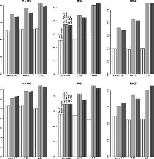
Figure 1: Average number of true positives for the Toeplitz model (top row) and the block model (bottom row). The number of hypotheses is increasing from $m=100$ (left panel) to $m=10\mbox{,}000$ (right panel) and the correlation parameter is varied as $\rho=0.95,0.975,0.99$ in the Toeplitz model and $\rho=0.6,0.75,0.9$ in the block model. The results are shown for the Bonferroni correction (single-step and corresponding step-down Bonferroni–Holm; light color); the oracle procedure (single-step and step-down; gray color) and the Westfall–Young permutation procedure (single-step and step-down; dark color).

We use a two-sided Wilcoxon test. The power over 250 simulations of the single-step and step-down methods of the Bonferroni-correction, the oracle procedure and the Westfall–Young permutation procedure are shown in Figure 1 for level $\alpha=0.05$. The step-down version of the Bonferroni correction is the Bonferroni–Holm procedure holm79simple and the step-down version of the Westfall–Young procedure is given in Westfall and Young westfall93resampling . The oracle threshold (both single-step and step-down) is approximated on a separate set of 1000 simulations, and the Westfall–Young method is using 1000 permutations for each simulation.

The following main results emerge: the Westfall–Young method is very close in power to the oracle procedure for all values of $m$ in the block model, giving support to the asymptotic results of Theorem 1. Moreover, the Westfall–Young and the oracle procedures are also very similar in the Toeplitz model, indicating that Theorem 1 may be generalized beyond block-independence models. The power gains of the Westfall–Young procedure, compared to Bonferroni–Holm, are substantial; between 20% and 250% for the considered scenarios, where the largest gains are achieved in settings with a large number of hypotheses and high correlations. Finally, the difference between step-down and single-step methods is very small in these sparse high-dimensional settings for all three multiple testing methods.

It might be unexpected that the power of the Westfall–Young is slightly larger than the oracle procedure for two settings with very high correlations. This is due to the finite number of simulations when approximating the oracle threshold, a finite number of permutations in the Westfall–Young procedure and a finite number of simulation runs. The family-wise error rate is between 0.03 and 0.04 for both oracle and Westfall–Young procedures and below 0.02 for the Bonferroni correction in the Toeplitz model. The nominal level of $\alpha=0.05$ is exceeded sometimes in the block model (again for the reason that we use only a finite number of simulations), where both the oracle and Westfall–Young procedures attain a family-wise error rate between 0.04 and 0.07 in all settings.

The computational cost of the Westfall–Young procedures scales approximately linearly with the number $m$ of hypotheses. When using 1000 permutations, computing the Westfall–Young threshold takes about 1.4 seconds per hypotheses on a 3 GHz CPU. For the largest setting of $m=10\mbox{,}000$ hypotheses, the threshold could thus be computed in just over 2 minutes. It seems as if this computational cost is acceptable, even for very large-scale testing problems.

5 Discussion

We considered asymptotic optimality of large-scale multiple testing under dependence within a nonparametric framework. We showed that, under certain assumptions, the Westfall–Young permutation method is asymptotically optimal in the following sense: with probability converging to 1 as the number of tests increases, the Westfall–Young critical value for multiple testing at nominal level $\alpha$ is greater than or equal to the unknown oracle threshold at level $\alpha-\delta$ for any $\delta>0$. This implies that the actual level of the Westfall–Young procedure converges to the effective oracle level $\alpha_{-}$. To investigate the possible impact of discrete $p$-values, we studied a specific example and provided sufficient conditions that ensure that $\alpha_{-}$ converges to $\alpha$.

We gave several examples that satisfy subset-pivotality and our assumptions (B1)–(B3) [while assumptions (A1)–(A3) are about the unknown data-generating distribution]. Most of these examples involve rank-based or permutation tests. These tests are appropriate for very high-dimensional testing problems. If the number of tests is in the thousands or even millions, extreme tail probabilities are required to claim significance, and these tail probabilities are more trustworthy under a nonparametric than a parametric test.

If the hypotheses are strongly dependent, the gain in power of the Westfall–Young method compared to a simple Bonferroni correction can be very substantial. This is a well known, empirical fact, and we have established here that this improvement is also optimal in the asymptotic framework we considered.

Our theoretical results could be expanded to include step-down procedures like Bonferroni–Holm holm79simple and the step-down Westfall–Young method westfall93resampling , GeEtAl03 . The distinction between single-step and step-down procedures is very marginal though in our sparse high-dimensional framework, as reported in Section 4, since the number of rejected hypotheses is orders of magnitudes smaller than the total number of hypotheses.

6 Proofs

After introducing some additional notation in Section 6.1, the proof of Theorem 1 is in Section 6.2 and the proof of Theorem 2 is in Section 6.3.

6.1 Additional notation

Let $p^{(b)}(W)$ be the minimum $p$-value over all true null hypotheses in the $b$th block:

$$p^{(b)}(W)=\min_{j\in A_{b}\cap I(P_{m})}p_{j}(W),\qquad b=1,\ldots,B,$$

and let $\pi_{b}(c)$ denote the probability under $P_{m}$ that $p^{(b)}(W)$ is less than or equal to a constant $c\in[0,1]$, that is,

$$\pi_{b}(c)=P_{m}\bigl{(}p^{(b)}(W)\leq c\bigr{)},\qquad b=1,\ldots,B.$$

Throughout, we denote the expected value, the variance and the covariance under $P_{m}$ by $E_{m}$, $\mathrm{Var}_{m}$ and $\mathrm{Cov}_{m}$, respectively.

6.2 Proof of Theorem 1

Let $\alpha^{\prime}\in(0,1)$ and $\delta^{\prime}\in(0,\alpha^{\prime})$. Let $\delta=\delta^{\prime}/2$ and $\alpha=\alpha^{\prime}-\delta^{\prime}$. Then writing expression (7) in terms of $\alpha^{\prime}$ and $\delta^{\prime}$ is equivalent to

$$P_{m}\{\hat{c}_{m,n}(\alpha+2\delta)\geq c_{m,n}(\alpha)\}\to 1\qquad\mbox{as }m\to\infty.$$

By definition,

$$\hat{c}_{m,n}(\alpha+2\delta)=\max\Bigl{\{}s\in S_{n}\dvtx P^{*}\Bigl{(}\min_{j\in\{1,\ldots,m\}}p_{j}(W)\leq s\Bigr{)}\leq\alpha+2\delta\Bigr{\}}.$$

We thus have to show that

$$P_{m}\Bigl{\{}P^{*}\Bigl{(}\min_{j\in\{1,\ldots,m\}}p_{j}(W)\leq c_{m,n}(\alpha)\Bigr{)}\leq\alpha+2\delta\Bigr{\}}\to 1$$ (9)

as $m\to\infty$.

First, we show in Lemma 1 that there exists an $M<\infty$ such that

$$P^{*}\Bigl{(}\min_{j\in\{1,\ldots,m\}}p_{j}(W)\leq c_{m,n}(\alpha)\Bigr{)}\leq P^{*}\Bigl{(}\min_{j\in I(P_{m})}p_{j}(W)\leq c_{m,n}(\alpha)\Bigr{)}+\delta$$

for all $m>M$ and for all $W$. This result is mainly due to the sparsity assumption (A2). Second, we show in Lemma 2 that

$$P_{m}\Bigl{\{}P^{*}\Bigl{(}\min_{j\in I(P_{m})}p_{j}(W)\leq c_{m,n}(\alpha)\Bigr{)}\leq\alpha+\delta\Bigr{\}}\to 1\qquad\mbox{for }m\to\infty.$$ (10)

Theorem 1 follows by combining these two results.

Lemma 1

Let $\alpha\in(0,1)$, $\delta\in(0,\alpha)$, and assume (A1), (A2), (B2)and (B3). Then there exists an $M<\infty$ such that

$$P^{*}\Bigl{(}\min_{j\in\{1,\ldots,m\}}p_{j}(W)\leq c_{m,n}(\alpha)\Bigr{)}\leq P^{*}\Bigl{(}\min_{j\in I(P_{m})}p_{j}(W)\leq c_{m,n}(\alpha)\Bigr{)}+\delta$$

for all $m>M$ and for all $W$.

Note that $c_{m,n}(\alpha)\in S_{n}$ by definition. Using the union bound, we have, for all $s\in S_{n}$ and all $W$,

$$P^{*}\Bigl{(}\min_{j\in\{1,\ldots,m\}}p_{j}(W)\leq s\Bigr{)} \leq P^{*}\Bigl{(}\min_{j\in I(P_{m})}p_{j}(W)\leq s\Bigr{)}$$

$${}+\sum_{j\in I^{\prime}(P_{m})}P^{*}\bigl{(}p_{j}(W)\leq s\bigr{)}.$$

Hence, we only need to show that there exists an $M<\infty$ such that

$$\sum_{j\in I^{\prime}(P_{m})}P^{*}\bigl{(}p_{j}(W)\leq c_{m,n}(\alpha)\bigr{)}\leq\delta$$ (12)

for all $m>M$ and all $W$. By assumption (B2) with constant $r$,

$$\sum_{j\in I^{\prime}(P_{m})}P^{*}\bigl{(}p_{j}(W)\leq c_{m,n}(\alpha)\bigr{)} \leq |I^{\prime}(P_{m})|rc_{m,n}(\alpha)$$

$$= r\frac{|I^{\prime}(P_{m})|}{B}Bc_{m,n}(\alpha).$$

Since $|I^{\prime}(P_{m})|/B\to 0$ as $m\to\infty$ by assumption (A2), and $Bc_{m,n}(\alpha)$ is bounded above by $-\log(1-\alpha)$ under assumptions (A1) and (B3) (see Lemma 3), we can choose a $M<\infty$ such that the right-hand side of (6.2) is bounded above by $\delta$ for all $m>M$. This proves the claim in (12) and completes the proof.

Lemma 2

Let $\alpha>0$ and $\delta>0$ and assume (A1), (A3) and (B1)–(B3). Then

$$P_{m}\Bigl{\{}P^{*}\Bigl{(}\min_{j\in I(P_{m})}p_{j}(W)\leq c_{m,n}(\alpha)\Bigr{)}\leq\alpha+\delta\Bigr{\}}\to 1\qquad\mbox{as }m\to\infty.$$

Let $\varepsilon>0$. The statement in the lemma is equivalent to showing that there exists an $M<\infty$ such that

$$P_{m}\Bigl{\{}P^{*}\Bigl{(}\min_{j\in I(P_{m})}p_{j}(W)>c_{m,n}(\alpha)\Bigr{)}<1-\alpha-\delta\Bigr{\}}<\varepsilon$$ (14)

for all $m>M$. By definition,

$$\quad P^{*}\Bigl{(}\min_{j\in I(P_{m})}p_{j}(W)>c_{m,n}(\alpha)\Bigr{)} = \frac{1}{|\mathcal{G}|}\sum_{g\in\mathcal{G}}1\Bigl{\{}\min_{j\in I(P_{m})}p_{j}(gW)>c_{m,n}(\alpha)\Bigr{\}}$$

$$= \frac{1}{|\mathcal{G}|}\sum_{g\in\mathcal{G}}R(g,W),$$

where

$$R(g,W):=1\Bigl{\{}\min_{j\in I(P_{m})}p_{j}(gW)>c_{m,n}(\alpha)\Bigr{\}}.$$

(We suppress the dependence on $m,n,P_{m}$ and $\alpha$ for notational simplicity.)

Let $G$ be a random permutation, chosen uniformly in $\mathcal{G}$, and let $1$ denote the identity permutation. Then, by assumption (B1), it follows that

$$E_{m}\biggl{(}\frac{1}{|\mathcal{G}|}\sum_{g\in\mathcal{G}}R(g,W)\biggr{)}=E_{m,G}R(G,W)=E_{m}R(1,W).$$

By definition of $c_{m,n}(\alpha)$ [see (1)],

$$E_{m}R(1,W)=P_{m}\Bigl{(}\min_{j\in I_{P_{m}}}p_{j}(W)>c_{m,n}(\alpha)\Bigr{)}\geq 1-\alpha.$$

Hence, the desired result (14) follows from a Markov inequality as soon as one can show that the variance of (6.2) vanishes as $m\to\infty$, that is, if

$$\mathrm{Var}_{m}\biggl{(}\frac{1}{|\mathcal{G}|}\sum_{g\in\mathcal{G}}R(g,W)\biggr{)}\,{=}\,\frac{1}{(|\mathcal{G}|)^{2}}\!\sum_{g,g^{\prime}\in\mathcal{G}}\!\mathrm{Cov}_{m}(R(g,W),R(g^{\prime},W))=o(1)$$ (16)

as $m\to\infty$.

Let $G,G^{\prime}$ be two random permutations, drawn independently and uniformly from $\mathcal{G}$. Then

$$\mathrm{Cov}_{m,G,G^{\prime}}(R(G,W),R(G^{\prime},W))=\frac{1}{(|\mathcal{G}|)^{2}}\sum_{g,g^{\prime}\in\mathcal{G}}\operatorname{Cov}_{m}(R(g,W),R(g^{\prime},W)).$$

Hence, in order to show (16), we only need to show that

$$\mathrm{Cov}_{m,G,G^{\prime}}(R(G,W),R(G^{\prime},W))=o(1)\qquad\mbox{for }m\to\infty.$$

Define

$$R_{b}(g,W):=1\bigl{\{}p^{(b)}(gW)>c_{m,n}(\alpha)\bigr{\}},$$ (17)

so that $R(g,W):=\prod_{b=1}^{B}R_{b}(g,W)$. We then need to prove that, as $m\to\infty$,

$$E_{m,G,G^{\prime}}\Biggl{(}\prod_{b=1}^{B}R_{b}(G,W)R_{b}(G^{\prime},W)\Biggr{)}\,{-}\,\Biggl{(}E_{m,G}\Biggl{(}\prod_{b=1}^{B}R_{b}(G,W)\Biggr{)}\Biggr{)}^{2}\,{=}\,o(1).$$ (18)

Using assumption (A1), the left-hand side in (18) can be written as

$$\prod_{b=1}^{B}E_{m,G,G^{\prime}}\{R_{b}(G,W)R_{b}(G^{\prime},W)\}-\prod_{b=1}^{B}[E_{m,G}\{R_{b}(G,W)\}]^{2}.$$

Note that $E_{m,G,G^{\prime}}\{R_{b}(G,W)R_{b}(G^{\prime},W)\}$ and $[E_{m,G}\{R_{b}(G,W)\}]^{2}$ are bounded between $0$ and $1$. For sequences of numbers $a_{1},\ldots,a_{B}$ and $b_{1},\ldots,b_{B}$ that are bounded between $0$ and $1$, the following inequality holds:

$$\Biggl{|}\prod_{j=1}^{B}a_{j}-\prod_{j=1}^{B}b_{j}\Biggr{|}=\Biggl{|}\sum_{j=1}^{B}\biggl{\{}(a_{j}-b_{j})\biggl{(}\prod_{k<j}b_{k}\biggr{)}\biggl{(}\prod_{k>j}a_{k}\biggr{)}\biggr{\}}\Biggr{|}\leq\sum_{j=1}^{B}|a_{j}-b_{j}|.$$

Hence, in order to show (18) it is sufficient to show that

$${\max_{b=1,\ldots,B}}|E_{m,G,G^{\prime}}\{R_{b}(G,W)R_{b}(G^{\prime},W)\}-[E_{m,G}\{R_{b}(G,W)\}]^{2}|$$

(19)

$$\qquad=o(B^{-1})$$

as $m\to\infty$.

Conditional on $W$,

$$R_{b}(G,W),R_{b}(G^{\prime},W)\stackrel{{\scriptstyle\mathrm{i.i.d.}}}{{\sim}}\operatorname{Bernoulli}(\mu_{b}(W)),$$

where $\mu_{b}(W)$ is the proportion of all permutations $g\in\mathcal{G}$ for which $R_{b}(g,W)=1$ or, equivalently,

$$\mu_{b}(W)=P_{m,G}\bigl{\{}p^{(b)}(GW)>c_{m,n}(\alpha)|W\bigr{\}}=P^{*}\bigl{\{}p^{(b)}(W)>c_{m,n}(\alpha)\bigr{\}}.$$ (20)

Thus, the random proportion $\mu_{b}(W)$ is a function of $W$. Denote its distribution by $F_{b}$. Using Lemma 4, the support of $F_{b}$ is contained in the interval $[1-\log\{1/(1-\alpha)\}\alpha r^{2}m_{B}B^{-1},1]$ under assumptions (A1), (B1) and (B2). Hence, using Lemma 5, it follows that

$$0 \leq E_{m,G,G^{\prime}}\{R_{b}(G,W)R_{b}(G^{\prime},W)\}-[E_{m,G}\{R_{b}(G,W)\}]^{2}$$

$$\leq \bigl{(}\log\{1/(1-\alpha)\}\alpha r^{2}m_{B}B^{-1}\bigr{)}^{2}.$$

Since $m_{B}=o(\sqrt{B})$ under assumption (A3), claim (6.2) follows.

Lemma 3

Under assumptions (A1) and (B3), we have

$$Bc_{m,n}(\alpha)\leq\sum_{b=1}^{B}\pi_{b}(c_{m,n}(\alpha))\leq\log\{1/(1-\alpha)\}.$$ (21)

Let $b\in\{1,\ldots,B\}$ and $j_{b}\in I(P_{m})\cap A_{b}$. Then

$$\pi_{b}\{c_{m,n}(\alpha)\}\geq P_{m}\bigl{(}p_{j_{b}}(W)\leq c_{m,n}(\alpha)\bigr{)}=c_{m,n}(\alpha),$$ (22)

where the inequality follows from the definition of $\pi_{b}(\cdot)$, and the equality follows from assumption (B3) and the fact that $c_{m,n}(\alpha)\in S_{n}$. Summing (22) over $b=1,\ldots,B$ yields the first inequality of (21).

To prove the second inequality of (21), note that assumption (A1) and the definition of $c_{m,n}(\alpha)$ imply that

$$1-\prod_{b=1}^{B}[1-\pi_{b}\{c_{m,n}(\alpha)\}]\leq\alpha.$$ (23)

The maximum of $\sum_{b=1}^{B}\pi_{b}\{c_{m,n}(\alpha)\}$ under constraint (23) is obtained when

$$\pi_{1}\{c_{m,n}(\alpha)\}=\cdots=\pi_{B}\{c_{m,n}(\alpha)\}.$$

This implies $\pi_{b}\{c_{m,n}(\alpha)\}\leq 1-(1-\alpha)^{1/B}$ for all $b=1,\ldots,B$, so that

$$\sum_{b=1}^{B}\pi_{b}\{c_{m,n}(\alpha)\}\leq B-B(1-\alpha)^{1/B},$$

and this is bounded above by $-\log(1-\alpha)$ for all values of $B$.

Lemma 4

Assume (A1), (B1) and (B2). Let $F_{b}$ be the distribution of $\mu_{b}(W)$, where $\mu_{b}(W)$ is defined in (20). Then

$$\operatorname{support}(F_{b})\subseteq[1-\log\{1/(1-\alpha)\}\alpha r^{2}m_{B}B^{-1},1].$$

Using assumption (B2) with constant $r$ and the union bound, it holds that

$$1-\mu_{b}(W)=P^{*}\bigl{\{}p^{(b)}(W)\leq c_{m,n}(\alpha)\bigr{\}}\leq r|A_{b}|c_{m,n}(\alpha).$$

Since $m_{B}=\max_{b=1,\ldots,B}|A_{b}|$, the support of $F_{b}$ is thus in the interval $[1-m_{B}rc_{m,n}(\alpha),1]$.

Hence, the proof is complete if we show that

$$c_{m,n}(\alpha)\leq-\log(1-\alpha)\alpha rB^{-1}.$$ (24)

To see that (24) holds, we first show that

$$1-\alpha\leq P_{m}\Bigl{\{}\min_{j\in I(P_{m})}p_{j}(W)>c_{m,n}(\alpha)\Bigr{\}}\leq\bigl{(}1-c_{m,n}(\alpha)/r\bigr{)}^{B}.$$ (25)

The first inequality in (25) follows directly from the definition of $c_{m,n}(\alpha)$; see (1). To prove the second inequality, note that assumption (A1) implies that

$$P_{m}\Bigl{\{}\min_{j\in I(P_{m})}p_{j}(W)>c_{m,n}(\alpha)\Bigr{\}}=\prod_{b=1}^{B}P_{m}\bigl{\{}p^{(b)}(W)>c_{m,n}(\alpha)\bigr{\}}.$$ (26)

By assumption (B1) and the law of iterated expectations,

$$P_{m}\bigl{\{}p^{(b)}(W)>c_{m,n}(\alpha)\bigr{\}} = P_{m,G}\bigl{\{}p^{(b)}(GW)>c_{m,n}(\alpha)\bigr{\}}$$

$$= E_{m}\bigl{\{}P_{m,G}\bigl{\{}p^{(b)}(GW)>c_{m,n}(\alpha)|W\bigr{\}}\bigr{\}}.$$

By assumption (B2), the conditional probability within each block satisfies

$$P_{m,G}\bigl{\{}p^{(b)}(GW)>c_{m,n}(\alpha)|W\bigr{\}} = P^{*}\bigl{\{}p^{(b)}(W)>c_{m,n}(\alpha)\bigr{\}}$$

$$\leq 1-P^{*}\{p_{j_{b}}(W)\leq c_{m,n}(\alpha)\}$$

$$\leq 1-c_{m,n}(\alpha)/r,$$

where $j_{b}\in I(P_{m})\cap A_{b}$. Since the right-hand side of (6.2) does not depend on $W$, the same bound holds for (6.2), where we also take the expectation over $W$. Using this result in (26), the second inequality in (25) follows. Finally, (25) implies

$$c_{m,n}(\alpha)\leq r\{1-(1-\alpha)^{1/B}\}.$$

Since $B(1-(1-\alpha)^{1/B})\leq-\log(1-\alpha)$ for all values of $B$, it follows that $1-(1-\alpha)^{1/B}\leq-\log(1-\alpha)B^{-1}$. This proves (24) and completes the proof. 

Lemma 5

Let $U$ be a real-valued random variable with support $[a,b]\subset[0,1]$. Suppose that the distribution of the two random variables $X_{1}$ and $X_{2}$, conditional on $U=u$, is given by

$$X_{1},X_{2}\stackrel{{\scriptstyle\mathrm{i.i.d.}}}{{\sim}}\operatorname{Bernoulli}(u).$$

Then $0\leq E(X_{1}X_{2})-E(X_{1})E(X_{2})\leq(b-a)^{2}$.

By the assumption that $X_{1}$ and $X_{2}$ are Bernoulli conditional on $U$, it follows that $E(X_{1}|U)=E(X_{2}|U)=U$. Combining this with the law of iterated expectation and the fact that $X_{1}$ and $X_{2}$ are conditionally independent given $U$, we obtain

$$E(X_{1}X_{2})=E_{U}\{E(X_{1}X_{2}|U)\}=E_{U}\{E(X_{1}|U)E(X_{2}|U)\}=E(U^{2}).$$

Moreover, we have $E(X_{1})=E_{U}\{E(X_{1}|U)\}=E(U)$ and similarly $E(X_{2})=E(U)$. Hence,

$$E(X_{1}X_{2})-E(X_{1})E(X_{2})=E(U^{2})-\{E(U)\}^{2}=\operatorname{Var}(U).$$

Finally, $0\leq\operatorname{Var}(U)\leq(b-a)^{2}$ by the assumption on the support of $U$.

6.3 Proof of Theorem 2

First, note that (W) implies (B1)–(B3). Using the union bound and assumption (B3), it holds for any $s\in S_{n}$ that $ms$ is an upper bound for $P_{m}(\min_{j\in I(P_{m})}p_{j}(W)\leq s)$. Hence,

$$c_{m,n}(\alpha) = \max\Bigl{\{}s\in S_{n}\dvtx P_{m}\Bigl{(}\min_{j\in I(P_{m})}p_{j}(W)\leq s\Bigr{)}\leq\alpha\Bigr{\}}$$

$$\geq \max\{s\in S_{n}\dvtx ms\leq\alpha\}.$$

This implies that the oracle critical value is larger than zero if the set $\{s\in S_{n}\dvtx ms\leq\alpha\}$ is nonempty, which is the case if $\min(S_{n})\leq\alpha/m$. The smallest possible two-sided Wilcoxon $p$-value is $\min(S_{n})=2\frac{(n/2)!(n/2)!}{n!}\leq 2^{-n/2+1}$. Hence, it is sufficient to require that $2^{-n/2+1}\leq\alpha/m$, or equivalently, that $n\geq 2\log_{2}(m/\alpha)+2$.

Note that (A3^′) implies (A3). Hence, under assumptions (W), (A1), (A2) and (A3^′), the result in Theorem 1 applies.

Let $\alpha\in(0,1)$. We will now show that under assumptions (W), (A1) and (A3^′),

$$\alpha_{-}\to\alpha$$

as $m,n\to\infty$ such that $n/\log(m)\to\infty$, where $\alpha_{-}$ was defined in (8). Define $c^{+}_{m,n}(\alpha):=\min\{s\in S_{n}\dvtx s>c_{m,n}(\alpha)\}$. Using the definition of $\alpha_{-}$ and assumption (A1), we have

$$\alpha_{-} = P_{m}\Bigl{(}\min_{j\in I(P_{m})}p_{j}(W)\leq c_{m,n}(\alpha)\Bigr{)}$$

$$= 1-\prod_{b=1}^{B}[1-\pi_{b}\{c_{m,n}(\alpha)\}]$$

$$= 1-\prod_{b=1}^{B}[1-\pi_{b}\{c^{+}_{m,n}(\alpha)\}+\pi_{b}\{c^{+}_{m,n}(\alpha)\}-\pi_{b}\{c_{m,n}(\alpha)\}].$$

Define the function $g_{m,n}\dvtx\prod_{b=1}^{B}[0,\pi_{b}\{c_{m,n}^{+}(\alpha)\}]\to\mathbb{R}$ by

$$g_{m,n}(u) := g_{m,n}(u_{1},\ldots,u_{B})$$

$$:= 1-\prod_{b=1}^{B}[1-\pi_{b}\{c^{+}_{m,n}(\alpha)\}+u_{b}],$$

so that the right-hand side of (6.3) equals $g_{m,n}(w)$, where $w_{b}:=\pi_{b}\{c^{+}_{m,n}(\alpha)\}-\pi_{b}\{c_{m,n}(\alpha)\}$ for $b=1,\ldots,B$. A first-order Taylor expansion of $g_{m,n}(w)$ around $(0,\ldots,0)$ yields

$$\alpha_{-}=g_{m,n}(w)=g_{m,n}(0)+\sum_{b=1}^{B}w_{b}\,\frac{\partial g_{m,n}(u)}{\partial u_{b}}\bigg{|}_{u=0}+R,$$ (31)

where $R=o(\sum_{b=1}^{B}w_{b})$. For all $b=1,\ldots,B$, we have

$$\frac{\partial g_{m,n}(u)}{\partial u_{b}}\bigg{|}_{u=0} = -\prod_{j=1,j\neq b}^{B}[1-\pi_{j}\{c^{+}_{m,n}(\alpha)\}]$$

$$= -\frac{1-g_{m,n}(0)}{1-\pi_{b}\{c^{+}_{m,n}(\alpha)\}}\geq-\frac{1-g_{m,n}(0)}{1-m_{B}c^{+}_{m,n}(\alpha)},$$

where the inequality follows from $\pi_{b}\{c^{+}_{m,n}(\alpha)\}\leq m_{B}c^{+}_{m,n}(\alpha)$ for $b=1,\ldots,B$, by the union bound and assumption (B3). Plugging this into (31) yields

$$\alpha_{-} \geq g_{m,n}(0)-\frac{1-g_{m,n}(0)}{1-m_{B}c^{+}_{m,n}(\alpha)}\sum_{b=1}^{B}w_{b}+R$$

$$= g_{m,n}(0)\biggl{(}1+\frac{\sum_{b=1}^{B}w_{b}}{1-m_{B}c^{+}_{m,n}(\alpha)}\biggr{)}-\frac{\sum_{b=1}^{B}w_{b}}{1-m_{B}c^{+}_{m,n}(\alpha)}+R.$$

The definition of $c^{+}_{m,n}(\alpha)$ implies that $g_{m,n}(0)>\alpha$ for all $m$ and $n$. Hence, if

$$\sum_{b=1}^{B}w_{b}\to 0\quad\mbox{and}\quad m_{B}c^{+}_{m,n}(\alpha)\to 0$$ (33)

as $m,n\to\infty$ such that $n/\log(m)\to\infty$, then the right-hand side of (6.3) converges to $\alpha$ and the proof is complete.

We first consider $\sum_{b=1}^{B}w_{b}$. By definition, there is no value $s^{\prime}\in S_{n}$ such that $c_{m,n}(\alpha)<s^{\prime}<c^{+}_{m,n}(\alpha)$. Hence,

$$w_{b} = P_{m}\Bigl{\{}\min_{j\in A_{b}\cap I(P_{m})}p_{j}(W)=c^{+}_{m,n}(\alpha)\Bigr{\}}$$

$$\leq m_{B}\max_{j\in A_{b}\cap I(P_{m})}P_{m}\{p_{j}(W)=c^{+}_{m,n}(\alpha)\}$$

$$= m_{B}\{c^{+}_{m,n}(\alpha)-c_{m,n}(\alpha)\},$$

where the inequality follows from the union bound, and the last equality is due to assumption (B3). This implies

$$\sum_{b=1}^{B}w_{b}\leq Bm_{B}\{c^{+}_{m,n}(\alpha)-c_{m,n}(\alpha)\}=Bc_{m,n}(\alpha)m_{B}\biggl{(}\frac{c^{+}_{m,n}(\alpha)}{c_{m,n}(\alpha)}-1\biggr{)}.$$

Similarly, we have

$$m_{B}c^{+}_{m,n}(\alpha)=Bc_{m,n}(\alpha)\frac{m_{B}}{B}\frac{c^{+}_{m,n}(\alpha)}{c_{m,n}(\alpha)}.$$

Note that $Bc_{m,n}(\alpha)\leq\log\{1/(1-\alpha)\}$ by Lemma 3 and $m_{B}=O(1)$ (and hence $B\to\infty$) by assumption (A3^′). Hence, in order to prove (33), it suffices to show that

$$c_{m,n}^{+}(\alpha)/c_{m,n}(\alpha)\to 1\qquad\mbox{as }m,n\to\infty,n/\log(m)\to\infty.$$ (34)

Let the ordered $p$-values in $S_{n}$, based on a two-sided Wilcoxon test with equal sample sizes $n/2$ in both classes, be denoted by $s_{0}<s_{1}<\cdots<s_{r_{n}}$, where $r_{n}=\lfloor n^{2}/8+1\rfloor$. It is well known that

$$s_{i}=2\frac{(n/2)!(n/2)!}{n!}\sum_{j=0}^{i}q_{n/2}(j)\qquad\mbox{for }i=0,\ldots,r_{n}-1$$

and $s_{r_{n}}=1$, where $q_{n}(j)$ is the number of integer partitions of $j$ such that neither the number of parts nor the part magnitudes exceed $n$ [and $q_{n}(0)\,{=}\,1$] Wilcoxon45 . Let $i_{m,n}$ satisfy $s_{i_{m,n}}=c_{m,n}(\alpha)$. Then

$$\frac{c^{+}_{m,n}(\alpha)}{c_{m,n}(\alpha)}=\frac{\sum_{j=0}^{i_{m,n}+1}q_{n/2}(j)}{\sum_{j=0}^{i_{m,n}}q_{n/2}(j)}.$$

This ratio converges to 1 if $i_{m,n}\to\infty$. Recall that $c_{m,n}(\alpha)\geq\max\{s\in S_{n}\dvtx s\leq\alpha/m\}$ [see (6.3)]. Hence,

$$c^{+}_{m,n}(\alpha)=2\frac{(n/2)!(n/2)!}{n!}\sum_{j=0}^{i_{m,n}+1}q_{n/2}(j)>\alpha/m.$$

Since $2m\{(n/2)!(n/2)!\}/n!\leq m2^{-n/2}\to 0$ as $m,n\to\infty$ such that $n/\break\log(m)\to\infty$, we have that under these conditions $i_{m,n}\to\infty$ and $c^{+}_{m,n}(\alpha)/\break c_{m,n}(\alpha)\to 1$. Thus (34) holds and hence implies (33), which completes the proof.

References

- (1) {barticle}[auto:STB—2011/12/30—12:36:46] \bauthor\bsnmBecker, \bfnmT.\binitsT. and \bauthor\bsnmKnapp, \bfnmM.\binitsM. (\byear2004). \btitleA powerful strategy to account for multiple testing in the context of haplotype analysis. \bjournalThe American Journal of Human Genetics \bvolume75 \bpages561–570. \bptokimsref \endbibitem
- (2) {barticle}[mr] \bauthor\bsnmBenjamini, \bfnmYoav\binitsY., \bauthor\bsnmKrieger, \bfnmAbba M.\binitsA. M. and \bauthor\bsnmYekutieli, \bfnmDaniel\binitsD. (\byear2006). \btitleAdaptive linear step-up procedures that control the false discovery rate. \bjournalBiometrika \bvolume93 \bpages491–507. \biddoi=10.1093/biomet/93.3.491, issn=0006-3444, mr=2261438 \bptokimsref \endbibitem
- (3) {barticle}[mr] \bauthor\bsnmBenjamini, \bfnmYoav\binitsY. and \bauthor\bsnmYekutieli, \bfnmDaniel\binitsD. (\byear2001). \btitleThe control of the false discovery rate in multiple testing under dependency. \bjournalAnn. Statist. \bvolume29 \bpages1165–1188. \biddoi=10.1214/aos/1013699998, issn=0090-5364, mr=1869245 \bptokimsref \endbibitem
- (4) {barticle}[mr] \bauthor\bsnmBlanchard, \bfnmGilles\binitsG. and \bauthor\bsnmRoquain, \bfnmÉtienne\binitsÉ. (\byear2009). \btitleAdaptive false discovery rate control under independence and dependence. \bjournalJ. Mach. Learn. Res. \bvolume10 \bpages2837–2871. \bidissn=1532-4435, mr=2579914 \bptokimsref \endbibitem
- (5) {barticle}[auto:STB—2011/12/30—12:36:46] \bauthor\bsnmBond, \bfnmG. L.\binitsG. L., \bauthor\bsnmHu, \bfnmW.\binitsW. and \bauthor\bsnmLevine, \bfnmA.\binitsA. (\byear2005). \btitleA single nucleotide polymorphism in the MDM2 gene: From a molecular and cellular explanation to clinical effect. \bjournalCancer Research \bvolume65 \bpages5481–5484. \bptokimsref \endbibitem
- (6) {barticle}[auto:STB—2011/12/30—12:36:46] \bauthor\bsnmCheung, \bfnmV. G.\binitsV. G., \bauthor\bsnmSpielman, \bfnmR. S.\binitsR. S., \bauthor\bsnmEwens, \bfnmK. G.\binitsK. G., \bauthor\bsnmWeber, \bfnmT. M.\binitsT. M., \bauthor\bsnmMorley, \bfnmM.\binitsM. and \bauthor\bsnmBurdick, \bfnmJ. T.\binitsJ. T. (\byear2005). \btitleMapping determinants of human gene expression by regional and genome-wide association. \bjournalNature \bvolume437 \bpages1365–1369. \bptokimsref \endbibitem
- (7) {barticle}[mr] \bauthor\bsnmClarke, \bfnmSandy\binitsS. and \bauthor\bsnmHall, \bfnmPeter\binitsP. (\byear2009). \btitleRobustness of multiple testing procedures against dependence. \bjournalAnn. Statist. \bvolume37 \bpages332–358. \biddoi=10.1214/07-AOS557, issn=0090-5364, mr=2488354 \bptokimsref \endbibitem
- (8) {barticle}[mr] \bauthor\bsnmDudoit, \bfnmSandrine\binitsS., \bauthor\bsnmShaffer, \bfnmJuliet Popper\binitsJ. P. and \bauthor\bsnmBoldrick, \bfnmJennifer C.\binitsJ. C. (\byear2003). \btitleMultiple hypothesis testing in microarray experiments. \bjournalStatist. Sci. \bvolume18 \bpages71–103. \biddoi=10.1214/ss/1056397487, issn=0883-4237, mr=1997066 \bptokimsref \endbibitem
- (9) {bbook}[mr] \bauthor\bsnmDudoit, \bfnmSandrine\binitsS. and \bauthor\bparticlevan der \bsnmLaan, \bfnmMark J.\binitsM. J. (\byear2008). \btitleMultiple Testing Procedures with Applications to Genomics. \bpublisherSpringer, \baddressNew York. \biddoi=10.1007/978-0-387-49317-6, mr=2373771 \bptokimsref \endbibitem
- (10) {barticle}[mr] \bauthor\bsnmEfron, \bfnmBradley\binitsB. (\byear2007). \btitleCorrelation and large-scale simultaneous significance testing. \bjournalJ. Amer. Statist. Assoc. \bvolume102 \bpages93–103. \biddoi=10.1198/016214506000001211, issn=0162-1459, mr=2293302 \bptokimsref \endbibitem
- (11) {barticle}[mr] \bauthor\bsnmGe, \bfnmYongchao\binitsY., \bauthor\bsnmDudoit, \bfnmSandrine\binitsS. and \bauthor\bsnmSpeed, \bfnmTerence P.\binitsT. P. (\byear2003). \btitleResampling-based multiple testing for microarray data analysis. \bjournalTest \bvolume12 \bpages1–77. \biddoi=10.1007/BF02595811, issn=1133-0686, mr=1993286 \bptokimsref \endbibitem
- (12) {barticle}[mr] \bauthor\bsnmGenovese, \bfnmChristopher R.\binitsC. R., \bauthor\bsnmRoeder, \bfnmKathryn\binitsK. and \bauthor\bsnmWasserman, \bfnmLarry\binitsL. (\byear2006). \btitleFalse discovery control with -value weighting. \bjournalBiometrika \bvolume93 \bpages509–524. \biddoi=10.1093/biomet/93.3.509, issn=0006-3444, mr=2261439 \bptokimsref \endbibitem
- (13) {barticle}[mr] \bauthor\bsnmGoeman, \bfnmJelle J.\binitsJ. J. and \bauthor\bsnmSolari, \bfnmAldo\binitsA. (\byear2010). \btitleThe sequential rejection principle of familywise error control. \bjournalAnn. Statist. \bvolume38 \bpages3782–3810. \biddoi=10.1214/10-AOS829, issn=0090-5364, mr=2766868 \bptokimsref \endbibitem
- (14) {bmisc}[auto:STB—2011/12/30—12:36:46] \bauthor\bsnmGood, \bfnmP. I.\binitsP. I. (\byear2011). \bhowpublishedPermutation tests. In Analyzing the Large Number of Variables in Biomedical and Satellite Imagery 5–20. Wiley, Hoboken, NJ. \bptokimsref \endbibitem
- (15) {barticle}[auto:STB—2011/12/30—12:36:46] \bauthor\bsnmGoode, \bfnmE. L.\binitsE. L., \bauthor\bsnmDunning, \bfnmA. M.\binitsA. M., \bauthor\bsnmKuschel, \bfnmB.\binitsB., \bauthor\bsnmHealey, \bfnmC. S.\binitsC. S., \bauthor\bsnmDay, \bfnmN. E.\binitsN. E., \bauthor\bsnmPonder, \bfnmB. A. J.\binitsB. A. J., \bauthor\bsnmEaston, \bfnmD. F.\binitsD. F. and \bauthor\bsnmPharoah, \bfnmP. P. D.\binitsP. P. D. (\byear2002). \btitleEffect of germ-line genetic variation on breast cancer survival in a population-based study. \bjournalCancer Research \bvolume62 \bpages3052–3057. \bptokimsref \endbibitem
- (16) {barticle}[mr] \bauthor\bsnmHall, \bfnmPeter\binitsP. and \bauthor\bsnmJin, \bfnmJiashun\binitsJ. (\byear2008). \btitleProperties of higher criticism under strong dependence. \bjournalAnn. Statist. \bvolume36 \bpages381–402. \biddoi=10.1214/009053607000000767, issn=0090-5364, mr=2387976 \bptokimsref \endbibitem
- (17) {barticle}[mr] \bauthor\bsnmHall, \bfnmPeter\binitsP. and \bauthor\bsnmJin, \bfnmJiashun\binitsJ. (\byear2010). \btitleInnovated higher criticism for detecting sparse signals in correlated noise. \bjournalAnn. Statist. \bvolume38 \bpages1686–1732. \biddoi=10.1214/09-AOS764, issn=0090-5364, mr=2662357 \bptokimsref \endbibitem
- (18) {barticle}[auto:STB—2011/12/30—12:36:46] \bauthor\bsnmHirschhorn, \bfnmJ. N.\binitsJ. N. and \bauthor\bsnmDaly, \bfnmM. J.\binitsM. J. (\byear2005). \btitleGenome-wide association studies for common diseases and complex traits. \bjournalNature Reviews Genetics \bvolume6 \bpages95–108. \bptokimsref \endbibitem
- (19) {barticle}[mr] \bauthor\bsnmHolm, \bfnmSture\binitsS. (\byear1979). \btitleA simple sequentially rejective multiple test procedure. \bjournalScand. J. Stat. \bvolume6 \bpages65–70. \bidissn=0303-6898, mr=0538597 \bptokimsref \endbibitem
- (20) {barticle}[auto:STB—2011/12/30—12:36:46] \bauthor\bsnmKruglyak, \bfnmL.\binitsL. (\byear1999). \btitleProspects for whole-genome linkage disequilibrium mapping of common disease genes. \bjournalNature Genetics \bvolume22 \bpages139–144. \bptokimsref \endbibitem
- (21) {barticle}[mr] \bauthor\bsnmLiang, \bfnmChyng-Lan\binitsC.-L., \bauthor\bsnmRice, \bfnmJohn A.\binitsJ. A., \bauthor\bparticlede \bsnmPater, \bfnmImke\binitsI., \bauthor\bsnmAlcock, \bfnmCharles\binitsC., \bauthor\bsnmAxelrod, \bfnmTim\binitsT., \bauthor\bsnmWang, \bfnmAndrew\binitsA. and \bauthor\bsnmMarshall, \bfnmStuart\binitsS. (\byear2004). \btitleStatistical methods for detecting stellar occultations by Kuiper belt objects: The Taiwanese–American occultation survey. \bjournalStatist. Sci. \bvolume19 \bpages265–274. \biddoi=10.1214/088342304000000378, issn=0883-4237, mr=2146947 \bptnotecheck year\bptokimsref \endbibitem
- (22) {barticle}[auto:STB—2011/12/30—12:36:46] \bauthor\bsnmLudbrook, \bfnmJ.\binitsJ. and \bauthor\bsnmDudley, \bfnmH.\binitsH. (\byear1998). \btitleWhy permutation tests are superior to and tests in biomedical research. \bjournalAmer. Statist. \bvolume52 \bpages127–132. \bptokimsref \endbibitem
- (23) {barticle}[auto:STB—2011/12/30—12:36:46] \bauthor\bsnmMarchini, \bfnmJ.\binitsJ., \bauthor\bsnmDonnelly, \bfnmP.\binitsP. and \bauthor\bsnmCardon, \bfnmL. R.\binitsL. R. (\byear2005). \btitleGenome-wide strategies for detecting multiple loci that influence complex diseases. \bjournalNature Genetics \bvolume37 \bpages413–417. \bptokimsref \endbibitem
- (24) {barticle}[auto:STB—2011/12/30—12:36:46] \bauthor\bsnmMcCarthy, \bfnmM. I.\binitsM. I., \bauthor\bsnmAbecasis, \bfnmG. R.\binitsG. R., \bauthor\bsnmCardon, \bfnmL. R.\binitsL. R., \bauthor\bsnmGoldstein, \bfnmD. B.\binitsD. B., \bauthor\bsnmLittle, \bfnmJ.\binitsJ., \bauthor\bsnmIoannidis, \bfnmJ. P. A.\binitsJ. P. A. and \bauthor\bsnmHirschhorn, \bfnmJ. N.\binitsJ. N. (\byear2008). \btitleGenome-wide association studies for complex traits: Consensus, uncertainty and challenges. \bjournalNature Reviews Genetics \bvolume9 \bpages356–369. \bptokimsref \endbibitem
- (25) {barticle}[mr] \bauthor\bsnmMeinshausen, \bfnmNicolai\binitsN. (\byear2006). \btitleFalse discovery control for multiple tests of association under general dependence. \bjournalScand. J. Stat. \bvolume33 \bpages227–237. \biddoi=10.1111/j.1467-9469.2005.00488.x, issn=0303-6898, mr=2279639 \bptokimsref \endbibitem
- (26) {barticle}[mr] \bauthor\bsnmMeinshausen, \bfnmNicolai\binitsN. and \bauthor\bsnmRice, \bfnmJohn\binitsJ. (\byear2006). \btitleEstimating the proportion of false null hypotheses among a large number of independently tested hypotheses. \bjournalAnn. Statist. \bvolume34 \bpages373–393. \biddoi=10.1214/009053605000000741, issn=0090-5364, mr=2275246 \bptokimsref \endbibitem
- (27) {barticle}[auto:STB—2011/12/30—12:36:46] \bauthor\bsnmReiner, \bfnmA.\binitsA., \bauthor\bsnmYekutieli, \bfnmD.\binitsD. and \bauthor\bsnmBenjamini, \bfnmY.\binitsY. (\byear2003). \btitleIdentifying differentially expressed genes using false discovery rate controlling procedures. \bjournalBioinformatics \bvolume19 \bpages368–375. \bptokimsref \endbibitem
- (28) {barticle}[mr] \bauthor\bsnmRoeder, \bfnmKathryn\binitsK. and \bauthor\bsnmWasserman, \bfnmLarry\binitsL. (\byear2009). \btitleGenome-wide significance levels and weighted hypothesis testing. \bjournalStatist. Sci. \bvolume24 \bpages398–413. \biddoi=10.1214/09-STS289, issn=0883-4237, mr=2779334 \bptokimsref \endbibitem
- (29) {barticle}[mr] \bauthor\bsnmRomano, \bfnmJoseph P.\binitsJ. P. and \bauthor\bsnmWolf, \bfnmMichael\binitsM. (\byear2005). \btitleExact and approximate stepdown methods for multiple hypothesis testing. \bjournalJ. Amer. Statist. Assoc. \bvolume100 \bpages94–108. \biddoi=10.1198/016214504000000539, issn=0162-1459, mr=2156821 \bptokimsref \endbibitem
- (30) {barticle}[mr] \bauthor\bsnmSun, \bfnmWenguang\binitsW. and \bauthor\bsnmCai, \bfnmT. Tony\binitsT. T. (\byear2009). \btitleLarge-scale multiple testing under dependence. \bjournalJ. R. Stat. Soc. Ser. B Stat. Methodol. \bvolume71 \bpages393–424. \biddoi=10.1111/j.1467-9868.2008.00694.x, issn=1369-7412, mr=2649603 \bptokimsref \endbibitem
- (31) {barticle}[mr] \bauthor\bsnmWestfall, \bfnmPeter H.\binitsP. H. and \bauthor\bsnmTroendle, \bfnmJames F.\binitsJ. F. (\byear2008). \btitleMultiple testing with minimal assumptions. \bjournalBiom. J. \bvolume50 \bpages745–755. \biddoi=10.1002/bimj.200710456, issn=0323-3847, mr=2542340 \bptokimsref \endbibitem
- (32) {barticle}[mr] \bauthor\bsnmWestfall, \bfnmPeter H.\binitsP. H. and \bauthor\bsnmYoung, \bfnmS. Stanley\binitsS. S. (\byear1989). \btitle-value adjustments for multiple tests in multivariate binomial models. \bjournalJ. Amer. Statist. Assoc. \bvolume84 \bpages780–786. \bidissn=0162-1459, mr=1132592 \bptokimsref \endbibitem
- (33) {bbook}[auto:STB—2011/12/30—12:36:46] \bauthor\bsnmWestfall, \bfnmP. H.\binitsP. H. and \bauthor\bsnmYoung, \bfnmS. S.\binitsS. S. (\byear1993). \btitleResampling-Based Multiple Testing: Examples and Methods for -Value Adjustment. \bpublisherWiley, \baddressNew York. \bptokimsref \endbibitem
- (34) {bincollection}[auto:STB—2011/12/30—12:36:46] \bauthor\bsnmWestfall, \bfnmP. H.\binitsP. H., \bauthor\bsnmZaykin, \bfnmD. V.\binitsD. V. and \bauthor\bsnmYoung, \bfnmS. S.\binitsS. S. (\byear2002). \btitleMultiple tests for genetic effects in association studies. In \bbooktitleBiostatistical Methods: Methods in Molecular Biology (\beditor\bfnmS.\binitsS. \bsnmLooney, ed.) \bvolume184 \bpages143–168. \bpublisherHumana Press, \baddressTotawa, NJ. \bptokimsref \endbibitem
- (35) {barticle}[auto:STB—2011/12/30—12:36:46] \bauthor\bsnmWilcoxon, \bfnmF.\binitsF. (\byear1945). \btitleIndividual comparisons by ranking methods. \bjournalBiometrics Bulletin \bvolume1 \bpages80–83. \bptokimsref \endbibitem
- (36) {barticle}[auto:STB—2011/12/30—12:36:46] \bauthor\bsnmWinkelmann, \bfnmJ.\binitsJ., \bauthor\bsnmSchormair, \bfnmB.\binitsB., \bauthor\bsnmLichtner, \bfnmP.\binitsP., \bauthor\bsnmRipke, \bfnmS.\binitsS., \bauthor\bsnmXiong, \bfnmL.\binitsL., \bauthor\bsnmJalilzadeh, \bfnmS.\binitsS., \bauthor\bsnmFulda, \bfnmS.\binitsS., \bauthor\bsnmPütz, \bfnmB.\binitsB., \bauthor\bsnmEckstein, \bfnmG.\binitsG. and \bauthor\bsnmHauk, \bfnmS.\binitsS. et al. (\byear2007). \btitleGenome-wide association study of restless legs syndrome identifies common variants in three genomic regions. \bjournalNature Genetics \bvolume39 \bpages1000–1006. \bptokimsref \endbibitem
- (37) {barticle}[mr] \bauthor\bsnmYekutieli, \bfnmDaniel\binitsD. and \bauthor\bsnmBenjamini, \bfnmYoav\binitsY. (\byear1999). \btitleResampling-based false discovery rate controlling multiple test procedures for correlated test statistics. \bjournalJ. Statist. Plann. Inference \bvolume82 \bpages171–196. \biddoi=10.1016/S0378-3758(99)00041-5, issn=0378-3758, mr=1736442 \bptokimsref \endbibitem