Statistical Estimation of the Quality of Quantum Tomography Protocols

Abstract

We present a complete methodology for testing the performances of quantum tomography protocols. The theory is validated by several numerical examples and by the comparison with experimental results achieved with various protocols for whole families of polarization states of qubits and ququarts including pure, mixed, entangled and separable.

I Introduction

Quantum information technologies rely on the use of quantum states in novel data transmission and computing protocols Genovese ; Nielsen ; Scully . Control is achieved by statistical methods via quantum state reconstruction. At present quantum state and process tomography serves as a principal instrument for characterization of quantum states preparation and transformation quality Ibort ; Kwiat ; Langford ; Molina-Terriza ; Hradil ; Banaszek ; Banaszektwo ; D'Ariano ; Lvovsky ; Zavatta ; T ; Allevi ; Zambra ; Bogdanov ; Bogdanovtwo ; krivitsky ; Chekhova ; Moreva ; DAriano ; Rehacek ; Ling ; Lingtwo ; Burgh ; Asorey ; Mikami ; Lanyon ; Traina ; Brida ; teo ; mat ; mat2 .

In the last few years, a significant effort was made to improve tomographic methods of quantum state measurements. In Nunn a method of choosing the best set of measurements from a finite list of possible ones is presented. The basis of consideration for such problems is the asymptotic theory of statistical estimations of the parameters of the density matrix. Difficulties in solving optimization problems are caused by the large number of parameters to be estimated. In general case, it requires extensive numerical calculations. The number of possible measurements becomes extremely large if one wants to cover a multidimensional parameter space of the measurement apparatus. Thus, holding a finite number of samples in multidimensional parameter space, does not guarantee that the truly optimal set of measurements is chosen. In other words, even the method is universal and works for qubits as well as for higher dimensional systems, it does not say which particular measurements have to be performed. It just helps to choose the best measurements out of large suboptimal set of possible measurements. Another significant problem is the choice of an adequate parametrization for the quantum states (we will return to this issue in Sec. VI).

The work Yan provides a theoretical approach to optimal measurements of qutrit systems, where optimal means the use of a minimal number of bases for measurements. As expected, the use of mutually unbiased bases is optimal in that sense, although its experimental realization, not discussed in the paper, might be far from the optimal one.

Another recent work Toth addresses the problem of density matrix reconstruction for large multiqubit states, where a complete state reconstruction is impossible due to the exponentially growing number of undefined parameters with the increase of qubit number in the system. The solution given is in finding only the permutationally invariant part of the density operator, which gives a good approximation of the true quantum state in many relevant cases.

In the present paper, we introduce a complete methodology for statistical reconstruction of quantum states which is based on analysis of completeness, adequacy and accuracy of quantum measurement protocols PRLlast ; JETPLlast ; JETPLBogd ; New . Completeness of the quantum tomography protocol provides the possibility of reconstruction of an arbitrary quantum states (both pure and mixed) and it is assessed by means of singular value decomposition of a special matrix built upon operators of measurement. Considered SVD allows us to introduce the condition number $K$, which characterizes the quality of quantum measurement protocol. Adequacy employs redundancy of a measurement protocol compared to the minimum number of measurements required for reconstruction. It is assessed by consistency of redundant statistical data and mathematical model, based on quantum theory. Accuracy of statistical reconstruction of quantum states is based on a universal statistical distribution proposed in JETPLBogd .

It is worth mentioning that in real experiments the accuracy of the state reconstruction depends on two types of uncertainties: statistical and instrumental ones. If the total number of measurement outcomes (sample size or statistics) is large enough, the instrumental uncertainties dominate over fundamental statistical fluctuations caused by the probabilistic nature of quantum phenomena Bogdanov . Practically, the required statistics, allowing us to exclude statistical fluctuations, depends on the tomographic protocol itself and the total accumulating time needed for taking data. From this point of view it would be useful to point out simple and universal algorithms for the estimation of the chosen protocol on the design stage before doing experiments, as well as the sample size for desirable quality of the state reconstruction.

The method considered in the present paper has the following features: (1) It is well suited in the case of multi-qubit state tomography. (2) It accepts the reconstruction for mixed states of arbitrary rank as well as for pure states. (3) It allows to compare various quantum measurements protocols with each other and, moreover, with respect to the fundamental fidelity level. (4) It also motivates the experimenter to manage available resources in the best way as well as to choose an optimal quantum measurement protocol. The paper is organized as follows. Section II introduces the mathematical apparatus for general quantum measurement protocol (for states with discrete variables). In Sec. III we discuss a generalized statistical distribution for fidelity by introducing specific random value which can be called the loss of fidelity. Important operational criterion and corresponding quantifier (so called conditional number) of the protocols’ quality based on completeness are suggested. Section IV relates to analysis of specific examples of tomographic protocols of qubits which are based on the polyhedrons geometry. Section V collects results of numerical and physical experiments for both pure and mixed states of single and pair of qubits. Since it represents a paradigmatic example, here we restrict ourselves to polarization degrees of freedom only; however, any other degrees of freedom can be considered. In Sec. VI we discuss in details the features and advantages of the suggested approach in context of completeness, adequacy and accuracy. Then we conclude with Sec. VII.

II Quantum measurement protocol

An arbitrary $s$-dimensional quantum state is completely described by a state vector in a $s$-dimensional Hilbert space when it is a pure state, or by a density matrix $\rho$ for a mixed one. To measure the quantum state one needs to perform a set of projective measurements on a set of identical states.

A quantum measurement protocol can be defined by a so-called instrumental matrix $X$ that has $m$ rows and $s$ columns Bogdanov ; Bogdanovtwo ; krivitsky , where $s$ is the Hilbert space dimension and $m$ the number of projections in such space. For every row, that is, for every projection, there is a corresponding amplitude $M_{j}$,

$$M_{j}=X_{jl}c_{l},\,\,\,\,\ j=1,2,\dots,m$$ (1)

where we assume a summation by the joint index $l$, the $c_{l}(l=1,2,\dots,s$) being the components of the state vector in the Hilbert space of dimension $s$. The square of the absolute value of the amplitude defines the intensity of a process, which is the number of events in 1 s

$$\lambda_{j}=|M_{j}|^{2}.$$ (2)

The number of registered events $k_{j}$ is a random variable Poissonially distributed, $t_{j}$ being the time of exposition of the selected row of the protocol and $\lambda_{j}t_{j}$ the average value,

$$P(k_{j})=\frac{{(\lambda_{j}t_{j})^{k_{j}}}}{{k_{j}!}}\exp(-\lambda_{j}t_{j}).$$ (3)

It is convenient to introduce special observables $\Lambda_{j}$ (so called intensity operators), which are measured by the protocol during experiment,

$$\lambda_{j}=\hbox{tr}(\Lambda_{j}\rho)$$ (4)

Here $\Lambda_{j}=X_{j}^{\dagger}X_{j}$ is the intensity operator for the quantum process $X_{j}$ (the row of the instrumental matrix $X$). In this case the intensity operator for quantum process $\Lambda_{j}$ is a projector, so we have

$$\Lambda_{j}^{2}=\Lambda_{j}$$ (5)

Formally, in the most general case, $\Lambda_{j}$ is an arbitrary positively defined operator Holevo . It can be presented as a mixture of projection operators described above.

$$\Lambda_{j}=\sum\limits_{k}{f_{k}X_{j}^{(k){\dagger}}X_{j}^{(k)}}$$ (6)

Here the index $k$ sums different components of the mixture that have weights $f_{k}>0$. Such measurement can be conveniently presented as a reduction of the set of projection measurements where only total statistics is available, while statistical data for individual components are not available. The general projection measurement is a particular case of Eq. (6) where $f_{1}=1,f_{2}=f_{3}=\cdots=0$. If the sum of the intensities multiplied by the exposition time is proportional to a unit matrix, then we say that the protocol is brought to a decomposition of unity Holevo ,

$$I=\sum\limits_{j=1}^{m}{t_{j}\Lambda_{j}=I_{0}E},$$ (7)

where $I_{0}$ is the constant which defines overall intensity and $E$ is the identity (or unit) matrix. A protocol for which the condition (7) holds in the general case can be brought to the so-called non-orthogonal decomposition of the unity Holevo . In this case the protocol analysis is simplified. In mathematics such measurements are considered as the most general extension of traditional von Neumann measurements, which are based on the orthogonal decomposition. Even if it is reasonable to require (7) due to the total probability preservation, it is worth mentioning that real experimental protocols often cannot be brought to decomposition of unity. Indeed, in real experiments when event registration scheme is used, the experimenter often adjusts his device to distinguish only one projection of the quantum state (simply loosing data which corresponds to the other states). Thereby real experiments (due to technical requirements) usually do not provide registration of the whole statistical ensemble and thus they are not restricted by total probability preservation requirement. However, the method suggested in the present paper is applicable to these cases as well.

The normalization condition for the protocol defines the total expected number of events $n$ summarized by all rows:

$$\sum\limits_{j=1}^{m}{\lambda_{j}t_{j}=n},$$ (8)

where $t_{j}$ is the acquisition time. Condition (8) substitutes the traditional normalization condition for the density matrices, $\hbox{tr}(\rho)=1$

In the following we consider the protocols of quantum measurements in terms of two important notions–completeness and adequacy. For this purpose, we introduce some opportune notation. First, when describing the whole sequence of quantum protocol measurements each quantum process intensity matrix $\Lambda_{j}$ of dimension $s\times s$ is pulled into a single string of the length $s^{2}$ (to put the second string to the right from the first etc). Then, we assign a weight defined by an exposition time $t_{j}$ to each row in $B_{j}$ and we construct a matrix $m\times s^{2}$ from these rows, calling it the measurement matrix of the quantum protocol. We assume that $m\geq s^{2}$.

In the case of projection measurements defined by rows $X_{j}$ $(j=1,\dots,m)$ of instrumental matrix $X$, the rows $B_{j}$ of the measurement matrix $B$ could be calculated through the use of the tensor product of the row $X_{j}$ and the complex conjugate row $X_{j}^{\ast}$.

$$B_{j}=t_{j}\cdot X_{j}^{*}\otimes X_{j}.$$ (9)

In the following exposition times are assumed to be equal to 1. With this matrix $B$, the protocol can be compactly written in the matrix form:

$$B\rho=T$$ (10)

with $\rho$ being the density matrix, given in the form of a column (second column lies below the first, etc.). The vector $T$ of length $m$ records the total number of registered outcomes. The algorithm for solving Eq. (10) is based on the so called singular value decomposition (SVD) Kress . SVD serves as a base for solving inverse problem by means of pseudo-inverse or Moore-Penrose inverse Kress ; Penrose . In summary, the matrix $B$ can be decomposed as:

$$B=UVS^{\dagger},$$ (11)

where $U$, $(m\times m)$, and $V$, $(s^{2}\times s^{2})$, are unitary matrices and $S$, $(m\times s^{2})$, is a diagonal, non-negative matrix, whose diagonal elements are “singular values”. Then (10) transforms to a simple diagonal form:

$$Sf=Q$$ (12)

with a new variable $f$, unitary related to $\rho$ via $f=V^{\dagger}\rho$, and a new column $Q$, unitary related to the vector $T$ by the equation $Q=U^{\dagger}T$. This system is easy to solve because $S$ is a diagonal matrix. Its analysis allows classifying measurements from the viewpoint of adequacy and completeness New .

Let $m>s^{2}$, that is, the number of measurements is greater than the number of elements in the density matrix. The rank of the model $q$ denotes the number of non-zero singular values of the matrix $B$. By defining $q$ we formulate two important conditions of any tomography protocol, namely its completeness and adequacy New . It is obvious that $q\leq s^{2}$. The last $m-q$ rows in the matrix $S$ are equal to zero. Then it follows that for the system to be adequate, it is necessary that the last $m-q$ values in the characteristic column $Q$ are also equal to zero. We will refer to this condition as a measurements adequacy condition. If it does not hold the model is inadequate, that is, statistical data do not correspond to any quantum mechanical density matrix. It may mean, for example, that either the experiment is realized incorrectly or measurement matrix is wrong. Adequacy means that the statistical data directly correspond to the physical density matrix (which has to be normalized, Hermitian and positive). However it is worth noticing that, generally, for mixed state it can be tested only if the protocol consists of redundant measurements (i.e. if $m>s^{2}$).

Suppose that the model is adequate. The protocol is supposed to be informational complete if the number of tomographically complementary projection measurements is equal to the number of parameters to be estimated; mathematically completeness means $q=s^{2}$. If all singular values are knowingly nonzero, that is, $q=s^{2}$, then unconditional completeness holds and a solution exists and is unique. Measurement protocol completely returns any quantum state (pure and mixed) that could be defined in the considered Hilbert space.

In this case we can determine the factor column dividing the elements of characteristic column by the corresponding singular values

$$f_{j}=Q_{j}/S_{j}\,\,\,\,\ j=1,2,\dots,s^{2},$$ (13)

As a result we obtain the desired density matrix by a unitary transformation:

$$\rho=Vf.$$ (14)

Due to the unitarity of the matrix $V$, the factor column $f$ determines the degree of purity of the quantum state:

$$\hbox{tr}(\rho^{2})=\sum\limits_{j=1}^{m}{\left|{f_{j}}\right|^{2}}.$$ (15)

Finally, suppose $q<s^{2}$, that is, some singular values are equal to zero. In this case for nonzero values we have:

$$f_{j}=Q_{j}/S_{j},\,\,\,\ j=1,2,\dots,q.$$ (16)

Let us call these factors $f_{j},\,j=1,2,\dots,q$ defined factors.

At the same time, for nonzero values, we have equations corresponding to uncertainty “zero divided by zero”

$$0f_{j}=0,\,\,\,\,\ j=q+1,\dots,s^{2}.$$ (17)

We shall call these factors $f_{j}\,\,\,\,j=q+1,\dots,s^{2}$ as undefined factors. As solutions of the last equations arbitrary complex numbers could be used. The considered situation corresponds to the incompleteness of measurements and this system of equations has an infinite number of solutions. However, not all of them correspond to real physical density matrices. The physical solutions only correspond to that having a Hermitian nonnegative definite density matrix. Formally all these solutions could be obtained by scanning all possible values of undefined factors. It is evident that such a procedure could be carried out only when the dimension of undefined factors’ space is relatively small.

Let us call regularized (normal) a solution corresponding to the special choice of all undefined factors: $f_{j}=0$ for $j=q+1,\dots,s^{2}$. Due to the unitarity of relation between the density matrix and the factor column, a regularized solution corresponds to the minimum purity level of the reconstructed state. In this case we have:

$$\hbox{tr}(\rho^{2})\geq\sum\limits_{j=1}^{m}{\left|{f_{j}}\right|^{2}}.$$ (18)

One could see that in the case of incomplete protocols any additional measurements could either cause an increase of the purity or leave it unchanged. If the regularized solution already describes a pure state, then new measurements will not influence the reconstructed state. In other words in this case we can obtain complete information about the considered state despite of incomplete measurement protocol. We will call such protocols conditionally complete, that is, there is completeness under condition that only specially chosen states are considered; for instance, this is the case of experiments like “which way” Valiev .

Then we assume that there is unconditional completeness ($q=s^{2}$). Equations (13) and (14) could be used to approximate the reconstruction of the density matrix if we substitute experimental events (frequencies) into the right side of Eq. (10). However due to statistical fluctuations of experimental data the reconstructed matrix will not always be positive definite (components with small weights could be reconstructed as negative numbers in this case). Despite this disadvantage, the method provides a good zero approximation for widely used maximum likelihood method (ML). In this case, the components with negative weights simply assumed to be zero, then the density matrix is multiplied by a factor that ensures the correct normalization. Note that ML method itself is free from the considered disadvantage because positive definiteness lies in the nature of the method. At the same time the zero approximation, obtained from pseudo inversion method, significantly accelerates the search of ML solution.

III Universal statistical distribution for fidelity losses and the maximum possible fidelity of quantum states reconstruction

The accuracy of quantum tomography can be defined by a parameter called fidelity Nielsen ; Uhlmann

$$F=\left[\hbox{tr}\sqrt{\sqrt{\rho^{(0)}}\rho\sqrt{\rho^{(0)}}}\right]^{2},$$ (19)

where $\rho^{(0)}$ is theoretical density matrix and $\rho$ is reconstructed density matrix. The fidelity shows how close the reconstructed state is to the ideal theoretical state: the reconstruction is precise if the fidelity is equal to one.

This equation looks quite complex, but it becomes simple if we apply the Uhlmann theorem Uhlmann . According to this theorem, the Fidelity is simply the maximum possible squared absolute value of the inner product:

$$F=\left|\langle c_{0}|c\rangle\right|^{2}$$ (20)

where $c_{0}$ and $c$ are theoretical and reconstructed purified state vectors.

We explicitly use the Uhlmann theorem in our algorithm of statistical reconstruction of quantum states, based on maximum likelihood method. This fact is very important even if the state is not pure, we have to purify it by moving into a space of higher dimension JETPLBogd .

It is well known that purified state vectors are defined ambiguously. However, this ambiguity does not preclude from reconstructing a quantum state, which is a very useful feature of the suggested algorithm. It is devised in the way that different purified state vectors produce the same density matrix and therefore the same fidelity during the reconstruction. This is a key principle for the proposed procedure and thus reconstruction can be obtained by means of purification. Purification greatly facilitates the search of a solution, especially when we need to estimate a great number of parameters (hundreds or even thousands).

The fidelity level (20) has a simple probabilistic interpretation. If we choose a known reconstructed vector and its orthogonal complement as a measurement basis for an unknown state $c_{0}$ then $F$ returns the probability that this unknown state coincides with the reconstructed one.

It is equally important that due to the usage of purification procedure we succeed in formulating a generalized statistical distribution for fidelity JETPLBogd . Purification procedure will be described below in Sec. VI [formula (58) provides with a transition from the density matrix to a purified state vector]. The value $1-F$ can be called the loss of fidelity. It is a random value and its asymptotical distribution can be presented in the following form:

$$1-F=\sum_{j=1}^{j_{\text{max}}}d_{j}\xi^{2}_{j}$$ (21)

where $d_{j}\geq 0$ are non-negative coefficients, $\xi_{j}\sim N(0,1)$ $j=1,\dots,j_{\text{max}}$ are independent normally distributed random values with zero mean and variance equal to one, $j_{\text{max}}=(2s-r)r-1$ is the number of degrees of freedom of a quantum state and corresponding distribution, $s$ is the Hilbert space dimension, and $r$ is the rank of mixed state, which is the number of non-zero eigenvalues of the density matrix. In particular $j_{\text{max}}=2s-2$ for pure states and $j_{\text{max}}=s^{2}-1$ for mixed states of full rank ($r=s$).

This distribution is a natural generalization of the $\chi^{2}$ distribution. Ordinary $\chi^{2}$ distribution corresponds to the particular case when $d_{1}=d_{2}=\cdots=d_{j_{\text{max}}}=1$ (all components of vector $d$ are equal to one). In the asymptotic limit considered by us, the parameters $d_{j}$ are inversely proportional to the sample size $n$, that is, $d_{j}\sim\frac{1}{n}$. This dependence allows for an easy recalculation when we use different sample sizes.

The method of calculating the parameter vector $d$ is based on Fischer’s information matrix. In this case, the eigenvectors of information matrix define directions of principal fluctuations of the purified state vector whereas the respective variances of the principal fluctuations are inversely proportional to the eigenvalues of the information matrix. The method is described in JETPLBogd in details.

From Eq. (21) one gets the average fidelity loss

$$\left\langle{1-F}\right\rangle=\sum\limits_{j=1}^{j_{\text{max}}}{d_{j}}.$$ (22)

It is also easy to show that the variance for the fidelity loss is

$$\sigma^{2}=2\sum\limits_{j=1}^{j_{\text{max}}}{d_{j}^{2}}.$$ (23)

Moments of higher order for this distribution can be calculated analytically. For example the momentum of third order is called skewness and describes, for a random variable $x$, the asymmetry

$$\beta_{1}=\frac{M\{[x-M(x)]^{3}\}}{\sigma^{3}}$$ (24)

$M$ denoting the mathematical expectation. The fourth-order moment is called excess kurtosis,

$$\beta_{2}=\frac{M\{[x-M(x)]^{4}\}}{\sigma^{4}}-3$$ (25)

The equations for $\beta_{1},\beta_{2}$ are:

$$\beta_{1}=\frac{8\sum\limits_{j=1}^{j_{\text{max}}}{d_{j}^{3}}}{\sigma^{3}}$$ (26)

$$\beta_{2}=\frac{48\sum\limits_{j=1}^{j_{\text{max}}}{d_{j}^{4}}}{\sigma^{4}}$$ (27)

Let us consider a special case of the quantum state, which is defined by a uniform density matrix. Moreover, this matrix is proportional to the identity matrix. Such state can be represented as a “white noise” for which all weights of principal components are equal. Let us assume that the protocol can be brought to projection measurements, which form non-orthogonal decomposition of unity in accordance with (5) and (7). In this case there is a simple relation between the vector $d$, of size $s^{2}-1$ determining the distribution of losses and the vector of the singular values for the measurement matrix $B$ (the element of the greatest value should be eliminated from this vector of size $s^{2}$). Denoting the reduced vector of the size $s^{2}-1$ as $b$, one gets the relation between these vectors:

$$d_{j}=\frac{C}{{nb_{j}^{2}}},\,\,\ j=1,2,\dots,s^{2}-1,$$ (28)

where the constant $C$ is given by

$$C=\frac{\sum\limits_{j}{b_{j}^{2}}}{4(s-1)}.$$ (29)

For multiqubit protocols considered in the next section, which are based on polyhedrons, we have:

$$d_{j}=\frac{m^{l}}{4snb_{j}^{2}},$$ (30)

where $m$ is the polyhedron’s faces number and $l$ is a number of qubits in the register. It is obvious from (30) that

$$\frac{d_{\text{max}}}{d_{\text{min}}}=\left(\frac{b_{\text{max}}}{b_{\text{min}}}\right)^{2}.$$ (31)

In addition, it can be shown that for such protocols the following equation holds:

$$\frac{b_{\text{max}}}{b_{\text{min}}}=\left(\sqrt{3}\right)^{l-1}.$$ (32)

In this case the condition number $K$ of the matrix $B$ is

$$K=\text{cond}(B)=\left(\sqrt{3}\right)^{l}.$$ (33)

Recall that the condition number of a matrix is the ratio of the maximum singular value to the minimum one. Note also that in the definition (33) all singular values are taken into account while in the (32) the one is ignored due to normalization.

Let us introduce a value of fidelity loss, which is independent on the sample size.

$$L=n\left\langle{1-F}\right\rangle=n\sum\limits_{j=1}^{j_{\text{max}}}{d_{j}}.$$ (34)

This quantity serves as the main figure of merit of the precision in the examples analyzed below: the lower the value of the loss function (34), the higher is the precision of the protocol. As we can see from the Eq. (34), this value is determined by vector $d$ that defines the general fidelity distribution. Therefore, the general fidelity distribution serves as a tool for completely solving the problem of precision for quantum tomography.

As an important example, let us consider the protocol defined by projection measurements, which form non-orthogonal decomposition of the unity. It can be shown that the following condition holds in this case

$$\frac{1}{4n}\sum\limits_{j=1}^{\nu}{\frac{1}{d_{j}}}=s-1$$ (35)

Here $\nu$ is the number of parameters to define a state:

$$\nu=j_{\text{max}}=(2s-r)r-1$$ (36)

Optimization of the problem leads to search of the minimum level of fidelity losses (21) such that (35) holds. Obviously the problem is solved when $d_{1}=d_{2}=\cdots=d_{\nu}$, when mean losses approach their minimum level:

$$\left\langle{1-F}\right\rangle_{\text{min}}=\frac{\nu^{2}}{4n(s-1)}$$ (37)

Note that the requirement $d_{1}=d_{2}=\cdots=d_{\nu}$ not only defines a minimum level of mean losses (22), but also a minimum of other moments of losses [variance (23), skewness (26) and excess kurtosis (27)].

It appears from (37) that the minimum possible loss is given by the following equation:

$$L_{\text{min}}^{\text{opt}}=\frac{\nu^{2}}{4(s-1)}.$$ (38)

For pure states $\nu=2s-2$, the possible loss is given by:

$$L_{\text{min}}^{\text{opt}}=s-1.$$ (39)

For mixed states of full rank $\nu=s^{2}-1$ the loss is given by the following equation:

$$L_{\text{min}}^{\text{opt}}=\frac{(s+1)^{2}(s-1)}{4}.$$ (40)

Any protocol for any quantum state cannot have losses lower that those defined by this equation, if the protocol can be brought to projection measurements, which form non-orthogonal decomposition of the unity. Note that if the protocol cannot be brought to decomposition of unity then the losses can be lower than defined by this equation. However, this is true only for certain states and an improvement in reconstruction precision for some states is completely compensated by a significant deterioration in reconstruction precision for other states.

IV Protocols based on the polyhedrons geometry

In this section we present analysis of specific examples of tomographic protocols which are based on the polyhedrons geometry. The multiqubit protocols described in this section are formed by projective quantum measurements on states that are tensor products of single-qubit states. For example, if a single-qubit measurement protocol is formed by a projection onto a polyhedron with $m$ faces inscribed in the Bloch sphere, then it has $m$ rows (see below). Therefore, the corresponding $l$-qubit protocol possess $m^{l}$ rows.

Intuitively, projection of the state under consideration onto symmetric solids inscribed in the Bloch sphere leads to better accuracy of the reconstruction. Shown below is a study based on the calculation of the loss function (34), which significantly extends the results obtained in Burgh ; Rehacek . In the term of single-qubit protocols it is worth highlighting regular polyhedrons and polyhedrons with lesser but still rather high level of symmetry.

Regular polyhedrons or Platonic solids are used for the most symmetrical and uniform distribution of quantum states on the Bloch sphere. Projections are defined by directions from the center of Bloch sphere to centers of polyhedron faces. Therefore, the number of polyhedron’s faces defines the number of protocol’s rows and is equal to 4 for tetrahedron, 6 for cube, 8 for octahedron, 12 for dodecahedron and 20 for icosahedron.

These five bodies form the complete set of regular polyhedrons. The search of quantum measurements protocols with high symmetry on Bloch sphere and number of rows greater than twenty requires to consider non-regular polyhedrons, which have high symmetry. As examples of such polyhedrons we have chosen fullerene (truncated icosahedron) that defines quantum measurement protocol with 32 rows (equal to the number of fullerene’s faces) and also a dual  to fullerene polyhedron (pentakis dodecahedron) which defines quantum measurement protocol with 60 rows (that is the number of its faces and also the number of vertices of fullerene).

It is noteworthy that all protocols considered here can be brought to decomposition of the unity [36].

A comparison of the maximal possible fidelity with the fidelity of the protocols considered here shows that as the number of polyhedrons’ faces increases fidelity rapidly converges to the theoretical limit (in addition, rapidly increases a uniformity of fidelity distribution on the Bloch sphere). We should mention that the accuracy of the suggested protocols is much higher in comparison with protocols exploiting not so highly symmetrical states.

As an example we calculated numerically a set of pictures that demonstrates the Bloch sphere scanning by means of various measurement protocols for the single qubit pure states. The corresponding colors indicate the value of the Fidelity loss function.

Figure 1 defines the value of the loss function for the protocol based on tetrahedron. The minimal losses are equal to 1 as well as for other figures. The maximum losses for tetrahedron are equal to 3/2.

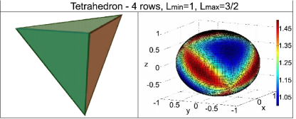
Figure 1: (Color online) Tetrahedron and distributions fidelity loss over the Poincaré-Bloch sphere for the protocol based on tetrahedron geometry. Color bar shows level of average fidelity loss $L$.

Figure 2 presents a cube and an octahedron. These polyhedrons are dual to each other. The maximum losses are equal to 9/8 in both cases.

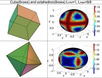
Figure 2: (Color online) Shapes of solids and distributions of average fidelity loss over the Poincaré-Bloch sphere for the protocol based on cube and octahedron geometry. Color bar shows level of average fidelity loss $L$.

Figures 3 and 4 present a dodecahedron and an icosahedron, as well as fullerene and a polyhedron that is dual to the latter: one can clearly see that when the number of projections grows the maximum losses converge to the minimum possible losses. In the limit of infinite number of points on the Bloch sphere we get an optimal protocol for which the precision of reconstruction does not depend on the reconstructed state at all. The price for that would be an infinite growth of the performed measurements, so in a real experiment one should sacrifice the fidelity losses (accuracy) to use a realistic (limited) number of measurements. However, this point is quite common for any quantum tomography protocols exploiting redundant (with respect to dimension of the reconstructed state) number of measurements.

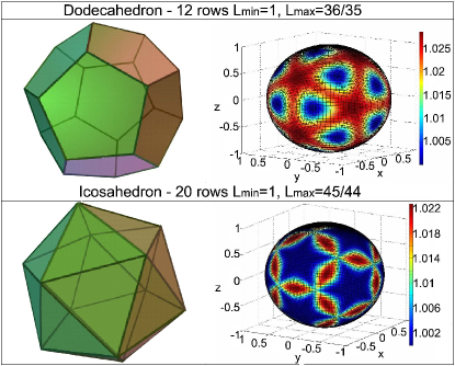
Figure 3: (Color online) Shapes of solids and distributions of average fidelity loss over the Poincaré-Bloch sphere for the protocol based on dodecahedron and icosahedron. Color bar shows level of average fidelity loss $L$.

For the sake of completeness, fullerene and its dual protocols are presented on the last picture, while Table 1 presents the results of numerical experiments for pure quantum states with the number of qubits from 1 to 3. It is worth noting that the algorithm of numerical optimization does not garantee the finding of the global optima. Using the numerical procedure we have only found hypothetical maximum loss values.

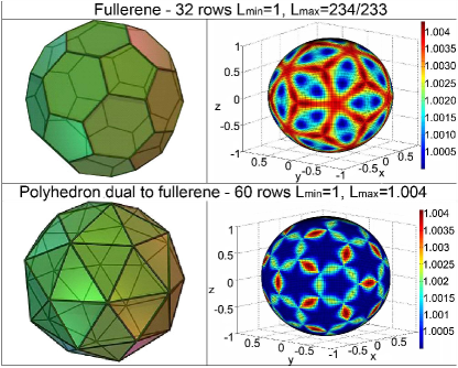
Figure 4: (Color online) Shapes of solids and distributions of average fidelity loss over the Poincaré-Bloch sphere for the protocol based on fullerene and its dual polyhedron. Color bar shows level of average fidelity loss $L$.

The precision of each protocol can be characterized by the following bounds $L_{\text{min}}\leq L\leq L_{\text{max}}$. This inequality defines a rather narrow range, where the precision of quantum state reconstruction is localized definitely.

Numerical calculations demonstrate that the minimum possible losses $L_{\text{min}}$ are defined by the theoretically derived optimal limit $L_{\text{min}}=L_{\text{min}}^{\text{opt}}=s-1$.

By looking to the upper limit $L_{\text{max}}$, shown in the Table 1, as the result of numerical experiments, one can evince that for single-qubit protocols as the number of projections grows the maximum losses converge to the minimum possible losses. In the limit of an infinite number of points on the Bloch sphere one gets an optimal protocol for which the precision of the reconstruction does not depend on the reconstructed state.

However, this is not true for multiqubit protocols. For two-qubit protocols, the maximum possible losses approach the level $L_{\text{max}}\approx 3.38$ while the minimum possible level is equal to $L_{\text{min}}^{\text{opt}}=3$. Similarly for three-qubit states the values are $L_{\text{max}}\approx 7.7$ and $L_{\text{min}}^{\text{opt}}=7$. These results are due to the fact that these protocols are based on projections only onto non-entangled states.

Table 1: Results of numerical experiments that define maximum precision losses $L_{\text{max}}$ for protocols based on the pohyhedron geometry.

	1 qubit	2 qubits	3 qubits
	($s=2$, $L_{\text{min}}=1$)	($s=4$, $L_{\text{min}}=3$)	($s=8$, $L_{\text{min}}=7$)
Tetrahedron ($m=4$)	3/2=1.5	4.442971458	$\approx 10.4$
Cube ($m=6$)	9/8 = 1.125	$\approx 3.5839$	$\approx 8.2$
Octahedron ($m=8$)	9/8=1.125	3.4708(3)	$\approx 7.9$
Dodecahedron ($m=12$)	36/35	$\approx 3.42$	$\approx 7.8$
Icosahedron ($m=20$)	45/44	$\approx 3.39$	$\approx 7.8$
Fullerene ($m=32$)	$\approx 234/233$	$\approx 3.38$	$\approx 7.7$
Polyhedron dual to fullerene ($m=60$)	1.0041037488	$\approx 3.38$	$\approx 7.7$

Here we should stress again that from the theoretical point of view in the multiqubit case the discussed protocols are not the best possible ones because they do not involve projections onto entangled states. In that case the precision will be somewhat smaller than the minimum possible limit. ($L_{\text{max}}\approx 3.38$ compared to $L_{\text{min}}^{\text{opt}}=3$ for two-qubit states and $L_{\text{max}}\approx 7.7$ compared to $L_{\text{min}}^{\text{opt}}=7$ for three-qubit states).

It is also worth noting that, though the protocols based on polyhedrons with small number of faces (tetrahedron, cube) are somewhat less precise, they are much easier in practical implementation.

When considering tomography of mixed states it is worth noting that there is no finite upper limit for precision losses (losses can be infinitely large $L\to\infty$). Such large losses are inherent to mixed states, which are close to pure ones. In fact the number of real parameters that define a mixed state of full rank in Hilbert space of dimension $s$ is equal to $s^{2}-1$, which is significantly greater for large $s$ than for a pure state that takes only $2s-2$ real parameters. In case of a mixed state that has one predominant component, the smaller weight components almost do not affect the statistical data and do not increase the amount of Fisher information for reconstructing the greatly larger number of parameters. Theoretical analysis, numerical and real physical experiments completely prove these statements.

The lower limit for precision losses can be applied to mixed states as well. In this case optimal minimum losses are realized for “white noise states” (uniform density matrix), when all components have equal weights. Then, there is a simple relation between the vector $d$ of dimension $s^{2}-1$, that defines distribution of precision loss, and the vector of singular values of the measurement matrix $B$. Corresponding estimate for $L_{\text{min}}$ for the protocols considered here is given by the following equation:

$$L_{\text{min}}=\left(n\sum_{j}d_{j}\right)_{\text{min}}=\sum_{j}\frac{m^{l}}{4sb_{j}^{2}}=\frac{10^{l}-1}{4}.$$ (41)

This value depends on the number of qubits, but does not depend on the type of polyhedron. It defines the minimum possible losses for the considered protocols that do not use projections on entangled states.

Recall that in the general case for any protocols including those ones that involve projections onto entangled states minimum (optimal) losses are described by:

$$L_{\text{min}}^{\text{opt}}=\frac{\nu^{2}}{4(s-1)}=\frac{(2^{l}+1)^{2}(2^{l}-1)}{4}.$$ (42)

By comparing the Eqs. (41) and (42) one can see that these protocols provide minimum possible (optimal) losses for reconstruction of mixed states of full rank only for single-qubit states. Therefore, for multi-qubit cases protocols that provide minimum possible losses during quantum states reconstruction should necessarily include projections onto entangled states.

Let us consider few examples demonstrating the features of the developed approach. Figure 5 presents the results of numerical experiments testing the universal statistical distribution for fidelity; 200 experiments were conducted with sample size 1 million each.

The measurement protocol is based on tetrahedron. We considered a four-qubit state that represents a mixture of GHZ state and uniform density matrix (white noise):

$$\rho=f\frac{E}{16}+(1-f)|\text{GHZ}\rangle\!\langle\text{GHZ}|,$$ (43)

where $E$ is the unit matrix of size $16\times 16$, $|\text{GHZ}\rangle$ is the state of Greenberger-Horne-Zeilinger: $|\text{GHZ}\rangle=\frac{1}{\sqrt{2}}(|0000\rangle+|1111\rangle)$, and $f$ is the weight of the uniform density matrix (white noise). In our case $f=0.5$ (50%). It is a multiparametric distribution, being the size of the vector of parameters 255. These data (Fig. 5) demonstrate a good agreement between results of a numerical experiment and the theory with high critical significance level (0.65) for $\chi^{2}$ criterion.

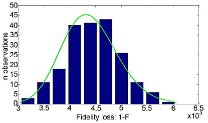
Figure 5: (Color online) The universal statistical fidelity loss distribution for 200 numerical experiments (histogram) compared with the theoretical expectation (solid curve). Sample size of each experiment is 1 million.

Then we consider the dependence of reconstruction precision on the weight of the “white noise” component. The value of fidelity can belong to a wide interval, thus it is convenient to use a new variable $z=-\log(1-F)$. Here and below $\log$ denotes the common logarithm. The new variable $z$ defines the number of nines in numerical representation of fidelity, for example, $z=3$ means that $F=0.999$.

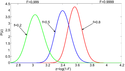
Figure 6: (Color online) Density distribution of the scaled fidelity $z$ for three qubit state with different value of mixture GHZ and “white noise”states. The measurement protocol is based on dodecahedron. Sample size $n$ is equal to one million.

As an another example, Fig. 6 shows distributions calculated by using the new variable for a three-qubit state, which is again a mixture of GHZ state and “white noise” (uniform density matrix). Calculations were performed with a protocol based on dodecahedron. The sample size $n$ is equal to one million as well. It is evident that the higher the white noise weight the higher the precision of reconstruction. It is not difficult to explain this fact in the context of previous discussion. Namely the “white noise” is the best one for mixed state reconstruction.

And finally, Fig. 7 presents the behavior of the reconstruction precision for Bell and GHZ states when the number of qubits grows from two to eight and the sample size is one million. The measurement protocol is based on tetrahedron. It is evident that the precision of reconstruction falls as rapidly as the width of the distribution with increasing the number of qubits.

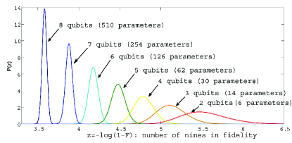
Figure 7: (Color online) Density distribution of the scaled fidelity $z$ for Bell and GHZ states. The measurement protocol is based on tetrahedron. Sample size $n$ is equal to one million.

V Experiment and analysis

For testing the theoretic approach, described in the previous sections, we have prepared a whole family of polarization states for qubits and ququarts. In particular we considered both pure and mixed qubit states and pure, mixed, entangled and separable states of ququarts.

Qubits. The experimental setup for generation and measurement of qubit states is shown in Fig. 8. Setting up the experiment we pursuit the following goals: (1) The setup should allow performing the transition between pure and mixed polarization states of qubits. (2) Three different measurement protocols (R4, K4, B36) should be realized. (3) The setup should allow performing measurements with different sample size (statistics).

To satisfy the first request we used a wide-band light source (incandescence lamp) passing through a monochromator and thick birefringent plates. This provides a variable spectral range around the chosen central wavelength 1.55 ${\mu}$m and a controllable phase delay between basic polarization modes. Therefore, by changing the spectral range of the light (within 1–23 nm) we were able to vary the purity of the output polarization state. A parallel light beam was formed by a $SMF28$ single-mode fiber with $F240FC$-1550 micro-objectives placed at its input and output. A Glan-Thompson prism was used for preparation of the horizontally polarized state $|H\rangle$ serving as initial state for the following transformations. As a result, the original pure state was transformed into a mixed state with a degree of purity, depending on the spectral width of the detected radiation. A smooth transition from pure states to total mixtures was achieved with increasing spectral width of radiation. Since the “measurement part” of the setup had a finite spectral band, the polarization states at different spectral components within this band were integrated, which corresponded to the registration of mixed-polarization state.

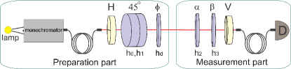
Figure 8: (Color online) Experimental setup for different tomographic reconstructions of qubits with variable degree of mixture. Here H, V are Glan-Thompson prisms, $h_{0}$ is a thick quartz plate, $h_{1}$ is a thick tilt plate, $h_{d}$ is a driving phase plate, $h_{2,3}$ are tomographic phase plates, and D is a detector.

For the preparation of pure polarization states of qubits we selected a spectral range about 1 nm. The initial state $|H\rangle$ passed through a phase plate $h_{d}$ (436 $\mu$m) oriented at $0^{\circ},45^{\circ}$. So the states under consideration had the following form respectively:

$$|\Psi_{1}\rangle=|H\rangle,|\Psi_{2}\rangle=0.345|H\rangle-0.939i|V\rangle.$$ (44)

The second requirement is achieved with a standard quantum tomography method that used two achromatic quartz plates $h_{2}$=441 $\mu$m, $h_{3}$=313 $\mu$m served for reconstruction of polarization states. These plates were oriented at particular angles $\alpha,\beta$ (with respect to the vertical axis), so light passing through the plates and following vertical polarizer was projected onto the necessary set of states required by protocols J4 and R4. In the first protocol J4, suggested in Kwiat , projective measurements upon some components of Stokes vector were performed: $|H\rangle,|V\rangle,|45^{\circ}\rangle=\frac{1}{\sqrt{2}}(|H\rangle+|V\rangle),|R\rangle=\frac{1}{\sqrt{2}}(|H\rangle+i|V\rangle)$. Basically the projective measurements can be chosen arbitrarily, in particular if the measured qubits were projected on the states possessing tetrahedral symmetry then the protocol transforms to R4. There are several works showing that due to the high symmetry such protocol provides a better quality of reconstruction Rehacek ; Ling ; Lingtwo . Another protocol B9 exploits a single plate and fixed polarizer. The corresponding measurements have been performed for each of the nine orientations of the plate with a step of $20^{\circ}$. We have chosen the “optimal” thickness of the plate $h_{3}$=313 $\mu$m and achieved the better condition number ($K=2.7$) for reconstruction of mixed states. Also for testing theoretical predictions with this protocol we used other plates $h_{3}$=824 $\mu$m and $h_{3}$=358 $\mu$m and corresponding condition numbers were $K_{824}=14.9$ and $K_{358}=183.9$.

The third requirement was satisfied by using a single-photon detector based on GaAs-based avalanche photodiode with a pigtailed input and an internal gate shaper Molotkoff . The total number of registered events was varied by changing the gate rate at a fixed gate width (about 10 ns). This simply follows from the fact that the fixed photon flux comes continuously and increasing (decreasing) the gate width just increases (decreases) the probability to register a photon.

The goal of our first experiment was the optimization of a quantum tomography protocol for polarization qubits. As an example we selected protocol B9 implemented by means of a single phase plate and a fixed polarizer. Note that the projection in the protocol B9 is performed onto non-fixed states, in contrast to the protocols J4, K4, and depends on the parameters of the plate, that is, on its optical thickness, $\delta=\pi h\Delta n/\lambda$, and the orientation angle $\beta$, where $\Delta n$ is the birefringence of the plate material at a given wavelength $\lambda$ and $h$ is its geometric thickness. It is worth to mention that the parameters of this protocol can be chosen by doing the experiment, depending on available resources: in some sense this choice can be done in an optimal way, but using the plate with optimal condition number. Figure 9 shows the calculated condition numbers $K$ and maximum losses $L$ on the Poincaré-Bloch sphere as functions of the optical thickness of the phase plate for the B9 protocol. The dependencies are periodic with a period of $\pi$. Poor conditionality occurs at $\delta=0,\frac{\pi}{2},\pi$. Both quantities $K$ and $L$ tend to infinity at these particular points. For this protocol the best (lowest) achievable parameter $K$ takes the value 1.85. For example, to reach such a value one might choose plates with optical thickness $\delta=0.356\pi$ or $\delta=0.644\pi$. The corresponding condition numbers for protocols J4, R4 are $K_{\text{J4}}\approx 3.23$ $K_{\text{R4}}=\sqrt{3}\approx 1.73$. Particularly for our experiment we have chosen a set of following three plates: $h_{3}$=313 $\mu$m (optimal), $h_{3}$=824 $\mu$m (medium), $h_{3}$=358 $\mu$m (nonoptimal) with condition numbers $K=2.7$, $K=14.9$ and $K=183.9$. The optimal value of maximum losses $L_{\text{opt}}=1.47$ occurs at the points $\delta=0.391\pi,0.609\pi$. The corresponding losses are somewhat lower than those for the R4 protocol ($L=1.5$), and essentially lower than those for the J4 protocol ($L=4.52$). Note that these curves on Fig. 9 are similar in form, but their minima correspond to slightly different values of $\delta$. However, the singular values of $K$ and $L$ correspond to the same $\delta$ value. Thus, both criteria allow separating the regions of the protocol parameters for which the results would be unsatisfactory. Unfortunately, for a large dimension of the Hilbert space for reconstructed states, the scanning of $L$ values is a complicated computational problem. For this reason, to optimize such protocols, we suggest to use the parameter $K$.

Figure 10 demonstrates the crucial difference between the optimal and nonoptimal approach for the example of considered protocol B9. Here the optimal protocol [Figs. 10(a) and 10(b)] corresponds to the plate with thickness $h$=293.8 $\mu$m and condition number $K=2.2548$. This protocol provides the minimum of maximally possible losses (minimax). The nonoptimal protocol [Figs. 10(c) and 10(d)] corresponds to the plate with thickness $h$=358 $\mu$m and condition number $K=183.9$. The sample size is $10^{4}$. Figures 10(a) and 10(b), which correspond to the optimal protocol, describe the case of guaranteed number of nines in Fidelity being not less than $z_{\text{min}}=3.83$ (so that the mean fidelity (22) for all states on Bloch sphere can not be lower). At the same time, Figs. 10(c) and 10(d), which correspond to the nonoptimal protocol, stand for a very low level of fidelity ($z_{\text{min}}=0.065$), which means that almost none of the states on Bloch sphere can be reconstructed using the protocol. Figures 10(b) and 10(d) are different from Figs. 10(a) and 10(c) by the step of the plate orientation [20 degrees for Fig.10(a) and 10(c) and 1 degree for Figs. 10(b) and 10(d), respectively], so that the number of rows in the protocol grows from 9 to 180. We see that Fig. 10(b) defines a more symmetric distribution of precision compared to Fig. 10(a), even though the range of values [$z_{\text{min}}$, $z_{\text{max}}$] barely changes. A comparison of Fig. 10(c) with Fig. 10(d) shows that in the nonoptimal case increasing the number of projections little affects the distribution of Fidelity on Bloch sphere.

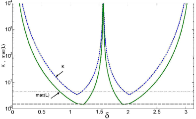
Figure 9: (Color online) Calculated condition numbers K and maximum losses $\max(L)$ on the Poincaré-Bloch sphere versus the optical thickness $\delta$ of a phase plate for the B9 protocol. The dashed and dash-dotted lines are for the R4 and J4 protocols, respectively.

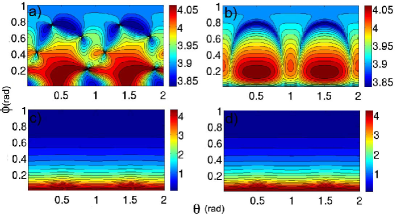
Figure 10: (Color online) Difference between the (a) and (b) optimal and (c) and (d) nonoptimal approach for protocol B9. (a) and (c) and (b) and (d) correspond to $20^{\circ}$ and $1^{\circ}$ steps of the plate orientation, respectively.

For protocol B9 the statistical reconstruction of the prepared states (44) has been performed at given sample sizes. One of the considered states $|\Psi_{1}\rangle$ belongs to an area of small losses for all three plates, and the second state $|\Psi_{2}\rangle$ was changed out of this area. As an example, we present Fig. 11 that shows the calculated widths of fidelity distributions at $1\%$ and $99\%$ quantiles as well as the experimentally reconstructed values for the states (44). Two polarization states (44) were measured and reconstructed using three phase plates chosen above. Experiments were performed with different sample sizes; that is, the total number of the pulses coming from single-photon detector in a fixed time was varied and served as a parameter of the problem.

Figure 11: (Color online) Reconstruction of pure qubit states by protocol B9 at different thicknesses of the plate. Vertical bars show 1% and 99% quantiles for fidelity distributions. Dotted lines connecting lower bar ends point out critical significant levels.

The approach described above provides the ideal accuracy level for quantum state reconstruction. It means that the fluctuations of the estimated quantum states cannot lead to uncertainties smaller than this limit. The presence of instrumental errors and uncertainties makes this level to be exceeded. Indeed, Fig. 11 shows that, above some sample size, the experimental value of fidelity falls out the theoretical uncertainty boundary shown as dotted lines (corresponding to $1\%$ significance level which characterizes a given protocol). This happens since instrumental uncertainties prevail over the statistical ones and indicates that either state preparation stage or measurement procedure were not performed accurately enough. It is clearly seen that both theoretical distributions and experimental points for protocol with nonoptimal choice of plates strongly depend on an initial state. The quality of reconstruction (fidelity) is varied in the range 0.6030–0.9999 for both reconstructed states for the protocol with the plate $h_{3}$=358 $\mu$m (nonoptimal) and in the range 0.9950–0.9997 for the plate $h_{3}$=313 $\mu$m (optimal). It means that if the set of initial states is known (as it happens in quantum process tomography) one can choose the parameters of the protocol that are not optimal for an arbitrary state, but provide the highest accuracy for the selected set of states. In both cases, when the input states are unknown, like in quantum state tomography, it is better to use optimal choice of the plates with minimal condition number, that will ensure high accuracy of the reconstruction of arbitrary states.

Mixed States: modeling and experiment. The goal of the second experiment with qubits was the generalization of the developed approach to the family of mixed states of polarization qubits general-appr . As an example we have tested three protocols again, namely J4, R4, and B36. The protocol B36 has been considered at optimal parameters (phase plate $h_{3}$=313 $\mu$m). This protocol is similar to the one described above (B9), but measurements were performed at 36 consistent orientations of the phase plate ($0^{\circ}$–$360^{\circ}$, step $10^{\circ}$) instead of 9.

As we have pointed out before, the condition numbers $K$ for R4 and J4 protocols take the following values: $K_{\text{R4}}=\sqrt{3}\approx 1.73$, $K_{\text{J4}}\approx 3.23$ while for B36 it becomes $K_{\text{B36}}\approx 2.7$. Thus, we expect that the symmetrical protocol $R4$ provides with better state reconstruction quality. We have checked this statement with numerical simulations of each protocol applied to qubit states with various degree of mixture depending on the sample size.

For the preparation of mixed states we started from a pure state $|\Psi_{1}\rangle=|H\rangle$ which passed through one or two thick birefringent plates, oriented at $45^{\circ}$, where partial decoherence between vertical and horizontal basic polarizations took place. For that purpose we used a quartz plate with a thickness of $h_{0}$=10 mm and additional tiff plate with a thickness of $h_{1}$=4 mm. Changing the width of the spectrum it is possible to pass from completely coherent (pure) case to a very narrow spectral line to a completely incoherent (i.e. mixed in polarization), when the difference between the optical lengths for two orthogonal polarizations exceeds the coherence length of the radiation under consideration:

$$h_{0}(n_{\bot}-n_{\|})_{\text{quartz}}+h_{1}(n_{\bot}-n_{\|})_{\text{tiff}})\gg l_{coh},$$ (45)

where

$$l_{coh}\approx\frac{\lambda^{2}}{\triangle\lambda}\approx 100~{}\mu\text{m}.$$

Thus, at the output of plates $h_{0},h_{1}$ components with orthogonal polarizations evolve with a random phase, which leads to a mixed state.

For determining the accuracy of quantum tomography and fidelity, we need to calculate the density matrix of a prepared mixed state. For this purpose we divide the frequency spectrum of the radiation in small parts and represent the polarization state of a qubit as a superposition of states corresponding to different frequencies in the spectrum:

$$\begin{array}[]{cc}|\Psi\rangle=\sum_{k}a_{k}|\Phi(\omega_{k})\rangle,\\ |\Phi(\omega_{k})\rangle=c_{1}(\omega_{k})|H\rangle+c_{2}(\omega_{k})|V\rangle,\end{array}$$ (46)

where amplitudes $a_{k}$ are defined by the spectrum shape. The density matrix of the state before transformation (46) has the form:

$$\rho^{\text{in}}=|\Psi\rangle\!\langle\Psi|=\sum_{k,j}a_{k}a_{j}^{\ast}|\Phi(\omega_{k})\rangle\!\langle\Phi(\omega_{j})|$$ (47)

The next step of modeling includes the calculation of phase plates action on the qubit state. The unitary transformation on state (47) is given by matrix

$$G(\omega_{k})=\left(\begin{array}[]{cc}t_{k}&r_{k}\\ -r_{k}^{\ast}&t_{k}^{\ast}\\ \end{array}\right)$$ (48)

where

$$\begin{array}[]{cc}t_{k}=\cos\delta_{k}+i\sin\delta_{k}\cos 2\alpha,\\ \quad r_{k}=i\sin\delta_{k}\sin 2\alpha,\delta_{k}={\pi(n_{o}^{k}-n_{e}^{k})h/\lambda_{k}}.\end{array}$$ (49)

Here $t_{k}$ and $r_{k}$ are the amplitude transmission and reflection coefficients of the wave plate at fixed frequency, $\delta_{k}$ is its optical thickness, $h$ is the geometrical thickness, $\alpha$ is the orientation angle between the optical axis of the phase plate and vertical direction. The measurement part of the experimental setup does not distinguish frequency modes, so the theoretical polarization mixed state will be described by a reduced density matrix:

$$\rho=\sum_{k}|a_{k}|^{2}G(\omega_{k})|\Phi(\omega_{k})\rangle\!\langle\Phi(\omega_{k})|G^{+}(\omega_{k}).$$ (50)

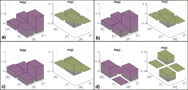
Figure 12: (Color online) Theoretical distribution of the real and imaginary parts of the density matrix for states with varying degrees of purity. The spectral widths of the spectrum are (a) 1.6 nm, (b) 7 nm, (c) 13 nm. Distribution (d), for 22 nm, corresponds almost to a completely mixed state.

The corresponding density matrixes are obtained by integrating formula (50) with the distribution of weights $|a_{k}|^{2}$ as a function $\hbox{sinc}^{2}(x)$. Figure 12 shows the graphical representations of the real and imaginary parts of the theoretical qubit density matrices at different widths of the spectrum: 1.6 nm, 7 nm, 13 nm, 22 nm. When increasing the width of the spectrum the non-diagonal components, responsible for the correlation, decay and the state becomes completely mixed.

In the experiment we have prepared four polarization states of qubit with following degrees of mixture: 3% (1.6 nm), 30% (7 nm), 66% (13 nm), 100% (22 nm), where the state purity is analyzed by calculating the state entropy defined as $S=-\sum_{n=1}^{2}\lambda_{n}\log_{2}\lambda_{n}$, $\lambda_{n}$ being the eigenvalues of the density matrix $\rho$. For each protocol various measurements at different sample sizes were performed. The results are shown in Fig. 13.

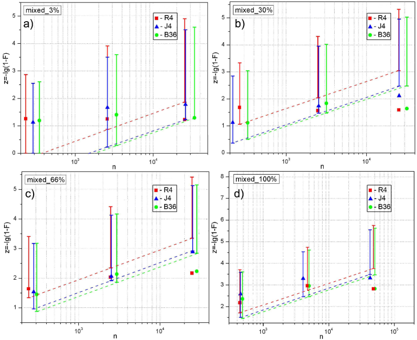
Figure 13: (Color online)Reconstruction of qubits states with various degree of mixture. Vertical bars show 1% and 99% quantiles for fidelity distributions. Dotted lines connecting lower bar ends point out critical significant levels. (a) mixed 3%, (b) mixed 30%, (c) mixed 66%, and (d) mixed 100%.

Figure 13 presents the theoretical distributions of fidelity at 1% and 99% quantiles for each considered protocol. Experimental values are indicated by points. The dashed lines connecting the 1% quantiles show a theoretical lower boundary of the fidelity distribution and depend on the type of protocol: the lower line, the greater condition number and the function of losses. Fig. 13 demonstrates that for a small sample size statistical uncertainties dominate over the instrumental ones. Starting from sample size about $(2-3)\times 10^{3}$ the experimental points fall out the theoretical uncertainty boundary and the protocol achieves a coherent sample size. This means that instrumental uncertainties (the accuracy of setting angles, thicknesses of phase plates, etc.) prevail over the level of statistical errors. From this point a further increase of sample size does not improve the quality of the reconstruction of the quantum state. However, a comparison of experimental results with the theoretical distribution serves as effective method for setup adjusting, stability of the preparation/measurement systems, etc.

Furthermore, from Fig. 13 one can evince that the accuracy of the reconstruction increases with the degree of mixture: for the states close to a pure ones (3% mixture) the fidelity achieves an average value 0.93–0.94, while the best accuracy is achieved for totaly mixed state corresponding to the center of the Bloch sphere, $F>0.99$. The theoretical estimates are consistent with both numerical and real experiments.

Ququarts: pure and mixed states, preparation and measurement. For a further verification of our approach we prepared also a family of quqarts biphoton polarization states se , which can be easily converted into either entangled (in polarization) or factorized states, both pure and mixed.

$$\begin{array}[]{cc}\rho=(1-p)|\Psi_{\text{pure}}\rangle\!\langle\Psi_{\text{pure}}|+\frac{p}{2}(|H_{1}H_{2}\rangle\!\langle H_{1}H_{2}|\\ +|V_{1}V_{2}\rangle\!\langle V_{1}V_{2}|),\end{array}$$ (51)

where

$$|\Psi_{\text{pure}}\rangle=c_{1}|H_{1}H_{2}\rangle+c_{2}e^{i\varphi}|V_{1}V_{2}\rangle$$ (52)

with real amplitudes $c_{1}$ and $c_{2}$ and relative phase shift $\varphi$. The coefficient $p$ defines the degree of mixture.

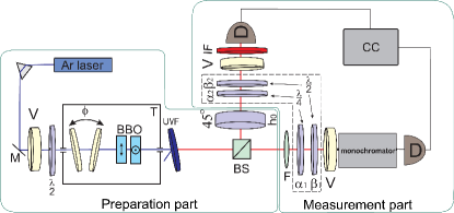
Figure 14: (Color online) Experimental setup for different tomographic reconstructions of photon pairs with variable polarization entanglement and degree of mixture. Ar laser: argon laser with wavelength 351 nm, M: mirror, V: vertical oriented Glan-Thompson prism, BBO: nonlinear Barium Borate crystals, UVF: ultraviolet filter, $\lambda_{p}/2$, $\lambda_{p}/4$: half-wave, quarter-wave plates, L: lens with focus 20 cm, BS: beamsplitter, IF: interfilter, D: avalanche photodetectors, CC: coincidence circuit.

The set-up is schematically depicted in Fig. 14. For generation of pure biphoton-based polarization ququarts ($p=0$) we used a set of two orthogonally oriented type-I BBO crystals (1 mm), cut for collinear, frequency non-degenerate phase-matching around the central wavelength of 702 nm. The crystals were pumped by a 600 mW cw-argon laser operating at 351 nm. The Glan-Thompson prism (V) at vertical polarization and the half-wave plate ($\lambda_{p}/2$) placed in front of crystals allowed rotating the polarization of the pump by the angle $\phi$, which controlled the real amplitudes $c_{1}$ and $c_{2}$ in (52). A set of quartz plates $QP$ introduced the relative phase shift $\varphi$ between the horizontal and the vertical components of the UV pump. If $\phi=0$ we prepared the state $|\Psi\rangle=|V_{1}V_{2}\rangle$, if $\phi=22.5^{\circ}$ and $\varphi=3\pi/2$ then the state transformed to $|\Psi\rangle=\frac{1}{\sqrt{2}}\left(|H_{1}H_{2}\rangle-|V_{1}V_{2}\rangle\right)\equiv|\Phi^{-}\rangle$. To maintain stable phase-matching conditions, BBO crystals and QP were placed in a closed box heated at fixed temperature. The lens $L$ coupled SPDC light into the monochromator M (with 4 nm resolution), set to transmit “idler” photons at 710 nm. The conjugate “signal” wavelength 694 nm was selected automatically by means of the coincidence scheme.

In order to prepare a mixed state it is necessary to introduce quantum distinguishability among the biphoton ququart basis states in a controllable manner. For the preparation of states with various degree of mixture the double-crystal scheme was complemented by a quartz plate with thickness $h_{0}$, which was putted in the reflected arm of Brown-Twiss scheme. A thick quartz plate with vertically oriented optical axis introduced a delay between vertically and horizontally polarized photons that led to their temporal distinguishability, and hence, to the emergence of a mixture. Changing the width of the frequency spectrum, which, in our case, was determined by the width of the monochromator slit, or the plate thickness it was possible to change the visibility of polarization interference. Our goal was the preparation and reconstruction (by several protocol, including non-optimal ones) of a set of states with different degree of entanglement and set of mixed two-qubit states.

The reconstruction part for the ququart is shown in Fig. 14. First, the photon pair that forms the biphoton-ququart was split into two spatial modes by using a beam splitter BS. A photon in each arm, then, underwent a polarization state transformation with the use of a couple of zero-order wave plates ($\lambda/2$,$\lambda/4$) for protocols. Two Si-APD’s linked to a coincidence scheme with 1.5 ns time window were used as single photon detectors. Registering the coincidence rate for different projections, that were realized by the half- and quarter-plates and a fixed analyzer, was possible to reconstruct the polarization state of ququarts by protocols R16, J16, described above. This scheme also allowed reconstructing any arbitrary polarization ququart state by protocol B144. For the reconstruction of ququarts pure states by protocol B144 we used two retardation plates Wp1, Wp2 placed before beam splitter and deleted half-wave and quarter-wave plates. Unfortunately, this method can not be applied for the reconstruction of mixed states of ququarts. This is due to the feature of preparation for mixed states: all projection measurements must be done after state preparation that is violated for such configuration of the tomography protocol. To solve this problem, we have used an equivalent scheme. In each arm we have established a couple of identical plates Wp1, Wp2 instead of half-wave, quarter-wave plates and rotated them synchronously. This scheme is completely equivalent to the standard protocol B144, but slightly more complicated in realization. By analogy to protocols B9 and B36 with single retardant plate we can choose the optimal parameters for protocol B144.

Let us analyze how the choice of plates thicknesses affects the quality of state reconstruction.

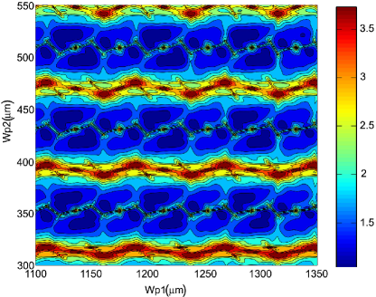
Figure 15: (Color online) Dependence of $\log(K)$ on plates thicknesses for protocol B144.

Figure 15 presents the calculated condition number $K$ in common logarithmic scale for the set of thicknesses of the first and second quartz retardant plates. Specifically the first plate Wp1 was varied within the limits from 1.100 to 1.350 mm with a step 0.001 mm and a second plate, Wp2, was varied within the limits from 0.300 to 0.550 mm with the same step. Here the thicknesses of the first and second quarts retardant plates are shown along the axis $x,y$, correspondingly. Blue color indicates areas with low value of condition number $K$, while the red one indicates areas with high value of $K$. It is obvious, that the arbitrary choice of plates most likely will be wrong from the point of view of completeness of matrix $B$ and protocol optimality. In other words this figure serves as some sort of a “navigation map” for the measurement protocol. So to achieve good quality of the measurement one should select the plates thicknesses in blue areas and avoid red areas. For the present protocol the minimum achievable $K$ is 11.35. For example, to reach such a value one can choose plates with thickness Wp1=1.207 mm and Wp2=0.520 mm. In our specific experimental configuration we have selected the plates Wp1=1.303 mm and Wp2=0.440 mm. Such thicknesses of the plates for the protocol B144 were chosen to show the difference in the quality of reconstruction.

For all three protocols used in the experiment we have calculated the condition numbers $K$, which assume the following values: $K_{\text{R16}}=3$, $K_{\text{J16}}\approx 10$, $K_{\text{B144}}\approx 60$. Thus, we expect that the symmetrical protocol R16 provides with better state reconstruction quality Burgh and the protocol B144 provides the worst one. We have checked this statement with numerical simulations of each protocol applied to different two-qubit states depending on the sample size.

As an example, let us consider the numerical reconstruction of the Bell state $|\Phi^{-}\rangle=\frac{1}{\sqrt{2}}\left(|H_{1}H_{2}\rangle-|V_{1}V_{2}\rangle\right)$. Figure 16 shows average fidelities, calculated according to (21) as functions of a sample size for each protocol. It turns out that the difference between curves disappears at sufficiently large sample size ($10^{5}$)instrumental , but for the same quality of state reconstruction the correct choice of protocol allows using a smaller set of statistical data, i.e. finally reduces total acquisition time. Figure 16 shows that protocols are ranged in accuracy as following: R16, J16, and B144 in complete agreement with the range given by condition number $K$. Figure 17 presents accuracy distributions calculated according to (21) for the sample size $3\times 10^{3}$.

It is clearly seen that the density distribution for the R16 protocol is narrower than the one for J16 and B144 and localizes in the region of lower losses or higher fidelities. The distribution for B144 is broader and lower in comparison with R16 and J16. Obviously, the narrower distribution of fidelity indicates a better reconstruction quality in the sense that the reconstruction procedure returns a better-defined state. Thus, Figure 17 confirms our expectation based on estimation of condition number $K$: R16 achieves the best results.

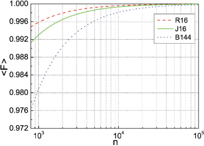
Figure 16: (Color online) Dependence of the average fidelity on number of registered events forming the sample for Bell state reconstructed by protocols J16, K16 and B144.

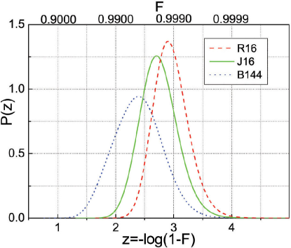
Figure 17: (Color online) Density distribution of the scaled fidelity $z$ (lower abscissa) at $n=3\times 10^{3}$ for Bell state reconstructed by protocols J16, K16 and B144. Upper abscissa presents regular fidelity.

Let us consider now the experimental results. As an example, Fig. 18 shows both experimental points and theoretical distributions for the set of pure ququart states with various degree of entanglement: $C_{\varphi_{1}}=0$, $C_{\varphi_{2}}=0.66$, $C_{\varphi_{3}}=0.83$, $C_{\varphi_{4}}=1$ correspondingly. Here $C_{\varphi_{i}}$ is quantity concurrence, which is defined as $C=2|c_{1}c_{4}-c_{2}c_{3}|$ and $C=0$ for a separable state and $C=1$ for a maximally entangled state.

Figure 19 presents experimental points and theoretical distribution for the set of mixed ququart states with various degree of mixture: $p=1,~{}0.3,~{}0.7$ ($p=1$ corresponds to totaly mixed state, $p=0.3$ means that state contains 30% of mixture.)

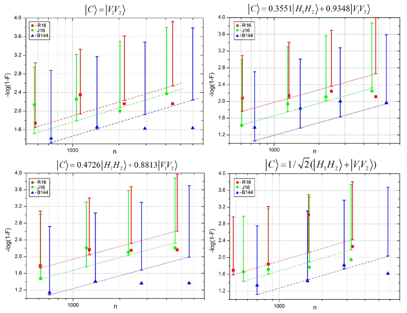
Figure 18: (Color online) Reconstruction of ququart states with various degree of entanglement. Vertical bars show 1% and 99% quantiles for fidelity distributions. Dotted lines connecting lower bar ends point out critical significant levels.

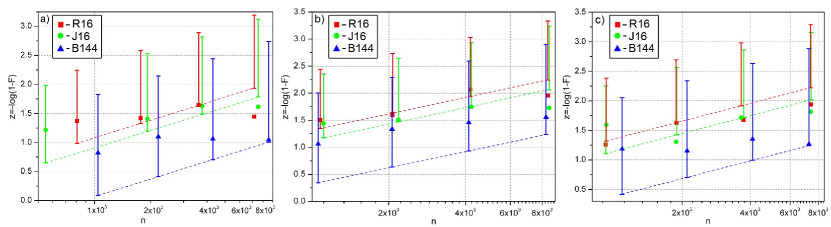
Figure 19: (Color online) Reconstruction of ququart states with various degree of mixture. Vertical bars show 1% and 99% quantiles for fidelity distributions. Dotted lines connecting lower bar ends point out critical significant levels. (a) $p=0.3$, (b) $p=0.7$, and (c) $p=1$.

On both figures the agreement between the experimental results and a priori calculated expectations is noteworthy.

Figure 19 shows that the accuracy of reconstruction increases with the degree of mixture. However from a statistical point of view there is a problem. A small weight of the mixed states, adding to the original pure state, leads to a small change in the statistical data while the number of parameters for ququart state increases from 6 to 15. As a result the amount of new information that arises in quantum measurements is not sufficient to achieve an adequate estimation of all the parameters.

VI Discussion

Many remarkable works in quantum state tomography developed different theoretical approaches. In the present section we shall briefly discuss the features and advantages of our approach in this framework.

One of the main issues in quantum tomography is the choice of adequate parameterization for quantum states. Bloch sphere representation is one option. In this representation density matrix $\rho$ is defined in Hilbert space of dimension $s$ by the following equation Kwiat ; Nunn ; Paris-Reh

$$\rho=\frac{1}{s}E+\nu_{j}\sigma_{j},$$ (53)

where $E$ is the $s\times s$ identity matrix, $\nu_{j}$ is a vector in real Euclid space of size $s^{2}-1$, and $j$ changes from 1 to $s^{2}-1$. Respective Hermitian basis matrices $\sigma_{j}$ meet the following conditions:

$$\hbox{tr}(\sigma_{j})=0,\,\,\,\,\,\hbox{tr}(\sigma_{j}\sigma_{k})=\delta_{jk}.$$ (54)

Note, that for single-qubit states when $s=2$, matrices $\sigma_{j}$ coincide with ordinary Pauli matrices (multiplied by $\frac{1}{\sqrt{2}}$). The radius of 3D Bloch sphere in this representation is also equal to $\frac{1}{\sqrt{2}}$.

One may easily calculate Bloch vectors $\nu_{j}$ from the known density matrix $\rho$:

$$\nu_{j}=\hbox{tr}(\rho\sigma_{j}).$$ (55)

However, Bloch parameterization has a significant drawback. For every real vector $\nu$ Eq. (53) guarantees that the density matrix $\rho$ is Hermitian, but does not guarantee that it is positively defined. As a result, we can obtain a non-physical density matrix using Eq. (53). Separation of admissible density matrices from those that can not physically exist is a non-trivial task for all dimensions higher than two. In particular, for $s>2$ Bloch representation is practically useless for description of matrices of non-full rank, for which the number of degrees of freedom of quantum state (36) is less than dimension of Bloch vector $s^{2}-1$. This drawback of Bloch parameterization complicates the use of Fisher information matrix and calculation of statistical estimates’ precision in general.

An adequate and convenient procedure of parameterization is important for numerical procedures of calculating density matrix from experimental data because for every iteration the approximate solution must lie in the range of physical density matrices only. For instance, such issues may arise for problems of estimation of quantum state by maximum likelihood method.

The problem of estimating a density matrix by maximum likelihood method was considered in Hradil ; T ; Zambra ; Allevi . The respective likelihood equation has the following form Hradil ; Paris-Reh ; Hradil-Summ :

$$R\rho=\rho,$$ (56)

where $R$ is some operator.

The iteration procedure from $j$th to $j+1$th step for this equation has the following form: $\rho^{j+1}=R\rho^{j}$. Such procedure, however, does not even provide Hermitian property for density matrix.

Another procedure that is widely used Paris-Reh $\rho^{j+1}=\frac{1}{2}(R\rho^{j}+\rho^{j}R)$ provides the Hermitian property but does not guarantee positive definiteness in general. Fortunately there are known robust, well-converging procedures providing with both Hermiticity and positive definiteness simultaneously Lv .

In this paper we consider a natural approach for quantum theory that is based on representing the quantum state as a mix of pure states Bogdanov ; Bogdanovtwo ; JETPLBogd . Consider transformation of the density matrix to diagonal form.

$$\rho=UDU^{\dagger}.$$ (57)

Here $U$ is an unitary matrix (its columns define eigenvectors of density matrix), $D$- is a diagonal non-negative matrix (its diagonal is formed by eigenvalues of density matrix that we shall put in decreasing order). Let the rank of density matrix be $r$ ($1\leq r\leq s$). We shall eliminate all non-zero rows and columns of matrix $D$ and shall leave only the first $r$ columns in matrix $U$. Then the density matrix could be represented in the following compact form.

$$\rho=LL^{\dagger},$$ (58)

where $L=UD^{\frac{1}{2}}$.

Here $L$ is a complex matrix of dimension $s\times r$ that defines the actual parameterization of density matrix. It represents a purified state vector (probability amplitudes). For representation as a column vector, one should simply place the second column under the first one and so on. Note that the purified state is defined ambiguously, because the density matrix does not change during transformation

$$L\rightarrow L^{\prime}=LV,$$ (59)

where $V$- is an arbitrary unitary matrix of size $r\times r$.

It is crucial that the ambiguity (59) does not affect the procedure of statistical reconstruction of density matrix, because all possible purified state vectors define the same density matrix.

We can choose the unitary transformation $V$ such that in matrix $L^{\prime}$ all elements on the principal diagonal will have real strictly positive values, while elements higher the principal diagonal shall be equal to zero.

For a density matrix of full rank, such matrix $L^{\prime}$ shall form a lower triangular matrix. In mathematics such decomposition is usually called Cholesky decomposition. Representation of density matrix in such form was originally studied in Banaszektwo . Note that from the point of view of physics, Cholesky representation is just one of the possible ways of recording a purified quantum state.

A purified state vector represents the most simple and most natural in view of physics form of parameterization of density matrix. It is important that parameterization based on purification of quantum state radically simplifies the theory of statistical estimates.

For example, the precision of estimates by maximum likelihood method is defined by matrix of full information that is analogous to Fishers information matrix in relation to estimation of quantum state vector Bogdanov ; Bogdanovtwo ; JETPLBogd .

The matrix of full information is defined by the following equation:

$$H=2\sum_{j}\frac{t_{j}(\Lambda_{j}c)(\Lambda_{j}c)^{+}}{\lambda_{j}}.$$ (60)

The object is defined in real Euclidian space of dimension $2rs$. To obtain state vector $c$ in this representation, one should place the imaginary part of purified state vector under its real part. Intensity matrices $\Lambda_{j}$ represent expansion of matrices (6) to the considered Euclid space. The sum in Eq. (60) is taken for all measurement protocol rows. Matrix $H$ becomes a real symmetric matrix of dimension $2rs\times 2rs$.

If the quantum measurement protocol is complete, then for the information matrix $H$ $\nu_{H}=(2s-r)r$ out of $2rs$ eigenvalues are strictly positive, while the other $r^{2}$ are equal to zero. One may formulate a universal statistical distribution (21) based on information matrix $H$ that will describe precision of statistical reconstruction of quantum states.

Eigenvectors of matrix $H$ corresponding to non-zero eigenvalues define directions of fluctuations of a quantum state and its norm, while eigenvectors that correspond to zero eigenvalues define directions of insignificant fluctuations that are due to the ambiguity (59) in definition of the purified state vector.

While information matrix $H$ defines detailed characteristics of precision of reconstruction of an arbitrary quantum state, the measurement matrix $B$ (9) defines the quality of the protocol as a whole. The condition number $K$ separates complete and well defined quantum measurement protocols from incomplete and ill-defined ones.

The approach developed above is based on analysis of completeness, adequacy and precision of quantum measurements and it could be applied to analysis of quality and efficiency of arbitrary protocols of quantum measurements.

As a simple example, let us consider a single-qubit protocol proposed in works Nunn ; Kosut_Walm (see Fig. 1 in Nunn and Fig. 3 in Kosut_Walm ). The considered approach is an optimized measurement of state

$$c=\frac{1}{\sqrt{2}}\left(\begin{array}[]{c}1\\ 1\end{array}\right).$$

Measurements are conducted by means of a set of half- and quarter- wave plates that lead to projections to the following basis states

$$\psi_{1}=\frac{1}{\sqrt{2}}\left(\begin{array}[]{c}\sin(2h)+i\sin(2(h-q))\\ \cos(2h)-i\cos(2(h-q))\end{array}\right).$$

$$\psi_{2}=\frac{1}{\sqrt{2}}\left(\begin{array}[]{c}\cos(2h)+i\cos(2(h-q))\\ -\sin(2h)+i\sin(2(h-q))\end{array}\right).$$

where $h$ and $q$ are orientation angles for half-wave and quarter-wave plates respectively. This measurement defines two strings of instrumental matrix $X$. The authors of the protocol proposed a set of four measurements of such type (8 rows in total). Measurements are defined by the following orientation angles for the plates: $h_{1}=0^{\circ}$, $q_{1}=0^{\circ}$; $h_{2}=20^{\circ}$, $q_{2}=45^{\circ}$; $h_{3}=25^{\circ}$, $q_{3}=45^{\circ}$; $h_{4}=45^{\circ}$, $q_{4}=0^{\circ}$.

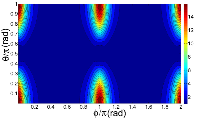
Figure 20: (Color online) Analysis of precision losses for protocol proposed in Kosut_Walm ; Nunn .

A complete analysis of precision losses (34) during reconstruction of single-qubit pure quantum states using the protocol is given in Fig. 20 (little precision loss states are marked blue, large precision losses a marked brown). We see that for the state

$$c=\frac{1}{\sqrt{2}}\left(\begin{array}[]{c}1\\ 1\end{array}\right)$$

the protocol is indeed the optimal one because the losses are at minimum $L_{\text{min}}=1$. However for a number of other states the protocol is rather not optimal (maximum losses are quite large $L_{\text{max}}\approx 16.84$). For instance, the protocol considered here has much less precision than those studied in section VI which are based on symmetries of cube and octahedron and which also have few rows (6 and 8 respectively), but provide much lower precision losses in narrow range from $L_{\text{min}}=1$ to $L_{\text{max}}=9/8$.

Note that the condition number $K$ for the protocol is approximately $4.07$ times higher than for protocols based on regular polyhedrons, which also certifies its lower quality.

VII Conclusions

In this paper, we proposed a methodology to assess the quality and efficiency of quantum measurement protocols. It was shown that the proposed approach, based on the analysis of completeness, adequacy and accuracy, can be successfully applied to arbitrary quantum states and measurement protocols. Analysis of the completeness of the protocol allows to answer the question: Is the set of operators considered sufficient to assess an arbitrary pure or mixed quantum state? The operational criterion of the protocols’ quality follows from the analysis of completeness. The criterion is based on the condition number of the measurements matrix $K$. An analysis of the adequacy allows one to answer the question about the correspondence between the statistical experimental data and the quantum-mechanical mathematical model. The analysis of the adequacy guarantees the correctness of the following procedures of statistical quantum state reconstruction by using the maximum likelihood method. The developed method of statistical reconstruction is based on on the procedure of quantum state parameterization using the procedure of purification. Such parametrization allows us to introduce a universal distribution for Fidelity, which provides all information about the accuracy of the the quantum state reconstruction. Various numerical examples and results of physical experiments have been analyzed for testing theoretical predictions both for pure and mixed states and demonstrating approach validity.

References

- (1) M. A. Nielsen and I. L. Chuang, Quantum Computation and Quantum Information (Cambridge University Press, Cambridge, 2000); Quantum Information, Computation and Cryptography, Ed. F. Benatti et al., (Springer Verlag, Berlin, 2010).
- (2) G. Chen, D. A. Church, B.-G. Englert, C. Henkel, B. Rohwedder, M. O. Scully, M. S. Zubairy Quantum Computing Devices: Principles, Designs, and Analysis (Chapman and Hall/CRC, 2007).
- (3) M. Genovese, Phys. Rep. 413, 319 (2005).
- (4) A. Ibort, V. I. Man’ko, G. Marmo, A. Simoni, and F. Ventriglia, Phys. Scr. 79, 065013 (2009).
- (5) D. F. James, P. G. Kwiat, W. J. Munro, and A. G. White, Phys. Rev. A 64, 052312 (2001).
- (6) N. K. Langford, R. B. Dalton, M. D. Harvey, J. L. O’Brien, G. J. Pryde, A. Gilchrist, S. D. Bartlett, and A. G. White, Phys. Rev. Lett. 93, 053601 (2004) .
- (7) G. Molina-Terriza, A. Vaziri, J. Řeháček, Z. Hradil, and A. Zeilinger, Phys. Rev. Lett. 92, 167903 (2004).
- (8) Z. Hradil, Phys. Rev. A, 55, R1561 (1997).
- (9) K. Banaszek, Phys. Rev. A 57, 5013 (1998).
- (10) K. Banaszek, G. M. D’Ariano, M. G. A. Paris, and M. F. Sacchi, Phys. Rev. A 61, 010304 (1999).
- (11) G. M. D’Ariano, M. G. A. Paris, and M. F. Sacchi, Phys. Rev. A 62, 023815 (2000).
- (12) A. I. Lvovsky, H. Hansen, T. Aichele, O. Benson, J. Mlynek, and S. Schiller, Phys. Rev. Lett. 87, 050402 (2001).
- (13) A. Zavatta, S. Viciani, and M. Bellini, Phys. Rev. A 70, 053821 (2004).
- (14) A. Allevi, A. Andreoni, M. Bondani, G. Brida, M. Genovese, M. Gramegna, P. Traina, S. Olivares, M. G. A. Paris, G. Zambra, Phys. Rev. A 80, 022114 (2009).
- (15) G. Zambra, A. Andreoni, M. Bondani, M. Gramegna, M. Genovese, G. Brida, A. Rossi, and M. G. A. Paris, Phys. Rev. Lett. 95, 063602 (2005).
- (16) D. Mogilevtsev, Opt. Comm 156, 307 (1998); Acta Phys. Slovacca 49, 743 (1999); A. R. Rossi and M. G. A Paris, Eur. Phys. J. D 32, 223 (2005).
- (17) Yu. I. Bogdanov, M. V. Chekhova, L. A. Krivitsky, S. P. Kulik, A. N. Penin, L. C. Kwek, A. A. Zhukov, C. H. Oh, and M. K. Tey, Phys. Rev. A 70, 042303 (2004).
- (18) Yu. I. Bogdanov (2003), e-print arXiv:quant-ph/0312042.
- (19) Yu. I. Bogdanov, L. A. Krivitsky, and S. P. Kulik, JETP Lett. 78, 352 (2003).
- (20) Yu. I. Bogdanov, M. V. Chekhova, S. P. Kulik, G. A. Maslennikov, A. A. Zhukov, C. H. Oh, and M. K. Tey, Phys. Rev. Lett. 93, 230503 (2004).
- (21) Yu. I. Bogdanov, E. V. Moreva, G. A. Maslennikov, R. F. Galeev, S. S. Straupe, and S. P. Kulik, Phys. Rev. A 73, 063810 (2006).
- (22) G. M. D’Ariano, P. Mataloni, and M. F. Sacchi, Phys. Rev. A 71, 062337 (2005).
- (23) J. Řeháček, B.-G. Englert, and D. Kaszlikowski, Phys. Rev. A 70, 052321 (2004).
- (24) A. Ling, K. P. Soh, A. Lamas-Linares, and C. Kurtsiefer, Phys. Rev. A 74, 022309 (2006).
- (25) A. Ling, A. Lamas-Linares, and C. Kurtsiefer (2008), e-print arXiv:0807.0991 [quant-ph].
- (26) M. D. de Burgh, N. K. Langford, A. C. Doherty, and A. Gilchrist, Phys. Rev. A 78, 052122 (2008).
- (27) M. Asorey, P. Facchi, V. I. Man’ko, G. Marmo, S. Pascazio, and E. C. G. Sudarshan, Phys. Rev. A 77, 042115 (2008).
- (28) H. Mikami and T. Kobayashi, Phys. Rev. A 75, 022325 (2007).
- (29) B. P. Lanyon, T. J. Weinhold, N. K. Langford, J. L. O’Brien, K. J. Resch, A. Gilchrist, and A. G. White, Phys. Rev. Lett. 100, 060504 (2008).
- (30) M. Genovese and P. Traina, Adv. Sci. Lett. 1, 153 (2008).
- (31) G. Brida, I. P. Degiovanni, A. Florio, M. Genovese, P. Giorda, A. Meda, M. G. A. Paris, and A. P. Shurupov, Phys. Rev. Lett. 104, 100501 (2010); Phys. Rev. A 83, 052301 (2011).
- (32) Y. S. Teo, H. Zhu, B.-G. Englert, J. Rehacek, Z. Hradil, Phys. Rev. Lett. 107, 020404 (2011).
- (33) I. Bongioanni, L. Sansoni, F. Sciarrino, G. Vallone, and P. Mataloni, Phys. Rev. A 82, 042307 (2010); M. D’Angelo, A. Zavatta, V. Parigi, and M. Bellini, Phys. Rev. A 74, 052114 (2006); S. Rahimi-Keshari et al., New. J. Phys. 13, 013006 (2011); S. A. Babichev, J. Appel, and A. I. Lvovsky, Phys. Rev. Lett. 92, 193601 (2004); S. Cialdi et al., J. Mod. Opt. 56, 215 (2009).
- (34) M. Paris, Int. Journ. Quant. Inf. 7, 125 (2009).
- (35) J. Nunn, B. J. Smith, G. Puentes, I. A. Walmsley, and J. S. Lundeen, Phys. Rev. A 81, 042109 (2010).
- (36) F. Yan, M. Yang, and Z.-L. Cao, Phys. Rev. A 82, 044102 (2010).
- (37) G. Tóth, W. Wieczorek, D. Gross, R. Krischek, C. Schwemmer, H. Weinfurter, Phys. Rev. Lett. 105, 250403 (2010).
- (38) Yu. I. Bogdanov, G. Brida, M. Genovese, S. P. Kulik, E. V. Moreva, and A. P. Shurupov, Phys. Rev. Lett., 105, 010404 (2010).
- (39) Yu.I. Bogdanov, S.P. Kulik, E.V. Moreva, I.V. Tikhonov, A.K. Gavrichenko , JETP Letters, Vol. 91, No. 12, pp. 686-692 (2010).
- (40) Yu. I. Bogdanov, JETP 108, 928 (2009).
- (41) Yu. I. Bogdanov, A. K. Gavrichenko, K. S. Kravtsov, S. P. Kulik, E. V. Moreva, and A. A. Solov’ev, JETP, 113, 192 (2011).
- (42) A. S. Holevo, Statistical structure of quantum theory, (Springer-Verlag, Berlin NY, 2001).
- (43) R. Kress, Numerical Analysis, (Springer-Verlag, New York, 1998).
- (44) R. Penrose, Proc. Cambridge Philos. Soc. 51, 406 (1955).
- (45) Yu. I. Bogdanov, K. A. Valiev, S. A. Nuianzin, and A. K. Gavrichenko, Russian Microelectronics 39, 221 (2010).
- (46) A. Uhlmann Found. Phys. 41, 288 (2011);
- (47) S. N. Molotkov, S. P. Kulik, and A. I. Klimov, RF Patent No. 2,339,919, priority 15 June 2007.
- (48) Basically the present approach allows one to analyze arbitrary protocols of statistical reconstruction of quantum states.
- (49) A. V. Burlakov, M. V. Chekhova, O. A. Karabutova, D. N. Klyshko, and S. P. Kulik, Phys. Rev. A 60, R4209 (1999).
- (50) It holds if one can neglect instrumental uncertainties.
- (51) M. Paris and J. Rehacek, Eds., Quantum State Estimation, Lecture Notes in Physics, Vol. 649 (Springer, Berlin, 2004)
- (52) Z. Hradil, J. Summhammer, H. Rauch, Phys. Lett. A 261, 20 (1999).
- (53) R. Kosut, I. Walmsley, and H. Rabitz (2004), e-print arXiv:quant-ph/0411093.
- (54) J. Řeháček, Z. Hradil, E. Knill, A. I. Lvovsky, Phys. Rev. A 75, 042108 (2007).