Storage capacity of phase-coded patterns in sparse neural networks

Abstract

We study the storage of multiple phase-coded patterns as stable dynamical attractors in recurrent neural networks with sparse connectivity. To determine the synaptic strength of existent connections and store the phase-coded patterns, we introduce a learning rule inspired to the spike-timing dependent plasticity (STDP). We find that, after learning, the spontaneous dynamics of the network replay one of the stored dynamical patterns, depending on the network initialization. We study the network capacity as a function of topology, and find that a small-world-like topology may be optimal, as a compromise between the high wiring cost of long range connections and the capacity increase.

Biological complexity, neural networks Neuroscience,learning and memory Neuroscience,neuronal network dynamics

The capacity to memorize and recall multiple items of information is fundamental to normal cognition. Recent researches suggest that brain operates as a complex nonlinear dynamic system, and synchronous and phase-locked oscillations may play a crucial role in information processing, perception, memory, and sensory computation [1, 2, 3, 4, 5]. There is increasing experimental evidence that information encoding may depend on the temporal dynamics between neurons, namely, the specific phase alignment of spikes relative to rhythmic activity across the neuronal population (as reflected in the local field potential) [6, 7, 8, 9, 10, 11, 5, 12]. Indeed phase-coding, that exploits the precise temporal relations between the spikes of neurons, may be an effective general strategy to encode information in the cortex [13, 14, 15, 16, 17, 18, 19, 20].

The importance of precise timing of the neuron activity is also suggested by the rule that controls the potentiation or depression of synaptic strengths, namely the spike-timing dependent plasticity (STDP) [21, 22], based on the precise order and time interval between the pre- and post-synaptic spikes, on a window of tens of milliseconds. This kind of plasticity, with acute sensitivity to temporal order, has been demonstrated in various neural circuits over a wide spectrum of species, from insects to xenopus laevis frog, rodents and humans [23, 24].

The STDP is strongly asymmetric in the order of arrival of pre- and post-synaptic spikes, usually determining a potentiation in the case of causal order (pre-before-post), and depression in the reverse order. This temporal asymmetry results in asymmetric connections between neurons, that is a crucial ingredient to give rise to dynamical patterns, as opposed to static patterns characteristic of symmetric connections as in the Hopfield model.

Another crucial feature of the network is its connectivity and topology. Whereas all-to-all, or random, wiring is usually assumed in many models, this is possible in a tissue culture involving dozens of neurons, but it becomes less and less feasible when millions of neurons are involved, owing to space and energy supply limitations. The topology of the brain connectivity has been designed by evolutionary goals as a compromise between the ability to achieve complex dynamical functions and physical constraints and costs minimizations [25, 26].

In the last decade, there has been a growing interest in the study of the topological structure of the brain network. There is increasing evidence that the connections of neurons in many areas of the nervous system have complex topology, such as a small world topology [27], highly connected hubs and modularity [28]. Up to now, the only nervous system to have been comprehensively mapped at a cellular level is the one of Caenorhabditis elegans, and it has been found that is has indeed a small world structure [27, 29]. The same property was found for functional and anatomical connectivity, in different animals and areas of the brain [30, 31, 28].

In this paper, we focus on the functioning of the network as a dynamical associative memory, that is on the ability of the network to memorize and recall multiple dynamical patterns, where each pattern is characterized not by a set of binary states of the neurons, as in the Hopfield model, but rather by a different set of time shifts (phases) between the periodic activities of the neurons. We study how the capacity of the network depends on the number of neurons, on the number of connections, and on the topology of the network, that is on the distribution of the connections between neighboring or distant neurons.

We consider a network composed by $N$ neurons, with $N(N-1)$ possible (directed) connections $J_{ij}$. The activity of the neuron is represented by a time-dependent variable $\sigma_{i}(t)$, with $\sigma_{i}(t)=-1$ (silent neuron) or $\sigma_{i}(t)=1$ (firing neuron). Note that, in a coarse grained view, the variable $\sigma_{i}(t)$ may as well represent a group of neighboring neurons with a highly correlated activity.

Not all the connections are present in the network. We put neurons randomly in a three-dimensional box with periodic boundary conditions, with density equal to one. For each neuron, we consider the sphere centered on it, with a radius $R$ such that the sphere contains the $z$ nearest neurons. Then we connect each neuron to $(1-\gamma)z$ neurons chosen randomly within the sphere of the neighbors, and $\gamma z$ neurons chosen randomly in the whole system. In this way, we realize a network with a given mean connectivity $z$, and a given fraction $\gamma$ of long range vs. short range connections.

During the learning phase, we force the network to reproduce a number $P$ of spatio-temporal periodic patterns, given by a specified function

$$\sigma_{i}(t)=f(\omega^{\mu}t-\phi^{\mu}_{i}),$$ (1)

where $\mu=1\ldots P$ is the index of the pattern, $\omega^{\mu}$ the angular velocity, $\phi^{\mu}_{i}$ the phases of the neurons, that encode the relative times at which neurons start to fire in the pattern $\mu$, and the function $f(\phi)$ is periodic of period $2\pi$. We consider the function

$$f(\phi)=\left\{\begin{array}[]{ll}1&\mbox{if}\quad 0<\phi\bmod 2\pi<\pi,\\ -1&\mbox{if}\quad\pi<\phi\bmod 2\pi<2\pi,\end{array}\right.$$ (2)

with equal times of silent and firing state. The connection $J_{ij}$ represents the strength of the synapse going from neuron $j$ to neuron $i$, or in the coarse grained view the sum of strengths of synapses going from the group of neurons $j$ to the group of neurons $i$. While in the Hopfield model the pattern to be stored $\sigma_{i}^{\mu}$ is static, and the learning rule is the outer product $J_{ij}\propto\sigma_{i}^{\mu}\sigma_{j}^{\mu}$, here the pattern to be stored $\sigma_{i}^{\mu}(t)$ is time dependent, and we formulate the change in the connections $J_{ij}$ in analogy with the STDP, as

$$\delta J_{ij}=\int\limits_{0}^{t_{\text{max}}}\!\!dt\!\int\limits_{0}^{t_{\text{max}}}\!\!dt^{\prime}\,\,\sigma_{i}(t)A(t-t^{\prime})\sigma_{j}(t^{\prime}),$$ (3)

where $A(\tau)$ is the learning function, and $[0,t_{\text{max}}]$ is the learning time interval in which the network is forced to reproduce the pattern $\mu$. We use for the function $A(\tau)$ the one introduced and motivated by [32], with the parameters that fit the experimental data of [22] (see Fig. 1). In terms of Fourier components, this is written as

$$\delta J^{\mu}_{ij}=t_{\text{max}}\!\!\sum_{n=-\infty}^{\infty}|\tilde{f}_{n}|^{2}\tilde{A}(n\omega^{\mu})e^{in(\phi_{i}^{\mu}-\phi_{j}^{\mu})},$$ (4)

with $\tilde{f}_{n}=\frac{1}{2\pi}\int_{0}^{2\pi}\!d\phi\,f(\phi)e^{in\phi}$, and $\tilde{A}(\omega)=\int\!dt\,A(t)e^{i\omega t}$. Due to the temporal asymmetry of $A(\tau)$, the Fourier component $\tilde{A}(n\omega^{\mu})$ has an imaginary part, and therefore $\delta J^{\mu}_{ij}\neq\delta J^{\mu}_{ji}$. When we store multiple patterns $\mu=1,2,\ldots,P$, the learned weights are the sum of the contributions from individual patterns. For the sake of simplicity, we consider the same learning time $t_{\text{max}}$ and input frequency $\omega^{\mu}$ for all the encoded patterns. Moreover, for each pattern $\mu$, we extract the phases $\phi_{i}^{\mu}$ randomly and uniformly from the interval $[0,2\pi)$.

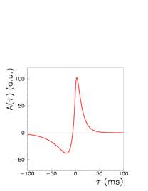
Figure 1: The learning window $A(\tau)$ used in the learning rule to model STDP, introduced and motivated by [32], $A(\tau)=a_{p}e^{-\tau/T_{p}}-a_{D}e^{-\eta\tau/T_{p}}$ if $\tau>0$, $A(\tau)=a_{p}e^{\eta\tau/T_{D}}-a_{D}e^{\tau/T_{D}}$ if $\tau<0$, with $a_{p}=\gamma\,[1/T_{p}+\eta/T_{D}]^{-1}$, $a_{D}=\gamma\,[\eta/T_{p}+1/T_{D}]^{-1}$, $T_{p}=10.2$ ms, $T_{D}=28.6$ ms, $\eta=4$, $\gamma=42$.

Figure 2: a) Plot of the self-sustained dynamics of the fully connected network with $N=500$ and $P=5$. The dynamics of the network, after a transient, is periodic of period $T=8\tau$. Different colors represent the value of $\lfloor 4t_{i}/T\rfloor\bmod 4$, where $t_{i}$ is time at which the neuron $i$ start to fire (black if neuron is firing at $t=0$). In this case the times $t_{i}$ are highly correlated with the phases $\phi_{i}^{1}$, which means that the pattern $\mu=1$ is well retrieved, and the overlap $m_{1}(t)$ is large. b) The same network with $P=50$. In this case the pattern is not retrieved, and the overlap is of order $\sqrt{1/N}$.

After the learning phase, we initialize the network with a given initial condition $\sigma_{i}(0)$, and perform a zero temperature spontaneous dynamics,

$$\sigma_{i}(t+\tau)=\operatorname{sign}\left[\sum_{j\neq i}J_{ij}\sigma_{j}(t)\right]$$ (5)

with $\tau$ the unit step of time. Due to the shape of the response function $\operatorname{sign}(x)$, if all the connections $J_{ij}$ are multiplied by the same positive constant, the dynamics is unchanged. Therefore, the learning time $t_{\text{max}}$ and the amplitude of the learning function $A(\tau)$ are immaterial.

In order to measure the similarity between the network activity during retrieval mode, and the stored phase-coded pattern $\mu$, we define the overlap

$$m^{\mu}(t)=\frac{1}{N}\sum_{i=1}^{N}\sigma_{i}(t)e^{i\phi_{i}^{\mu}}.$$ (6)

When the retrieval is perfect, $\sigma_{i}(t)=f(\tilde{\omega}t-\phi^{\mu}_{i})$, with an output angular velocity $\tilde{\omega}$ that is in general different from the input $\omega^{\mu}$. In this case $m^{\mu}(t)=\tilde{f}_{1}e^{i\tilde{\omega}t}$, where $|\tilde{f}_{1}|\simeq 0.64$ for the function (2). When the retrieval is not perfect, the modulus $|m^{\mu}(t)|$ after a transient goes to a constant value lower than the maximal one. Finally, if the network is not able to reproduce the pattern, the overlap becomes after a transient of order $1/\sqrt{N}$. The modulus of $m^{\mu}(t)$ is therefore an order parameter which measure how much the network dynamics match the stored phase-coded pattern $\mu$. Note that the output frequency $\tilde{\omega}/2\pi$ depends on the input frequency $\omega^{\mu}/2\pi$, and on the degree of asymmetry of the learning function $A(\tau)$. If $\tilde{\omega}$ is different from $\omega^{\mu}$, and $|m^{\mu}(t)|$ is high, it means that the phase-coded stored pattern $\mu$ is replayed at a frequency different from the one used to store it, i.e. at a different time scale, but with the same phase relationship. In Fig. 2a we show the dynamics of a network of $N=500$ neurons, with all the $N(N-1)$ connections activated, and with $P=5$ patterns encoded at input frequency $\omega^{\mu}/2\pi=10$ Hz. The network is initialized with a high overlap with the pattern $\mu=1$, setting

$$\sigma_{i}(0)=\left\{\begin{array}[]{ll}1&\mbox{if $0<\phi_{i}^{1}<\pi$},\\ -1&\mbox{if $\pi<\phi_{i}^{1}<2\pi$}.\end{array}\right.$$ (7)

Each segment represent a time interval in which the neuron $i$ is firing, that is $\sigma_{i}(t)=1$, with the neurons ordered on the vertical axis by the value of the phase of the first pattern $\phi_{i}^{1}$. In this case the pattern $\mu=1$ has been retrieved, and the overlap $m^{1}(t)$ has modulus $|m^{1}(t)|\simeq 0.63$ at long times. In Fig. 2b we show the same network with $P=50$ patterns encoded. In this case the pattern is not retrieved, and the overlap has modulus $|m^{1}(t)|\simeq 0.07$.

Figure 3: a) Storage capacity of the network, as a function of the fraction of connections $z/N$ and the number of patterns per neuron $P/N$, in the region of low connectivity, with $N=40000$ neurons. Solid (empty) circles represent points where the network is (is not) able to retrieve patterns. The network with $N=4000$ gives the same result (within errors). In this region of low $z/N$ the capacity is proportional to the number of connections. b) Storage capacity in the entire range of $z/N$, with $N=4000$ neurons. For clarity only a spline separating the encodable and the not-encodable region is shown. Inset: comparison between the $N=4000$ and the $N=40000$ cases for two values of $z/N$. The dashed line in all figures corresponds to $P=0.24\,z$.

We define the capacity $P_{\text{max}}$ of the network as the maximum number of patterns encodable in the network, and retrievable with an overlap greater than $0.2$. We have first studied the capacity of the network as a function of the number of connections, in the case of a fraction $\gamma=1$ of long range connections. As the probability to create a long range connections is independent on the distance of the neurons, in this case the network is completely random. We therefore consider a network of $N$ neurons, and create a connection from each neuron to a number $z$ of randomly chosen neurons, with $0<z<N$. We then look if the network is able to encode $P$ (random) pattern, and retrieve one of them subsequently. We initialize the network with an high overlap with one of the patterns, as in Eq. (7), and simulate the dynamics in Eq. (5) up to a time $t=2\times 10^{5}$ in Monte Carlo steps, looking if the overlap with the chosen pattern remains higher than $0.2$. The experiment is repeated with three different sets of $P$ patterns. In Fig. 3a the result is shown for $N=40000$. Solid (empty) circles represent points where the network was (was not) able to retrieve a pattern at least two times out of three. In practice, for all points considered, the network either was always able to retrieve the pattern (three times out of three), or never (zero times out of three). Furthermore, retrieved patterns had always an overlap greater than $0.36$, while not retrieved ones had an overlap lower than $0.08$. Results for $N=4000$ were practically the same, with a small number of points near the separation between encodable and not encodable region showing some fluctuations (retrieving the pattern one or two times out of three). Note that, in the range of values of $z/N$ considered in Fig. 3a, the maximum capacity $P_{\text{max}}$ is well described by a linear function of the connectivity, $P_{\text{max}}=0.24\,z$.

In Fig. 3b, we show the results for the entire range of $z/N$, from zero to one. When $z/N$ is of the order of unity, the number of connections is of order $N^{2}$, so the simulation is too expensive for $N=40000$. We therefore study sistematically only the network with $N=4000$, but compare it with the case $N=40000$ for two values of $z/N$, finding a good agreement. For clarity we do not show the points simulated, but only a spline separating the encodable and the not-encodable region. The dashed line shows the limit of the capacity for low connectivity $z/N$, $P_{\text{max}}=0.24\,z$. It can be seen that, when the connectivity grows, there is a saturation effect, so that for $z\simeq N$ one finds $P_{\text{max}}/N\simeq 0.032$, and therefore $P_{\text{max}}\simeq 0.032\,z$.

Figure 4: a) Storage capacity as a function of the fraction of long range connections $\gamma$, for a fixed number of connections per node (dashed line) or for a fixed total cost of the connections (solid line). b) Relative clustering coefficient and path length as a function of $\gamma$.

To study the effects of short and long range connectivity, we have then analyzed the capacity of the network in the case of a fraction $\gamma$ of long range connections, and $(1-\gamma)$ of short range connections. The result is shown in Fig. 4a (dashed line), for $N=40000$ and $z=180$ ($z/N=0.0045$). Note that in this case the sphere containing the short range neurons has a radius $R\simeq 3.5$, while the side of the cubic box is $L\simeq 34$. The storage capacity, that is the maximum encodable number of pattern such that the retrieval gives an overlap greater than 0.2, goes from $P_{\text{max}}\simeq 0.11\,z$ for $\gamma=0$ (only local connections) to $P_{\text{max}}\simeq 0.24\,z$ for $\gamma=1$ (random network). This shows that the number of connections is not the only parameter that determines the capacity of the network. Long range (random) connections are more effective than short range ones in encoding patterns.

The topology of the biological networks has been shaped by the evolution, as a compromise between the effectiveness in realizing complex tasks, and cost minimizations. While long range connections are more effective than short range ones, they are of course more costly. The trade-off between these two requirements will produce a network with a finite fraction of long range connections. We therefore introduce a parameter $f$, that represents the cost of a long range connections with respect to a short range one, and we consider a network with $(1-\gamma)z$ local connections, with neurons chosen randomly within those at distance lower than $R$, and $\gamma z/f$ long range connections, with neurons chosen randomly in the whole system. Varying $\gamma$, in this case it is not the connectivity that is constant, but the total cost of the connections. The storage capacity as a function of $\gamma$ is shown in Fig. 4a (solid line), for the case $f=3$. The maximum capacity of the network is realized with $\gamma\simeq 0.5$, that corresponds to about $25\%$ of long range connections over the total of the connections. To characterize the network, we have also calculated for the different values of $\gamma$ the clustering coefficient $C$, defined as the probability that two neurons, that are connected to a third neuron, are themselves connected, and the mean path length $\lambda$, defined as the minimum number of connections needed to go from a node to another node, averaged over all pairs of nodes. In Fig.4b, we show the relative clustering coefficient $(C-C_{1})/(C_{0}-C_{1})$, and path length $(\lambda-\lambda_{1})/(\lambda_{0}-\lambda_{1})$, where the quantities with subscripts 0 and 1 refer to the cases $\gamma=0$ and $\gamma=1$ respectively. Note that the clustering coefficient decreases much more slowly than the path length, giving rise to a large region where the clustering coefficient is not much lower than that for local connections only, while the path length is almost as low as in the random network. The network therefore, in the region of intermediate $\gamma$ that corresponds to optimal capacity, is of a small-world type [27].

In this paper we studied the storage and recall of patterns in which information is encoded in the phase-based timing of firing relative to the cycle. We proposed a STDP-based learning rule, and we analyzed the its ability to memorize multiple phase-coded patterns, such that the spontaneous dynamics of the network selectively gives sustained activity which matches one of the stored phase-coded patterns, depending on the initialization of the network. Our work generalizes the Hopfield model, to dynamical periodic states, characterized by the relative phases of the neurons.

We have studied the storage capacity for different degrees of sparseness and topologies of the connections. Changing the proportion $\gamma$ between short-range and long-range connections, we go from a three-dimensional network with only nearest-neighbors connections ($\gamma=0$) to a random network ($\gamma=1$). Small but finite values of $\gamma$ give a “small world” topology, similar to that found in many areas of nervous system.

We find that in the case of only short range connections the capacity is lowest, while in the case of only long range connections, that corresponds to a completely random network, the capacity is highest. Moreover, a small but finite fraction of long range connection is enough to enhance the capacity highly, with respect to the short range case. Therefore if the cost of the connections is taken in account, with long range connections more costly than short range ones, than the optimal capacity will be given by a small fraction of long range connections, that corresponds to a small-world topology.

This is in agreement with the observation that small-world attributes, with high clustering coefficient and short path length, was found across multiple spatial scales of cortical organization [33, 31]. This property, first found in C. elegans, is highly conserved over different type of measurement, and across different species, including cat, monkey and humans, for both functional and anatomical networks [28].

References

- [1] \NameBuzsaki G. Draguhn A. \REVIEWScience 30420041926.
- [2] \NameSinger W. \REVIEWNeuron 24199949.
- [3] \NameFries N., Nikolić D. Singer W. \REVIEWTrends in Neurosciences 302007309.
- [4] \NamePastalkova E., Itskov V., Amarasingham A. Buzsáki G. \REVIEWScience 32120081322.
- [5] \NameSiegel M., Warden M. R. Miller E. K. \REVIEWProc Natl Acad Sci USA 106200921341.
- [6] \NameO’Keefe J. Recce M. L. \REVIEWHippocampus 31993317.
- [7] \NameHuxter J., Burgess N. O’Keefe J. \REVIEWNature 4252003828.
- [8] \NameGeisler C., Robbe D., Zugaro M., Sirota A. Buzsaki G. \REVIEWProc Natl Acad Sci USA 10420078149.
- [9] \NamePerez-Orive J., Mazor O., Turner G. C., Cassenaer S., Wilson R. I. Laurent G. \REVIEWScience 2972002359.
- [10] \NameMontemurro M. A., Rasch M. J., Murayama Y., Logothetis N. K. Panzeri S. \REVIEWCurrent Biology 182008375.
- [11] \NameKayser C., Montemurro M. A., Logothetis N. K. Panzeri S. \REVIEWNeuron 612009597.
- [12] \NamePanzeri S., Brunel N., Logothetis N. Kayser C. \REVIEWTrends in Neurosciences 332010111.
- [13] \NameScarpetta S., Zhaoping L. Hertz J. \REVIEWNeural Computation 1420022371.
- [14] \NameLengyel M., Kwag J., Paulsen O. Dayan P. \REVIEWNature Neuroscience 820051677.
- [15] \NameMemmesheimer R. M. Timme M. \REVIEWPhys. Rev. Lett. 972006188101.
- [16] \NameYoshioka M., Scarpetta S. Marinaro M. \REVIEWPhys. Rev. E 752007051917.
- [17] \NameYoshioka M. \REVIEWPhys. Rev. Lett. 1022009158102.
- [18] \NameBush D., Philippides A., Husbands P. O’Shea M. \REVIEWPLoS Comput Biol. 62010e1000839.
- [19] \NameMasquelier T., Hugues E., Deco G. Thorpe S. \REVIEWJ. Neurosci. 29200913484.
- [20] \NameFlight M. H. \REVIEWNature Reviews Neuroscience 102010834.
- [21] \NameMarkram H., Lubke J., Frotsher M. Sakmann B. \REVIEWScience 2751997213.
- [22] \NameBi G. Q. Poo M. M. \REVIEWJ. Neurosci. 18199810464.
- [23] \NameCaporale N. Dan Y. \REVIEWAnnu. Rev. Neurosci. 31200825.
- [24] \NameSiostrom P. J. \REVIEWFront. Syn. Neurosc. 220104.
- [25] \NameKoch C. Laurent G. \REVIEWScience 284199996.
- [26] \NameLaughlin S. B. Sejnowski T. J. \REVIEWScience 30120031870.
- [27] \NameWatts D. J. Strogatz S. H. \REVIEWNature 3931998440.
- [28] \NameBullmore E. Sporns O. \REVIEWNat. Rev. Neurosci. 202009186.
- [29] \NameLatora V. Marchiori M. \REVIEWEur. Phys. J. B 322003249.
- [30] \NameYu S., Huang D., Singer W. Nikolić D. \REVIEWCerebral Cortex 1820082891.
- [31] \NameSporns O. Zwi J. D. \REVIEWNeuroinformatics 22004145.
- [32] \NameAbarbanel H., Huerta R. Rabinovich M. I. \REVIEWProc Natl Acad Sci USA 99200210132.
- [33] \NameSporns O., Chialvo D., Kaiser M. Hilgetag C. \REVIEWTrends in Cognitive Science 82004418.