Field theory of bicritical and tetracritical points. IV. Critical dynamics including reversible terms.

Abstract

This article concludes a series of papers (R. Folk, Yu. Holovatch, and G. Moser, Phys. Rev. E 78, 041124 (2008); 78, 041125 (2008); 79, 031109 (2009)) where the tools of the field theoretical renormalization group were employed to explain and quantitatively describe different types of static and dynamic behavior in the vicinity of multicritical points. Here, we give the complete two loop calculation and analysis of the dynamic renormalization-group flow equations at the multicritical point in anisotropic antiferromagnets in an external magnetic field. We find that the time scales of the order parameters characterizing the parallel and perpendicular ordering with respect to the external field scale in the same way. This holds independent whether the Heisenberg fixed point or the biconical fixed point in statics is the stable one. The non-asymptotic analysis of the dynamic flow equations shows that due to cancelation effects the critical behavior is described - in distances from the critical point accessible to experiments - by the critical behavior qualitatively found in one loop order. Although one may conclude from the effective dynamic exponents (taking almost their one loop values) that weak scaling for the order parameter components is valid, the flow of the time scale ratios is quite different and they do not reach their asymptotic values.

I Introduction

Three component antiferromagnets in three spatial dimensions in an external magnetic field in $z$ direction contain in their phase diagram two second order transition lines: (i) between the paramagnetic and the spin flop phase and (ii) between the antiferromagnetic and paramagnetic phase. The point where these two lines meet is a multicritical point which turned out to be either bicritical or tetracritical. Within the renormalization group (RG) theory the stability and attraction region of the static fixed point (FP) of the RG transformation determines, which kind of multicritical behavior is realized. For the bicritical point it is the Heisenberg FP, for the tetracritical point it is the biconical one. The stabilty of a FP depends on the system’s global features as the space and order parameter (OP) dimensions $d$ and $n$. In $d=3$, the case considered here, the biconical FP is stable apart from a restricted attraction region of the Heisenberg FP . The static phase transition on each of the phase transition lines belongs for (i) to an isotropic Heisenberg model with $n_{\perp}=2$ and for (ii) to Heisenberg model with $n_{\|}=1$ konefi76 ; partI .

Concerning the dynamical universality classes the transition (i) belongs to the class described by model F and (ii) belongs to the model C class (for the notation see review ). At the multicritical point the critical behavior is described by a new universality class both in statics and dynamics. The interesting feature of these systems is that all the different OPs characterizing the ordered phase are physically accessible. This is most important for the dynamical behavior since the only other example belonging to model F is the superfluid transition in ⁴He where the OP (the complex macroscopic wave function of the condensate josephson66 ) is experimentally not accessible hh69 . Here the OPs are the components of the staggered magnetization. Their correlations (static and dynamical) can be measured by neutron scattering.

A complete description of the critical dynamics near the multicritical point mentioned above has to take into account the slow dynamical densities which are the OPs and the conserved densities present in the system. Due to the external magnetic field the only conserved density which has to be taken into account is the magnetization in direction of the external field. A derivation of the dynamical equations follows along the usual steps calculating the reversible terms from the non-zero Poisson brackets, introducing irreversible terms present also in the hydrodynamic limit, dropping irrelevant terms and taking into account terms arising in the renormalization procedure (see e.g. the review review ). Such a dynamical model has already been considered in dohmjanssen77 ; dohmmulti83 ; dohmKFA by RG theory and it was argued that due to nonanalytic terms in $\varepsilon=4-d$ a FP in two loop order qualitative different from the one loop FP is found. The result of the one loop calculations is that the time scales of the parallel and perpendicular components of the staggered magnetization scale differently whereas calculated in two loop order they scale similar although the FP value of the timescale ratio of the two components cannot be found by $\varepsilon$ expansion and might be very small in $d=3$ namely of ${\cal O}(10^{-86})$. It was argued that the terms leading to the singular behavior in $\varepsilon$ do not contribute to the FP value of the mode coupling. The calculations of the RG-functions in dohmjanssen77 where not complete in two loop order (they took into account only the terms which lead to the nonanalytic behavior in $\varepsilon$). At that time also the Heisenberg FP (named $\cal{H}$) was considered to be the stable static one, whereas it turned out in two loop order (resummed) that it is the biconical FP (named $\cal{B}$) partI .

FP values in …	$w^{\star}_{\|}$	$w^{\prime\star}_{\perp}$	$v^{\prime\star}$	$f^{\star}_{\perp}$
${\cal B_{C}}$ partIII	$0.76$	$\gg 1$	$\sim 0$	-
${\cal B}$ 1-loop	$0$	$1.555$	$0$	$1.086$
${\cal B}$ 2-loop	$0$	$0$	$\sim 0$	$1.131$
model C C	$0.49$	-	-	-
model F F	-	0	-	$0.834$

Table 1: Dynamical FP values (zeros of the corresponding dynamical $\beta$-functions) at $d=3$ of different models for the time scale ratios $w^{\star}_{\|},\,w^{\prime\star}_{\perp},\,v^{\prime\star}$ and the mode coupling constant $f^{\star}_{\perp}$. The 2nd and 3rd lines quote results of this paper found in the biconical static FP for the tetracritical behavior of the dynamical model that takes into account reversible terms. They are compared with the two loop results found in the model C multicritical point partIII as well as in the critical points of model C for the one component OP C and of model F for the two component order parameter F .

A summary of the results obtained so far for the FPs characterizing dynamical behavior is given in table 1. Neglecting the reversible terms one is left with a purely relaxational dynamics. Then the asymptotic dynamical critical behavior is characterized by the FP values of the independent time scale ratios of the system. These are the following time scale ratios: (1) the ratio $w_{\|}$ between the relaxation rate of the staggered magnetization parallel to the external field and the diffusive transport coefficient of the magnetization parallel to the external field; (2) the ratio $w^{\prime}_{\perp}$ between the real part of the relaxation rate of the staggered magnetization perpendicular to the external field and the diffusive transport coefficient of the magnetization parallel to the external field. In addition we introduce the ratio $v^{\prime}$ between the two components of the real relaxation rates of the two OPs in order to compare their dynamic scaling behavior. A non-zero finite value of the time scale ratio means that the two involved densities scale with the same exponent. If all time scale ratios are non-zero and finite, one speaks of strong dynamic scaling, otherwise of weak dynamic scaling. Especially of interest is the behavior of the scaling of the two components of the OP indicated by the FP value of $v^{\prime}$. In the third line of table 1 the two loop order result shows weak dynamic scaling between the OPs and the conserved density but strong scaling between the OP components. However since the FP value time scale ratio $v^{\prime}$ is almost zero, the critical behavior is dominated by non-asymptotic effects. For comparison the FP values for the case of model C for the one component OP C and for model F for the two component order parameter F are included. They are the limiting cases when the two OPs characterizing the multicritical behavior would decouple in statics and dynamics.

In the first line of table 1 the results for the multicritical dynamical FP $\cal{B}_{C}$ values taking into account the static coupling of the OP to the conserved density are displayed (see partIII ). All time scale ratios are non-zero and finite but since $w^{\prime\star}_{\perp}$ is very large ($v^{\prime\star}$ almost zero) the observable behavior in the vicinity of the multicritical point is predicted to be dominated by non-asymptotic effects and strong scaling is not observable partIII . In the second line the results of a one loop RG calculation with reversible terms for the biconical FP are given. The FP value of the mode coupling parameter $f_{\perp}$ is finite but since $w^{\star}_{\|}=0$ the critical dynamics is characterized by weak dynamic scaling and the two components of the OP scale different. A similar result for the Heisenberg FP was found in dohmjanssen77 . In the third line the results found in this paper are shown, indicating weak scaling between the conserved density and the components of the OP, but strong scaling between the parallel and perpendicular components of the OP. Since the FP value of the time scale ratio between the component $v^{\prime\star}$ is almost zero but definitively different from zero it is expected that non-asymptotic behavior is dominant.

This article concludes a series of papers partI ; partII ; partIII (henceforth cited as papers I, II, and III) where the tools of the field theoretical RG were employed to explain and quantitatively describe different types of static and dynamic behavior in the vicinity of multicritical points. A short account of the results presented here was given in letter . The statics and dynamics were treated in Refs. partI and partII ; partIII , respectively. First, purely relaxational dynamics was considered (paper II) and later, in paper III, these results served as a basis to consider how an account of magnetization conservation modifies dynamical behavior. The goal of the current study is more ambitious: we will analyze a complete set of dynamical equations of motion taking into account reversible terms huber74 ; huberrag76 and give a comprehensive description of dynamical behavior in the vicinity of multicritical points in two loop order. The paper is organized as follows: In section II the dynamic model is defined followed by a the definitions of the dynamical functions considered in section III. The renormalization and corresponding RG-functions are presented in section IV and V respectively. The two loop results of our calculations for these dynamic RG-functions are given in section VI. The one loop approximation for the dynamic is discussed in section VII. In the next section VIII we consider the asymptotic properties of the two loop RG-functions leading to the general asymptotic results in section IX. We then present the results expected in the asymptotic subspace, section X. The non-asymptotic behavior, obtained by looking at the region further away from the multicritical point, is shown in section XI, a conclusion XII ends the paper. In Appendices calculational details for some intermediate steps of the RG calculation are presented.

II Model equations of the antiferromagnet in an external field

The non-conserved OP $\vec{\phi}_{0}$ of an isotropic antiferromagnet is given by the three dimensional vector

$$\vec{\phi}_{0}=\left(\begin{array}[]{c}\phi_{0}^{x}\\ \phi_{0}^{y}\\ \phi_{0}^{z}\end{array}\right)$$ (1)

of the staggered magnetization, which is the difference of two sublattice magnetizations. An external magnetic field applied to the ferromagnet induces an anisotropy to the system. The OP splits into two OPs, $\vec{\phi}_{\perp 0}$ perpendicular to the field, and $\vec{\phi}_{\|0}$ parallel to the external field. Assuming the $z$-axis in direction of the external magnetic field, the two OPs are

$$\vec{\phi}_{\perp 0}=\left(\begin{array}[]{c}\phi_{0}^{x}\\ \phi_{0}^{y}\end{array}\right)\ ,\qquad\phi_{\|0}=\phi_{0}^{z}$$ (2)

In addition the $z$-component of the magnetization $m_{0}$ has to be taken into account for the dynamics and therefore has to be included in statics although there it could be integrated out and does not change the asymptotic static critical behavior. Thus the static critical behavior of the system is described by the functional

$${\cal H}\!=\!\int\!d^{d}x\Bigg{\{}\frac{1}{2}\mathring{r}_{\perp}\vec{\phi}_{\perp 0}\cdot\vec{\phi}_{\perp 0}+\frac{1}{2}\sum_{i=1}^{d}\nabla_{i}\vec{\phi}_{\perp 0}\cdot\nabla_{i}\vec{\phi}_{\perp 0}$$

$$+\frac{1}{2}\mathring{r}_{\|}{\phi}_{\|0}{\phi}_{\|0}+\frac{1}{2}\sum_{i=1}^{d}\nabla_{i}\phi_{\|0}\nabla_{i}\phi_{\|0}+\frac{\mathring{u}_{\perp}}{4!}\Big{(}\vec{\phi}_{\perp 0}\cdot\vec{\phi}_{\perp 0}\Big{)}^{2}$$

$$+\frac{\mathring{u}_{\|}}{4!}\Big{(}\phi_{\|0}\phi_{\|0}\Big{)}^{2}+\frac{2\mathring{u}_{\times}}{4!}\Big{(}\vec{\phi}_{\perp 0}\cdot\vec{\phi}_{\perp 0}\Big{)}\Big{(}\phi_{\|0}\phi_{\|0}\Big{)}\Bigg{\}}$$ (3)

$$+\frac{1}{2}m_{0}^{2}+\frac{1}{2}\mathring{\gamma_{\perp}}m_{0}\vec{\phi}_{\perp 0}\cdot\vec{\phi}_{\perp 0}+\frac{1}{2}\mathring{\gamma_{\|}}m_{0}\phi_{\|0}\phi_{\|0}-\mathring{h}m_{0}\Bigg{\}}\ ,$$

with familiar notations for bare couplings $\{\mathring{u},\mathring{\gamma}\}$, masses $\{\mathring{r}\}$ and field $\mathring{h}$ partI ; partII . The critical dynamics of relaxing OPs coupled to a diffusing secondary density is governed by the following equations of motion dohmjanssen77 :

$$\frac{\partial\phi_{\perp 0}^{\alpha}}{\partial t} = -\mathring{\Gamma}^{\prime}_{\perp}\frac{\delta{\mathcal{H}}}{\delta\phi_{\perp 0}^{\alpha}}+\mathring{\Gamma}^{\prime\prime}_{\perp}\epsilon^{\alpha\beta z}\frac{\delta{\mathcal{H}}}{\delta\phi_{\perp 0}^{\beta}}$$ (4)

$$+ \mathring{g}\ \epsilon^{\alpha\beta z}\phi_{\perp 0}^{\beta}\frac{\delta{\mathcal{H}}}{\delta m_{0}}+\theta_{\phi_{\perp}}^{\alpha}\ ,$$

$$\frac{\partial\phi_{\|0}}{\partial t} = -\mathring{\Gamma}_{\|}\frac{\delta{\mathcal{H}}}{\delta\phi_{\|0}}+\theta_{\phi_{\|}}\,,$$ (5)

$$\frac{\partial m_{0}}{\partial t} = \mathring{\lambda}\nabla^{2}\frac{\delta{\mathcal{H}}}{\delta m_{0}}+\mathring{g}\ \epsilon^{\alpha\beta z}\phi_{\perp 0}^{\alpha}\frac{\delta{\mathcal{H}}}{\delta\phi_{\perp 0}^{\beta}}+\theta_{m}\,,$$ (6)

with the Levi-Civita symbol $\epsilon^{\alpha\beta z}$. Here $\alpha,\beta=x,y$ and the sum over repeated indices is implied.

The dynamical equations describe the dynamics of an antiferromagnet with the usual Lamor precession terms for the alternating magnetization and relaxational terms. Due to the static coupling to the conserved magnetization additional Lamor terms arise together with a diffusive term for the magnetization. Renormalization considerations lead on one hand to a neglection of several Lamor terms and on the other hand create an additional reversible term (the second term on the right hand side of Eq. 5)) not present in the usual dynamics of antiferromagnets antiferro .

Combining the kinetic coefficients of the OP to a complex quantity, $\mathring{\Gamma}_{\perp}=\mathring{\Gamma}_{\perp}^{\prime}+\mbox{i}\mathring{\Gamma}_{\perp}^{\prime\prime}$, the imaginary part constitutes a precession term created by the renormalization procedure even if it is absent in the background. The kinetic coefficient $\mathring{\lambda}$ and the mode coupling $\mathring{g}$ are real. The stochastic forces $\vec{\theta}_{\phi_{\perp}}$, $\vec{\theta}_{\phi_{\|}}$ and $\theta_{m}$ fulfill Einstein relations

$$\langle\theta_{\phi_{\perp}}^{\alpha}(\vec{x},t)\ \theta_{\phi_{\perp}}^{\beta}(\vec{x}^{\prime},t^{\prime})\rangle\!\!\! = \!\!\!2\mathring{\Gamma}^{\prime}_{\perp}\delta(\vec{x}-\vec{x}^{\prime})\delta(t-t^{\prime})\delta^{\alpha\beta}\ ,$$ (7)

$$\langle\theta_{\phi_{\|}}(\vec{x},t)\ \theta_{\phi_{\|}}(\vec{x}^{\prime},t^{\prime})\rangle\!\!\! = \!\!\!2\mathring{\Gamma}_{\|}\delta(\vec{x}-\vec{x}^{\prime})\delta(t-t^{\prime})\ ,$$ (8)

$$\langle\theta_{m}(\vec{x},t)\ \theta_{m}(\vec{x}^{\prime},t^{\prime})\rangle\!\!\! = \!\!\!-2\mathring{\lambda}\nabla^{2}\delta(\vec{x}-\vec{x}^{\prime})\delta(t-t^{\prime})\ .$$ (9)

In view of dynamical calculations it is more convenient to deal with a scalar complex order parameter $\psi_{0}=\psi_{0}^{\prime}+\mbox{i}\psi_{0}^{\prime\prime}$ instead of the real two-dimensional OP $\vec{\phi}_{\perp 0}$ in (2). Thus we may introduce

$$\psi_{0}=\phi_{0}^{x}-\mbox{i}\phi_{0}^{y}\ ,\qquad\psi_{0}^{+}=\phi_{0}^{x}+\mbox{i}\phi_{0}^{y}$$ (10)

as OP of the perpendicular components. The superscript ⁺ denotes complex conjugated quantities also in the following equations. In addition to the two OPs the $z$-component of the magnetization, which is the sum of the two sublattice magnetizations, has to be considered as conserved secondary density $m_{0}$.

Expressed in terms of the above densities the dynamic equations take the form

$$\frac{\partial\psi_{0}}{\partial t}\!\! = \!\!-2\mathring{\Gamma}_{\perp}\frac{\delta H}{\delta\psi_{0}^{+}}+\mbox{i}\psi_{0}\mathring{g}\frac{\delta H}{\delta m_{0}}+\theta_{\psi}\,,$$ (11)

$$\frac{\partial\psi_{0}^{+}}{\partial t}\!\! = \!\!-2\mathring{\Gamma}_{\perp}^{+}\frac{\delta H}{\delta\psi_{0}}-\mbox{i}\psi_{0}^{+}\mathring{g}\frac{\delta H}{\delta m_{0}}+\theta_{\psi}^{+}\,,$$ (12)

$$\frac{\partial\phi_{\|0}}{\partial t}\!\! = \!\!-\mathring{\Gamma}_{\|}\frac{\delta H}{\delta\phi_{\|0}}+\theta_{\phi_{\|}}\,,$$ (13)

$$\frac{\partial m_{0}}{\partial t}\!\! = \!\!\mathring{\lambda}\nabla^{2}\frac{\delta H}{\delta m_{0}}-2\mathring{g}\Im[\psi_{0}^{+}\nabla^{2}\psi_{0}]+\theta_{m}\,.$$ (14)

Due to the fact that the stochastic forces $\theta_{\phi_{\perp}}^{\alpha}$ in (4) are $\delta$-correlated and fulfil the Einstein relations, similar properties hold also for the stochastic forces $\theta_{\psi}$:

$$\langle\theta_{\psi}(x,t)\ \theta_{\psi}^{+}(x^{\prime},t^{\prime})\rangle=4\mathring{\Gamma}_{\perp}^{\prime}\ \delta(x-x^{\prime})\delta(t-t^{\prime})\,.$$ (15)

The critical behavior of the thermodynamic derivatives follows from the extended static functional (the functional (II) written in the variables intoduced in (10))

$${\cal H}={\cal H}^{(0)}+{\cal H}^{(int)}$$ (16)

with a Gaussian part

$${\cal H}^{(0)}\!=\!\int\!d^{d}x\Bigg{\{}\frac{1}{2}\mathring{\tilde{r}}_{\perp}\psi_{0}^{+}\psi_{0}+\frac{1}{2}(\nabla\psi_{0}^{+})(\nabla\psi_{0})$$

$$+\frac{1}{2}\mathring{\tilde{r}}_{\|}\phi_{\|0}^{2}+\frac{1}{2}(\nabla\phi_{\|0})^{2}+\frac{1}{2}m_{0}^{2}-\mathring{h}m_{0}\Bigg{\}}\ ,$$ (17)

and an interaction part

$${\cal H}^{(int)}\!=\!\int\!d^{d}x\Bigg{\{}\frac{\mathring{\tilde{u}}_{\perp}}{4!}(\psi_{0}^{+}\psi_{0})^{2}+\frac{\mathring{\tilde{u}}_{\|}}{4!}\phi_{\|0}^{4}+\frac{2\mathring{\tilde{u}}_{\times}}{4!}\psi_{0}^{+}\psi_{0}\phi_{\|0}^{2}$$

$$+\frac{1}{2}\mathring{\gamma}_{\perp}m_{0}\psi_{0}^{+}\psi_{0}+\frac{1}{2}\mathring{\gamma}_{\|}m_{0}\phi_{\|0}^{2}\Bigg{\}}\ .$$

The above static functional may be reduced to the Ginzburg-Landau-Wilson (GLW) functional with complex OP by considering an appropriate Boltzmann distribution and integrating out the secondary density. One obtains

$${\cal H}_{GLW}\!=\!\int\!d^{d}x\Bigg{\{}\frac{1}{2}\mathring{r}_{\perp}\psi_{0}^{+}\psi_{0}+\frac{1}{2}(\nabla\psi_{0}^{+})(\nabla\psi_{0})$$

$$+\frac{1}{2}\mathring{r}_{\|}\phi_{\|0}^{2}+\frac{1}{2}(\nabla\phi_{\|0})^{2}$$

$$+\frac{\mathring{u}_{\perp}}{4!}(\psi_{0}^{+}\psi_{0})^{2}+\frac{\mathring{u}_{\|}}{4!}\phi_{\|0}^{4}+\frac{2\mathring{u}_{\times}}{4!}\psi_{0}^{+}\psi_{0}\phi_{\|0}^{2}\Bigg{\}}\ .$$ (19)

The parameters $\{\mathring{r}\}\equiv\mathring{r}_{\perp},\mathring{r}_{\|}$ and $\{\mathring{u}\}\equiv\mathring{u}_{\perp},\mathring{u}_{\|},\mathring{u}_{\times}$ in (II) are related to the corresponding parameters of the extended static functional (16) by

$$\mathring{r}_{\perp}=\mathring{\tilde{r}}_{\perp}+\mathring{\gamma}_{\perp}\mathring{h}\ ,\qquad \mathring{u}_{\perp}=\mathring{\tilde{u}}_{\perp}-3\mathring{\gamma}_{\perp}^{2}\ ,$$ (20)

$$\mathring{r}_{\|}=\mathring{\tilde{r}}_{\|}+\mathring{\gamma}_{\|}\mathring{h}\ ,\qquad \mathring{u}_{\|}=\mathring{\tilde{u}}_{\|}-3\mathring{\gamma}_{\|}^{2}\ ,$$ (22)

$$\mathring{u}_{\times}=\mathring{\tilde{u}}_{\times}-3\mathring{\gamma}_{\perp}\mathring{\gamma}_{\|}\ .$$

The property that the static critical behavior does not depend on the secondary densities, which can be integrated out in (16), leads to relations between the correlation functions of the secondary densities and the OP correlation functions. These relations and their derivations have been extensively discussed in paper III with real OP functions $\vec{\phi}_{\perp 0}$ and $\phi_{\|0}$. Because the derivation of the relations is independent of the type of OP (real or complex), all of the relations remain valid and can be taken over from paper III. Therefore we will not repeat them here.

III Dynamic correlation and vertex functions

The Fourier transformed dynamic correlation functions of the two OPs are usually introduced as

$$\mathring{C}_{\psi\psi^{+}}(\{\xi\},k,\omega)=\!\!\int\!\!d^{d}x\!\!\int\!\!dte^{-ikx+i\omega t}\langle\psi_{0}(x,t)\psi_{0}^{+}(0,0)\rangle_{c}$$ (23)

$$\mathring{C}_{\phi_{\|}\phi_{\|}}(\{\xi\},k,\omega)=\!\!\int\!\!d^{d}x\!\!\int\!\!dte^{-ikx+i\omega t}\langle\phi_{\|0}(x,t)\phi_{\|0}(0,0)\rangle_{c}$$ (24)

All functions depend on the two correlation lengths $\xi_{\perp}$ and $\xi_{\|}$, which is indicated by $\{\xi\}$ in a short notation. $\langle AB\rangle_{c}=\langle AB\rangle-\langle A\rangle\langle B\rangle$ denotes the cumulant. The averages are calculated with a propability density including a dynamic functional, which can be constituted from the dynamic equations (11) - (14). In the considered approach of bauja76 for every density auxiliary densities are introduced accordingly. They are denoted as $\tilde{\psi}_{0}^{+}$, $\tilde{\psi}_{0}$, $\tilde{\phi}_{\|0}$ and $\tilde{m}_{0}$. The dynamic correlation functions of the order parameters are connected to dynamic vertex functions via

$$\mathring{C}_{\psi\psi^{+}}(\{\xi\},k,\omega)=-\frac{\mathring{\Gamma}_{\tilde{\psi}\tilde{\psi}^{+}}(\{\xi\},k,\omega)}{\left|\mathring{\Gamma}_{\psi\tilde{\psi}^{+}}(\{\xi\},k,\omega)\right|^{2}}\,,$$ (25)

$$\mathring{C}_{\phi_{\|}\phi_{\|}}(\{\xi\},k,\omega)=-\frac{\mathring{\Gamma}_{\tilde{\phi}_{\|}\tilde{\phi}_{\|}}(\{\xi\},k,\omega)}{\left|\mathring{\Gamma}_{\phi_{\|}\tilde{\phi}_{\|}}(\{\xi\},k,\omega)\right|^{2}}\,,$$ (26)

where the two-point vertex functions appearing on the right hand side in the above expression have to be calculated within perturbation expansion. They are obtained by collecting all 1-particle irreducible Feynman graphs with corresponding external legs. A closer examination of the loop expansion reveals fomo02 that the dynamic response vertex functions $\mathring{\Gamma}_{\psi\tilde{\psi}^{+}}$ and $\mathring{\Gamma}_{\phi_{\|}\tilde{\phi}_{\|}}$ have the general structure

$$\mathring{\Gamma}_{\psi\tilde{\psi}^{+}}(\{\xi\},k,\omega) = \!\!-\,\,\mbox{i}\omega\mathring{\Omega}_{\psi\tilde{\psi}^{+}}(\{\xi\},k,\omega)$$ (27)

$$+ \!\!\mathring{\Gamma}_{\psi\psi^{+}}(\{\xi\},k)\mathring{\Gamma}^{(d)}_{\psi\tilde{\psi}^{+}}(\{\xi\},k,\omega)\,,$$

$$\mathring{\Gamma}_{\phi_{\|}\tilde{\phi}_{\|}}(\{\xi\},k,\omega) = \!\!-\,\,\mbox{i}\omega\mathring{\Omega}_{\phi_{\|}\tilde{\phi}_{\|}}(\{\xi\},k,\omega)$$ (28)

$$+ \!\!\mathring{\Gamma}_{\phi_{\|}\phi_{\|}}(\{\xi\},k)\mathring{\Gamma}_{\|}\,,$$

where $\mathring{\Gamma}_{\psi\psi^{+}}(\{\xi\},k)$ and $\mathring{\Gamma}_{\phi_{\|}\phi_{\|}}(\{\xi\},k)$ are the well known static two point vertex functions of the bicritical GLW-model with a complex OP. We want to remark that the static vertex functions in (27) and (28) are related by

$$\mathring{\Gamma}_{\psi\psi^{+}}(\{\xi\},k)=\frac{1}{2}\mathring{\Gamma}_{\perp\perp}^{(2,0)}(\{\xi\},k)$$ (29)

and

$$\mathring{\Gamma}_{\phi_{\|}\phi_{\|}}(\{\xi\},k)=\mathring{\Gamma}_{\|\|}^{(2,0)}(\{\xi\},k)$$ (30)

to the static vertex functions introduced in papers I–III for the model with real OPs. Thus the correlation lengths $\xi_{\perp}$ and $\xi_{\|}$ are now determined by

$$\xi_{\perp}^{2}(\{\mathring{r}\},\{\mathring{u}\})=\frac{\partial\ln\mathring{\Gamma}_{\psi\psi^{+}}(k,\{\mathring{r}\},\{\mathring{u}\})}{\partial k^{2}}\Bigg{|}_{k=0}\,,$$ (31)

$$\xi_{\|}^{2}(\{\mathring{r}\},\{\mathring{u}\})=\frac{\partial\ln\mathring{\Gamma}_{\phi_{\|}\phi_{\|}}(k,\{\mathring{r}\},\{\mathring{u}\})}{\partial k^{2}}\Bigg{|}_{k=0}\,.$$ (32)

$\mathring{\Omega}_{\psi\tilde{\psi}^{+}}$, $\mathring{\Gamma}^{(d)}_{\psi\tilde{\psi}^{+}}$ and $\mathring{\Omega}_{\phi_{\|}\tilde{\phi}_{\|}}$ are purely dynamic functions. The explicit expressions of these functions are given in appendix A, Eqs. (A) - (A). They determine also the dynamic vertex functions $\mathring{\Gamma}_{\tilde{\psi}\tilde{\psi}^{+}}$ and $\mathring{\Gamma}_{\tilde{\phi}_{\|}\tilde{\phi}_{\|}}$ in (25) and (26). A proper rearrangement of the perturbative contributions shows that the relations

$$\mathring{\Gamma}_{\tilde{\psi}\tilde{\psi}^{+}}(\{\xi\},k,\omega)=-2\Re\left[\mathring{\Omega}_{\psi\tilde{\psi}^{+}}(\{\xi\},k,\omega)\mathring{\Gamma}^{(d)}_{\psi\tilde{\psi}^{+}}(\{\xi\},k,\omega)\right]\,,$$ (33)

$$\mathring{\Gamma}_{\tilde{\phi}_{\|}\tilde{\phi}_{\|}}(\{\xi\},k,\omega)=-2\Gamma_{\|}\Re\left[\mathring{\Omega}_{\phi_{\|}\tilde{\phi}_{\|}}(\{\xi\},k,\omega)\right]$$ (34)

hold. $\Re[.]$ is the real part of the expression in the brackets.

Analogous to (23) and (24) the Fourier transformed dynamic correlation function of the secondary density is introduced as

$$\mathring{C}_{mm}(\{\xi\},k,\omega)=\!\!\int\!\!d^{d}x\!\!\int\!\!dte^{-ikx+i\omega t}\langle m_{0}(x,t)m_{0}(0,0)\rangle_{c}$$ (35)

The connection to the dynamic vertex functions is analogous to the case of the OP Eqs. (25 and (26):

$$\mathring{C}_{mm}(\{\xi\},k,\omega)=-\frac{\mathring{\Gamma}_{\tilde{m}\tilde{m}}(\{\xi\},k,\omega)}{\left|\mathring{\Gamma}_{m\tilde{m}}(\{\xi\},k,\omega)\right|^{2}}\,.$$ (36)

The dynamic response vertex function of the secondary density has the general structure

$$\mathring{\Gamma}_{m\tilde{m}}(\{\xi\},k,\omega)\!\! = \!\!-\mbox{i}\omega\mathring{\Omega}_{m\tilde{m}}(\{\xi\},k,\omega)$$ (37)

$$+ \!\!\mathring{\Gamma}_{mm}(\{\xi\},k)\mathring{\Gamma}^{(d)}_{m\tilde{m}}(\{\xi\},k,\omega)$$

where $\mathring{\Gamma}_{mm}(\{\xi\},k)$ is the static two point vertex function calculated with the extended static functional (16) which already has been introduced in paper III. A relation corresponding to (33) holds also for the dynamic vertex function of the secondary density. We have

$$\mathring{\Gamma}_{\tilde{m}\tilde{m}}(\{\xi\},k,\omega)=-2\Re\left[\mathring{\Omega}_{m\tilde{m}}(\{\xi\},k,\omega)\mathring{\Gamma}^{(d)}_{m\tilde{m}}(\{\xi\},k,\omega)\right]\,.$$ (38)

IV Renormalization

IV.1 Static renormalization

The renormalization of the GLW-functional (II) has been extensively discussed in paper I. The only difference in the present paper is that we now have to renormalize the complex OP $\psi_{0}$ instead of the real vector OP $\vec{\phi}_{\perp 0}$. We introduce the following renormalization factor

$$\psi_{0}=Z_{\psi}^{1/2}\psi\ ,\qquad\psi_{0}^{+}=Z_{\psi}^{1/2}\psi^{+}$$ (39)

where $Z_{\psi}$ is a real quantity and identical to $Z_{\phi_{\perp}}$ in paper I taken at $n_{\perp}=2$ and $n_{\|}=1$. This means

$$Z_{\psi}=Z_{\phi_{\perp}}\Big{|}_{n_{\perp}=2\atop n_{\|}=1}\,.$$ (40)

The renormalization of the parameters $\mathring{r}_{\perp}$, $\mathring{r}_{\|}$ and the couplings $\mathring{u}_{\perp}$, $\mathring{u}_{\|}$, $\mathring{u}_{\times}$ appearing in (II) is given in paper I (see Eqs. (16), (17) and (5)-(7)). In all relations one has to replace $Z_{\phi_{\perp}}$ by $Z_{\psi}$. All renormalization factors remain valid if one sets $n_{\perp}=2$ and $n_{\|}=1$. This is also true for the $Z$-matrix $\mbox{\boldmath$Z$}_{\phi^{2}}$ introduced in Eq.(10) of paper I and the additive renormalization $\mbox{\boldmath$A$}(\{u\})$ defined in Eq. (15) of paper I.

The renormalization of the parameters in the extended static functional (16) has been presented in paper III. As in the case of the bicritical GLW-model all $Z$-factors and relations between them remain valid if $Z_{\phi_{\perp}}$ therein is replaced by $Z_{\psi}$, and if one sets $n_{\perp}=2$ and $n_{\|}=1$ in explicit expressions.

IV.2 Dynamic renormalization

Within dynamics auxiliary densities $\tilde{\psi}_{0}$, $\tilde{\phi}_{\|0}$ and $\tilde{m}_{0}$ corresponding to the two OPs and the secondary density are introduced bauja76 . Instead of renormalization conditions we use the minimal subtraction scheme schloms as in the preceding papers II and III. The auxiliary density of the complex OP is multiplicatively renormalizable by introducing complex $Z$-factors:

$$\tilde{\psi}_{0}=Z_{\tilde{\psi}}^{1/2}\tilde{\psi}\ ,\qquad\tilde{\psi}_{0}^{+}=Z_{\tilde{\psi}^{+}}^{1/2}\tilde{\psi}^{+}$$ (41)

The complex renormalization factors in (41) fulfill the relation $Z_{\tilde{\psi^{+}}}=Z_{\tilde{\psi}}^{+}$. For the auxiliary densities of the single-component real OP and the secondary density the corresponding renormalization factors are introduced:

$$\tilde{\phi}_{\|0}=Z_{\tilde{\phi}_{\|}}^{1/2}\tilde{\phi}_{\|}\ ,\qquad\tilde{m}_{0}=Z_{\tilde{m}}\tilde{m}\,,$$ (42)

where $Z_{\tilde{\phi}_{\|}}$ and $Z_{\tilde{m}}$ are real. Within the minimal subtraction scheme the $Z$-factors of the auxiliary densities of the non-conserved OPs $Z_{\tilde{\psi}^{+}}$ and $Z_{\tilde{\phi}_{\|}}$ are determined by the $\varepsilon$-poles of the functions $\mathring{\Omega}_{\psi\tilde{\psi}^{+}}$ and $\mathring{\Omega}_{\phi_{\|}\tilde{\phi}_{\|}}$ introduced in (27) and (28). The corresponding function of the conserved secondary density $\mathring{\Omega}_{m\tilde{m}}$ in (37) does not contain new poles. Therefore one has

$$Z_{\tilde{m}}=Z_{m}^{-1}$$ (43)

where $Z_{m}$ has been introduced in Eq. (30) in paper III.

The kinetic coefficients renormalize as

$$\mathring{\Gamma}_{\perp}=Z_{\Gamma_{\perp}}\Gamma_{\perp}\ ,\quad\mathring{\Gamma}_{\|}=Z_{\Gamma_{\|}}\Gamma_{\|}\ ,\quad\mathring{\lambda}=Z_{\lambda}\lambda\,.$$ (44)

The renormalization of the complex kinetic coefficient $\Gamma_{\perp}$ in (44) leads to a complex $Z_{\Gamma_{\perp}}$, while the other two renormalization factors in (44) are real valued. $Z_{\Gamma_{\perp}}$ can be separated into

$$Z_{\Gamma_{\perp}}=Z_{\psi}^{1/2}Z_{\tilde{\psi}\!^{+}}^{-1/2}Z_{\Gamma_{\perp}}^{(d)}\,,$$ (45)

where $Z_{\Gamma_{\perp}}^{(d)}$ contains the singular contributions of the dynamic function $\mathring{\Gamma}^{(d)}_{\psi\tilde{\psi}^{+}}$, appearing in (27).

The dynamic equation (13) for the OP $\phi_{\|}$ contains no mode coupling term. As a consequence only the kinetic coefficient $\mathring{\Gamma}_{\|}$ appears in the dynamic vertex function (28) instead of a function $\mathring{\Gamma}^{(d)}_{\phi_{\|}\tilde{\phi}_{\|}}$. Therefore $Z_{\Gamma_{\|}}^{(d)}=1$ and we can write

$$Z_{\Gamma_{\|}}=Z_{\phi_{\|}}^{1/2}Z_{\tilde{\phi}_{\|}}^{-1/2}\ .$$ (46)

Using Eq.(43) the kinetic coefficient of the secondary density renormalizes as

$$Z_{\lambda}=Z_{m}^{2}Z_{\lambda}^{(d)}$$ (47)

where $Z_{\lambda}^{(d)}$ contains only the poles of the $k^{2}$ derivative of $\mathring{\Gamma}^{(d)}_{m\tilde{m}}$ taken at zero frequency and wave vector modulus.

The mode coupling coefficient needs no independent renormalization, so we simply have

$$\mathring{g}=\kappa^{\varepsilon/2}Z_{m}gA_{d}^{-1/2}\,.$$ (48)

The geometric factor $A_{d}$ dohm85 already used in the static renormalization has been given in paper I Eq. (8).

V Renormalization Group functions

In order to obtain the temperature dependence of the model parameters, as well as the asymptotic dynamic exponents, the RG functions, which are usually denoted as $\zeta$- and $\beta$-functions have to be introduced.

V.1 General definitions

In order to simplify the general handling of the RG functions we will use the uniform definition

$$\zeta_{a_{i}}(\{\alpha_{j}\})=\frac{d\ln Z_{a_{i}}^{-1}(\{\alpha_{j}\})}{d\ln\kappa}$$ (49)

for all $\zeta$-functions in statics and dynamics. The derivative is taken at fixed bare parameters. $\{\alpha_{j}\}$ denotes the set of static and dynamic model parameters which include the static couplings $\{u\}$ and $\{\gamma\}$, the mode coupling $g$, and all kinetic coefficients $\Gamma_{\perp},\Gamma_{\perp}^{+},\Gamma_{\|},\lambda$. The $\zeta$-function $\zeta_{a_{i}}$ is calculated from the renormalization factor $Z_{a_{i}}$ introduced in the previous section. Thus $a_{i}$ may denote a model parameter from the set $\{\alpha_{j}\}$, a density $\phi_{\perp}$, $\phi_{\|}$, $m$, or a composite operator $\phi_{\perp}^{2}$, $\phi_{\|}^{2}$. The approach of the model parameters $\alpha_{i}(l)$ to their FP values in the vicinity of the multicritical point is determined by the flow equations with the flow parameter $l$

$$l\frac{d\alpha_{i}(l)}{dl}=\beta_{\alpha_{i}}(\{\alpha_{j}(l)\})$$ (50)

with $\beta$-functions

$$\beta_{\alpha_{i}}(\{\alpha_{j}(l)\})=\alpha_{i}(l)\Big{(}-c_{i}+\zeta_{\alpha_{i}}(\{\alpha_{j}(l)\})\Big{)}$$ (51)

$c_{i}$ is the naive dimension of the corresponding parameter $\alpha_{i}$ obtained by power counting. For the static couplings $u_{\perp}$, $u_{\times}$ or $u_{\|}$ the naive dimension $c_{i}$ is equal to $\varepsilon$, while for $\gamma_{\perp}$ or $\gamma_{\|}$ and the mode coupling $g$ it is $\varepsilon/2$ respectively. All kinetic coefficients, these are $\Gamma_{\perp}$, $\Gamma_{\perp}^{+}$, $\Gamma_{\|}$ and $\lambda$, are dimensionless quantities, which means $c_{i}=0$.

The flow equations (50) have fixed points at the zeros of the $\beta$-functions. The FP values of the model parameters $\{\alpha_{j}^{\star}\}$ are defined by the equations

$$\beta_{\alpha_{i}}(\{\alpha_{j}^{\star}\})=0\,.$$ (52)

The FP is stable if all eigenvalues of the matrix $\partial\beta_{\alpha_{i}}/\partial\alpha_{k}$ are positive or possesses positive real parts. Starting at values $\{\alpha_{j}(l_{0})\}$ at an initial flow parameter value $l_{0}$, the flow equations can be solved numerically. The asymptotic critical values of the parameters are obtained in the limit $l\to 0$. If a stable FP is present the flow of the parameters has the property

$$\lim_{l\to 0}\{\alpha_{j}(l)\}=\{\alpha_{j}^{\star}\}\,.$$ (53)

A set of FP values $\{\alpha_{j}^{\star}\}$ determines all static and dynamic exponents. The static relations between $\zeta$-functions and critical exponents have been extensively discussed in papers I and III. The dynamic exponents are related by

$$z_{\phi_{\perp}}=2+\zeta_{\Gamma_{\perp}^{\prime}}^{\star}\ ,\quad z_{\phi_{\|}}=2+\zeta_{\Gamma_{\|}}^{\star}\ ,\quad z_{m}=2+\zeta_{\lambda}^{\star}$$ (54)

to the dynamic $\zeta$-functions (see review ). In (54) the short notation $\zeta_{\alpha_{i}}^{\star}\equiv\zeta_{\alpha_{i}}(\{\alpha_{j}^{\star}\})$ has been introduced. In the non-asymptotic background region effective dynamic exponents are defined as

$$z_{\perp}^{(eff)}(l) = 2+\zeta_{\Gamma_{\perp}^{\prime}}\big{(}\{\alpha_{j}(l)\}\big{)}\ ,$$ (55)

$$z_{\|}^{(eff)}(l) = 2+\zeta_{\Gamma_{\|}}\big{(}\{\alpha_{j}(l)\big{)}\ ,$$ (56)

$$z_{m}^{(eff)}(l) = 2+\zeta_{\lambda}\big{(}\{\alpha_{j}(l)\big{)}\ .$$ (57)

where the flow of the parameters is inserted into the $\zeta$-functions instead of the FP values. The effective exponents depend on the flow parameter, or reduced temperature accordingly. Relation (53) makes sure that the effective exponents turn into the asymptotic exponents in the critical limit, that is

$$\lim_{l\to 0}z_{k}^{(eff)}(l)=z_{k}\qquad\mbox{with}\qquad k=\perp,\|,m$$ (58)

V.2 Time scale ratios and mode coupling parameters

It is convenient to introduce ratios of the kinetic coefficients or mode couplings, which may have finite FP values. The following ratios will be used in the subsequent sections:

• The time scale ratios between the order parameters and the secondary density

  $$w_{\perp}\equiv\frac{\Gamma_{\perp}}{\lambda}\ ,\qquad w_{\|}\equiv\frac{\Gamma_{\|}}{\lambda}\,.$$ (59)

  From this we may also define the ratio between kinetic coefficients of the two order parameters

  $$v\equiv\frac{\Gamma_{\|}}{\Gamma_{\perp}}=\frac{w_{\|}}{w_{\perp}}$$ (60)

  which already previously has been used in the bicritical model A and model C. Note that in contrast to the two models mentioned, $w_{\perp}$ and $v$ are now complex quantities. The ratios in Eqs.(59) and (60) are of course not independent as shown by the equality in (60). The structure of the dynamic $\zeta$-functions presented subsequently further implies the introduction of the complex ratio

  $$v_{\perp}\equiv\frac{\Gamma_{\perp}}{\Gamma_{\perp}^{+}}=\frac{w_{\perp}}{w_{\perp}^{+}}=\frac{v^{+}}{v}\,.$$ (61)

• The mode coupling parameter

  $$F\equiv\frac{g}{\lambda}\,.$$ (62)

  The above ratio does not necessarily have a finite FP value. Thus it may be more appropriate to use the ratio

  $$f_{\perp}\equiv\frac{g}{\sqrt{\Gamma_{\perp}^{\prime}\lambda}}=\frac{F}{\sqrt{w_{\perp}^{\prime}}}$$ (63)

  in several cases, especially in the discussion of the flow equations and the fixed points.

The flow equations for the ratios defined above can be found from the $\zeta$- and $\beta$-functions introduced in the previous subsection. From the definition of the parameters in (59), (63) and the renormalization (44) and (48) we obtain together with (49) the flow equations

$$l\frac{dw_{\perp}}{dl} = w_{\perp}\left(\zeta_{\Gamma_{\perp}}-\zeta_{\lambda}\right)\ ,$$ (64)

$$l\frac{dw_{\|}}{dl} = w_{\|}\left(\zeta_{\Gamma_{\|}}-\zeta_{\lambda}\right)\ ,$$ (65)

$$l\frac{df_{\perp}}{dl} = -\frac{f_{\perp}}{2}\left(\varepsilon+\zeta_{\lambda}-2\zeta_{m}+\Re\left[\frac{w_{\perp}}{w_{\perp}^{\prime}}\ \zeta_{\Gamma_{\perp}}\right]\right).$$ (66)

From (64) and (65) follows immediately the flow equation for the ratio

$$l\frac{dv}{dl}=v\left(\zeta_{\Gamma_{\|}}-\zeta_{\Gamma_{\perp}}\right)\ ,\\$$ (67)

which has been defined in (60).

The remaining task is to calculate the explicit expressions of the dynamic functions $\zeta_{\Gamma_{\perp}}$, $\zeta_{\Gamma_{\|}}$ and $\zeta_{\lambda}$ in two loop order.

VI Dynamic RG-functions in two loop order

The perturbation expansion of the dynamic vertex functions and the structures therein are outlined in detail in appendix A. The outcoming expressions for the dynamic renormalization factors in two loop order are presented in appendix B. With these expressions at hand we are in the position to obtain explicit two loop expressions for the RG $\zeta$-functions as expressed in the following.

VI.1 Dynamic $\zeta$-functions of the OPs

Relation (46) between the Z-factors implies the relations between the corresponding $\zeta$-functions

$$\zeta_{\Gamma_{\perp}}=\zeta_{\Gamma_{\perp}}^{(d)}-\frac{1}{2}\zeta_{\tilde{\psi}\!^{+}}+\frac{1}{2}\zeta_{\psi}\,,$$ (68)

$$\zeta_{\Gamma_{\|}}=-\frac{1}{2}\zeta_{\tilde{\phi}_{\|}}+\frac{1}{2}\zeta_{\phi_{\|}}\,.$$ (69)

The static $\zeta$-functions $\zeta_{\psi}=\zeta_{\phi_{\perp}}$ has been presented Eqs.(20) in paper I. Inserting (182) and (183) into (49) and (68) we obtain the dynamic $\zeta$-function for the kinetic coefficient of the perpendicular components as

$$\zeta_{\Gamma_{\perp}}=\frac{D_{\perp}^{2}}{w_{\perp}(1+w_{\perp})}-\frac{2}{3}\frac{u_{\perp}D_{\perp}}{w_{\perp}(1+w_{\perp})}\ A_{\perp}$$

$$-\frac{1}{2}\frac{D_{\perp}^{2}}{w_{\perp}^{2}(1+w_{\perp})^{2}}\ B_{\perp}$$

$$-\frac{1}{2}\frac{\gamma_{\|}D_{\perp}}{1+w_{\perp}}\left(\frac{u_{\times}}{3}+\frac{1}{2}\frac{\gamma_{\|}D_{\perp}}{1+w_{\perp}}\right)X_{\perp}$$

$$+\zeta_{\Gamma_{\perp}}^{(A)}\big{(}\{u\},v_{\perp},v\big{)}$$ (70)

where we have introduced the coupling

$$D_{\perp}\equiv w_{\perp}\gamma_{\perp}-\mbox{i}F\,.$$ (71)

The functions $A_{\perp}$, $B_{\perp}$ and $X_{\perp}$ are defined as

$$A_{\perp}\equiv w_{\perp}\gamma_{\perp}(1-x_{1}L_{1})+\mbox{i}Fx_{-}x_{1}L_{1}-D_{\perp}L_{0}$$ (72)

$$B_{\perp}\!\!\! \equiv \!\!\!w_{\perp}^{2}\gamma_{\perp}^{2}(1-2x_{1}L_{1})+F^{2}(2x_{-}L_{1}+L_{R})$$ (73)

$$\!\!\!+2w_{\perp}\gamma_{\perp}\mbox{i}F(1+2x_{-}x_{1}L_{1})-2L_{0}D_{\perp}^{2}$$

$$- \!\!\!\frac{D_{\perp}^{2}}{1+w_{\perp}}\Bigg{(}w_{\perp}+(1+2w_{\perp})\ln\frac{(1+w_{\perp})^{2}}{1+2w_{\perp}}\Bigg{)}$$

$$X_{\perp}\equiv 1+\ln\frac{2v}{1+v}-\left(1+\frac{2}{v}\right)\ln\frac{2(1+v)}{2+v}$$ (74)

with

$$L_{R}\equiv\Big{[}x_{+}+v_{\perp}+x_{+}^{2}(x_{+}^{2}+2v_{\perp}^{2})\Big{]}\frac{L_{1}}{x_{+}}-3v_{\perp}\,.$$ (75)

We have used the following definitions in the above expressions:

$$x_{\pm}\equiv 1\pm v_{\perp}\ ,\qquad x_{1}\equiv 2+v_{\perp}\,,$$ (76)

$$L_{0}\equiv 2\ln\frac{2}{1+\frac{1}{v_{\perp}}}\ ,\qquad L_{1}\equiv\ln\frac{\left(1+\frac{1}{v_{\perp}}\right)^{2}}{1+2\frac{1}{v_{\perp}}}\,.$$ (77)

$\zeta_{\Gamma_{\perp}}^{(A)}\big{(}\{u\},v_{\perp},v\big{)}$ is the $\zeta$-function of the kinetic coefficient of the perpendicular components in the bicritical model A, but now with a complex kinetic coefficient $\Gamma_{\perp}$. It reads in two loop order

$$\zeta_{\Gamma_{\perp}}^{(A)}\big{(}\{u\},v_{\perp},v\big{)}=\frac{u_{\perp}^{2}}{9}\left(L_{0}+x_{1}L_{1}-\frac{1}{2}\right)$$

$$+\frac{u_{\times}^{2}}{36}\left(L_{\perp}^{(\times)}-\frac{1}{2}\right)$$ (78)

with

$$L_{\perp}^{(\times)}\equiv\ln\frac{(1+v)^{2}}{v(2+v)}+\frac{2}{v}\ln\frac{2(1+v)}{2+v}\,.$$ (79)

The dynamic $\zeta$-function of the parallel component is obtained by inserting Eq.(21) of paper I and (184) into (49) and (69). The result is

$$\zeta_{\Gamma_{\|}}=\frac{w_{\|}\gamma_{\|}^{2}}{1+w_{\|}}-\frac{1}{2}\frac{w_{\|}\gamma_{\|}}{1+w_{\|}}\Bigg{[}u_{\|}\gamma_{\|}\left(1-3\ln\frac{4}{3}\right)$$

$$+\frac{w_{\|}\gamma_{\|}^{3}}{1+w_{\|}}\Bigg{(}\frac{1}{2}\left(1-9\ln\frac{4}{3}\right)-\frac{w_{\|}}{1+w_{\|}}$$

$$-\frac{1+2w_{\|}}{1+w_{\|}}\ln\frac{(1+w_{\|})^{2}}{1+2w_{\|}}\Bigg{)}$$

$$+\left(\frac{2}{3}u_{\times}{+}\frac{w_{\|}\gamma_{\|}}{1{+}w_{\|}}\gamma_{\perp}\right)\Re\Big{[}\frac{T_{1}}{w_{\perp}^{\prime}}\Big{]}-\frac{\gamma_{\|}F}{2w_{\perp}^{\prime}(1{+}w_{\|})}\Im\Big{[}\frac{T_{2}}{w_{\perp}^{\prime}}\Big{]}\Bigg{]}$$

$$+\zeta_{\Gamma_{\|}}^{(A)}\big{(}\{u\},v_{\perp},v\big{)}\,.$$

The functions $T_{1}$ and $T_{2}$ are defined as

$$T_{1}\equiv \!\!\!\!D_{\perp}\Bigg{[}1+\ln\frac{1+\frac{1}{v_{\perp}}}{1+v}$$ (81)

$$\!\!\!\!-\left(v{+}\frac{1}{v_{\perp}}(1{+}v)\right)\ln\frac{(1{+}v)\left(1{+}\frac{1}{v_{\perp}}\right)}{v{+}\frac{1}{v_{\perp}}(1{+}v)}\Bigg{]}\,,$$

$$T_{2}\equiv \!\!\!\!w_{\perp}^{+}D_{\perp}\Bigg{[}(1+v_{\perp})v-\ln\frac{1+\frac{1}{v_{\perp}}}{1+v}$$ (82)

$$\!\!\!\!-\left(v{+}\frac{1}{v_{\perp}}(1{+}v)\right)\big{(}v{+}v_{\perp}(1{+}v)\big{)}$$

$$\!\!\!\!\times\ln\frac{(1{+}v)\left(1{+}\frac{1}{v_{\perp}}\right)}{v{+}\frac{1}{v_{\perp}}(1{+}v)}\Bigg{]}\,,$$

$\zeta_{\Gamma_{\|}}^{(A)}\big{(}\{u\},v_{\perp},v\big{)}$ is the $\zeta$-function of the kinetic coefficient of the parallel component in the bicritical model A. With a complex $\Gamma_{\perp}$ it reads

$$\zeta_{\Gamma_{\|}}^{(A)}\big{(}\{u\},v_{\perp},v\big{)}=\frac{u_{\|}^{2}}{4}\left(\ln\frac{4}{3}-\frac{1}{6}\right)+\frac{u_{\times}^{2}}{18}\left(L_{\|}^{(\times)}-\frac{1}{2}\right)$$

with

$$L_{\|}^{(\times)}\equiv\ln\frac{(1{+}v)\left(\frac{1}{v_{\perp}}{+}v\right)}{v{+}\frac{1}{v_{\perp}}(1{+}v)}+vv_{\perp}\ln\frac{\left(1{+}\frac{1}{v_{\perp}}\right)\left(\frac{1}{v_{\perp}}{+}v\right)}{v{+}\frac{1}{v_{\perp}}(1{+}v)}$$

$$+v\ln\frac{\left(1{+}\frac{1}{v_{\perp}}\right)(1{+}v)}{v{+}\frac{1}{v_{\perp}}(1{+}v)}\,.$$

VI.2 Dynamic $\zeta$-functions of the secondary density

With relation (47) we can separate the static contributions to the $\zeta$-function $\zeta_{\lambda}$. Thus we have

$$\zeta_{\lambda}=2\zeta_{m}+\zeta_{\lambda}^{(d)}$$ (85)

By separating the static from the dynamic parts in the $\zeta$-functions one can take advantage of the general structures appearing in the purely dynamic $\zeta$-function $\zeta_{\lambda}^{(d)}$ as well as in the static $\zeta$-function $\zeta_{m}$. Inserting $n_{\perp}=2$ and $n_{\|}=1$ into relation (40) in paper III $\zeta_{m}$ can be written as

$$\zeta_{m}=\frac{1}{2}\gamma_{\perp}^{2}+\frac{1}{4}\gamma_{\|}^{2}$$ (86)

which is valid up to two loop order. From the diagrammatic structure of the dynamic perturbation theory follows

$$\zeta_{\lambda}^{(d)}=-\frac{f_{\perp}^{2}}{2}\Big{(}1+{\cal Q}\Big{)}\,.$$ (87)

The real function ${\cal Q}$ contains all higher order contributions beginning with two loop order. Setting ${\cal Q}=0$ in (87) reproduces the one loop expressions of this function. The function ${\cal Q}$ in the dynamic $\zeta$-function of the secondary density (87) has the structure

$${\cal Q}=\frac{1}{2}\Re[X_{2}]$$ (88)

from which immediately follows that it is a real quantity. $X_{2}$ reads

$$X_{2}= \!\!\!\frac{D_{\perp}}{w_{\perp}^{\prime}(1+w_{\perp})}\Bigg{[}D_{\perp}\left(\frac{1}{2}+\ln\frac{1+w_{\perp}}{1+w_{\perp}^{+}}\right)$$

$$\!\!\!\!\!+D_{\perp}^{+}(1+w_{\perp})-\left(W_{\perp}^{(m)}\gamma_{\perp}+w_{\perp}\mbox{i}F\right)W_{\perp}^{(m)}L_{\perp}^{(m)}\Bigg{]}$$

where we have introduced the definitions

$$L_{\perp}^{(m)}=\ln\left(1+\frac{1}{W_{\perp}^{(m)}}\right)\,,$$ (90)

$$W_{\perp}^{(m)}=w_{\perp}+w_{\perp}^{+}+w_{\perp}w_{\perp}^{+}\,.$$ (91)

Note that $X_{2}$ coincides with the corresponding function in model F in dohm85d ; review .

VII Critical behavior in one loop order

Although the one loop critical behavior of the considered system has already been discussed in dohmjanssen77 we want to summarize the results in order to compare it with the considerably differing results of the two loop calculation. In one loop order the $\zeta$-functions (VI.1), (VI.1) and (87) reduce to

$$\zeta_{\Gamma_{\perp}}=\frac{D_{\perp}^{2}}{w_{\perp}(1+w_{\perp})}\ ,\quad\zeta_{\Gamma_{\|}}=\frac{w_{\|}\gamma_{\|}^{2}}{1+w_{\|}}\ ,\quad\zeta_{\lambda}^{(d)}=-\frac{f_{\perp}^{2}}{2}\,.$$

Inserting (VII) into the right hand sides of (64)-(66) leads to a set of equations in which the zeros determine the dynamical FPs. The only stable FP is found for $w_{\|}^{\star}=0$ and $w_{\perp}^{\prime\star}$, $w_{\perp}^{\prime\prime\star}$, $f_{\perp}^{\star}$ finite. The corresponding values are presented in Tab. 2. As a consequence we have $v^{\star}=0$. We want to note that the static FP values of the two loop calculation in paper I and III have been used. We were interested in the non-asymptotic properties described by flow equations and since no real FP in statics is reached in two loop order we had to resum the static $\beta$-functions in order to get real FP values partI . To each type of static FP (biconical or Heisenberg) two equivalent static fixed points exist differing in the signs of $\gamma_{\perp}$ and $\gamma_{\|}$ partIII . Accordingly four equivalent dynamic fixed points exist with different signs in $w_{\perp}^{\prime\prime}$ and $f_{\perp}$. They correspond to the directions of the external fields of the parallel and perpendicular OP.

The finite value of $w_{\perp}^{\star}$ implies the relations

$$\zeta_{\Gamma_{\perp}}^{\prime\star}=\zeta_{\lambda}^{\star}\ ,\quad\zeta_{\Gamma_{\perp}}^{\prime\prime\star}=0\ ,\quad\varepsilon+\zeta_{\Gamma_{\perp}}^{\prime\star}+\zeta_{\lambda}^{\star}-2\zeta_{m}^{\star}=0\ ,$$ (93)

which follow from (64) and (66). The vanishing $w_{\|}^{\star}$ leads to $\zeta_{\Gamma_{\|}}^{\star}=0$ as can immediately be seen from (VII). Using the first relation in (93) and the third one, we obtain

$$\zeta_{\Gamma_{\perp}}^{\prime\star}=\zeta_{\lambda}^{\star}=\frac{1}{2}(2\zeta_{m}^{\star}-\varepsilon)\,.$$ (94)

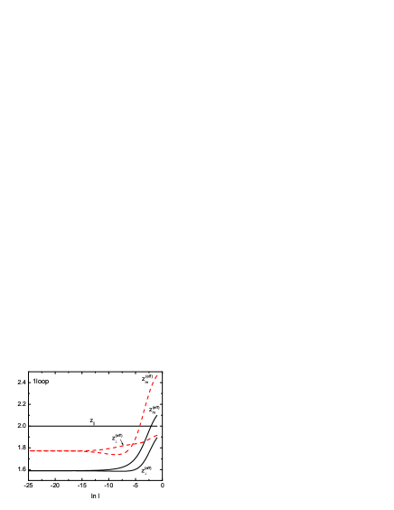
Figure 1: Effective dynamic exponents at $d=3$ calculated in one loop order using the one loop expression for the flow equations (64), (66). The effective exponents are calculated at the biconical FP (full lines) and at the Heisenberg FP (dashed line). $z_{\|}$ is valid for both FPs.

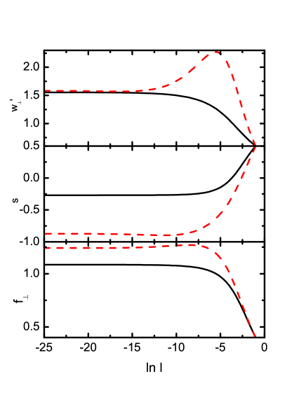
Figure 2: Flow of the parameters $w_{\perp}^{\prime}$, $s=w_{\perp}^{\prime\prime}/w_{\perp}^{\prime}$ and $f_{\perp}$ in one loop order at $d=3$. The calculation has been performed for the biconical (solid lines) and the Heisenberg (dashed lines) FP.

Inserting the FP value of the static $\zeta$-function $\zeta_{m}^{\star}$ (see relation (105) in paper III)

$$\zeta_{m}^{\star}=\frac{\phi}{\nu}-\frac{d}{2}$$ (95)

into the above equation one has

$$\zeta_{\Gamma_{\perp}}^{\prime\star}=\zeta_{\lambda}^{\star}=\frac{\phi}{\nu}-2\,.$$ (96)

The dynamic critical exponents (54) in one loop order are therefore completely expressed in terms of the static exponents:

$$z_{\perp}\equiv z_{\phi_{\perp}}=z_{m}=\frac{\phi}{\nu}\ ,\quad z_{\|}\equiv z_{\phi_{\|}}=2\,.$$ (97)

These static exponents might also be taken from static experiments. All our numerical calculations are performed in $d=3$ ($\epsilon=1$). The numerical values of the static exponents $\phi$ and $\nu$ have been calculated in two loop order in paper I and are given there in Tab.III ($\nu=\nu_{+}$ therein) in two loop order resummed. In one loop order the two OPs have different dynamic critical exponents. Scaling is fulfilled only between the perpendicular OP and the secondary density. The parallel OP behaves like the van Hove model. This is demonstrated in Fig.1, where the effective exponents defined in (55) - (57) have been calculated by using the flow equations in one loop order. At a flow parameter about $l\sim e^{-15}$ for both, the biconical FP (solid lines) and the Heisenberg FP (dashed lines), the asymptotic values of the dynamic exponents $z_{\perp}$ and $z_{m}$ are reached. The classical value $z_{\|}=2$, valid for both static fixed points, also is indicated by a straight line. The corresponding flow is presented in Fig.2, which proofs that the dynamic exponents in Fig.1 have reached their asymptotic behavior because the dynamic parameters are at their FP values at $\ln l=-25$.

FP	$u_{\|}^{\star}$	$u_{\perp}^{\star}$	$u_{\times}^{\star}$	$\gamma_{\|}^{\star}$	$\gamma_{\perp}\star$	$w^{\prime\star}_{\perp}$	$w^{\prime\prime\star}_{\perp}$	$f_{\perp}^{\star}$
${\mathcal{B}}$	1.28745	1.12769	0.30129	0.54201	-0.17806	1.55489	$\mp$ 0.41958	$\pm$ 1.08563
${\mathcal{B}}$	1.28745	1.12769	0.30129	-0.54201	0.17806	1.55489	$\pm$ 0.41958	$\pm$ 1.08563
${\mathcal{H}}$	1.00156	1.00156	1.00156	0.85179	-0.42590	1.58136	$\mp$ 1.38256	$\pm$ 1.24264
${\mathcal{H}}$	1.00156	1.00156	1.00156	-0.85179	0.42590	1.58136	$\pm$ 1.38256	$\pm$ 1.24264

Table 2: FP values of couplings and timescale ratios for $n_{\|}=1$, $n_{\perp}=2$ at $d=3$. ${\mathcal{B}}$ indicates the biconical, ${\mathcal{H}}$ the Heisenberg FP. There are always two equivalent static FPs depending on the signs of the couplings $\gamma$. The FP values of the static couplings $\{u\}$ and $\{\gamma\}$ are taken from the resummed two-loop results partI , whereas $w^{\star}_{\perp}$ and $f_{\perp}^{\star}$ are calculated from the one-loop $\beta$-functions. $w^{\star}_{\|}=v^{\star}=0$ is valid in all cases. Corresponding to the two equivalent cases in statics and the sign of $w^{\prime\prime\star}_{\perp}$ there are equivalent dynamic FPs with corresponding signs of the FP value of the mode coupling $f_{\perp}^{\star}$.

VIII Limiting behavior of the dynamical $\zeta$-functions in 2-loop order

The appearance of $\ln v$-terms in the two loop contribution to the $\zeta_{\Gamma_{\perp}}$-function, Eq (VI.1), changes the discussion of the fixed points considerably compared to the one loop case. In order to determine the dynamical fixed points of the current model in two loop order it is necessary to know something about the limiting behavior of the $\zeta$-functions. For this reason we will present the $\zeta$-functions in cases where one or several dynamical parameters go to zero or infinity under definite conditions. This is necessary because some $\zeta$-functions exhibit singular behavior under these conditions, which influences the discussion of possible fixed points. It is anticipated that the critical exponents defined by the values of the $\zeta$-functions at the FP are finite and real.

The auxiliary functions $X_{\perp}$, $L_{\perp}^{(\times)}$, $T_{1}$, $T_{2}$ and $L_{\|}^{(\times)}$, which appear in the $\zeta$-functions (VI.1) and (VI.1) behave singularly in several limits of the parameters. Thus several FP values of the different parameters can be excluded due to diverging $\zeta$-functions. For a summary of the subsequent analysis of the $\zeta$-function on the time scale ratios see Tab. 3.

i) At first we will consider the two functions $X_{\perp}$ and $L_{\perp}^{(\times)}$ in (74) and (79), which appear in $\zeta_{\Gamma_{\perp}}$ and depend on $v$ only. These two functions remain regular if $v$ grows to infinity. In this case one simply has $X_{\perp}(v\to\infty)=1$ and $L_{\perp}^{(\times)}(v\to\infty)=0$. But for vanishing $v$ both functions evolve a term proportional to $\ln v$. One gets

$$X_{\perp}(v\to 0)=\ln(2v)\,,\qquad L_{\perp}^{(\times)}(v\to 0)=1-\ln(2v)\,.$$ (98)

Thus divergent $\ln v$ terms appear in $\zeta_{\Gamma_{\perp}}(v\to 0)$ independent from the individual behavior of $w_{\perp}$ and $w_{\|}$ because only the ratio $v$ enters the function.

ii) The dynamic $\zeta$-function (VI.1) of the parallel component contains the three functions $T_{1}$, $T_{2}$ and $L_{\|}^{(\times)}$ defined in (81), (82) and (VI.1) which contain the ratio $v$. These functions, and therefore also $\zeta_{\Gamma_{\|}}$, remain non-divergent for vanishing $v$. One obtains

$$T_{1}(v\to 0)\!\!\! = \!\!\!D_{\perp}\left(1+\ln\left(1+\frac{1}{v_{\perp}}\right)-\frac{1}{v_{\perp}}\ln(1+v_{\perp})\right)\,,$$

$$T_{2}(v\to 0)\!\!\! = \!\!\!-w_{\perp}^{\star}D_{\perp}\left(\ln\left(1+\frac{1}{v_{\perp}}\right)+\ln(1+v_{\perp})\right)\,,$$

$$L_{\|}^{(\times)}(v\to 0)\!\!\! = \!\!\!0\,.$$ (99)

But they diverge when $v$ is growing to infinity:

$$T_{1}(v\to\infty)\!\!\! = \!\!\!D_{\perp}\ln\frac{\left(1+\frac{1}{v_{\perp}}\right)}{v}\,,$$

$$T_{2}(v\to\infty)\!\!\! = \!\!\!-w_{\perp}^{\star}D_{\perp}\ln\frac{\left(1+\frac{1}{v_{\perp}}\right)}{v}\,,$$

$$L_{\|}^{(\times)}(v\to\infty)\!\!\! = \!\!\!1+\ln\frac{v}{\left(1+\frac{1}{v_{\perp}}\right)}\,.$$ (100)

In contrast to the case i) the function $\zeta_{\Gamma_{\|}}$ in the parallel subspace evolves logarithmic terms $\ln v$ in the limit $v\to\infty$ and stays finite in the limit $v\to 0$. The above discussion is also independent of the individual behavior of $w_{\perp}$ and $w_{\|}$ because only the ratio $v_{\perp}$ stays always finite and the three functions $T_{1}$, $T_{2}$ and $L_{\|}^{(\times)}$ remain finite even for diverging time scale ratios if their prefactors are taken into account.

Limit	$\zeta_{\Gamma_{\perp}}$	$\zeta_{\Gamma_{\|}}$	$\zeta_{\lambda}$
$v\to 0$	$\sim\ln v$	regular	unaffected
$v\to\infty$	regular	$\sim\ln v$	unaffected
$w_{\perp}\to\infty$	$\sim\ln w_{\perp}$	regular	$\sim w_{\perp}^{\prime 2}$
$w_{\|}\to\infty$	regular	$\sim\ln w_{\|}$	unaffected
$w_{\perp}\to 0$	regular	$\sim\ln v$	regular
$w_{\|}\to 0$	$\sim\ln v$	regular	unaffected

Table 3: Limiting behavior of the dynamic $\zeta$-functions

iii) Additional logarithmic singularities may arise in the dynamic $\zeta$-functions if the time scale ratios $w_{\perp}$ and $w_{\|}$ grow individually to infinity independent of the behavior of $v$. A closer examination of (VI.1) reveals that in the limit $w_{\perp}\to\infty$ the $\zeta$-function is proportional to

$$\zeta_{\Gamma_{\perp}}(w_{\perp}\to\infty)\sim\frac{1}{2}\gamma_{\perp}^{4}\ln\frac{w_{\perp}}{2}$$ (101)

independent of the behavior of $v$. Quite analogously the same happens in (VI.1) when $w_{\|}$ grows to infinity. One obtains

$$\zeta_{\Gamma_{\|}}(w_{\|}\to\infty)\sim\frac{1}{2}\gamma_{\|}^{4}\ln\frac{w_{\|}}{2}\,.$$ (102)

Supposing a finite (different from zero or infinity) FP value $f_{\perp}^{\star}$ for the mode coupling parameter we may conclude the following concerning the allowed FP values of the remaining parameters:

a) From i) and ii) follows that $v^{\star}$ has to be also different from zero or infinity, otherwise $\ln v$ contributions would lead to divergent $\zeta$-functions.

b) From iii) follows that the finite $v^{\star}$ only can be realized either by $w_{\|}$ and $w_{\perp}$ both finite, or $w_{\|}$ and $w_{\perp}$ both going to zero in the same way. The possibility that both time scale ratios are going to infinity in the same way is excluded because of the $\ln w_{\|}$ and $\ln w_{\perp}$ terms appearing in this case.

IX General asymptotic relations

The FP values $\{\alpha_{j}^{\star}\}$ of the model parameters are found from the zeros of the $\beta$-functions in Eqs.(64)-(66). From the right hand side of the equations one obtains

$$w_{\perp}^{\star}\left(\zeta_{\Gamma_{\perp}}^{\star}-\zeta_{\lambda}^{\star}\right) = 0\ ,$$ (103)

$$w_{\|}^{\star}\left(\zeta_{\Gamma_{\|}}^{\star}-\zeta_{\lambda}^{\star}\right) = 0\ ,$$ (104)

$$f_{\perp}^{\star}\left(\varepsilon+\zeta_{\lambda}^{\star}-2\zeta_{m}^{\star}+\Re\left[\frac{w_{\perp}^{\star}}{w_{\perp}^{\prime^{\star}}}\ \zeta_{\Gamma_{\perp}}^{\star}\right]\right) = 0\ .$$ (105)

A FP which fulfills Eqs.(103)-(105) has to be also a solution of

$$v^{\star}\left(\zeta_{\Gamma_{\|}}^{\star}-\zeta_{\Gamma_{\perp}}^{\star}\right)=0$$ (106)

which follows from (67). The $\zeta$-function $\zeta_{\Gamma_{\perp}}$ for the perpendicular component of the OP relaxation is a complex function. Separating real and imaginary part leads to

$$\zeta_{\Gamma_{\perp}}=\zeta^{\prime}_{\Gamma_{\perp}}+i\zeta^{\prime\prime}_{\Gamma_{\perp}}\,.$$ (107)

As a consequence also the equations (103) for $w_{\perp}$ and (106) for $v$ are complex expressions. The $\zeta$-function for $\Gamma_{\perp}^{\prime}$ is

$$\zeta_{\Gamma_{\perp}^{\prime}}=\zeta^{\prime}_{\Gamma_{\perp}}-s\zeta^{\prime\prime}_{\Gamma_{\perp}}$$ (108)

with $s$ defined in (121).

We anticipate that in a real physical system definite dynamical exponents exist, and therefore the dynamic $\zeta$-functions have to be finite at the stable FP. As already mentioned in subsection VIII, the $\zeta$-functions contain $\ln v$ terms requiring a finite FP value $v^{\star}$ in order to obtain finite dynamical exponents. Separating (106) into real and imaginary part one has

$$v^{\prime\star}(\zeta^{\prime\star}_{\Gamma_{\perp}}-\zeta^{\star}_{\Gamma_{\|}})-v^{\prime\prime\star}\zeta^{\prime\prime\star}_{\Gamma_{\perp}}=0\,,$$ (109)

$$v^{\prime\star}\zeta^{\prime\prime\star}_{\Gamma_{\perp}}+v^{\prime\prime\star}(\zeta^{\prime\star}_{\Gamma_{\perp}}-\zeta^{\star}_{\Gamma_{\|}})=0\,.$$ (110)

From these two equations the FP relations

$$\zeta_{\Gamma_{\perp}}^{\prime\star}=\zeta_{\Gamma_{\|}}^{\star}\ ,\qquad\zeta_{\Gamma_{\perp}}^{\prime\prime\star}=0$$ (111)

immediately follow. The second equation in (111) implies that the dynamical exponent $z_{\phi_{\perp}}$ in (54) can be written as

$$z_{\phi_{\perp}}=2+\zeta_{\Gamma_{\perp}}^{\prime\star}\,.$$ (112)

From the first relation in (111) follows

$$z_{\phi_{\perp}}=z_{\phi_{\|}}\ .$$ (113)

This means that in the case of a finite FP value $v^{\star}$ scaling between the OPs is valid. In order to obtain a critical behavior different from model C, the FP value $f_{\perp}^{\star}$ of the mode coupling parameter also has to be finite and different from zero. Then from Eq.(105) follows

$$\varepsilon+\zeta_{\Gamma_{\perp}}^{\prime\star}+\zeta_{\lambda}^{\star}-2\zeta_{m}^{\star}=0\,,$$ (114)

where the second relation of (111) already has been used. Inserting (85) and (95) into (114) one obtains the relation

$$z_{\phi_{\perp}}+z_{m}=2\frac{\phi}{\nu}$$ (115)

between the exponents. In summary, the condition that both $v^{\star}$ and $f_{\perp}^{\star}$ have to be finite leads to the two relations (113) and (115) between the exponents. Further relations are dependent whether the FP values of the time scale ratios $w_{\perp}$ and $w_{\|}$ are finite or zero and lead to the following cases.

• Dynamical strong scaling FP:

  In the case that $w_{\perp}$ and $w_{\|}$ are finite at the FP, from (103) and (104) the relation

  $$\zeta_{\Gamma_{\perp}}^{\prime\star}=\zeta_{\Gamma_{\|}}^{\star}=\zeta_{\lambda}^{\star}$$ (116)

  is obtained, where (111) already has been used. From (54) it follows immediately that the dynamical exponents have to fulfill the relations

  $$z_{\phi_{\perp}}=z_{\phi_{\|}}=z_{m}\equiv z\,.$$ (117)

  Thus in the case of strong scaling one dynamical exponent $z$ exists only. The exact value of this exponent can be found by inserting (117) into (115). One obtains

  $$z=\frac{\phi}{\nu}\,.$$ (118)

• Dynamical weak scaling FP:

  In the case that $w_{\perp}$ and $w_{\|}$ are zero with $v$ finite at the FP, Eqs.(103) and (104) are trivially fulfilled and no additional relation between the $\zeta$-functions, and dynamical exponents respectively, arises. As a consequence two dynamical exponents exist. The first one

  $$z_{\phi_{\|}}=z_{\phi_{\perp}}=z_{OP}$$ (119)

  for the OPs, follows from relation (113). The second one

  $$z_{m}=2\frac{\phi}{\nu}-z_{OP}$$ (120)

  for the secondary density, is obtained from (115).

A closer examination of the $\beta$-functions (103) - (105), also with numerical methods in $d=3$, reveals that no FP solution can be found where both, $w_{\perp}$ and $w_{\|}$, are finite. Thus the only solution in $d=3$ which remains is $w_{\perp}^{\prime\star}=w_{\perp}^{\prime\prime\star}=w_{\|}^{\star}=0$ with $v^{\star}$ and $v_{\perp}^{\star}$ finite. This result of course depends also on the specific numerical values notefp of the static FPs (given in Tab 2) used in the dynamical equations. The stable FP lies then in the subspace where the time scale ratios $w_{\|}$ and $w_{\perp}$ approach zero in such a way that their ratios $v$ and $v_{\perp}$ remain finite and in general complex quantities. In order to obtain the finite FP values for $v$ and $v_{\perp}$ the two loop $\zeta$-functions may be reduced by setting $w_{\perp}$ and $w_{\|}$ equal to zero by keeping their ratios finite. This will be performed in the following section.

X Critical behavior in the asymptotic subspace

Since the asymmetric couplings $\gamma_{\alpha}$ always appear together with the time scale ratios $w_{\alpha}$ all terms proportional to these couplings drop out in the asymptotic limit where $w_{\alpha}\to 0$. It is convenient to introduce the real ratios

$$s\equiv\frac{w_{\perp}^{\prime\prime}}{w_{\perp}^{\prime}}=\frac{\Gamma_{\perp}^{\prime\prime}}{\Gamma_{\perp}^{\prime}}\ ,\qquad q\equiv\frac{w_{\|}}{w_{\perp}^{\prime}}=\frac{\Gamma_{\|}}{\Gamma_{\perp}^{\prime}}\,.$$ (121)

Thus only $s$, $q$ and $f_{\perp}$ remain as independent dynamical variables.

The ratio $s$ determines the behavior of the imaginary part of $w_{\perp}$ with respect to the real part, while the ratio $q$ indicates the behavior of $w_{\|}$ with respect to the real part of $w_{\perp}$. The complex parameters $v_{\perp}$ and $v$, introduced in (61) and (60), are expressed by $s$ and $q$ as

$$v_{\perp}=\frac{1+is}{1-is}\ ,\qquad v=\frac{q}{1+is}$$ (122)

in the following expressions.

X.1 $\zeta$-functions

We discuss the behavior of the $\zeta$-functions in the limit $w_{\perp}\to 0$ and $w_{\|}\to 0$ for $s$ and $q$ constant.

Case $s\neq 0:$

For $w_{\perp}=0$ and $w_{\|}=0$ the $\zeta$-function (VI.1), reduces to

$$\zeta_{\Gamma_{\perp}}^{(as)}\big{(}\{u\},s,q,f_{\perp}\big{)}=-\frac{f_{\perp}^{2}}{1+is}\Bigg{\{}1+\frac{2}{3}u_{\perp}\Big{(}L_{0}(s)$$

$$+x_{-}(s)x_{1}(s)L_{1}(s)\Big{)}-\frac{1}{2}\frac{f_{\perp}^{2}}{1+is}\Big{(}2x_{-}(s)L_{1}(s)$$

$$-2L_{0}(s)+L_{R}(s)\Big{)}\Bigg{\}}+\zeta_{\Gamma_{\perp}}^{(A)}\big{(}\{u\},s,q\big{)}\,.$$ (123)

The functions $x_{-}(s)$, $x_{1}(s)$, $L_{0}(s)$, $L_{1}(s)$ and $L_{R}(s)$ are the same as in (75) - (77) with $v_{\perp}$ replaced by (122). The same is true for $\zeta_{\Gamma_{\perp}}^{(A)}\big{(}\{u\},s,q\big{)}$, which has been defined in (VI.1), and where also (122) has been used to replace $v_{\perp}$ and $v$.

Performing the limit in the dynamical $\zeta$-function (VI.1) it reduces to

$$\zeta_{\Gamma_{\|}}^{(as)}\big{(}\{u\},s,q\big{)}=\zeta_{\Gamma_{\|}}^{(A)}\big{(}\{u\},s,q\big{)}$$ (124)

where $\zeta_{\Gamma_{\|}}^{(A)}\big{(}\{u\},s,q\big{)}$ is the model A function (VI.1) with relation (122) inserted into (VI.1).

Finally the function $X_{2}$ in (VI.2) simplifies for vanishing time scale ratios to

$$X_{2}^{(as)}\big{(}f_{\perp}\big{)}=\frac{f_{\perp}^{2}}{2}\,.$$ (125)

Inserting this expression into (88) and (87), the dynamical $\zeta$-function (85) reads

$$\zeta_{\lambda}^{(as)}\big{(}\{\gamma\},f_{\perp}\big{)}=\gamma_{\perp}^{2}+\frac{1}{2}\gamma_{\|}^{2}-\frac{f_{\perp}^{2}}{2}\left(1+\frac{f_{\perp}^{2}}{4}\right)\,.$$ (126)

The value of $v_{\perp}$ at the FP depends on how $w_{\perp}^{\prime}$ goes to zero in the critical limit $l\to 0$ compared to $w_{\perp}^{\prime\prime}$. There are three possible scenarios:

i) $w_{\perp}^{\prime\prime}$ goes to zero faster than $w_{\perp}^{\prime}$ so that $s\to 0$. Then $v_{\perp}$ is turning to the real value $1$.

ii) $w_{\perp}^{\prime}$ and $w_{\perp}^{\prime\prime}$ behave in the same way so that the ratio $s=s_{0}$ is constant. $v_{\perp}$ is in this case a complex constant

$$v_{\perp}=\frac{1+is_{0}}{1-is_{0}}\,.$$ (127)

iii) $w_{\perp}^{\prime}$ goes to zero faster than $w_{\perp}^{\prime\prime}$ so that $s\to\infty$. Then $v_{\perp}$ is turning to the real value $-1$.

The third of the three scenarios above can be excluded from the discussion because some of the $\zeta$-functions do not stay finite for $v_{\perp}=-1$. Finite $\zeta$-functions at the FP and therefore well defined critical exponents may be obtained only in the first two scenarios.

The $\zeta$-function for scenario ii) are already given in (X.1) - (126) when (127) is inserted.

Case $s=0:$

For $v_{\perp}=1$ ($s=0$) the $\zeta$-functions (X.1) and (124) simplify to

$$\zeta_{\Gamma_{\perp}}^{(as0)}\big{(}\{u\},q,f_{\perp}\big{)}=-f_{\perp}^{2}\Bigg{\{}1-\frac{f_{\perp}^{2}}{2}\Big{(}\frac{27}{2}\ln\frac{4}{3}-3\Big{)}\Bigg{\}}$$

$$+\zeta_{\Gamma_{\perp}}^{(A0)}\big{(}\{u\},q\big{)}\,,$$ (128)

$$\zeta_{\Gamma_{\|}}^{(as0)}\big{(}\{u\},q\big{)}=\zeta_{\Gamma_{\|}}^{(A0)}\big{(}\{u\},q\big{)}\,.$$ (129)

The model A functions (VI.1) and (VI.1) are now

$$\zeta_{\Gamma_{\perp}}^{(A0)}\big{(}\{u\},q\big{)}=\frac{u_{\perp}^{2}}{9}\left(3\ln\frac{4}{3}-\frac{1}{2}\right)$$

$$+\frac{u_{\times}^{2}}{36}\left(L_{\perp}^{(\times)}(q)-\frac{1}{2}\right)$$ (130)

and

$$\zeta_{\Gamma_{\|}}^{(A0)}\big{(}\{u\},q\big{)}=\frac{u_{\|}^{2}}{4}\left(\ln\frac{4}{3}-\frac{1}{6}\right)$$

$$+\frac{u_{\times}^{2}}{18}\left(L_{\|}^{(\times)}(q)-\frac{1}{2}\right)\,,$$ (131)

where in $L_{i}^{(\times)}(q)$, introduced in (79) and (VI.1), the relations (122) with $s=0$ have been inserted.

X.2 Fixed points in the asymptotic subspace

Inserting the $\zeta$-functions of the previous subsection into (103) - (105) one obtains the FP values in the asymptotic subspace for $s^{\star}$ finite, or $s^{\star}=0$. The results are presented in Tab.4 for the biconical (${\cal B}$) and the Heisenberg (${\cal H}$) FP. It turns out that especially at the biconical FP the values of the ratio $q$ are extremely small, but definitely not zero. Thus the asymptotic critical behavior in two loop order changes considerably compared to one loop (see section VII). Weak scaling as discussed in section IX is valid. The two order parameters scale with the same dynamic exponent $z_{OP}$ from relation (119), while the secondary density scales with a different dynamic exponent $z_{m}$ given in (120). The numerical values of these two dynamic exponents are also given in Tab.4 in two loop order. Note that the values of the dynamical exponents to the accuracy shown are independent wether the FP value of $s$ is zero or not.

	$f_{\perp}^{\star}$	$q^{\star}$	$s^{\star}$	$z_{OP}$	$z_{m}$
C C	-	-	$0$	$2.18$	$2.18$
F F	$0.83$	-	$0$	$\sim 1.5$	$\sim 1.5$
${\cal B}$	$1.232$	$1.167\cdot 10^{-86}$	$0$	$2.048$	$1.131$
${\cal H}$	$1.211$	$3.324\cdot 10^{-8}$	$0$	$2.003$	$1.542$
${\cal B}$	$1.232$	$2.51\cdot 10^{-782}$	$0.705$	$2.048$	$1.131$
${\cal H}$	$1.211$	$3.16\cdot 10^{-66}$	$0.698$	$2.003$	$1.542$

Table 4: FP values of the mode coupling $f_{\perp}$ and the ratios $q=w_{\|}/w_{\perp}^{\prime}$ and $s=w_{\perp}^{\prime\prime}/w_{\perp}^{\prime}$ in the subspace $w_{\|}=0$, $w_{\perp}=0$ and finite $v=q/(1+is)$ for different cases of the biconical ${\mathcal{B}}$ and Heisenberg ${\mathcal{H}}$ FP in $d=3$. For comparison results for model C and model F FPs are shown at $n=1$ and $n=2$, correspondingly.

The comparison with the dynamical critical exponents in the cases when the OPs decouple statically and dynamically into model C and model F shows the changes in the multicritical case where the exponents are changed but each component reflects the decoupled values accordingly.

X.3 Effective exponents in the asymptotic subspace

The flow of the parameters $q$, $s$ and $f_{\perp}$ can be found by solving the equations

$$l\frac{dq}{dl} = q\left(\zeta_{\Gamma_{\|}}^{(as)}-\Re[\zeta_{\Gamma_{\perp}}^{(as)}]+s\Im[\zeta_{\Gamma_{\perp}}^{(as)}]\right)\ ,$$ (132)

$$l\frac{ds}{dl} = (1+s^{2})\Im[\zeta_{\Gamma_{\perp}}^{(as)}]\ ,$$ (133)

$$l\frac{df_{\perp}}{dl} = -\frac{f_{\perp}}{2}\Big{(}\varepsilon+\zeta_{\lambda}^{(as)}-2\zeta_{m}+\Re[\zeta_{\Gamma_{\perp}}^{(as)}]$$ (134)

$$-s\Im[\zeta_{\Gamma_{\perp}}^{(as)}]\Big{)}.$$

Figure 3: Effective dynamic exponents in the subspace $w_{\|}=w_{\perp}=0$ with $q$ and $s$ finite in $d=3$. The static values are taken for the Heisenberg FP and for the biconical FP. The non-asymptotic region is extended by a factor 10 at the biconical FP. For the static FP values see Tab. 2, for the dynamic FP values Tab. 4.

The $\zeta$-functions in the above flow equations are the reduced expressions (X.1), (124) and (126), which are functions of $q,s,f_{\perp}$. We consider the case $s\neq 0$ since the FP $s^{\star}=0$ is reached only starting with $s=0$. From the solution of Eqs.(133)-(134) the flow $q(l)$, $s(l)$, $f_{\perp}(l)$ is obtained, which is used to calculate asymptotic effective dynamic exponents

$$z_{\perp}^{(as)}(l) = 2+\Re\big{[}\zeta_{\Gamma_{\perp}}^{(as)}\big{(}q(l),s(l),f_{\perp}(l)\big{)}\big{]}$$ (135)

$$-s(l)\Im\big{[}\zeta_{\Gamma_{\perp}}^{(as)}\big{(}q(l),s(l),f_{\perp}(l)\big{)}\big{]}\ ,$$

$$z_{\|}^{(as)}(l) = 2+\zeta_{\Gamma_{\|}}^{(as)}\big{(}q(l),s(l)\big{)}\ ,$$ (136)

$$z_{m}^{(as)}(l) = 2+\zeta_{\lambda}^{(as)}\big{(}q(l),s(l),f_{\perp}(l)\big{)}\ .$$ (137)

They can be calculated for different static fixed points, i.e. biconical or Heisenberg FP, as presented in Fig.3. The values of $u_{\perp}^{\star}$, $u_{\|}^{\star}$, $u_{\times}^{\star}$, as well as $\gamma_{\perp}^{\star}$, $\gamma_{\|}^{\star}$, used in the current calculations can be found in Tab.II. At both fixed points weak scaling, as discussed in section IX, is fulfilled. The difference to the one loop result is now that the dynamic exponents $z_{\perp}$ and $z_{\|}$ of the OPs are equal in the asymptotic region, while $z_{m}$ stays different. Moreover the transient exponents in two loop order are very small compared to one loop. There the effective exponents reach their asymptotic values about $l\sim e^{-15}$ as can be seen from Fig.1. In two loop order the asymptotic region is of magnitudes smaller. From Fig.3 one can see that at the Heisenberg FP the flow parameter has to be of the order $l\sim e^{-1500}$ to obtain the asymptotic values of the dynamic exponents. At the biconical FP $l$ has to be even of the order $l\sim e^{-15000}$ (note that there is a factor $10$ between the $x$-scales in Fig.3) to reach asymptotic values. However as will be seen in the next section the subspace will not be reached by the flow in the complete parameter space for reasonable values of $l$.

XI General flow and pseudo-asymptotics

Although in general the dynamic flow equations have to be solved in the full parameter space, the results for the effective exponents presented in the previous subsection are obtained from the flow equations which already have been reduced to the subspace $w_{\perp}=w_{\|}=0$. The reason to do this is that the flow and the $\zeta$-functions in the full parameter space shows some peculiar behavior.

In the non-asymptotic region the flow is generated by the system of equations for four parameters which are $w_{\perp}^{\prime}$, $s$, $w_{\|}$ and $f_{\perp}$ obtained from Eqs. (64) - (66) and (121). The static parameters are taken at their FP values given in Tab. 2. Due to the presence of the static asymmetric couplings $\gamma_{i}$ and the mode coupling $f_{\perp}$ an imaginary part of $w_{\perp}$ is produced even if one starts with a zero initial value.

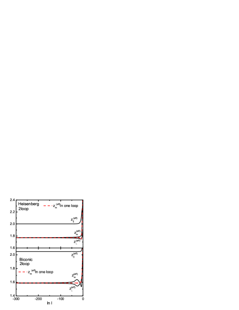
Figure 4: Effective dynamic exponents in the background using the flow equations (64), (66) in two loop order in $d=3$ in the complete dynamical parameter space (full lines). For comparison the effective dynamic exponent $z_{m}^{(eff)}$ in one loop order is shown (dashed line).

Starting with a typical set of initial values, i.e. $w_{\|}(l_{0})=0.3$, $w_{\perp}^{\prime}(l_{0})=0.6$, $s(l_{0})=0.5$ and $f_{\perp}(l_{0})=0.4$ at the flow parameter value $\ln l_{0}=-1$, the effective exponents in the complete parameter space have been calculated in $d=3$. The result is presented in Fig.4 for both static fixed points, where the solid lines are the results of the two loop calculation and the dashed line is a result of a complete (flow and effective exponent) one loop calculation. However the static FP values from Tab. 2 have been used also in the dynamic one loop flow. There it seems that in two loop order the same results as in the one loop calculation are obtained. $z_{\perp}^{eff}$ and $z_{m}^{eff}$ are getting close together (solid lines) for flow parameters $l<e^{-100}$ and seem to coincide even numerically with the corresponding results in one loop order (dashed line). This is the type of weak scaling in one loop order, which also can be seen from Fig.1 and in qualitative contradiction to the discussion in the previous sections (see Fig.3). But the examination of the flow of the dynamic parameters reveals a fundamental difference between the one and two loop calculation. In one loop order the dynamic parameters $w_{\perp}^{\prime}$, $s$, $w_{\|}$ and $f_{\perp}$ merge to the FP values when the effective exponents turns over in their constant asymptotic values, which is presented in Fig.2. This happens in the region about $l<e^{-15}$ and the dynamic parameters stay constant for all lower flow parameter values. In two loop order the situation is different. Although the two loop results for the effective exponents look like one has reached the asymptotic region (the exponents seem to be constant), the dynamic parameters in contrast are far from their asymptotic FP values. This is presented in Fig.5. The parameters $w_{\perp}^{\prime}$ and $s$ are still increasing and obviously have not reached a FP value. At the first glance the flow of $f_{\perp}$ seems to have reached a FP value (see lowest plot in Fig.5). But a closer examination shows that this is not the case. $f_{\perp}$ is constantly increasing with a very small slope as can be seen from the inserted small figure, where both axes has been enlarged. Actually the set of two loop $\beta$-functions does not have a zero for finite $w_{\perp}$ and $w_{\|}$, and therefore no FP exists in the parameter region of Fig.5.

Figure 5: Flow of the parameters $w_{\perp}^{\prime}$, $s$ and $f_{\perp}$ in the full parameter space

Thus the effective exponents in two loop order in Fig.4 only show a pseudo-asymptotic behavior completely different from real asymptotic behavior (there $z_{\perp}^{eff}$ and $z_{\|}^{eff}$ have to be equal) discussed in section X.3 (see Fig. 3). Even if one draws the $x$-axis in Fig.4 down to $\ln l=-20000$, as done for the flow in Fig.5, the picture remains to be the same, that is the effective exponents seem to be constant, with the exception that the background behavior is not longer visible because the region is too small. Also if one changes initial conditions of the parameters the qualitative result remains the same. The different flows merge within a region of $\ln l=-150$ to the same result.

Figure 6: Relative slope of the parameters $w_{\perp}^{\prime}$ and $f_{\perp}$ in the full parameter space

In order to get some insight how this pseudo-asymptotic behavior is possible, in Fig.6 the relative slopes

$$\frac{1}{\alpha_{i}}\frac{d\alpha_{i}}{d\ln l}=\frac{\beta_{\alpha_{i}}}{\alpha_{i}}$$ (138)

for the parameters $\alpha_{i}$ chosen to be $w_{\perp}^{\prime}$ and $f_{\perp}$ have been calculated. One can see that the relative changes in these parameters drop down to very small values. As a first consequence one has to calculate down to extremely small flow parameter values $\ln l<-10^{8}$ where one can expect to leave the pseudo-asymptotic region. But although the $\beta$-functions cannot be zero in the considered parameter range they may reach values which are so small that they cannot longer be separated numerically from zero. This means that coming from the background it is impossible to pass the pseudo-asymptotic region numerically into the real asymptotic region. This is the reason why in the previous section the flow has been started in an asymptotic subspace.

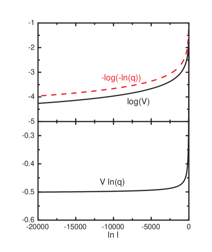
Figure 7: Contribution of the $V^{\prime}\ln q$ term in (140) (lower figure). It is of the same magnitude as the other terms in the $\zeta$-function. $V^{\prime}$ and $\ln q$ have the same behavior with opposite exponents. This is demonstrated in the upper figure, where the decadic logarithm of $V^{\prime}$ (solid curve) and the negative decadic logarithm of $-\ln q$ has been drawn (dashed curves).

Due to the presence of logarithmic terms in the timescale ratio $v$ the FP value of $v$ has to be finite. As follows from Tab. 4 via Eq. (122) it turns out to be very small leading to very large (negative) values of $\ln v$. So one expects that the $\ln v$-terms begin to dominate $\zeta_{\Gamma_{\perp}}$ in a certain region of $\ln l$ near the asymptotics. Making the $\ln v$-terms explicit one may rewrite $\zeta_{\Gamma_{\perp}}$, given in Eq. (VI.1), as

$$\zeta_{\Gamma_{\perp}}=-\frac{1}{2}\frac{\gamma_{\|}D_{\perp}}{1+w_{\perp}}\left(\frac{u_{\times}}{3}+\frac{1}{2}\frac{\gamma_{\|}D_{\perp}}{1+w_{\perp}}\right)\ln v$$

$$-\frac{u_{\times}^{2}}{36}\ln v+\mbox{remaining terms}\,.$$ (139)

Inserting Eq. (122), the essential term is the real part $V^{\prime}$ of the prefactor of $\ln q$. One obtains

$$\zeta_{\Gamma_{\perp}}=V^{\prime}\ln q+\mbox{remaining terms}\,.$$ (140)

The prefactor $V^{\prime}$ is

$$V^{\prime}=-\left[\frac{u^{2}_{\times}}{36}+\frac{1}{2}\gamma_{\|}A\left(\frac{u_{\times}}{3}+\frac{1}{2}\gamma_{\|}A\right)-\frac{1}{4}\gamma^{2}_{\|}B^{2}\right]$$ (141)

with

$$A=\frac{w_{\perp}^{\prime}[(1+w_{\perp}^{\prime}+w_{\perp}^{\prime}s^{2})\gamma_{\perp}-sF]}{(1+w_{\perp}^{\prime})^{2}+(w_{\perp}^{\prime}s)^{2}}\,,$$ (142)

$$B=\frac{w_{\perp}^{\prime}s\gamma_{\perp}-(1+w_{\perp}^{\prime})F]}{(1+w_{\perp}^{\prime})^{2}+(w_{\perp}^{\prime}s)^{2}}\,.$$ (143)

In Fig.7 the behavior of the $\ln q$-contributions to $\zeta_{\Gamma_{\perp}}$ at the biconical FP is presented. Although the $\ln q$ term already reaches very large negative values ($q$ is very small), as expected, this is compensated by the prefactor $V^{\prime}$ which has very small values in the considered region. In the upper part of Fig.7 the decadic logarithm of $V^{\prime}$ and $-\ln q$ have been plotted. Both curves show a similar behavior and a small difference. In the lower part $V^{\prime}\ln q$ is calculated from (141) - (143). As a consequence of the results in the upper part of the figure the numerical values are about $-0.5$ and one can see that the term is far away from being the leading one. There are other contributions to $\zeta_{\Gamma_{\perp}}$ which have the same magnitude. Thus the $\zeta$-function is not in the asymptotic region as has been also indicated by the flow in Fig.5.

Thus one expects in the experimentally accessible region non-universal effective dynamical critical behavior. This is described in the crossover region to the background by the flow equations together with a suitable matching condition related to the temperature distance, the wave vector modulus etc. The initial conditions have to be found by comparison with experiment.

XII Conclusion

Our two loop calculation for the dynamics at the multicritical point in anisotropic antiferromagnets in an external magnetic field leads to a FP where the OPs characterizing the parallel and perpendicular ordering with respect to the external field scale in the same way (strong dynamic scaling). This holds independent wether the Heisenberg FP or the biconical FP in statics is the stable one. The non-asymptotic analysis of the dynamic flow equations show that due to cancelation effects the critical behavior is described - in distances from the critical point accessible to experiments - by the critical behavior qualitatively found in one loop order. That means the time scales of the two OP components become almost constant in a so called pseudo-asymptotic region and scale differently.

So far we have not included the non-asymptotic flow of the static parameters which are expected to lead to minor deviations from the overall picture. Another item would be the study of the decoupled FP since in the non-asymptotic region the OPs remain statically and dynamically coupled and the behavior depend on the stability exponents how fast these effects decay. This in turn depends on the distance of the system in dimensional space and the space of the OP components from the stability border line to other FPs than the decoupled FP (see Fig. 1 in paper I).

The numerical results presented in this series of papers have been calculated for dimension $d=3$. One might speculate that the peculiar behavior found is specific to the dimension of the physical space rather than to the multicritical character of the specific point. This aspect was out of the scope of this series of papers. We note that the two critical lines meet at the multicritical point (bicritical or tetracritical) tangential. This has been taken into account for the nonsaymptotic behavior by choosing a path approaching the multicritical point without meeting one of the two critical lines cond . The nonasymptotic behavior in fact is more complicated since two critical length scales are present in the system. This has to be taken into account when studying the crossover behavior in approaching one of the critical lines amit78 .

Only recently a bicritical point has been identified by computer simulation selke . The corresponding FP has been identified as the Heisenberg FP which corresponds to the type of phase diagram obtained. It seems to be difficult to look for situations where a phase diagram containing a tetracritical point is present. Even more complicated would it be to identify the dynamical characteristic of this multicritical point, where - coming from the disordered phase - two lines belonging to different dynamic universality classes meet. The dynamical universality class of the case with a $n=1$ OP (model C) has been studied in sen ; stauffer with different results leading to critical exponents larger than expected. The dynamical universality class of the case with a $n=2$ OP (model F) case has been studied by computer simulations in krech ; landau . The methods of these simulations might be extended in order to be used also in the case of the multicritical point studied in this paper.

Acknowledgment
This work was supported by the Fonds zur Förderung der wissenschaftlichen Forschung under Project No. P19583-N20.

Yu.H. acknowledges partial support from the FP7 EU IRSES project N269139 ’Dynamics and Cooperative Phenomena in Complex Physical and Biological Media’.

We thank one of the referees for the exceptionally critical and precise remarks which have improved the presentation.

Appendix A Calculation of the dynamic vertex functions of the OPs

In perturbation expansion up to two loop order the functions $\mathring{\Omega}_{\psi\tilde{\psi}^{+}}$, $\mathring{\Gamma}^{(d)}_{\psi\tilde{\psi}^{+}}$ and $\mathring{\Omega}_{\phi_{\|}\tilde{\phi}_{\|}}$, which appear in (27) and (28), can be written as

$$\mathring{\Omega}_{\psi\tilde{\psi}^{+}}(\xi_{\perp},\xi_{\|},k,\omega)=1+\mathring{\Omega}^{(1L)}_{\psi\tilde{\psi}^{+}}(\xi_{\perp},k,\omega)$$

$$+\mathring{\Omega}^{(2L)}_{\psi\tilde{\psi}^{+}}(\xi_{\perp},\xi_{\|},k,\omega)\,,$$ (144)

$$\mathring{\Gamma}^{(d)}_{\psi\tilde{\psi}^{+}}(\xi_{\perp},\xi_{\|},k,\omega)=2\Big{[}\mathring{\Gamma}_{\perp}+\mathring{G}^{(1L)}_{\psi\tilde{\psi}^{+}}(\xi_{\perp},k,\omega)$$

$$+\mathring{G}^{(2L)}_{\psi\tilde{\psi}^{+}}(\xi_{\perp},\xi_{\|},k,\omega)\Big{]}\,,$$ (145)

$$\mathring{\Omega}_{\phi_{\|}\tilde{\phi}_{\|}}(\xi_{\perp},\xi_{\|},k,\omega)=1+\mathring{\Omega}^{(1L)}_{\phi_{\|}\tilde{\phi}_{\|}}(\xi_{\|},k,\omega)$$

$$+\mathring{\Omega}^{(2L)}_{\phi_{\|}\tilde{\phi}_{\|}}(\xi_{\perp},\xi_{\|},k,\omega)\,.$$ (146)

The superscript $(iL)$ indicates the loop order. Of course all functions considered depend on all model parameters (couplings and kinetic coefficients), but only the independent lengths $\xi_{\perp}$, $\xi_{\|}$, $k$ and $\omega$ will be mentioned explicitly in the following. The one loop contributions are

$$\mathring{\Omega}^{(1L)}_{\psi\tilde{\psi}^{+}}(\xi_{\perp},k,\omega)=\big{(}\mathring{\Gamma}_{\perp}\mathring{\gamma}_{\perp}-\mbox{i}\mathring{g}\big{)}\mathring{\gamma}_{\perp}I_{\perp}(\xi_{\perp},k,\omega)\,,$$ (147)

$$\mathring{G}^{(1L)}_{\psi\tilde{\psi}^{+}}(\xi_{\perp},k,\omega)=\big{(}\mathring{\Gamma}_{\perp}\mathring{\gamma}_{\perp}-\mbox{i}\mathring{g}\big{)}\mbox{i}\mathring{g}I_{\perp}(\xi_{\|},k,\omega)\,,$$ (148)

$$\mathring{\Omega}^{(1L)}_{\phi_{\|}\tilde{\phi}_{\|}}(\xi_{\|},k,\omega)=\mathring{\Gamma}_{\|}\mathring{\gamma}_{\|}^{2}I_{\|}(\xi_{\|},k,\omega)\,.$$ (149)

The one loop integrals $I_{\perp}$ and $I_{\|}$ in (147)-(149) read

$$I_{\perp}(\xi_{\perp},k,\omega)=\int_{k^{\prime}}\frac{1}{\big{(}\xi_{\perp}^{-2}\!+\!(k\!+\!k^{\prime})^{2}\big{)}(-\mbox{i}\omega+\alpha_{\perp}^{\prime})}\,,$$ (150)

$$I_{\|}(\xi_{\|},k,\omega)=\int_{k^{\prime}}\frac{1}{\big{(}\xi_{\|}^{-2}\!+\!(k\!+\!k^{\prime})^{2}\big{)}(-\mbox{i}\omega+\alpha_{\|}^{\prime})}\,.$$ (151)

The dynamic propagators $\alpha_{\perp}^{\prime}$ and $\alpha_{\|}^{\prime}$ are defined as

$$\alpha_{\perp}^{\prime}\equiv\mathring{\Gamma}_{\perp}\big{(}\xi_{\perp}^{-2}\!+\!(k\!+\!k^{\prime})^{2}\big{)}+\mathring{\lambda}k^{\prime 2}\,,$$ (152)

$$\alpha_{\|}^{\prime}\equiv\mathring{\Gamma}_{\|}\big{(}\xi_{\|}^{-2}\!+\!(k\!+\!k^{\prime})^{2}\big{)}+\mathring{\lambda}k^{\prime 2}\,.$$ (153)

The two loop contributions to the dynamic vertex function of the orthogonal components (A) and (A) have the structure

$$\mathring{\Omega}^{(2L)}_{\psi\tilde{\psi}^{+}}(\xi_{\perp},\xi_{\|},k,\omega)=\frac{2}{9}\mathring{\Gamma}_{\perp}\mathring{u}_{\perp}^{2}\mathring{W}^{(A_{\perp})}_{\psi\tilde{\psi}^{+}}(\xi_{\perp},k,\omega)$$

$$+\frac{1}{18}\mathring{\Gamma}_{\perp}\mathring{u}_{\times}^{2}\mathring{W}^{(A_{\times})}_{\psi\tilde{\psi}^{+}}(\xi_{\perp},\xi_{\|},k,\omega)$$

$$-\frac{2}{3}\big{(}2\mathring{\Gamma}_{\perp}\mathring{\gamma}_{\perp}-\mbox{i}\mathring{g}\big{)}\mathring{u}_{\perp}\mathring{F}^{(T3_{\perp})}_{\psi\tilde{\psi}^{+}}(\xi_{\perp},k,\omega)$$

$$-\frac{1}{6}\big{(}2\mathring{\Gamma}_{\perp}\mathring{\gamma}_{\perp}-\mbox{i}\mathring{g}\big{)}\mathring{u}_{\times}\mathring{F}^{(T3_{\times})}_{\psi\tilde{\psi}^{+}}(\xi_{\perp},\xi_{\|},k,\omega)$$

$$+\big{(}\mathring{\Gamma}_{\perp}\mathring{\gamma}_{\perp}-\mbox{i}\mathring{g}\big{)}\mathring{\gamma}_{\perp}\mathring{F}_{\psi\tilde{\psi}^{+}}(\xi_{\perp},\xi_{\|},k,\omega)$$ (154)

and

$$\mathring{G}^{(2L)}_{\psi\tilde{\psi}^{+}}(\xi_{\perp},\xi_{\|},k,\omega)=-\frac{2}{3}\mathring{\Gamma}_{\perp}\mathring{u}_{\perp}\mbox{i}\mathring{g}\mathring{F}^{(T3_{\perp})}_{\psi\tilde{\psi}^{+}}(\xi_{\perp},k,\omega)$$

$$-\frac{1}{6}\mathring{\Gamma}_{\perp}\mathring{u}_{\times}\mbox{i}\mathring{g}\mathring{F}^{(T3_{\times})}_{\psi\tilde{\psi}^{+}}(\xi_{\perp},\xi_{\|},k,\omega)$$

$$+\big{(}\mathring{\Gamma}_{\perp}\mathring{\gamma}_{\perp}-\mbox{i}\mathring{g}\big{)}\mbox{i}\mathring{g}\mathring{F}_{\psi\tilde{\psi}^{+}}(\xi_{\perp},\xi_{\|},k,\omega)\,.$$ (155)

Note that both two loop functions differ only in terms containing the static fourth order couplings $\mathring{u}_{\perp}$ and $\mathring{u}_{\times}$. The remaining contributions are the same in both functions apart from a factor $\mathring{\gamma}_{\perp}$ and $i\mathring{g}$ respectively. The function $\mathring{F}_{\psi\tilde{\psi}^{+}}$ is defined as

$$\mathring{F}_{\psi\tilde{\psi}^{+}}(\xi_{\perp},\xi_{\|},k,\omega)\equiv\big{(}\mathring{\Gamma}_{\perp}\mathring{\gamma}_{\perp}-\mbox{i}\mathring{g}\big{)}^{2}\mathring{F}^{(T4_{\perp})}_{\psi\tilde{\psi}^{+}}(\xi_{\perp},k,\omega)$$

$$+\mathring{F}^{(T5_{\perp})}_{\psi\tilde{\psi}^{+}}(\xi_{\perp},k,\omega)-\mathring{\gamma}_{\perp}\mathring{F}^{(T3_{\perp})}_{\psi\tilde{\psi}^{+}}(\xi_{\perp},k,\omega)$$

$$+\frac{1}{2}\left(\mathring{F}^{(T5_{\times})}_{\psi\tilde{\psi}^{+}}(\xi_{\perp},\xi_{\|},k,\omega)-\mathring{\gamma}_{\|}\mathring{F}^{(T3_{\times})}_{\psi\tilde{\psi}^{+}}(\xi_{\perp},\xi_{\|},k,\omega)\right)$$

$$+\mathring{F}^{(T6_{\perp})}_{\psi\tilde{\psi}^{+}}(\xi_{\perp},k,\omega)-\mathring{\gamma}_{\perp}\mathring{F}^{(T3_{\perp})}_{\psi\tilde{\psi}^{+}}(\xi_{\perp},k,\omega)\,.$$ (156)

The first two loop contributions in (A) come from the bicritical model A. The integrals $\mathring{W}^{(A_{i})}_{\psi\tilde{\psi}^{+}}$ are defined by

$$\mathring{W}^{(A_{\perp})}_{\psi\tilde{\psi}^{+}}(\xi_{\perp},k,\omega)=\int_{k^{\prime}}\int_{k^{\prime\prime}}\frac{1}{\big{(}\xi_{\perp}^{-2}{+}(k{+}k^{\prime})^{2}\big{)}(\xi_{\perp}^{-2}{+}k^{\prime\prime 2})\big{(}\xi_{\perp}^{-2}{+}(k^{\prime}{+}k^{\prime\prime})^{2}\big{)}(-\mbox{i}\omega{+}A_{\perp\perp^{+}\perp})}\,,$$ (157)

$$\mathring{W}^{(A_{\times})}_{\psi\tilde{\psi}^{+}}(\xi_{\perp},\xi_{\|},k,\omega)=\int_{k^{\prime}}\int_{k^{\prime\prime}}\frac{1}{\big{(}\xi_{\perp}^{-2}{+}(k{+}k^{\prime})^{2}\big{)}(\xi_{\|}^{-2}{+}k^{\prime\prime 2})\big{(}\xi_{\|}^{-2}{+}(k^{\prime}{+}k^{\prime\prime})^{2}\big{)}(-\mbox{i}\omega{+}A_{\perp\|\|})}$$ (158)

with

$$A_{\perp\perp^{+}\perp}\equiv\mathring{\Gamma}_{\perp}\big{(}\xi_{\perp}^{-2}{+}(k{+}k^{\prime})^{2}\big{)}+\mathring{\Gamma}_{\perp}^{+}(\xi_{\perp}^{-2}{+}k^{\prime\prime 2})$$

$$+\mathring{\Gamma}_{\perp}\big{(}\xi_{\perp}^{-2}{+}(k^{\prime}{+}k^{\prime\prime})^{2}\big{)}$$ (159)

and

$$A_{\perp\|\|}\equiv\mathring{\Gamma}_{\perp}\big{(}\xi_{\perp}^{-2}{+}(k{+}k^{\prime})^{2}\big{)}+\mathring{\Gamma}_{\|}(\xi_{\|}^{-2}{+}k^{\prime\prime 2})$$

$$+\mathring{\Gamma}_{\|}\big{(}\xi_{\|}^{-2}{+}(k^{\prime}{+}k^{\prime\prime})^{2}\big{)}\,.$$ (160)

The further two loop contributions in (A)-(A) are marked with superscripts $(Ti)$, which indicate the different graph topologies. The explicit expressions are

$$\mathring{F}^{(T3_{\perp})}_{\psi\tilde{\psi}^{+}}(\xi_{\perp},k,\omega)=\int_{k^{\prime}}\int_{k^{\prime\prime}}\frac{1}{\big{(}\xi_{\perp}^{-2}{+}(k{+}k^{\prime})^{2}\big{)}(-\mbox{i}\omega{+}\alpha_{\perp}^{\prime})(-\mbox{i}\omega{+}A_{\perp\perp^{+}\perp})}\Bigg{(}\frac{\mathring{\Gamma}_{\perp}\mathring{\gamma}_{\perp}{-}\mbox{i}\mathring{g}}{\xi_{\perp}^{-2}{+}k^{\prime\prime 2}}+\frac{\mathring{\Gamma}_{\perp}^{+}\mathring{\gamma}_{\perp}{+}\mbox{i}\mathring{g}}{\xi_{\perp}^{-2}{+}(k^{\prime}{+}k^{\prime\prime})^{2}}\Bigg{)}\,,$$ (161)

$$\mathring{F}^{(T3_{\times})}_{\psi\tilde{\psi}^{+}}(\xi_{\perp},\xi_{\|},k,\omega)=\int_{k^{\prime}}\int_{k^{\prime\prime}}\frac{2\mathring{\Gamma}_{\|}\mathring{\gamma}_{\|}}{\big{(}\xi_{\perp}^{-2}{+}(k{+}k^{\prime})^{2}\big{)}(\xi_{\|}^{-2}{+}k^{\prime\prime 2})(-\mbox{i}\omega{+}\alpha_{\|}^{\prime})(-\mbox{i}\omega{+}A_{\perp\|\|})}\,,$$ (162)

$$\mathring{F}^{(T4_{\perp})}_{\psi\tilde{\psi}^{+}}(\xi_{\perp},k,\omega)=\int_{k^{\prime}}\int_{k^{\prime\prime}}\!\!\frac{1}{\big{(}\xi_{\perp}^{-2}\!+\!(k\!+\!k^{\prime}\!+\!k^{\prime\prime})^{2}\big{)}(-\mbox{i}\omega+\alpha_{\perp}^{\prime})^{2}(-\mbox{i}\omega+\beta_{\perp})}\,,$$ (163)

$$\mathring{F}^{(T5_{\perp})}_{\psi\tilde{\psi}^{+}}(\xi_{\perp},k,\omega)=\int_{k^{\prime}}\int_{k^{\prime\prime}}\frac{\mathring{\gamma}_{\perp}\mathring{\lambda}k^{\prime 2}{-}\mbox{i}\mathring{g}[(k^{\prime}{+}k^{\prime\prime})^{2}{-}k^{\prime\prime 2}]}{\big{(}\xi_{\perp}^{-2}{+}(k{+}k^{\prime})^{2}\big{)}(-\mbox{i}\omega{+}\alpha_{\perp}^{\prime})^{2}(-\mbox{i}\omega{+}A_{\perp\perp^{+}\perp})}\Bigg{(}\frac{\mathring{\Gamma}_{\perp}\mathring{\gamma}_{\perp}{-}\mbox{i}\mathring{g}}{\xi_{\perp}^{-2}{+}k^{\prime\prime 2}}+\frac{\mathring{\Gamma}_{\perp}^{+}\mathring{\gamma}_{\perp}{+}\mbox{i}\mathring{g}}{\xi_{\perp}^{-2}{+}(k^{\prime}{+}k^{\prime\prime})^{2}}\Bigg{)}\,,$$ (164)

$$\mathring{F}^{(T5_{\times})}_{\psi\tilde{\psi}^{+}}(\xi_{\perp},\xi_{\|},k,\omega)=\int_{k^{\prime}}\int_{k^{\prime\prime}}\frac{2\mathring{\Gamma}_{\|}\mathring{\gamma}_{\|}^{2}\mathring{\lambda}k^{\prime 2}}{\big{(}\xi_{\perp}^{-2}{+}(k{+}k^{\prime})^{2}\big{)}(\xi_{\|}^{-2}{+}k^{\prime\prime 2})(-\mbox{i}\omega{+}\alpha_{\perp}^{\prime})^{2}(-\mbox{i}\omega{+}A_{\perp\|\|})}\,,$$ (165)

$$\mathring{F}^{(T6_{\perp})}_{\psi\tilde{\psi}^{+}}(\xi_{\perp},k,\omega)=\!\!\!\!\! \!\!\!\!\!\int_{k^{\prime}}\int_{k^{\prime\prime}}\!\!\frac{\mathring{\gamma}_{\perp}\mathring{\lambda}k^{\prime\prime 2}{+}\mbox{i}\mathring{g}[(k{+}k^{\prime}{+}k^{\prime\prime})^{2}{-}(k{+}k^{\prime})^{2})]}{\big{(}\xi_{\perp}^{-2}{+}(k{+}k^{\prime})^{2}\big{)}(-\mbox{i}\omega{+}\alpha_{\perp}^{\prime})(-\mbox{i}\omega{+}\alpha_{\perp}^{\prime\prime})(-\mbox{i}\omega{+}S_{\perp\perp^{+}\perp})}\Bigg{(}\frac{\mathring{\Gamma}_{\perp}\mathring{\gamma}_{\perp}{-}\mbox{i}\mathring{g}}{\xi_{\perp}^{-2}{+}(k{+}k^{\prime}{+}k^{\prime\prime})^{2}}+\frac{\mathring{\Gamma}_{\perp}^{+}\mathring{\gamma}_{\perp}{+}\mbox{i}\mathring{g}}{\xi_{\perp}^{-2}{+}(k{+}k^{\prime\prime})^{2}}\Bigg{)}$$ (166)

$$+ \!\!\int_{k^{\prime}}\int_{k^{\prime\prime}}\!\!\frac{\mathring{\Gamma}_{\perp}\mathring{\gamma}_{\perp}{-}\mbox{i}\mathring{g}}{\big{(}\xi_{\perp}^{-2}{+}(k{+}k^{\prime})^{2}\big{)}(-\mbox{i}\omega{+}\alpha_{\perp}^{\prime\prime})(-\mbox{i}\omega{+}\beta_{\perp})}\Bigg{(}\frac{\mathring{\Gamma}_{\perp}\mathring{\gamma}_{\perp}{-}\mbox{i}\mathring{g}}{-\mbox{i}\omega{+}\alpha_{\perp}^{\prime}}+\frac{\mathring{\gamma}_{\perp}}{\xi_{\perp}^{-2}{+}(k{+}k^{\prime}{+}k^{\prime\prime})^{2}}$$

$$\!\!+\frac{\mathring{\gamma}_{\perp}\mathring{\lambda}k^{\prime\prime 2}{+}\mbox{i}\mathring{g}[(k{+}k^{\prime}{+}k^{\prime\prime})^{2}{-}(k{+}k^{\prime})^{2})]}{\big{(}\xi_{\perp}^{-2}{+}(k{+}k^{\prime}{+}k^{\prime\prime})^{2}\big{)}(-\mbox{i}\omega{+}\alpha_{\perp}^{\prime})}\Bigg{)}\,,$$

with the dynamic propagators

$$\beta_{\perp}\equiv\mathring{\Gamma}_{\perp}\big{(}\xi_{\perp}^{-2}{+}(k{+}k^{\prime}{+}k^{\prime\prime})^{2}\big{)}+\mathring{\lambda}\big{(}k^{\prime 2}{+}k^{\prime\prime 2}\big{)}\,,$$ (167)

$$S_{\perp\perp^{+}\perp}\equiv\mathring{\Gamma}_{\perp}\big{(}\xi_{\perp}^{-2}{+}(k{+}k^{\prime})^{2}\big{)}+\mathring{\Gamma}_{\perp}^{+}\big{(}\xi_{\perp}^{-2}{+}(k{+}k^{\prime}{+}k^{\prime\prime})^{2}\big{)}+\mathring{\Gamma}_{\perp}\big{(}\xi^{-2}_{\perp}{+}(k{+}k^{\prime\prime})^{2}\big{)}$$ (168)

which are both invariant under an interchange of $k^{\prime}$ and $k^{\prime\prime}$.

The two loop contributions to the dynamic vertex function of the parallel component (A) has the structure

$$\mathring{\Omega}^{(2L)}_{\phi_{\|}\tilde{\phi}_{\|}}(\xi_{\perp},\xi_{\|},k,\omega) = \frac{1}{6}\mathring{\Gamma}_{\|}\mathring{u}_{\|}^{2}\mathring{W}^{(A_{\|})}_{\phi_{\|}\tilde{\phi}_{\|}}(\xi_{\|},k,\omega)+\frac{1}{9}\mathring{\Gamma}_{\|}\mathring{u}_{\times}^{2}\mathring{W}^{(A_{\times})}_{\phi_{\|}\tilde{\phi}_{\|}}(\xi_{\perp},\xi_{\|},k,\omega)-\mathring{\Gamma}_{\|}\mathring{u}_{\|}\mathring{\gamma}_{\|}\mathring{F}^{(T3_{\|})}_{\phi_{\|}\tilde{\phi}_{\|}}(\xi_{\|},k,\omega)$$ (169)

$$- \frac{2}{3}\mathring{\Gamma}_{\|}\mathring{u}_{\times}\mathring{\gamma}_{\|}\mathring{F}^{(T3_{\times})}_{\phi_{\|}\tilde{\phi}_{\|}}(\xi_{\perp},\xi_{\|},k,\omega)+\mathring{\Gamma}_{\|}\mathring{\gamma}_{\|}^{2}\mathring{F}_{\phi_{\|}\tilde{\phi}_{\|}}(\xi_{\perp},\xi_{\|},k,\omega)\,.$$

The function $\mathring{F}_{\phi_{\|}\tilde{\phi}_{\|}}$ is defined as

$$\mathring{F}_{\phi_{\|}\tilde{\phi}_{\|}}(\xi_{\perp},\xi_{\|},k,\omega) \equiv \mathring{\Gamma}_{\|}^{2}\mathring{\gamma}_{\|}^{2}\mathring{F}^{(T4_{\|})}_{\phi_{\|}\tilde{\phi}_{\|}}(\xi_{\|},k,\omega)+\frac{1}{2}\left(\mathring{F}^{(T5_{\|})}_{\phi_{\|}\tilde{\phi}_{\|}}(\xi_{\|},k,\omega)-\mathring{\gamma}_{\|}\mathring{F}^{(T3_{\|})}_{\phi_{\|}\tilde{\phi}_{\|}}(\xi_{\|},k,\omega)\right)+\mathring{F}^{(T5_{\times})}_{\phi_{\|}\tilde{\phi}_{\|}}(\xi_{\perp},\xi_{\|},k,\omega)$$ (170)

$$- \mathring{\gamma}_{\perp}\mathring{F}^{(T3_{\times})}_{\phi_{\|}\tilde{\phi}_{\|}}(\xi_{\perp},\xi_{\|},k,\omega)+\mathring{F}^{(T6_{\|})}_{\phi_{\|}\tilde{\phi}_{\|}}(\xi_{\|},k,\omega)-\mathring{\gamma}_{\|}\mathring{F}^{(T3_{\|})}_{\phi_{\|}\tilde{\phi}_{\|}}(\xi_{\|},k,\omega)\,.$$

The integrals $\mathring{W}^{(A_{i})}_{\phi_{\|}\tilde{\phi}_{\|}}$ in the two loop contributions from the bicritical model A are

$$\mathring{W}^{(A_{\|})}_{\phi_{\|}\tilde{\phi}_{\|}}(\xi_{\|},k,\omega)=\int_{k^{\prime}}\int_{k^{\prime\prime}}\frac{1}{\big{(}\xi_{\|}^{-2}{+}(k{+}k^{\prime})^{2}\big{)}(\xi_{\|}^{-2}{+}k^{\prime\prime 2})\big{(}\xi_{\|}^{-2}{+}(k^{\prime}{+}k^{\prime\prime})^{2}\big{)}(-\mbox{i}\omega{+}A_{\|\|\|})}\,,$$ (171)

$$\mathring{W}^{(A_{\times})}_{\phi_{\|}\tilde{\phi}_{\|}}(\xi_{\perp},\xi_{\|},k,\omega)=\int_{k^{\prime}}\int_{k^{\prime\prime}}\frac{1}{\big{(}\xi_{\|}^{-2}{+}(k{+}k^{\prime})^{2}\big{)}(\xi_{\perp}^{-2}{+}k^{\prime\prime 2})\big{(}\xi_{\perp}^{-2}{+}(k^{\prime}{+}k^{\prime\prime})^{2}\big{)}(-\mbox{i}\omega{+}A_{\|\perp^{+}\perp})}$$ (172)

with the propagators

$$A_{\|\|\|}\equiv\mathring{\Gamma}_{\|}\big{(}\xi_{\|}^{-2}{+}(k{+}k^{\prime})^{2}\big{)}+\mathring{\Gamma}_{\|}(\xi_{\|}^{-2}{+}k^{\prime\prime 2})+\mathring{\Gamma}_{\|}\big{(}\xi_{\|}^{-2}{+}(k^{\prime}{+}k^{\prime\prime})^{2}\big{)}$$ (173)

and

$$A_{\|\perp^{+}\perp}\equiv\mathring{\Gamma}_{\|}\big{(}\xi_{\|}^{-2}{+}(k{+}k^{\prime})^{2}\big{)}+\mathring{\Gamma}_{\perp}^{+}(\xi_{\perp}^{-2}{+}k^{\prime\prime 2})+\mathring{\Gamma}_{\perp}\big{(}\xi_{\perp}^{-2}{+}(k^{\prime}{+}k^{\prime\prime})^{2}\big{)}\,.$$ (174)

The remaining two loop contributions in (169) and (170) are

$$\mathring{F}^{(T3_{\|})}_{\phi_{\|}\tilde{\phi}_{\|}}(\xi_{\|},k,\omega)=\int_{k^{\prime}}\int_{k^{\prime\prime}}\frac{2\mathring{\Gamma}_{\|}\mathring{\gamma}_{\|}}{\big{(}\xi_{\|}^{-2}{+}(k{+}k^{\prime})^{2}\big{)}(\xi_{\|}^{-2}{+}k^{\prime\prime 2})(-\mbox{i}\omega{+}\alpha_{\|}^{\prime})(-\mbox{i}\omega{+}A_{\|\|\|})}\,,$$ (175)

$$\mathring{F}^{(T3_{\times})}_{\phi_{\|}\tilde{\phi}_{\|}}(\xi_{\perp},\xi_{\|},k,\omega)=\int_{k^{\prime}}\int_{k^{\prime\prime}}\frac{1}{\big{(}\xi_{\|}^{-2}{+}(k{+}k^{\prime})^{2}\big{)}(-\mbox{i}\omega{+}\alpha_{\|}^{\prime})(-\mbox{i}\omega{+}A_{\|\perp^{+}\perp})}\Bigg{(}\frac{\mathring{\Gamma}_{\perp}\mathring{\gamma}_{\perp}{-}\mbox{i}\mathring{g}}{\xi_{\perp}^{-2}{+}k^{\prime\prime 2}}+\frac{\mathring{\Gamma}_{\perp}^{+}\mathring{\gamma}_{\perp}{+}\mbox{i}\mathring{g}}{\xi_{\perp}^{-2}{+}(k^{\prime}{+}k^{\prime\prime})^{2}}\Bigg{)}\,,$$ (176)

$$\mathring{F}^{(T4_{\|})}_{\phi_{\|}\tilde{\phi}_{\|}}(\xi_{|},k,\omega)=\int_{k^{\prime}}\int_{k^{\prime\prime}}\!\!\frac{1}{\big{(}\xi_{\|}^{-2}\!+\!(k\!+\!k^{\prime}\!+\!k^{\prime\prime})^{2}\big{)}(-\mbox{i}\omega+\alpha_{\|}^{\prime})^{2}(-\mbox{i}\omega+\beta_{\|})}\,,$$ (177)

$$\mathring{F}^{(T5_{\|})}_{\phi_{\|}\tilde{\phi}_{\|}}(\xi_{|},k,\omega)=\int_{k^{\prime}}\int_{k^{\prime\prime}}\frac{2\mathring{\Gamma}_{\|}\mathring{\gamma}_{\|}^{2}\mathring{\lambda}k^{\prime 2}}{\big{(}\xi_{\|}^{-2}{+}(k{+}k^{\prime})^{2}\big{)}(\xi_{\|}^{-2}{+}k^{\prime\prime 2})(-\mbox{i}\omega{+}\alpha_{\|}^{\prime})^{2}(-\mbox{i}\omega{+}A_{\|\|\|})}\,,$$ (178)

$$\mathring{F}^{(T5_{\times})}_{\phi_{\|}\tilde{\phi}_{\|}}(\xi_{\perp},\xi_{\|},k,\omega)=\int_{k^{\prime}}\int_{k^{\prime\prime}}\frac{\mathring{\gamma}_{\perp}\mathring{\lambda}k^{\prime 2}{-}\mbox{i}\mathring{g}[(k^{\prime}{+}k^{\prime\prime})^{2}{-}k^{\prime\prime 2}]}{\big{(}\xi_{\|}^{-2}{+}(k{+}k^{\prime})^{2}\big{)}(-\mbox{i}\omega{+}\alpha_{\|}^{\prime})^{2}(-\mbox{i}\omega{+}A_{\|\perp^{+}\perp})}\Bigg{(}\frac{\mathring{\Gamma}_{\perp}\mathring{\gamma}_{\perp}{-}\mbox{i}\mathring{g}}{\xi_{\perp}^{-2}{+}k^{\prime\prime 2}}+\frac{\mathring{\Gamma}_{\perp}^{+}\mathring{\gamma}_{\perp}{+}\mbox{i}\mathring{g}}{\xi_{\perp}^{-2}{+}(k^{\prime}{+}k^{\prime\prime})^{2}}\Bigg{)}\,,$$ (179)

$$\mathring{F}^{(T6_{\|})}_{\phi_{\|}\tilde{\phi}_{\|}}(\xi_{\|},k,\omega)=\int_{k^{\prime}}\int_{k^{\prime\prime}}\!\!\frac{\mathring{\Gamma}_{\|}\mathring{\gamma}_{\|}^{2}\mathring{\lambda}k^{\prime\prime 2}}{\big{(}\xi_{\|}^{-2}{+}(k{+}k^{\prime})^{2}\big{)}(-\mbox{i}\omega{+}\alpha_{\|}^{\prime})(-\mbox{i}\omega{+}\alpha_{\|}^{\prime\prime})(-\mbox{i}\omega{+}S_{\|\|\|})}\Bigg{(}\frac{1}{\xi_{\|}^{-2}{+}(k{+}k^{\prime}{+}k^{\prime\prime})^{2}}+\frac{1}{\xi_{\perp}^{-2}{+}(k{+}k^{\prime\prime})^{2}}\Bigg{)}$$

$$+\int_{k^{\prime}}\int_{k^{\prime\prime}}\!\!\frac{\mathring{\Gamma}_{\|}\mathring{\gamma}_{\|}^{2}}{\big{(}\xi_{\|}^{-2}{+}(k{+}k^{\prime})^{2}\big{)}(-\mbox{i}\omega{+}\alpha_{\|}^{\prime\prime})(-\mbox{i}\omega{+}\beta_{\|})}\Bigg{(}\frac{\mathring{\Gamma}_{\|}}{-\mbox{i}\omega{+}\alpha_{\|}^{\prime}}+\frac{1}{\xi_{\|}^{-2}{+}(k{+}k^{\prime}{+}k^{\prime\prime})^{2}}\left(1+\frac{\mathring{\lambda}k^{\prime\prime 2}}{-\mbox{i}\omega{+}\alpha_{\|}^{\prime}}\right)\Bigg{)}\,.$$

The additional dynamic propagators are

$$S_{\|\|\|}\equiv\mathring{\Gamma}_{\|}\big{(}\xi_{\|}^{-2}{+}(k{+}k^{\prime})^{2}\big{)}+\mathring{\Gamma}_{\|}\big{(}\xi_{\|}^{-2}{+}(k{+}k^{\prime}{+}k^{\prime\prime})^{2}\big{)}+\mathring{\Gamma}_{\|}\big{(}\xi^{-2}_{\|}{+}(k{+}k^{\prime\prime})^{2}\big{)}\\$$

and

$$\beta_{\|}\equiv\mathring{\Gamma}_{\|}\big{(}\xi_{\|}^{-2}{+}(k{+}k^{\prime}{+}k^{\prime\prime})^{2}\big{)}+\mathring{\lambda}\big{(}k^{\prime 2}{+}k^{\prime\prime 2}\big{)}\,.$$ (181)

The integrals contained in (157) - (166) and (171) - (A) are of the same type as already has been presented in fomo06 (see Eqs.(A19) - (A26) in the appendix therein). The $\varepsilon$-poles of these integrals can be found in Eqs.(C2) - (C9) of the same reference.

Appendix B Dynamic Z-factors in two loop order

Within the minimal subtraction scheme of the renormalization group calculation one has to collect in two loop order the pole terms of order $1/\varepsilon^{2}$ and $1/\varepsilon$ in the functions $\mathring{\Omega}_{\psi\tilde{\psi}^{+}}$ and $\mathring{\Gamma}^{(d)}_{\psi\tilde{\psi}^{+}}$ in (27). The resulting dynamic renormalization factors are

$$Z_{\tilde{\psi}^{*}}^{1/2}= \!\!\!\!1-\frac{1}{\varepsilon}\frac{\gamma_{\perp}D_{\perp}}{1+w_{\perp}}-\frac{1}{\varepsilon}\left[\frac{u_{\perp}^{2}}{18}\left(L_{0}+x_{1}L_{1}-\frac{1}{4}\right)+\frac{u_{\times}^{2}}{72}\left(L_{\perp}-\frac{1}{4}\right)\right]$$ (182)

$$\!\!\!\!+\frac{1}{4\varepsilon}\left[\frac{2}{3}\frac{u_{\perp}(w_{\perp}\gamma_{\perp}+D_{\perp})}{w_{\perp}(1+w_{\perp})}A_{\perp}+\frac{\gamma_{\perp}D_{\perp}}{w_{\perp}(1+w_{\perp})^{2}}B_{\perp}+\frac{\gamma_{\|}}{2(1+w_{\perp})}\left(\frac{u_{\times}}{3}(w_{\perp}\gamma_{\perp}+D_{\perp})+\frac{w_{\perp}\gamma_{\perp}\gamma_{\|}D_{\perp}}{1+w_{\perp}}\right)X_{\perp}\right]$$

$$\!\!\!\!+\frac{1}{2\varepsilon^{2}}\left[-\frac{w_{\perp}\gamma_{\perp}+D_{\perp}}{1+w_{\perp}}\left(\frac{2}{3}u_{\perp}\gamma_{\perp}+\frac{u_{\times}}{6}\gamma_{\|}\right)+\frac{\gamma_{\perp}D_{\perp}}{(1+w_{\perp})^{2}}\left(\frac{D_{\perp}^{2}}{1+w_{\perp}}-w_{\perp}^{2}\Big{(}\gamma_{\perp}^{2}+\frac{\gamma_{\|}^{2}}{2}\Big{)}-\frac{f_{\perp}^{2}}{2}\right)\right]\,$$

$$Z_{\Gamma_{\perp}}^{(d)}=1\!\!\! - \!\!\!\frac{1}{\varepsilon}\frac{\mbox{i}FD_{\perp}}{w_{\perp}(1+w_{\perp})}+\frac{1}{4\varepsilon}\left[\frac{2}{3}\frac{u_{\perp}\mbox{i}F}{w_{\perp}(1+w_{\perp})}A_{\perp}+\frac{\mbox{i}FD_{\perp}}{w_{\perp}^{2}(1+w_{\perp})^{2}}B_{\perp}+\frac{\gamma_{\|}\mbox{i}F}{2(1+w_{\perp})}\left(\frac{u_{\times}}{3}+\frac{\gamma_{\|}D_{\perp}}{1+w_{\perp}}\right)X_{\perp}\right]$$ (183)

$$+ \!\!\!\frac{1}{2\varepsilon^{2}}\left[-\frac{\mbox{i}F}{1+w_{\perp}}\left(\frac{2}{3}u_{\perp}\gamma_{\perp}+\frac{u_{\times}}{6}\gamma_{\|}\right)+\frac{\mbox{i}FD_{\perp}}{w_{\perp}(1+w_{\perp})^{2}}\left(\frac{D_{\perp}^{2}}{1+w_{\perp}}-w_{\perp}^{2}\Big{(}\gamma_{\perp}^{2}+\frac{\gamma_{\|}^{2}}{2}\Big{)}-\frac{f_{\perp}^{2}}{2}\right)\right]\,.$$

The coupling $D_{\perp}$ and the functions $A_{\perp}$, and $B_{\perp}$ and $X_{\perp}$ are defined in (71)-(74). The pole terms of the function $\mathring{\Gamma}^{(d)}_{\phi_{\|}\tilde{\phi}_{\|}^{+}}$ are collected in the renormalization factor

$$Z_{\Gamma_{\|}}= \!\!\!\!1+\frac{1}{\varepsilon}\frac{w_{\|}\gamma_{\|}^{2}}{1+w_{\|}}+\frac{1}{\varepsilon}\left[\frac{u_{\|}^{2}}{8}\left(\ln\frac{4}{3}-\frac{1}{6}\right)+\frac{u_{\times}^{2}}{36}\left(vT_{A}-\frac{1}{2}\right)\right]$$ (184)

$$\!\!\!\!-\frac{1}{4\varepsilon}\Bigg{[}\frac{w_{\|}\gamma_{\|}^{2}}{1+w_{\|}}u_{\|}\left(1-3\ln\frac{4}{3}\right)+\left(\frac{w_{\|}\gamma_{\|}^{2}}{1+w_{\|}}\right)^{2}\Bigg{(}\frac{1}{2}\left(1-9\ln\frac{4}{3}\right)-\frac{w_{\|}}{1+w_{\|}}-\frac{1+2w_{\|}}{1+w_{\|}}\ln\frac{(1+w_{\|})^{2}}{1+2w_{\|}}\Bigg{)}$$

$$\!\!\!\!+\left(\frac{2}{3}u_{\times}+\frac{w_{\|}\gamma_{\|}}{1+w_{\|}}\gamma_{\perp}\right)\Re\left[\frac{T_{1}}{w_{\perp}^{\prime}}\right]-\frac{\gamma_{\|}F}{2w_{\perp}^{\prime}(1+w_{\|})}\Im\left[\frac{T_{2}}{w_{\perp}^{\prime}}\right]\Bigg{]}$$

$$\!\!\!\!+\frac{1}{2\varepsilon^{2}}\frac{w_{\|}\gamma_{\|}}{1+w_{\|}}\left[u_{\|}\gamma_{\|}+\frac{2}{3}u_{\times}\gamma_{\perp}+\frac{\gamma_{\|}}{1+w_{\|}}\left(w_{\|}\gamma_{\|}^{2}\left(\frac{1}{2}-\frac{w_{\|}}{1+w_{\|}}\right)+w_{\|}\gamma_{\perp}^{2}+\frac{f_{\perp}^{2}}{2}\right)+\frac{2w_{\|}\gamma_{\|}^{3}}{1+w_{\|}}\right]\,.$$

The functions $T_{1}$, $T_{2}$ and $T_{A}$ have been introduced in (81)-(VI.1).

The renormalization factor $Z_{\lambda}$ is identical to the one of model F dohm85d with all parameters of the perpendicular subsystem. With ${\cal Q}$ defined in (88), one gets

$$Z_{\lambda}^{(d)}=1-\frac{1}{\varepsilon}\ \frac{f_{\perp}^{2}}{2}\Bigg{\{}1+\frac{{\cal Q}}{2}-\frac{1}{4\varepsilon}\frac{1}{w_{\perp}^{\prime}}\left[\frac{D_{\perp}^{2}}{1+w_{\perp}}+\frac{D_{\perp}^{+2}}{1+w_{\perp}^{+}}\right]\Bigg{\}}$$

References

- (1) J. M. Kosterlitz, D. Nelson, and M. E. Fisher, Phys. Rev. B 13, 412 (1976).
- (2) R. Folk, Yu. Holovatch, and G. Moser, Phys. Rev. E 78, 041124 (2008); henceforth called paper I
- (3) R. Folk and G. Moser, J. Phys. A: Math. Gen. 39, R207 (2006)
- (4) B. D. Josephson, Phys. Letters 21, 608 (1966)
- (5) B. I. Halperin and P. C. Hohenberg, Phys. Rev. 177, 952 (1969)
- (6) V. Dohm and H.-K. Janssen, Phys. Rev. Lett. 39, 946 (1977); J. Appl. Phys. 49, 1347 (1978)
- (7) V. Dohm in Multicritical Phenomena, ed. Plenum, New York and London 1983 page 81
- (8) V. Dohm, Report of the Kernforschungsanlage Jülich Nr. 1578 (1979)
- (9) R. Folk and G. Moser, Phys. Rev. E 69, 036101 (2004)
- (10) V. Dohm, Phys. Rev. B 44, 2697 (1991), V. Dohm Phys. Rev. B 73, 099901(E) (2006).
- (11) R. Folk, Yu. Holovatch, and G. Moser, Phys. Rev. E 79, 031109 (2009); henceforth called paper III
- (12) R. Folk, Yu. Holovatch, and G. Moser, Phys. Rev. E 78, 041125 (2008) henceforth called paper II
- (13) R. Folk, Yu. Holovatch, and G. Moser, Europhys. Lett. 91, 46002 (2010)
- (14) D. L. Huber, Phys. Lett. 49A, 345 (1974)
- (15) D. L. Huber and R. Raghavan, Phys. Rev. B 14, 4068 (1976)
- (16) R. Freedman and F. Mazenko, Phys. Rev. B 13, 4967 (1976); B. I. Halperin, P. C. Hohenberg and E. D. Siggia, Phys. Rev. Lett. 32, 1289 (1974)
- (17) R.Bausch, H.K.Janssen and H.Wagner, Z.Phys.B 24, 113 (1976)
- (18) R. Folk and G. Moser, Phys. Rev. Lett. 89, 125301 (2002); 93, 229902(E)
- (19) R. Schloms and V. Dohm, Europhys. Lett., 3, 413 (1987); R. Schloms and V. Dohm, Nucl. Phys. B 328, 639 (1989).
- (20) V. Dohm, Z. Phys. B 60, 61 (1985)
- (21) V. Dohm, Z. Phys. B 61, 193 (1985)
- (22) We use for the values of the static exponents its expression defined by the FP values of the asymmetric couplings via .
- (23) For specialists we note that this condition is represented by Eq. (74) in paper I.
- (24) D. J. Amit and Y. Y. Goldschmidt, Ann. Physics 114, 356 (1978)
- (25) W. Selke, Phys. Rev. E 83, 042102 (2011)
- (26) P. Sen, S. Dasgupta, and D. Stauffer, Eur. Phys. J. B 1 107 (1999)
- (27) D. Stauffer, J. Mod. Phys. C 8 1263 (1998)
- (28) M. Krech and D. P. Landau, Phys. Rev. B 60 3375 (1999)
- (29) D. P. Landau and M. Krech, J. Phys.: Condens. Matter 11 R179 (1999)
- (30) R. Folk and G. Moser, Phys. Rev. E 73, 016141 (2006)