1. Introduction

Testing for white noise is important in many econometric contexts. Ignoring autocorrelation of the error terms in a linear regression model can lead to erroneous confidence intervals and tests. Correlation of residuals from an ARMA model or of the squared residuals from an ARCH model can indicate an improper choice of the order. Investigation of autocorrelation function is also a popular diagnostic tool in macroeconomics and finance, see e.g. Durlauf (1991) and Campbell, Lo and Craig MacKinlay (1997). Earliest tests of the white noise hypothesis were based on confidence intervals for autocorrelation coefficients as described by Fan and Yao (2005). See also Xiao and Wu (2011) who have recently derived the asymptotic distribution of the maximum standardized sample covariance of weak white noise, that is an stationary process which is uncorrelated but possibly dependent. A second approach was established by Grenander and Rosenblatt (1952) who extended goodness-of-fit tests such as Kolmogorov and Cramér-von Mises tests to tests of white noise hypothesis. Grenander and Rosenblatt (1952) has been refined by Durlauf (1991), Anderson (1993) and Deo (2000). Delgado, Hidalgo and Velasco (2005) have studied a modified test statistic to be used with residuals. Shao (2011a) has recently extended this setup to cover the weak white noise null hypothesis. A third approach, pioneered by Box and Pierce (1970), is based on the sum of squared sample autocorrelation coefficients up to a given order $p$. Delgado and Velasco (2012), Francq, Roy and Zakoian (2005), Kuan and Lee (2006) and Lobato (2001) have considered the weak white noise hypothesis. The case where $p$ grows with the sample size $n$ has been considered by Hong (1996) in a strong white noise setup and recently extended to the weak white noise null hypothesis by Shao (2011b) and Xiao and Wu (2011).

This paper contributes to the literature by proposing a data-driven choice $\hat{p}$ of the order $p$ used in a Box-Pierce type statistic for a test of the weak white noise null hypothesis. Under this null, $\widehat{p}$ tends to $1$ in probability so that the null limit behavior of the test statistic is driven by the first-order sample autocovariance. It is shown that the test can be implemented using robust critical values of Lee (2007) who extends the work of Lobato (2001) for the case of observed variables and of Kuan and Lee (2006) for the case of residuals. The general framework of Lee (2007) includes as a specific case standardization using steep origin kernels proposed by Phillips, Sun and Jin (2006) which can improve the power of the resulting test. Under the alternative, the data-driven $\widehat{p}$ can be as large as necessary.

An appealing feature of Cramér-von Mises type of tests is the ability to detect Pitman local directional alternatives converging to the null with the parametric rate $n^{-1/2}$. This contrasts with detection results for Box-Pierce type test by Hong (1996) which is only consistent under slower rates of convergence for local alternatives defined through the spectral density function. The conclusions of Hong (1996) suggest that Cramér-von Mises tests are more powerful than Box-Pierce tests. One of the contributions of the present paper is to point out that this ranking of two types of tests is not universal and there exist classes of alternatives against which Box-Pierce tests are more powerful than Cramér-von Mises tests.

We illustrate this point using a new class of alternatives defined through the autocovariance function. The new class of alternatives formalizes the idea that small autocorrelation coefficients of magnitude $\rho_{n}$ can be detected provided that there are sufficiently many coefficients present at smaller lags. An important finding of the paper is that detection is still possible for very small $\rho_{n}$, namely for $\rho_{n}=o\left(n^{-1/2}\right)$. As described in Section 4, this type of alternatives includes moving average processes with a significant long term multiplier but $o\left(n^{-1/2}\right)$ impulse response coefficients. Such processes therefore correspond to a macroeconomic scenario where short term policies have no significant effects whereas long term policies may have an impact. For such alternatives, the conditional expectation of the present given the past gives $o\left(n^{-1/2}\right)$ weights to each lagged observations. Therefore this process is hard to predict since it is very close to a martingale difference process. These alternatives can be of interest in finance where arbitrage could forbid strong deviations from martingale difference.

Why such alternatives can be detected by Box-Pierce tests can be intuitively explained as follows. Let $\widehat{R}_{j}$ and $R_{j}$ be respectively the sample and population covariance at lag $j$. Following Hong (1996), Shao (2011b) and Xiao and Wu (2011), the nonrobust critical region of the Box-Pierce test of order $p_{n}\rightarrow\infty$ is

$$\frac{n\sum_{j=1}^{p_{n}}\left(\widehat{R}_{j}^{2}/\widehat{R}_{0}^{2}-1\right)}{\left(2p_{n}\right)^{1/2}}\geq c_{\alpha}\text{,}$$ (1.1)

where $c_{\alpha}$ is a standard normal critical value. Arguing as Shao (2011b, Theorem 2.2) suggests that

$$\frac{n\sum_{j=1}^{p_{n}}\left(\widehat{R}_{j}^{2}/\widehat{R}_{0}^{2}-1\right)}{\left(2p_{n}\right)^{1/2}}=\frac{n\sum_{j=1}^{p_{n}}R_{j}^{2}/R_{0}^{2}}{\left(2p_{n}\right)^{1/2}}+O_{\mathbb{P}}\left(1\right).$$ (1.2)

(1.2) suggests that the Box-Pierce test is consistent provided $\left(n/\left(2p_{n}\right)^{1/2}\right)\sum_{j=1}^{p_{n}}R_{j}^{2}/R_{0}^{2}$ is large enough. Let $N_{n}$ be the number of correlation coefficients $R_{j}^{2}/R_{0}^{2}\geq\rho_{n}^{2}$ for $j\in\left[1,p_{n}\right]$, so that $\left(n/\left(2p_{n}\right)^{1/2}\right)\sum_{j=1}^{p_{n}}R_{j}^{2}/R_{0}^{2}\geq nN_{n}\rho_{n}^{2}/\left(2p_{n}\right)^{1/2}$. The Box-Pierce test is consistent if

$$n^{1/2}\left(\frac{N_{n}}{p_{n}^{1/2}}\right)^{1/2}\rho_{n}\rightarrow\infty,$$ (1.3)

a condition which allows for $\rho_{n}=o\left(n^{-1/2}\right)$ provided there are enough correlation coefficients larger than $\rho_{n}$, that is, $N_{n}/p_{n}^{1/2}\rightarrow\infty$, which holds in particular when the exact order of $N_{n}$ is $p_{n}$. In other words, summing squared sample correlations in the Box-Pierce statistic allows us to detect very small population correlations provided they are not too sparse and are concentrated at lags smaller than $p_{n}$. As shown in this paper, such alternatives are not detected by Cramér-von Mises tests.

An important limitation of the critical region (1.1) is the use of an ad hoc order $p_{n}$. Many authors consider a deterministic $p_{n}$ such that $p_{n}\rightarrow\infty$. This choice of order is inadequate for detecting alternatives with correlations at low lags: taking $p_{n}=30$ for instance is unlikely to give a test with power against popular $AR(1)$ or $MA(1)$ alternatives on samples of moderate size. Conversely, taking a fixed $p_{n}$ is not suitable for detecting higher order alternatives. The need to properly address the tuning of a smoothing parameter with a role similar to $p_{n}$ has spurred the development of data-driven approaches for various nonparametric testing problems. The so-called adaptive approach, focuses on data-driven tests which detect alternatives in a smoothness class converging to the null at the fastest possible rate given that the smoothness class is unknown to the test user. See in particular Fan (1996), Spokoiny (1996), Horowitz and Spokoiny (2001), Guerre and Lavergne (2005), Guay and Guerre (2006) and Chen and Gao (2007) for various nonparametric models and related null hypotheses of theoretical or practical relevance. Golubev, Nussbaum and Zhou (2010) has proved Le Cam equivalence of Gaussian time series with spectral densities in a Besov space with the continuous-time Gaussian white noise model considered in Spokoiny (1996). This result is limited to Gaussian time series and is not useful in practice since it does not deliver ready-to-apply white noise tests. In fact, most of the data-driven choices of $p_{n}$ proposed in the white noise testing literature are not adaptive rate-optimal. As an exception, Fan and Yao (2005) extend the work of Fan (1996), outlining but not analyzing a data-driven test which is based on the maximum of a set of standardized Box-Pierce statistics, see also Golubev et al. (2010).

A popular data-driven method of choosing the order is the selection procedure proposed by Newey and West (1994) in the context of long run variance estimation. See, among other, the simulation section of Hong and Lee (2005). This selection procedure is however difficult to justify theoretically. Newey and West selection method, although being optimal for long-run variance estimation, does not produce a rate-optimal test because the optimal order for testing differs from the optimal order for estimation, see e.g. Guerre and Lavergne (2002) and the references therein. Escanciano and Lobato (2009) study a data-driven choice of order based on an AIC/BIC criterion which is suitable for estimation but is not adaptive rate-optimal for tests of the white noise hypothesis. This contrasts with the new data-driven tests proposed here.

The paper is organized as follows. Section 2 describes the penalty approach leading to the data-driven order $\widehat{p}$ and the construction of the rejection region of the test. Section 3 studies the statistical properties of the test under the general weak white noise null hypothesis and under the new class of alternatives mentioned above. It illustrates the importance of the choice of a suitable penalty both under the null and the alternative. Section 4 states our adaptive rate-optimality results and compares the new test with the Cramér-von Mises test of Deo (2000), the data-driven test of Escanciano and Lobato (2009) and the maximum test of Xiao and Wu (2011). Section 5 reports a simulation experiment that proposes a calibration of the penalty term and compares our automatic test with other data-driven tests, including tests of Deo (2000) or Escanciano and Lobato (2009) and a test that uses the Newey and West (1994) plug-in order selection procedure. Section 6 concludes. Proofs can be found in the supplementary material.

2. Construction of the test and choice of the critical values

Consider a variable $u_{t}$, $t=1,...,n$, which is either directly observed or defined as the error of a parametric model $m(X_{t};\theta)=u_{t}$ with some observed covariate $X_{t}$. In the later case $u_{t}$ is not observed but can be estimated using the residuals $\widehat{u}_{t}=u_{t}(\widehat{\theta})$ where $\widehat{\theta}$ is an estimator of $\theta$. We are interested in testing that $u_{t}$ is uncorrelated. Suppose $\{u_{t}\}$ is a stationary process with zero mean and covariance function $R_{j}=\mathrm{Cov}(u_{t},u_{t+j})$. The null and alternative hypotheses are then

$$\mathcal{H}_{0}:R_{j}=0\text{ for all }j\neq 0\quad\quad\text{versus}\quad\quad\mathcal{H}_{1}:R_{j}\neq 0\text{ for some }j\neq 0.$$

A natural estimator of the covariance is $\widehat{R}_{j}=\sum_{t=1}^{n-|j|}\widehat{u}_{t}\widehat{u}_{t+|j|}/n$, $j=0,\pm 1,\ldots,\pm(n-1)$, which uses the residuals as if they were the true error terms. Given the kernel spectral density estimator

$$\hat{f}_{n}(\lambda;p)=\frac{1}{2\pi}\sum_{j=-\infty}^{\infty}K\left(\frac{\left|j\right|}{p}\right)\widehat{R}_{j}\exp\left(-ij\lambda\right)\text{,\quad\quad}K\left(0\right)=1\quad\quad\text{and }\int_{0}^{\infty}K\left(x\right)dx=1,$$

where the support of $K$ is $\left[0,1\right]$, Hong (1996) has proposed a test statistic

$$\widehat{S}_{p}=n\pi\int_{-\pi}^{\pi}\left|\hat{f}_{n}(\lambda;p)-\frac{\widehat{R}_{0}}{2\pi}\right|^{2}d\lambda=n\sum_{j=1}^{n-1}K^{2}\left(\frac{j}{p}\right)\widehat{R}_{j}^{2}.$$ (2.1)

For the uniform kernel $K(t)=\mathbb{I}(t\in[0,1])$ and up to a division by $\widehat{R}_{0}^{2}$,$\ \widehat{S}_{p}$ is the Box-Pierce statistic $\widehat{BP}_{p}/\widehat{R}_{0}^{2}=n\sum_{j=1}^{p}\widehat{R}_{j}^{2}/\widehat{R}_{0}^{2}$. Large values of $\widehat{S}_{p}$ indicate evidence against the null. Under certain weak dependence conditions on the weak white noise $\left\{u_{t}\right\}$ and for $p=p_{n}\rightarrow\infty$ growing with a suitable rate, Shao (2011b) shows that $\left(\left(\widehat{S}_{p}-\widehat{S}_{1}\right)/R_{0}^{2}-E_{\Delta}(p)\right)/V_{\Delta}(p)$ converges to a standard normal where

$$E_{\Delta}(p) =\sum_{j=1}^{n-1}\left(1-\frac{j}{n}\right)\left(K^{2}\left(\frac{j}{p}\right)-K^{2}\left(j\right)\right),$$

$$V_{\Delta}^{2}(p) =2\sum_{j=1}^{n-1}\left(1-\frac{j}{n}\right)^{2}\left(K^{2}\left(\frac{j}{p}\right)-K^{2}\left(j\right)\right)^{2},$$

and we shall use accordingly $E_{\Delta}(p)$ and $V_{\Delta}^{2}(p)$ as a standardization for $\left(\widehat{S}_{p}-\widehat{S}_{1}\right)/R_{0}^{2}$. In this notation, the subscript “$\Delta$” indicates difference $\widehat{S}_{p}-\widehat{S}_{1}$. For the Box-Pierce statistic, $E_{\Delta}(p)=\left(p-1\right)\left(1+O\left(p/n\right)\right)$ and $V_{\Delta}^{2}(p)=2\left(p-1\right)\left(1+O\left(p/n\right)\right)$ and these approximations remain valid for other kernels up to a multiplicative constant. We propose to select $\widehat{p}$ as the smallest integer number maximizing the penalized statistic,

$$\widehat{p} =\arg\max_{p\in\left[1,\overline{p}_{n}\right]}\left(\frac{\widehat{S}_{p}}{\widehat{R}_{0}^{2}}-E\left(p\right)-\gamma_{n}V_{\Delta}(p)\right)$$

$$=\arg\max_{p\in\left[1,\overline{p}_{n}\right]}\left(\frac{\widehat{S}_{p}-\widehat{S}_{1}}{\widehat{R}_{0}^{2}}-E_{\Delta}(p)-\gamma_{n}V_{\Delta}(p)\right),$$ (2.2)

where $E(p)=\sum_{j=1}^{n-1}\left(1-j/n\right)K^{2}\left(j/p\right)$ and $\overline{p}_{n}\leq n-1$. This penalization procedure is similar to penalization proposed by Guay and Guerre (2006) or Guerre and Lavergne (2005). It differs from the penalization used in the AIC or BIC procedures which use a higher penalty term $\gamma_{n}E\left(p\right)$ in place of $E\left(p\right)+\gamma_{n}V_{\Delta}(p)$. Escanciano and Lobato (2009) similarly use penalty term $\widehat{\gamma}_{n}E\left(p\right)$ for $p$ in a bounded finite set.

The intuition for $\widehat{p}$ is as follows. Note first that (2.2) uses the difference $\widehat{S}_{p}-\widehat{S}_{1}$. The idea here is that the test should be based on $\widehat{S}_{1}$ unless $\widehat{S}_{p}-\widehat{S}_{1}$ is large enough for some $p$. Since the criterion maximized in (2.2) is equal to $0$ for $p=1$, $\widehat{p}$ differs from $1$ whenever there is a $p$ such that $\left(\widehat{S}_{p}-\widehat{S}_{1}\right)/\widehat{R}_{0}^{2}-E_{\Delta}(p)-\gamma_{n}V_{\Delta}(p)>0$ or equivalently

$$\frac{\left(\widehat{S}_{p}-\widehat{S}_{1}\right)/\widehat{R}_{0}^{2}-E_{\Delta}(p)}{V_{\Delta}(p)}>\gamma_{n},$$ (2.3)

an inequality which, in view of the asymptotic normality established by Shao (2011b) under the null, has the flavour of a one-sided significance test using a critical value $\gamma_{n}$. Such a construction suggests that the data-driven statistic $\widehat{S}_{\widehat{p}}$ better captures higher order covariances than $\widehat{S}_{1}$. Therefore, rejecting the null when $\widehat{S}_{\widehat{p}}\geq z$ should give a more powerful test than the test $\widehat{S}_{1}\geq z$ based on $\widehat{S}_{1}$ and the same critical value $z$ as recommended below. See (3.8) in Theorem 4 for a more formal statement. Why the chosen $\widehat{p}$ should have certain optimality properties can be seen by viewing (2.2) as a bias variance trade-off. Theorem 2.2 in Shao (2011b) suggests that $\left(\widehat{S}_{p}-\widehat{S}_{1}\right)/\widehat{R}_{0}^{2}-E_{\Delta}(p)$ is an estimator of $n\sum_{j=2}^{\infty}R_{j}^{2}$ with a bias $n\sum_{j=p+1}^{\infty}R_{j}^{2}$ and a standard deviation $V_{\Delta}(p)$. Hence (2.2) choses a $p$ which maximizes $-n\sum_{j=p+1}^{\infty}R_{j}^{2}-\gamma_{n}V_{\Delta}(p)$ and therefore achieves the so called bias variance trade-off, leading to a data-driven test statistic $\widehat{S}_{\widehat{p}}=\widehat{S}_{1}+\widehat{S}_{\widehat{p}}-\widehat{S}_{1}$ with the best potential to detect an alternative.

Under $\mathcal{H}_{0}$, it is expected that $\widehat{p}=1$ with a high probability provided $\gamma_{n}$ is large enough since all the $\widehat{S}_{p}-\widehat{S}_{1}$ estimate 0. Since $\widehat{S}_{\widehat{p}}=\widehat{S}_{1}+o_{\mathbb{P}}\left(1\right)$ under the null, the critical values of the test can be taken to be the same as the critical values of the test based upon the simple statistic $\widehat{S}_{1}$. A HAC-robust standardization of $\widehat{S}_{1}$ is given in Lee (2007). In the case where $u_{t}$ is observed, an inconsistent “estimator” of the long run variance of $\sum_{t=1}^{n-1}u_{t}u_{t+1}/(n-1)$ is, for a kernel $k\left(\cdot\right)$, $k_{ij}=k\left(\left|i-j\right|/n\right)$ and $\varphi_{i}=\sum_{t=1}^{i-1}\left(u_{t}u_{t+1}-\widehat{R}_{1}\right)/n^{1/2}$,

$$\widetilde{\Gamma}_{1}=\sum_{i=1}^{n-1}\sum_{j=1}^{n-1}\left(\left(k_{ij}-k_{i,j+1}\right)-\left(k_{i+1,j}-k_{i+1,j+1}\right)\right)\varphi_{i}\varphi_{j}.$$

For residuals $\hat{u}_{t}$, let $\widehat{\theta}_{i}$ be the estimator $\widehat{\theta}$ computed with the first $i$ observations and estimate $\varphi_{i}$ recursively by $\widehat{\varphi}_{i}=\sum_{t=1}^{i-1}\left(u_{t}\left(\widehat{\theta}_{i}\right)u_{t+1}\left(\widehat{\theta}_{i}\right)-\widehat{R}_{1}\right)/n^{1/2}$. Let

$$\widehat{\Gamma}_{1}=\sum_{i=1}^{n-1}\sum_{j=1}^{n-1}\left(\left(k_{ij}-k_{i,j+1}\right)-\left(k_{i+1,j}-k_{i+1,j+1}\right)\right)\widehat{\varphi}_{i}\widehat{\varphi}_{j}.$$

It follows from Lee (2007) that the limit distribution of $n\widehat{R}_{1}/\widetilde{\Gamma}_{1}$ when $u_{t}$ is observed and of $n\widehat{R}_{1}/\widehat{\Gamma}_{1}$ when $u_{t}$ is is estimated by residuals $\hat{u}_{t}$ is, assuming that $k\left(\cdot\right)$ is twice continuously differentiable

$$\frac{W^{2}\left(1\right)}{-\int_{0}^{1}\int_{0}^{1}k^{\prime\prime}\left(r-s\right)\left(W\left(r\right)-rW\left(1\right)\right)\left(W\left(s\right)-sW\left(1\right)\right)drds}$$ (2.4)

where $W$ is a standard Brownian motion. Let $z_{L}\left(\alpha\right)$ be be the $\left(1-\alpha\right)$th quantile of (2.4). The critical values and rejection region of the test are

$$\widehat{z}_{L}(\alpha) =K^{2}\left(1\right)\widetilde{\Gamma}_{1}z_{L}\left(\alpha\right),$$ (2.5)

$$\widehat{z}_{KL}(\alpha) =K^{2}\left(1\right)\widehat{\Gamma}_{1}z_{L}\left(\alpha\right),$$ (2.6)

$$\widehat{S}_{\widehat{p}}\geq\widehat{z}(\alpha)\text{\quad where }\widehat{z}(\alpha)=\left\{\begin{array}[c]{ll}\widehat{z}_{L}(\alpha)&\text{for observed }\left\{u_{t}\right\}\text{,}\\ \widehat{z}_{KL}(\alpha)&\text{for residuals }\left\{\widehat{u}_{t}\right\}\text{.}\end{array}\right.$$ (2.7)

We also consider a modified version of the test which employs a standardization of the sample covariances as used by Deo (2000) or Escanciano and Lobato (2009),

$$\widehat{S}_{p}^{\ast}=n\sum_{j=1}^{n-1}K^{2}\left(\frac{j}{p}\right)\left(\frac{\widehat{R}_{j}}{\widehat{\tau}_{j}}\right)^{2}\text{\quad where }\widehat{\tau}_{j}^{2}=\frac{1}{n-j}\sum_{t=1}^{n-j}\widehat{u}_{t}^{2}\widehat{u}_{t+j}^{2}-\left(\frac{n}{n-j}\widehat{R}_{j}\right)^{2}.$$ (2.8)

The sample variance $\widehat{\tau}_{j}^{2}$ is an estimator of $\tau_{j}^{2}=\operatorname*{Var}\left(u_{t}u_{t+j}\right)$ which, for observed $u_{t}$, is the asymptotic variance of $n^{1/2}\left(\widehat{R}_{j}-R_{j}\right)$ in the case of uncorrelated $u_{t}u_{t+j}$ or for martingale difference. The corresponding data-driven order $p$ and critical values are

$$\widehat{p}^{\ast} =\arg\max_{p\in\left[1,\overline{p}_{n}\right]}\left(\widehat{S}_{p}^{\ast}-E\left(p\right)-\gamma_{n}V_{\Delta}(p)\right),$$ (2.9)

$$\widehat{z}^{\ast}(\alpha) =\frac{\widehat{z}(\alpha)}{\widehat{\tau}_{1}^{2}}.$$ (2.10)

While the test (2.7) is studied in Theorems 1 and 2, the test with rejection region $\widehat{S}_{\widehat{p}^{\ast}}^{\ast}\geq\widehat{z}^{\ast}(\alpha)$ is studied in Theorem 3.

Let us now turn to notations and our main assumptions. In what follows, $a_{n}\asymp b_{n}$ means that the sequences $\left\{a_{n}\right\}$ and $\left\{b_{n}\right\}$ have the same order, i.e. that $a_{n}/b_{n}$ and $b_{n}/a_{n}$ are both $O\left(1\right)$. For a real random variable $Z$ and a positive real number $a$, $\left\|Z\right\|_{a}=\mathbb{E}^{1/a}\left[\left|Z\right|^{a}\right]$. Consider first the case of observed $u_{t}$. When studying the performance of the test under the alternative, we consider a sequence $\left\{u_{t,n}\right\}$ of stationary alternatives with autocovariance coefficients $\left\{R_{j,n}\right\}$. This means that for each given $n$, the process $\left\{u_{t,n},t\in\mathbb{N}\right\}$ is stationary. This type of sequences includes for instance local $MA\left(\infty\right)$ alternatives $u_{t,n}=\varepsilon_{t}+\sum_{i=1}^{\infty}a_{i,n}\varepsilon_{t-i}$ where $a_{i,n}\rightarrow 0$ when $n$ grows. Further, for residuals $\widehat{u}_{t}=u_{t}\left(\widehat{\theta}\right)$, we assume that $\sqrt{n}\left(\widehat{\theta}-\theta_{n}\right)$ is asymptotically centered with $\theta_{n}$ is a pseudo-true value and set $u_{t}\left(\theta_{n}\right)=u_{t,n}$. For the sake of brevity, $\left\{u_{t,n}\right\}$ and $\left\{R_{j,n}\right\}$ are abbreviated to $\left\{u_{t}\right\}$ and $\left\{R_{j}\right\}$ in the rest of the paper but we maintain the dependence with respect to $n$ when stating our main assumptions. Under the null and the alternative, we follow Shao (2011b), Xiao and Wu (2011), and restrict ourselves to stationary processes satisfying a moment contraction condition by Wu (2005). We assume that $u_{t,n}=F_{n}\left(\ldots,e_{t-1},e_{t}\right)$ for some measurable $F$, where $e_{t}$, $t=-\infty,\ldots,+\infty$, are i.i.d. (univariate or vector) random variables. Consider an independent copy $\left\{e_{t}^{\prime}\right\}$ of $\left\{e_{t}\right\}$ and define

$$u_{t,n}^{\tau}=F_{n}\left(\ldots,e_{\tau-1},e_{\tau}^{\prime},e_{\tau+1},\ldots,e_{t-1},e_{t}\right)\quad\quad\quad\tau\leq t\leq n,$$

where $e_{\tau}$ is changed to $e_{\tau}^{\prime}$. Assume that for some $a>0$ and for all $j\geq 0$,

$$\left\|u_{t,n}-u_{t,n}^{t-j}\right\|_{a}\leq\delta_{a}\left(j\right)\text{\quad\quad where }\delta_{a}\left(j\right)\rightarrow 0\text{ when }j\rightarrow\infty,$$

a condition meaning that shocks cannot have a long run impact. A fast decrease of $\delta_{a}\left(j\right)$ also ensures that $u_{t}=u_{t,n}$ becomes independent of $u_{t-j}$ when $j$ grows as the $\alpha$-mixing assumption used in Francq et al. (2005) or Delgado and Velasco (2012). Shao (2011b) assumes that $\delta_{a}\left(j\right)$ decreases at an exponential rate, a condition which is satisfied by many linear and nonlinear time series models, including threshold, stochastic volatility, bilinear or GARCH models, see Shao (2011b), Wu (2005, 2007) and the references therein. Our main assumptions are given below.

Assumption K (Kernel).

The kernel function $K\left(\cdot\right)$ in (2.1) from $\mathbb{R}^{+}$ to $\left[0,\infty\right)$ is nonincreasing, bounded away from $0$ on $[0,1/2]$ and continuous differentiable over its support $[0,1]$. The kernel $k\left(\cdot\right)$ used for the critical values is twice continuously differentiable over its compact support.

Assumption R (Regularity).

Under $\mathcal{H}_{0}$ and $\mathcal{H}_{1}$, $\sup_{t}\left\|u_{t,n}\right\|_{12a}<C_{0}R_{0,n}^{1/2}$ for some $a>1$ and, for some $b>0$, $\delta_{12a}\left(j\right)\leq C_{1}j^{-7-b}$. Moreover $1/C_{2}\leq R_{0,n}\leq C_{2}$, and
$\max_{j\in\left[1,\overline{p}_{n}\right]}R_{0,n}^{2}/\operatorname*{Var}\left(u_{t,n}u_{t+j,n}\right)\leq C_{3}$.

Assumption P (Order $p$).

The maximal order $\overline{p}_{n}$ diverges faster than some power of $n$ with $\overline{p}_{n}=o(n^{1/\left(2\left(1+3/a\right)\right)})$ as $n\rightarrow\infty$, where $a>1$ is the same constant as in Assumption R above. The penalty sequence $\gamma_{n}$ satisfies $\gamma_{n}>0$, $\gamma_{n}\rightarrow\infty$ and $\gamma_{n}=o\left(n^{1/4}\right)$ as $n\rightarrow\infty$.

Assumption M (Model).

The processes $\{u_{t,n}\}$, the model $m(X_{t};\theta)=u_{t}$ and the estimators $\left\{\widehat{\theta}_{t}\right\}$ satisfy the following conditions:

(i) There is a sequence $\left\{\theta_{n}\right\}$, with $\theta_{n}=\theta_{0}$ for all $n$ under $\mathcal{H}_{0}$, such that

$$\left\{\left(n^{1/2}\left(\widehat{\theta}_{[ns]}-\theta_{n}\right)^{\prime},n^{-1/2}\sum_{t=1}^{[ns]}\left(u_{t,n}u_{t-1,n}-\mathbb{E}\left[u_{t,n}u_{t-1,n}\right]\right)\right)^{\prime},s\in\left[0,1\right]\right\}$$ (2.11)

$D_{[0,1]}$-converges in distribution to a Brownian motion with a full rank covariance matrix.

(ii) The residual function admits a second order expansion $u_{t}\left(\theta\right)=u_{t,n}+(\theta-\theta_{n})^{\prime}u_{t,n}^{(1)}+\left(\theta-\theta_{n}\right)^{\prime}u_{t,n}^{(2)}\left(\theta-\theta_{n}\right)+\mathfrak{r}_{t,n}\left(\theta\right)$ where, for any $C>0$,

$$\sup_{t\in\left[1,n\right]}\sup_{\theta;\left\|\theta-\theta_{n}\right\|\leq Cn^{-1/2}}\left|\mathfrak{r}_{t,n}\left(\theta\right)\right|=o_{\mathbb{P}}\left(\frac{1}{n}\right)$$ (2.12)

and, for each $n$, $\{u_{t,n},u_{t,n}^{(1)},u_{t,n}^{(2)}\}$ is a stationary process with $\mathbb{E}^{1/2}\left[\left\|a_{t}\right\|^{2}\right]\leq C_{4}$, $\left\{a_{t}\right\}$ being successively $\left\{u_{t,n}^{(1)}\right\}$, $\left\{u_{t,n}^{(2)}\right\}$ $\left\{u_{t,n}^{2}\right\}$, $\left\{u_{t,n}u_{t,n}^{(1)}\right\}$, $\left\{u_{t,n}^{\left(1\right)}u_{t,n}^{(1)^{\prime}}\right\}$, $\left\{u_{t,n}u_{t,n}^{(2)}\right\}$, and where
$\sum_{j=-\infty}^{\infty}\mathbb{E}\left[\left\|u_{t-j,n}^{\left(1\right)}u_{t,n}\right\|^{2}\right]\leq C_{5}$, $\sup_{j\in\mathbb{Z}}\mathbb{E}\left[\left\|n^{-1/2}\sum_{t=j+1}^{n}\left(u_{t-j,n}^{\left(1\right)}u_{t,n}-\mathbb{E}[u_{t-j,n}^{\left(1\right)}u_{t,n}]\right)\right\|^{2}\right]\leq C_{6}$, $\sup_{j\in\mathbb{Z}}\mathbb{E}\left[\left\|u_{t,n}^{\left(1\right)}u_{t,n}u_{t-j,n}^{2}\right\|\right]\leq C_{7}$, and
$\sup_{j\in\mathbb{Z}}\mathbb{E}\left[\left\|n^{-1/2}\sum_{t=j+1}^{n}\left(u_{t,n}^{\left(1\right)}u_{t,n}u_{t-j,n}^{2}-\mathbb{E}[u_{t,n}^{\left(1\right)}u_{t,n}u_{t-j,n}^{2}]\right)\right\|^{2}\right]\leq C_{8}.$

The compact sets $\left[0,1/2\right]$ and $\left[0,1\right]$ in Assumption K are somehow arbitrary and can be replaced by any nested compact intervals. Note however that Assumption K forbids the use of the Daniell kernel $K\left(x\right)=\sin\left(x\right)/x$ due to the nonincreasing function and bounded support conditions.

Assumption R imposes a polynomial decay on the coefficients $\delta_{12a}\left(j\right)$, a condition which is weaker than the exponential rate assumed in Shao (2011b). Note that in Assumption P the order of $\overline{p}_{n}$ can come closer to $n^{1/2}$ when $a$ is high, that is when $u_{t}$ has finite moments of higher order. Under Assumption R, $\left\{u_{t,n}\right\}$ must have finite moments of order twelve at least. This is mostly needed for a proof of Theorem 1 below based on Lindeberg substitution method, see Pollard (2002, p. 179), which uses moment bounds as the Cauchy-Schwarz inequality $\mathbb{E}\left[\left(u_{t}^{2}u_{t+j}^{2}\right)^{3}\right]\leq\mathbb{E}\left[u_{t}^{12}\right]$. Since implementing the proposed data-driven tests with a large $\overline{p}_{n}$ would in principle allow us to detect a wider class of alternatives, Assumption P, which plays an important role under the null in our proofs, may be too restrictive. Our simulation experiments indeed suggest that Assumption P can be weakened when focusing on white noise processes of practical relevance since the order $\overline{p}_{n}\asymp n$ gives good results for various white noise processes of practical interest. On the other hand, choosing a smaller $\overline{p}_{n}$ still gives a good power, see comments on Table 5 at the end of the simulation experiments section.

When $\left\{u_{t}\right\}$ is observed, Assumption M is equivalent to Assumption 1 of Lobato (2001) and the FCLT for $n^{-1/2}\sum_{t=1}^{[ns]}\left(u_{t}u_{t-1}-\mathbb{E}\left[u_{t}u_{t-1}\right]\right)$ is a consequence of Assumption R and the FCLT of Wu (2007). Assumption M is easily verified for simple linear models and OLS estimation where $u_{t,n}^{(2)}$ and $\mathfrak{r}_{t,n}$ can be set to $0$. Assumption M-(i) is a shortened version of Assumptions B1 and A2 of Kuan and Lee (2006) who employ a standard linear expansion $n^{1/2}\left(\widehat{\theta}-\theta_{n}\right)=n^{-1/2}\sum_{t=1}^{n}\ell_{t}+o_{\mathbb{P}}\left(1\right)$ to show that (2.11) satisfies a functional central limit theorem (FCLT) called for in M-(i). The FCLT is mostly used under $\mathcal{H}_{0}$ to show that $\mathbb{P}\left(\widehat{S}_{1}\geq\widehat{z}\left(\alpha\right)\right)\rightarrow\alpha$ and $\mathbb{P}\left(\widehat{S}_{1}^{\ast}\geq\widehat{z}^{\ast}\left(\alpha\right)\right)\rightarrow\alpha$ in the case of residuals. The full-rank FCLT condition in Assumption M-(i) implies certain restrictions. For example, for a correctly specified $AR(1)$ model $X_{t}-\theta X_{t-1}=u_{t}$, the case of $\theta=0$ is ruled out, a value of the parameter which would in principle be excluded when considering such an $AR(1)$ specification. Theorem 4 at the end of the next section explains how to overcome this issue with an alternative choice of critical values when Assumption M-(i) is too restrictive. The next section describes some suitable theoretical requirements for the penalty sequence $\gamma_{n}$ while the simulation section proposes a calibration of $\gamma_{n}$ which gives good results for various white noise processes and alternatives.

3. Asymptotic level and consistency

An important issue in the construction of the test (2.7) is the choice of the penalty sequence. Choosing $\gamma_{n}$ large enough implies that $\widehat{p}$ stays close to $1$ and so the test statistic $\widehat{S}_{\widehat{p}}$ remains close to $\widehat{S}_{1}$. Hence, on the one hand, using large $\gamma_{n}$ ensures that the level of the test is close to its nominal size. On the other hand, a large $\gamma_{n}$ may substantially limit the power of the test since the statistic $\widehat{S}_{\widehat{p}}$ would not differ from $\widehat{S}_{1}$. The trade-off between size and power is addressed by Theorem 1 and Theorem 2.

Consider first the properties of the test under the null hypothesis. The following theorem gives a lower bound for $\gamma_{n}$ which ensures that $\widehat{p}=1$ asymptotically so that the test is asymptotically of level $\alpha$.

Theorem 1.

Let Assumptions K , M, P and R hold. If the penalty sequence $\{\gamma_{n},n\geq 1\}$ satisfies

$$\gamma_{n}\geq\left(1+\epsilon\right)\left(2\ln\ln n\right)^{1/2}\text{\quad for some }\epsilon>0,$$ (3.1)

then under $\mathcal{H}_{0}$, $\lim_{n\rightarrow\infty}\mathbb{P}\left(\widehat{p}=1\right)=1$ and the test (2.7) is asymptotically of level $\alpha$.

Under the null hypothesis, the selected order $\widehat{p}$ is asymptotically equal to $1$. It follows that $\widehat{S}_{\widehat{p}}=\widehat{S}_{1}+o_{\mathbb{P}}\left(1\right)$ and that critical values (2.5) or (2.6) guarantee that the test is asymptotically of level $\alpha$. A key result is therefore that $\lim_{n\rightarrow\infty}\mathbb{P}\left(\widehat{p}=1\right)=1$ holds under various white noise models and observed $u_{t}$ or residuals $\widehat{u}_{t}$. That the estimation has no impact asymptotically follows from (3.1) which imposes $\gamma_{n}\rightarrow\infty$. When $\widehat{\theta}$ is $\sqrt{n}$-consistent, estimating the residuals gives test statistics satisfying

$$\widehat{S}_{p}=n\sum_{j=1}^{p}\left(\frac{1}{n}\sum_{t=1}^{n-j}u_{t}u_{t+j}\right)^{2}+O_{\mathbb{P}}\left(1\right)$$

uniformly in $p$. The fact that the remainder term $O_{\mathbb{P}}\left(1\right)$ is negligible compared to $\gamma_{n}$ is a crucial element in showing that the asymptotic behavior of $\widehat{p}$ is not affected by the estimation under the null. The divergence of $\gamma_{n}$ is also important to account for the fact that the standardization $E_{\Delta}\left(p\right)$ and $V_{\Delta}\left(p\right)$ are only valid when $p\rightarrow\infty$ since $\gamma_{n}\rightarrow\infty$ imposes that either $\widehat{p}=1$ or $\widehat{p}$ diverges because (2.3) cannot hold for finite $p>1$. Compared to the existing adaptive results of Horowitz and Spokoiny (2001), Guerre and Lavergne (2005), Guay and Guerre (2006) or Chen and Gao (2007), an important technical contribution of our paper is that Theorem 1 holds without assuming that the set of admissible $p$ is a power set $\left\{a^{j},j\in\mathbb{N}\right\}$, $a>1$.

Another important finding is that the penalty sequence $\gamma_{n}$ can diverge with the low order $\left(\ln\ln n\right)^{1/2}$ allowed by (3.1). This contrasts with the larger order $\ln n$ used in the BIC selection procedure and in the corresponding data-driven tests. In view of the potential negative impact of a large $\gamma_{n}$ on the power of the test, it is worth asking if the lower bound (3.1) can be improved, that is if $\mathbb{P}\left(\widehat{p}=1\right)\rightarrow 1$ would be ensured for even lower values of penalty term $\gamma_{n}$. The proof suggests that this is not the case. The main argument is based on expression

$$\mathbb{P}\left(\widehat{p}\neq 1\right)=\mathbb{P}\left(\max_{p\in\left[2,\overline{p}_{n}\right]}\left(\frac{\left(\hat{S}_{p}-\hat{S}_{1}\right)/\hat{R}_{0}^{2}-E_{\Delta}(p)}{V_{\Delta}(p)}\right)\geq\gamma_{n}\right)$$ (3.2)

for the probability of not selecting $1$. It can be seen from the proof of Theorem 1 that, for the Box-Pierce version of the test, the right-hand side of (3.2) asymptotically behaves like the maximum of standardized partial sums whose exact order is $\left(2\ln\ln n\right)^{1/2}$, see (B.38) in the Supplementary Material. Hence the bound (3.1) is optimal to achieve $\mathbb{P}\left(\widehat{p}=1\right)\rightarrow 1$.

Let us now turn to the detection properties of the test. Recall that the covariance of the alternative may depend on the sample size so that $R_{j}=R_{j,n}$ may go to $0$ when $n$ increases. The new class of alternatives is defined similarly to (1.3) in the introduction section. Consider first a sequence $\rho_{n}\rightarrow 0$ and a lag order $P_{n}$. An important indicator for detection of alternatives is the number of correlations above $\rho_{n}$,

$$N_{n}=N_{n}\left(P_{n},\rho_{n}\right)=\#\left\{|R_{j}/R_{0}|\geq\rho_{n},\quad 1\leq j\leq P_{n}\right\}.$$ (3.3)

The next theorem gives a detection condition on $N_{n}$, $P_{n}$ and $\rho_{n}$.

Theorem 2.

Suppose Assumptions K, M, R and P hold. There exists a constant $\kappa_{\ast}>0$ such that the test (2.7) is consistent against all alternatives $\{u_{t}\}$ satisfying, for some $\rho_{n}>0$ and $P_{n}\in\left[1,\overline{p}_{n}/2\right]$,

$$n^{1/2}\left(\frac{N_{n}}{\gamma_{n}P_{n}^{1/2}}\right)^{1/2}\rho_{n}\geq\kappa_{\ast}.$$ (3.4)

Condition (3.4) is similar to the detection condition (1.3) required for consistency of the Box-Pierce test (1.1). However a key difference between the two conditions is that while in (1.3) the lag order $p_{n}$ is assumed known and is used in the construction of the test statistic, in (3.4) the lag order $P_{n}$ in (3.4) is unknown. This illustrates the adaptive capability of the new test. A second important difference between (1.3) and (3.4) is that the latter involves penalty sequence $\gamma_{n}$. For given $P_{n}$ and $N_{n}$ detection condition (3.4) admits rate $\rho_{n}^{\ast}$ satisfying

$$\rho_{n}^{\ast}\asymp\frac{1}{n^{1/2}}\left(\frac{\gamma_{n}P_{n}^{1/2}}{N_{n}}\right)^{1/2}.$$ (3.5)

Rate $\rho_{n}^{\ast}$ in (3.5) deteriorates with the penalty sequence. Condition (3.4) thus demonstrates the potential negative impact of the penalty sequence on the power of the test. This impact can also be seen from proof of Theorem 2 which uses the fact that the test (2.7) rejects the null whenever

$$\frac{\widehat{S}_{p}-\widehat{R}_{0}^{2}E\left(p\right)}{\widehat{R}_{0}^{2}V_{\Delta}\left(p\right)}\geq\gamma_{n}+\frac{\widehat{z}\left(\alpha\right)}{\widehat{R}_{0}^{2}V_{\Delta}\left(p\right)}\text{ for some }p\in\left[2,\overline{p}_{n}\right].$$ (3.6)

For the alternatives for which (3.6) only holds for $p\rightarrow\infty$ so that $V_{\Delta}\left(p\right)\rightarrow\infty$, (3.6) suggests that $\gamma_{n}$ may be more important than the critical value $\widehat{z}\left(\alpha\right)$ regarding detection.

Two special cases of (3.5) are worth mentioning. First, the situation where $\lim_{n\rightarrow\infty}\gamma_{n}P_{n}^{1/2}/N_{n}=0$ is of special interest since (3.5) shows that the test can detect correlation coefficients converging to $0$ at a rate that is faster than the parametric rate $n^{-1/2}$. The best possible rate in this case is $\rho_{n}^{\ast}\asymp\gamma_{n}^{1/2}/\left(nP_{n}^{1/2}\right)^{1/2}$ which is achieved for “saturated” alternatives with $N_{n}\asymp P_{n}$. Second, a less favorable case corresponds to more sparse correlation coefficients satisfying $\lim_{n\rightarrow\infty}\gamma_{n}P_{n}^{1/2}/N_{n}=\infty$. In this case (3.5) does not allow for correlation coefficients converging to $0$ at the rate of $n^{-1/2}$. This case has been covered by Donoho and Jin (2004) for a theoretical model where a known number $P_{n}$ of independent Gaussian variables with mean $n\left(R_{j}/R_{0}\right)^{2}$ and variance $1$ is observed. These authors show that in such a setup the best possible detection rate is $\rho_{n}=\left(\ln n/n\right)^{1/2}$, a rate which is achieved by the maximum white noise test of Xiao and Wu (2011). This suggests that our test may not be optimal when $\lim_{n\rightarrow\infty}\gamma_{n}P_{n}^{1/2}/N_{n}=\infty$. However, it is shown in Proposition 1 in Section 4 below that the test of Xiao and Wu (2011), unlike our test, does not detect moderately sparse alternatives satisfying (3.5) with $\lim_{n\rightarrow\infty}\gamma_{n}P_{n}^{1/2}/N_{n}=0$ and $\gamma_{n}\asymp\left(2\ln\ln n\right)^{1/2}$.

We conclude this section with two extensions of our main results. The first extension shows that the test derived from (2.8) and (2.9) has similar properties as the test (2.7).

Theorem 3.

Suppose Assumptions K, M, R and P hold. Then $\mathbb{P}\left(\widehat{p}^{\ast}=1\right)\rightarrow 1$ under $\mathcal{H}_{0}$ and the test which rejects the null when $\widehat{S}_{\widehat{p}^{\ast}}^{\ast}\geq\widehat{z}^{\ast}\left(\alpha\right)$ is asymptotically of level $\alpha$. It also detects the alternatives satisfying (3.4) in Theorem 2 for a large enough $\kappa_{\ast}$.

The second extension is useful in the case of residuals when the full-rank FCLT condition in Assumption M-(i) is too restrictive so that the critical value $\widehat{z}_{KL}\left(\alpha\right)$ in (2.6) cannot be used. Suppose that an additional test statistic $\widehat{T}_{n}$ with critical values $\widehat{t}_{n}\left(\alpha\right)$ satisfying $\lim_{n\rightarrow\infty}\mathbb{P}\left(\widehat{T}_{n}\geq\widehat{t}_{n}\left(\alpha\right)\right)=\alpha$ under the null is available. Consider the critical value

$$\widehat{c}_{n}^{\ast}\left(\alpha\right)=\widehat{S}_{1}^{\ast}-\widehat{T}_{n}+\widehat{t}_{n}\left(\alpha\right).$$ (3.7)

Theorem 4.

Suppose that Assumptions K, R and P hold, as Assumption M-(ii) with $\sqrt{n}\left(\widehat{\theta}-\theta_{n}\right)=O_{\mathbb{P}}\left(1\right)$ where the deterministic sequence $\left\{\theta_{n}\right\}$ is such that $\theta_{n}=\theta_{0}$ for all $n$ under $H_{0}$. Suppose also that (A0) $\lim_{n\rightarrow\infty}\mathbb{P}\left(\widehat{T}_{n}\geq\widehat{t}_{n}\left(\alpha\right)\right)=\alpha$ under $\mathcal{H}_{0}$ and (A1) $\widehat{c}_{n}\left(\alpha\right)\leq O_{\mathbb{P}}\left(\gamma_{n}\right)$ under the considered alternative. Then the test which rejects the null when $\widehat{S}_{\widehat{p}^{\ast}}^{\ast}\geq\widehat{c}_{n}\left(\alpha\right)$ is asymptotically of level $\alpha$ and detects the alternatives satisfying the condition (3.4) of Theorem 2 for a sufficiently large $\kappa_{\ast}$. Moreover and even if (A1) does not hold, we have under the alternative and for any sample size $n$,

$$\mathbb{P}\left(\widehat{S}_{\widehat{p}^{\ast}}^{\ast}\geq\widehat{c}_{n}\left(\alpha\right)\right)\geq\mathbb{P}\left(\widehat{T}_{n}\geq\widehat{t}_{n}\left(\alpha\right)\right).$$ (3.8)

Condition (A1), which allows for $\widehat{c}_{n}\left(\alpha\right)\overset{\mathbb{P}}{\mathbb{\rightarrow}}-\infty$, means, when $\widehat{t}_{n}\left(\alpha\right)=O_{\mathbb{P}}\left(1\right)$ as usual, that $\widehat{T}_{n}$ diverges at least as fast as $\widehat{S}_{1}^{\ast}$ or that both lack power against the considered alternative and are $O_{\mathbb{P}}\left(1\right)$. The bound (3.8) means that the data-driven test is at least as powerful than the test based on $\widehat{T}_{n}$. As a consequence of (3.8), the test $\widehat{S}_{\widehat{p}^{\ast}}^{\ast}\geq\widehat{z}^{\ast}\left(\alpha\right)$ is as least as powerful as $\widehat{S}_{1}^{\ast}\geq\widehat{z}^{\ast}\left(\alpha\right)$, $\widehat{z}^{\ast}\left(\alpha\right)$ as in (2.10). The use of the critical value (3.7) can give a data-driven test whose power properties can be tailored to be optimal against some specific alternatives by a proper choice of a corresponding optimal $\widehat{T}_{n}$. Examples of test statistic $\widehat{T}_{n}$ which does not require Assumption M-(i) can be found in Delgado and Velasco (2012) and Francq et al. (2005). Delgado and Velasco (2012) propose a Box-Pierce statistic corrected for estimation with an elegant general approach and some parametric optimality properties under Gaussianity whereas Francq et al. (2005) is more specific to ARMA specifications.

4. Adaptive rate-optimality and comparisons with other tests

While Theorem 1 gives the lower bound (3.1) of order $\left(2\ln\ln n\right)^{1/2}$ for the penalty sequence $\gamma_{n}$ that is necessary to ensure that the test is asymptotically of level $\alpha$, Theorem 2 suggests that increasing $\gamma_{n}$ can impair the power of the test. Hence a good compromise for the choice of the penalty sequence suitable both under $\mathcal{H}_{0}$ and $\mathcal{H}_{1}$ is $\gamma_{n}\asymp\left(2\ln\ln n\right)^{1/2}$. Once this choice is made one may ask if the resulting test is the best possible in the sense that there is no other test that can detect alternatives satisfying a condition less restrictive than (3.4), when $\kappa_{\ast}=\kappa_{n}\rightarrow 0$ is allowed. The absence of a better test is the so called adaptive rate-optimality. The next theorem establishes adaptive rate-optimality for alternatives satisfying $\lim_{n\rightarrow\infty}\gamma_{n}P_{n}^{1/2}/N_{n}=0$.

Theorem 5.

Let $u_{t}$ be observed. For any sequence $\kappa_{n}\rightarrow 0$, there exists a sequence of alternatives $\left\{u_{t}\right\}$ such that, for some $P_{n}\in\left[1,\overline{p}_{n}\right]$ and $\rho_{n}>0$ with

$$\rho_{n}\geq\frac{\kappa_{n}}{n^{1/2}}\left(\frac{\left(2\ln\ln n\right)^{1/2}P_{n}^{1/2}}{N_{n}}\right)^{1/2},\quad\quad\lim_{n\rightarrow\infty}\frac{\left(2\ln\ln n\right)^{1/2}P_{n}^{1/2}}{N_{n}}=0,$$

such that the other assumptions of Theorem 2 are satisfied, but that cannot be detected by any possible asymptotically $\alpha$-level test.

Hence, when $\gamma_{n}\asymp\left(2\ln\ln n\right)^{1/2}$, it is not possible to improve on the detection condition (3.4) and the rate $\rho_{n}^{\ast}$ in (3.5) is optimal. We now give an example of alternatives which are detected by the test (2.7) but not by other popular tests. Consider the following high-order moving average process,

$$u_{t}=u_{t,n}=\varepsilon_{t}+\frac{\nu\gamma_{n}^{1/2}}{n^{1/2}P_{n}^{1/4}}\sum_{k=1}^{P_{n}}\psi_{k}\varepsilon_{t-k},\text{\quad}\sum_{k=1}^{P_{n}}\psi_{k}^{2}=O(P_{n}),\quad\lim_{n\rightarrow\infty}P_{n}=\infty,$$ (4.1)

where $\left\{\varepsilon_{t}\right\}$ is a strong white noise with variance $\sigma^{2}$, $\nu$ is a scaling constant and $\gamma_{n}\asymp\left(2\ln\ln n\right)^{1/2}$. This alternative has moving average coefficients of order $\gamma_{n}^{1/2}/\left(n^{1/2}P_{n}^{1/4}\right)=o\left(n^{-1/2}\right)$ provided $P_{n}$ diverges at a polynomial rate. Hence short term shocks have statistically negligible impact. However when $\psi_{k}=1$ for all $k$, the long term multiplier of (4.1) is equal to $\nu\left(\gamma_{n}P_{n}^{3/2}/n\right)^{1/2}$ which is of larger order than $n^{-1/2}$. The following lemma describes the covariance function and conditional expectation of the alternative (4.1).

Lemma 1.

If $P_{n}=o((n/\gamma_{n})^{2/3})$ and $\lim_{n\rightarrow\infty}\left(\gamma_{n}/n\right)=0$ then the alternative $\left\{u_{t}\right\}$ in (4.1) satisfies $R_{0}=\sigma^{2}\left(1+O\left(\gamma_{n}P_{n}^{1/2}/n\right)\right)$ and, uniformly in $j\in\left[1,P_{n}\right]$,

$$R_{j}=\frac{\nu\gamma_{n}^{1/2}}{n^{1/2}P_{n}^{1/4}}\psi_{j}\sigma^{2}+o\left(\frac{\gamma_{n}^{1/2}}{n^{1/2}P_{n}^{1/4}}\right).$$

Moreover

$$\mathbb{E}\left[u_{t}|u_{t-k},k\geq 1\right]=\frac{\nu\gamma_{n}^{1/2}}{n^{1/2}P_{n}^{1/4}}\sum_{k=1}^{P_{n}}\psi_{k}u_{t-k}+O_{\mathbb{P}}\left(\frac{\gamma_{n}P_{n}}{n}\right).$$

Hence a distinctive feature of the alternative (4.1) when $\max_{1\leq k\leq P_{n}}\left|\psi_{k}\right|=O\left(1\right)$ is that $\max_{j\geq 1}\left|R_{j}\right|=o\left(n^{-1/2}\right)$ provided $P_{n}/\gamma_{n}^{2}\rightarrow\infty$. The expression of $\mathbb{E}\left[u_{t}|u_{t-k},k\geq 1\right]$ reveals that $u_{t}$ can be very difficult to forecast since the coefficients of the lagged variables are all $o\left(n^{-1/2}\right)$ provided $P_{n}=o\left(n^{1/2}/\gamma_{n}\right)$. This suggests that such a process will be seen in practice as a martingale difference when using standard statistical tools. This may be a relevant example of alternatives in economical or financial contexts where arbitrage occurs.

We show in Proposition 1 below that the new tests detect these alternatives but that this is not the case for three tests based on the following test statistics,

$$W_{n}=b_{n}\left(n^{1/2}\max_{j\in\left[1,J_{n}\right]}\left|\frac{\widehat{R_{j}}}{\widehat{\tau}_{j}}\right|-b_{n}\right),\quad\text{where }b_{n}=\left(2\ln J_{n}-\ln\ln J_{n}-\ln\left(4\pi\right)\right)^{1/2},$$ (4.2)

$$CvM_{n}=\frac{n}{\pi^{2}}\sum_{j=1}^{J_{n}}\frac{\widehat{R}_{j}^{2}}{j^{2}\widehat{\tau}_{j}^{2}},$$ (4.3)

$$EL_{n} =\widehat{BP}_{\widehat{p}_{EL}^{\ast}}^{\ast},\quad\widehat{p}_{EL}^{\ast}=\arg\max_{p\in\left[1,J_{n}\right]}\left\{\widehat{BP}_{p}^{\ast}-\widehat{\gamma}_{EL}^{\ast}p\right\}\text{ where}$$ (4.4)

$$\widehat{\gamma}_{EL}^{\ast}=\left\{\begin{array}[c]{ll}\ln n&\text{if }n^{1/2}\max_{j\in\left[1,J_{n}\right]}\left|\frac{\widehat{R}_{j}}{\widehat{\tau}_{j}}\right|\leq\left(2.4\ln n\right)^{1/2},\\ 2&\text{otherwise.}\end{array}\right.$$ (4.7)

Statistic $W_{n}$ in (4.2) is studied in Xiao and Wu (2011) who show that $W_{n}$ asymptotically has an extreme value distribution. The statistic $CvM_{n}$ in (4.3), due to Deo (2000) for observed $u_{t}$, is a version of the Cramér-von Mises test of Durlauf (1991) partially corrected for heteroskedasticity. Test statistic $EL_{n}$ has been introduced by Escanciano and Lobato (2009) for observed $u_{t}$ and a fixed $J_{n}$. As in our test, the order $\widehat{p}_{EL}^{\ast}$ selected by Escanciano and Lobato (2009) is asymptotically equal to $1$ under $\mathcal{H}_{0}$ and similar critical values can be used. To show that tests (4.2)–(4.4) do not detect alternatives with small correlation coefficients, it is sufficient to consider a Gaussian null hypothesis $G_{0}$ under which $\left\{u_{t}\right\}$ is a Gaussian white noise process $\left\{\varepsilon_{t}\right\}$ with variance $\sigma^{2}$ against an alternative $G_{1}$ under which $\left\{u_{t}\right\}$ is given by (4.1) with Gaussian i.i.d. $\left\{\varepsilon_{t}\right\}$, $\sum_{k=1}^{P_{n}}\psi_{k}^{2}=O(P_{n})$, $\max_{1\leq k\leq P_{n}}\left|\psi_{k}\right|=O\left(1\right),$ $\min_{1\leq k\leq P_{n}}\left|\psi_{k}\sigma^{2}\right|\geq 1$, $\nu>0$, $\gamma_{n}$ and $P_{n}\rightarrow\infty$ with $\gamma_{n}/P_{n}^{1/2}=o\left(1/\ln n\right)$ and $P_{n}=O\left(\left(n/\gamma_{n}\right)^{1/14}\right)\leq\overline{p}_{n}/2$ and $\gamma_{n}\asymp\left(2\ln\ln n\right)^{1/2}$ satisfies (3.1). We assume that $J_{n}=O\left(n^{1/2}\right)$.

Proposition 1.

Let $u_{t}$ be observed. Suppose that Assumptions K and P hold. For $\nu$ large enough, the alternative $G_{1}$ as above satisfies (3.4) and

(i) the test (2.7) and its $\widehat{S}_{\widehat{p}^{\ast}}^{\ast}$ version consistently detect $G_{1}$. By contrast,

(ii) statistics $W_{n}$, $CvM_{n}$ and $EL_{n}$ have the same asymptotic distribution under $G_{0}$ and $G_{1}$ and the corresponding tests are therefore not consistent.

Proposition 1-(ii) implies that tests based on $W_{n}$, $CvM_{n}$ or $EL_{n}$ are not adaptive rate-optimal. Let $\widehat{R}_{0,j}/\widehat{\tau}_{0,j}$ and $\widehat{R}_{1,j}/\widehat{\tau}_{1,j}$ be the standardized sample covariance computed under $G_{0}$ and $G_{1}$ respectively. It is established in the proof of Proposition 1 that

$$\max_{j\in\left[1,J_{n}\right]}\left|\frac{\widehat{R}_{0,j}}{\widehat{\tau}_{0,j}}-\frac{\widehat{R}_{1,j}}{\widehat{\tau}_{1,j}}\right|=o_{\mathbb{P}}\left(\frac{1}{\left(n\log n\right)^{1/2}}\right),$$ (4.8)

which implies that tests based on $W_{n}$ and $CvM_{n}$ are not consistent. The case of $EL_{n}$ test is a bit more involved but, due to its penalty scheme, this test statistic is asymptotically equal to $\widehat{BP}_{1}^{\ast}$ under the null and the alternative so that it cannot detect $G_{1}$ by (4.8).

5. Simulation experiments

Our simulation experiments aim to propose a valid penalty sequence $\gamma_{n}$ to be tested under various strong and weak white noise processes and under various alternatives. Since preliminary experiments have shown that the test statistic $\widehat{S}_{\widehat{p}}$ may yield an oversized test for some practically relevant white noise processes, we consider the test based on $\widehat{S}_{\widehat{p}^{\ast}}^{\ast}$ as in (2.8) and (2.9). To investigate the impact of choosing a large $\overline{p}_{n}$ latter on we allow for all possible orders, setting $\overline{p}_{n}=n-1.$ We consider two kernels. The first is $K\left(t\right)=\mathbb{I}\left(t\in\left[0,1\right]\right)$ which gives the Box-Pierce statistic so that the corresponding tests are labelled $BP$. The second uses the Parzen kernel

$$\mathsf{k}(t)=\left\{\begin{array}[c]{lll}1-6t^{2}+6|t|^{3},&&\left|t\right|\leq 1/2,\\ 2(1-|t|)^{3},&&1/2<\left|t\right|\leq 1,\\ 0&&\text{otherwise.}\end{array}\right.$$

However since $\mathsf{k}\left(1\right)=0$ which would give a meaningless $\widehat{S}_{1}^{\ast}=0$, we change $\mathsf{k}\left(t\right)$ into $K\left(t\right)=\mathsf{k}\left(t/2\right)/\mathsf{k}\left(1/2\right)$ and label the corresponding tests as $Parz$. The critical values (2.10) $\widehat{z}^{\ast}\left(\alpha\right)$, see also (2.5) and (2.6), use a power Parzen kernel $k\left(t\right)=\mathsf{k}^{32}\left(t\right)$, where the exponent 32 is has been proposed by Lee (2007) whose simulations show that such a choice ensures that the test with rejection region $n\widehat{R}_{1}^{2}\geq\widehat{z}^{\ast}\left(\alpha\right)$ has good power properties. We consider $10\%$, $5\%$ and $1\%$ significance levels. A preliminary simulation experiment with $100,000$ replications gives that the corresponding quantiles $z_{L}\left(\alpha\right)$ of (2.4) used in $\widehat{z}^{\ast}\left(\alpha\right)$ are approximately $3.73$, $5.58$ and $10.97$ respectively, which are in line with the critical values tabulated by Phillips et al. (2006, Table 6).

The first experiment analyzes the sensitivity of the test to the penalty term and aims to calibrate the proportionality constant for the penalty sequence. The experiment investigates the behavior of the test under the null for $\gamma_{n}=\gamma\left(2\ln\ln\left(n-2\right)\right)^{1/2}$ where the proportionality coefficient $\gamma$ ranges from $2.8$ to $3.8$. The process $u_{t}$ is a white noise with the standard normal distribution. The next table reports the simulated levels for $50,000$ replications and the percentage $\%\left\{\widehat{p}^{\ast}\neq 1\right\}$ of simulation draws for which $\widehat{p}^{\ast}\neq 1$, an important indicator in deciding whether a difference between nominal and observed levels is due to a too small $\gamma_{n}$ or improper critical values. In Table 1, ‘*’ indicates an oversized test, i.e. such that the null of a level smaller than the nominal size is rejected at 1% level by the one-sided test using the simulated level.

[INSERT TABLE 1 HERE]

A threshold value for the $BP$ test is $\gamma=3.4$ which ensures that the observed sizes are close to the nominal sizes for $n=1,000$. The $Parz$ test is slightly less oversized. Both tests have very similar value of $\%\left\{\widehat{p}^{\ast}\neq 1\right\}$, well below $1\%$ for $\gamma=3.4$. In the remaining simulation experiments $\gamma=3.4$ is used.

We introduce some benchmark tests. We compare our $BP$ and $Parz$ tests with the data-driven test $EL$ based on the statistic $EL_{n}$ in (4.4) with $J_{n}=n-1$ and the critical values of Lee (2007) in (2.10). We also consider the Newey-West data-driven order $\widehat{p}_{IMSE}$ used by Hong and Lee (2005) and the test statistic

$$\widehat{p}_{IMSE}=\left(1\vee\widehat{C}^{1/5}\left(f\right)\right)n^{1/5}\text{,\quad where\quad}\widehat{C}\left(f\right)=\frac{144\sum_{j=-(n-1)}^{n-1}\mathsf{k}\left(j/\widetilde{p}\right)j^{4}\widehat{R}_{j}^{2}/\widehat{\tau}_{j}^{2}}{0.539285\sum_{j=-(n-1)}^{n-1}\mathsf{k}\left(j/\widetilde{p}\right)\widehat{R}_{j}^{2}/\widehat{\tau}_{j}^{2}},$$

$$IMSE=\frac{\sum_{j=1}^{\widehat{p}_{IMSE}}\mathsf{k}^{2}\left(j/\widehat{p}_{IMSE}\right)\left\{\widehat{R}_{j}^{2}/\widehat{\tau}_{j}^{2}-\left(1-\frac{j}{n}\right)\right\}}{\left(2\sum_{j=1}^{\widehat{p}_{IMSE}}\mathsf{k}^{4}\left(j/\widehat{p}_{IMSE}\right)\left(1-\frac{j}{n}\right)^{2}\right)^{1/2}},$$

where $\mathsf{k}\left(\cdot\right)$ is the Parzen kernel and $\widehat{\tau}_{j}^{2}$ is defined as in (2.8). In the definition of $\widehat{p}_{IMSE}$, $\widetilde{p}$ is a pilot bandwidth that is set to $\widetilde{p}=4(n/100)^{4/25}$. Note that $\widehat{C}\left(f\right)$ remains potentially stochastic under the null so that the null limit distribution of $IMSE$ may differ from the standard normal distribution valid for deterministic $p_{n}\rightarrow\infty$. We however follow common practice and use standard normal critical values for the $IMSE$ test. The last benchmark test, $CvM$, is based on Deo’s (2000) Cramér-von Mises statistic $CvM_{n}$ in (4.3) and uses the critical values tabulated by Anderson and Darling (1952).

The first comparison under $\mathcal{H}_{0}$ is based on i.i.d. $\left\{u_{t}\right\}$ with the following distributions: standard normal (‘Nor’ in Table 2), Student with three degrees of freedom (‘Stud’), and centered chi square with one degree of freedom (‘Chi’). The Student distribution is used to test the sensitivity of our test to the lack of higher-order moments while the chi square distribution can reveal sensitivity to skewness.

[INSERT TABLE 2 HERE]

As in Table 1, the size of the $Parz$ test is slightly better than the size of the $BP$ test but both perform well here, although $BP$ is slightly oversized under the ‘Chi’ white noise. The $EL$ and $IMSE$ are generally oversized with strong size distortions for ‘Chi’. The $CvM$ test performs well except for the ‘Chi’ experiment.

The next experiment considers observed weak white noise $u_{t}$ or residuals $\hat{u}_{t}$. Two conditional heteroskedastic martingale difference processes are examined. The first is a GARCH(1,1) process with $u_{t}=s_{t}\zeta_{t}$ and $s_{t}^{2}=0.001+0.90s_{t-1}^{2}+0.05u_{t-1}^{2}$ where $\zeta_{t}$ are i.i.d. standard normal innovations. The second process is an ARCH(1) process with $u_{t}=s_{t}\zeta_{t}$ and $s_{t}^{2}=0.001+0.9u_{t-1}^{2}$. Due to the ARCH coefficient larger than $\sqrt{1/3}=0.577$, $\mathbb{E}\left[u_{t}^{4}\right]=\infty$ and the tests are, in principle, not expected to behave well in this experiment. The next three processes are uncorrelated but are not martingale differences, so that the $CvM$ test is not expected to have a correct size and is only reported here as a benchmark. The first, labelled ‘Bilinear’ in Table 3 below, is a bilinear model $u_{t}=\zeta_{t}+0.9\zeta_{t-1}u_{t-2}$. The second, labelled ‘No-MDS’, is given by $u_{t}=\zeta_{t-1}\zeta_{t-2}\left(1+\zeta_{t-2}+\zeta_{t}\right)$ and has been examined by Lobato (2001). The third, ‘All-Pass’, is an All-Pass ARMA(1,1) process examined by Lobato, Nankervis and Savin (2002), $u_{t}-0.5u_{t-1}=\zeta_{t}-\zeta_{t-1}/0.5$, where $\zeta_{t}$ i.i.d. and have the Student distribution with $9$ degrees of freedom. Since the root of the $MA$ part is the inverse of the $AR$ root, the resulting process is uncorrelated but the $u_{t}$ are dependent due to non-Gaussian $\zeta_{t}$. Finally, experiment ‘ARRes’ examines residuals from the $AR\left(1\right)$ $y_{t}=0.8y_{t-1}+u_{t}$, $\widehat{u}_{t}=y_{t}-\widehat{\theta}y_{t-1}$, $\widehat{\theta}=\sum_{t=0}^{n-1}y_{t}y_{t+1}/\sum_{t=0}^{n-1}y_{t}^{2}$. The $BP$, $Parz$ and $EL$ tests are all adapted to the estimation effect thanks to the use of the critical values $\widehat{z}^{\ast}\left(\alpha\right)$ of (2.10). The critical values of the $IMSE$ and $CvM\,$do not account for estimation of residuals and the corresponding tests should be not be expected to have a correct level under ‘ARRes’.

[INSERT TABLE 3 HERE]

The performance of the $BP$ and $Parz$ tests is very good with levels that are not oversized in general. However the $BP$ and $Parz$ tests can be undersized, see the case of ‘ARCH(1)’. But even in this case the value of $\%\left\{\widehat{p}^{\ast}\neq 1\right\}$ remains very small suggesting that the size distortion is due to the critical values of Lee (2007). The behavior of the $EL$ test is more erratic, with levels that can be either oversized, as in the case of ‘GARCH(1,1)’, ‘All Pass’ and ‘ARRes’, or undersized. The $IMSE$ test can also be severely oversized. The $CvM$ behaves well for ‘GARCH(1,1)’ and ‘ARCH(1)’ but, as expected, is severely size distorted in the other cases.

We now consider $\mathcal{H}_{1}$. In what follows, the critical values of the $EL\,$and $IMSE$ tests are adjusted to achieve the desired level under normality. A first set of fixed alternatives is considered, $MA1$: $u_{t}=\varepsilon_{t}+0.05\varepsilon_{t-1}$, $AR1$: $u_{t}=0.05u_{t-1}+\varepsilon_{t}$, $MA4$: $\varepsilon_{t}+0.2\varepsilon_{t-4}$ and $AR6$: $u_{t}=0.3u_{t-6}+\varepsilon_{t}$ with i.i.d. standard normal innovations $\varepsilon_{t}$ and $n=200$, $1,000$ is considered. The $CvM$ test is expected to perform better for these alternatives, especially ‘$AR1$’ and ‘$MA1$’. In Tables 4 and 5, $\overline{\widehat{p}^{\ast}}$ and $s_{\widehat{p}^{\ast}}$ are the simulation mean and standard deviation of $\widehat{p}^{\ast}$. These statistics are useful for assessing the impact of $\overline{p}_{n}$ on the power since large $\overline{\widehat{p}^{\ast}}$ or $s_{\widehat{p}^{\ast}}$ suggests that decreasing $\overline{p}_{n}$ can decrease the power.

[INSERT TABLE 4 HERE]

The low-lag ‘$AR1$’ and ‘$MA1$’ experiments have very similar characteristics with powers of the tests for $\alpha=10\%$ increasing from $17\%-18\%$ for $n=200$ to $43\%-47\%$ for $n=1,000$. The data-driven tests all exhibit a surprisingly high $\overline{\widehat{p}^{\ast}}$ or $s_{\widehat{p}^{\ast}}$. The $BP$, $Parz$ and $EL$ seem to be outperformed by the $IMSE$ and $CvM\,$tests. For the higher-order experiments ‘$MA4$’ and ‘$AR6$’ and $n=1,000$, the $BP$, $Parz$ and $EL$ tests clearly outperform their competitors with power close or equal to $100\%$. For $n=200$, the $EL$ test outperforms its competitors with $BP$ as a second-best. The high values of $\overline{\widehat{p}^{\ast}}$ and $s_{\widehat{p}^{\ast}}$ for the $BP$ and $Parz$ tests illustrate the fact that $\widehat{p}^{\ast}$ is suitable for testing but not as an estimator of the order of an $AR$ or $MA$ process.

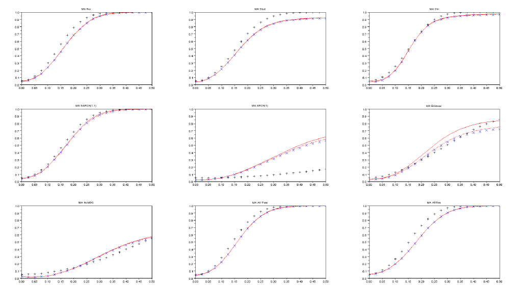
Figure 1. Empirical rejection probabilities of $LOT$ (black ‘+’ line), $Parz$ (red solid line), $BP$ (red dotted line) and Lee (2007) $\widetilde{\mathcal{M}}^{EP32}$ test (blue ‘x’ line). The level of these tests is $5\%$ . The alternative is an $MA(1)$ with a moving average coefficient ranging from $0$ to $1/2$ and disturbances as in Tables 2-3. The sample size is $n=200$ and the number of replications is $10,000$.

The second experiment under $\mathcal{H}_{1}$ examines, for $n=200$, the power of the $5\%$ level $BP$ and $Parz$ tests against $H_{\rho}:u_{t}=v_{t}-\rho v_{t-1}$, $\rho\in\left[0,1/2\right]$, under the nine scenarios of Tables 2 and 3. For example, under ‘GARCH(1,1)’ $v_{t}=s_{t}\zeta_{t}$ and $s_{t}^{2}=0.001+0.90s_{t-1}^{2}+0.05v_{t-1}^{2}$ where $\zeta_{t}$ are i.i.d. standard normal innovations while, under ‘ARRes’, the $v_{t}$ are i.i.d. $N\left(0,1\right)$ and $u_{t}=v_{t}-\rho v_{t-1}$ is estimated from the $AR(1)$ model $X_{t}=0.8X_{t-1}+u_{t}$. We do not consider the other tests to avoid undesirable size correction effects, but we compare $BP$ and $Parz$ with $\widetilde{\mathcal{M}}_{n}^{EP32}$ test of Lee (2007) which rejects the null when $n\widehat{R}_{1}^{2}\geq\widehat{z}\left(\alpha\right)$ where $\widehat{z}\left(\alpha\right)$ is defined in (2.7), and an $\alpha$ level test which rejects the null when $n\widehat{R}_{1}^{2}\geq c\left(\alpha\right)$, where the infeasible $c\left(\alpha\right)$, dependent of the white noise process under consideration, is computed from $10,000$ preliminary replications. Since the latter is locally optimal under Gaussianity, it is labelled $LOT$. Figure 1 reports the nine power graphs corresponding to each white noise experiments.

[INSERT FIGURE 1 HERE]

Except for white noise processes such as ‘NoMDS’ for which the new tests are undersized, the power of the four tests are quite similar in the vicinity of $\rho=0$, suggesting that our data-driven tests are, for processes close to Gaussianity, not far from being locally optimal as $LOT$. The global performance of all tests deteriorate for nonlinear white noise processes as ‘ARCH(1)’, for which $LOT$ has a very low power compared to its competitors $BP$, $Parz$ and $\widetilde{\mathcal{M}}_{n}^{EP32}$. $Parz$ dominates its competitors for such white noise processes. As expected from (3.8), $Parz$ and $BP$ perform as well as or better than $\widetilde{\mathcal{M}}_{n}^{EP32}$ which is less powerful than $Parz$ for heteroskedastic noises the ‘Bilinear’, ‘ARCH(1)’, ‘GARCH(1,1)’ or ‘NoMDS’.

The third experiment under $\mathcal{H}_{1}$ considers a second set of alternatives given by randomized “small correlation” processes defined in (4.1),

$$u_{t}=\varepsilon_{t}+\frac{\left(2.5\times\gamma_{n}\right)^{1/2}}{n^{1/2}P^{1/4}}\sum_{k=1}^{P}\psi_{k,b}\varepsilon_{t-k}\text{,\quad\quad\quad\quad}\psi_{k,b}\overset{\text{i.i.d.}}{\sim}N\left(0,1\right)\text{.}$$ (5.1)

In this setting $b$ is the simulation index, $b=1,...,10,000$. New moving average coefficients $\left\{\psi_{k,b}\right\}$ are drawn for each simulation. Randomizing the moving average coefficients allows us to explore various shapes of the correlation function. The noise $\left\{\varepsilon_{t}\right\}$ is independent of the moving average coefficients $\left\{\psi_{k,b}\right\}$ and is drawn randomly from the standard normal distribution. Since $\sum_{k=1}^{P}\psi_{k,b}^{2}=P\left(1+o_{\mathbb{P}}\left(1\right)\right)$ when $P$ tends to infinity, the covariances of (5.1) can be $o\left(n^{-1/2}\right)$ as shown in Lemma 1. We consider two scenarios. In the experiment ‘LOW’, $P$ is set to $15$ for $n=200$ and to $75$ when $n=1,000$. The experiment ‘HIGH’ doubles the order $P$, so $P=30$ for $n=200$ and $P=150$ for $n=1,000$. The next table reports simulation results.

[INSERT TABLE 5 HERE]

The $BP$ test outperforms its competitors and $Parz$ comes as a second-best. The $EL$ test achieves power similar to that of the $BP$ test only in the LOW experiment when $P=15$ and $n=200$. The power of the $IMSE$ and $CvM$ tests decreases with the sample size while the power of the other tests increases, showing the importance of a proper data-driven choice of the order. The high values of $\overline{\widehat{p}^{\ast}}_{Parz}$ may suggest that the $Parz$ test would be negatively affected by choosing a lower value of $\overline{p}_{n}$. However setting $\overline{p}_{n}=3\left[\left(n/2\right)^{1/2}\right]$ instead of $\overline{p}_{n}=n-1$ as done in an experiment not reported does not really affect the power of the $BP$ test.

6. Concluding remarks

The paper proposes an automatic test for the weak white noise null hypothesis for observed variables or residuals from a parametric model. The test is based on a new data-driven order selection procedure applied to the Box-Pierce (1970) test statistic. The critical region uses robust critical values of Lee (2007) which can account for estimation of residuals. An important theoretical finding is that the new test can detect alternatives with small autocorrelation coefficients of order $\rho_{n}=o\left(n^{-1/2}\right)$ where $n$ is the sample size, provided that the number of autocorrelation coefficients at moderate lags is large enough. The proposed test is shown to be adaptive rate-optimal against this class of alternatives. The paper gives examples of moving average alternatives with small autocorrelation coefficients of order $o\left(n^{-1/2}\right)$ which are detected by the new test but not by tests previously proposed by Deo (2000), Escanciano and Lobato (2009) or Xiao and Wu (2011). These alternatives correspond to a plausible macroeconomic scenario where a temporary shock has no significant impact whereas permanent shocks may cause significant changes. They can also be of interest in finance where arbitrage should rule out strong deviations from the difference of martingale hypothesis, since these alternatives generate conditional expectation given the past of these alternatives with order $o_{\mathbb{P}}\left(n^{-1/2}\right)$. A simulation experiment has shown that the new test can cope with various weak types of white noise processes including the ARCH or GARCH processes popular in empirical finance. The simulation experiment has also confirmed good power properties of the test regarding detection of standard $AR(1)$ and $MA(1)$ alternatives when the noise is highly nonlinear, for instance in the case of the $ARCH(1)$ process considered in the experiment.

7. References

Anderson, T.W. (1993). Goodness of Fit Tests for Spectral Distributions. The Annals of Statistics 21, 830–847.

Anderson, T.W. and D.A. Darling (1952). Asymptotic Theory of Certain “Goodness of Fit” Criteria Based on Stochastic Processes. Annals of Mathematical Statistics 23, 193–212.

Box, G. and D. Pierce (1970). Distribution of Residual Autocorrelations in Autoregressive-Integrated Moving Average Time Series Models. Journal of American Statistical Association 65, 1509–1526.

Campbell, J.Y., A.W. Lo and A.C. Craig MacKinlay (1997). The Econometrics of Financial Markets. Second Edition, Princeton University Press.

Chen, S.X. and J. Gao (2007). An adaptive Empirical Likelihood Test for Parametric Time Series Regression Models. Journal of Econometrics 141, 950–972.

Delgado, M.A. and C. Velasco (2012). An Asymptotically Pivotal Transform of the Residuals Sample Autocorrelations with Application to Model Checking. Journal of American Statistical Association 106, 646—958.

Delgado, M.A., J. Hidalgo and C. Velasco (2005). Distribution Free Goodness-of-Fit Tests for Linear Processes. The Annals of Statistics 33, 2568-2609.

Deo, R.S. (2000). Spectral Tests of the Martingale Hypothesis under Conditional Heteroscedasticity. Journal of Econometrics 99, 291-315.

Donoho, D. and J. Jin (2004). Higher Criticism for Detecting Sparse Heterogeneous Mixtures. The Annals of Statistics 32, 962–994.

Durlauf, S.N. (1991). Spectral Based Testing of the Martingale Hypothesis. Journal of Econometrics 50, 355-376.

Escanciano, J.C. and I.N. Lobato (2009). An Automatic Portmanteau Test for Serial Correlation. Journal of Econometrics 151, 140–149.

Fan, J. (1996). Test of Significance Based on Wavelet Thresholding and Neyman’s Truncation. Journal of the American Statistical Association 91, 674–688.

Fan, J. and Q. Yao (2005). Nonlinear Time Series: Nonparametric and Parametric Methods. Springer.

Francq, C. , R. Roy and J.M. Zakoian (2005). Diagnostic Checking in ARMA Models With Uncorrelated Errors. Journal of the American Statistical Association 100, 532–544.

Golubev, G.K., M. Nussbaum and H.H. Zhou (2010). Asymptotic Equivalence of Spectrum Density Estimation and Gaussian White Noise. The Annals of Statistics 38, 181–214.

Grenander, U. and M. Rosenblatt (1952). On Spectral Analysis of Stationary Time-series. Proceedings of the National Academy of Sciences U.S.A. 38, 519-521.

Guay, A. and E. Guerre (2006). A Data-Driven Nonparametric Specification Test for Dynamic Regression Models. Econometric Theory 22, 543–586.

Guerre, E. and P. Lavergne (2002). Optimal Minimax Rates for Nonparametric Specification Testing in Regression Models. Econometric Theory 18, 1139–1171.

Guerre, E. and P. Lavergne (2005). Rate-Optimal Data-Driven Specification Testing for Regression Models. The Annals of Statistics 33, 840–870.

Hong, Y. (1996). Consistent Testing for Serial Correlation of Unknown Form. Econometrica 64, 837–864.

Hong, Y. and Y.J. Lee. (2005). Generalized Spectral Tests for Conditional Mean Models in Time Series with Conditional Heteroscedasticity of Unknown Form. Review of Economic Studies 72, 499–541.

Horowitz, J.L. and V.G. Spokoiny (2001). An Adaptive, Rate-Optimal Test of a Parametric Mean-Regression Model Against a Nonparametric Alternative. Econometrica 69, 599–631.

Kuan, C.M. and W.M. Lee (2006). Robust M Tests without Consistent Estimation of the Asymptotic Covariance Matrix. Journal of the American Statistical Association 101, 1264–1275.

Lee, W.M. (2007). Robust M Tests Using Kernel-based Estimators with Bandwidth Equal to Sample Size. Economics Letters 96, 295–300.

Lobato, I.N. (2001). Testing That a Dependent Process Is Uncorrelated. Journal of the American Statistical Association 96, 1066–1076.

Lobato, I.N., J.C. Nankervis and N.E. Savin (2002). Testing for Zero Autocorrelation in the Presence of Statistical Dependence. Econometric Theory 18, 730–743.

Newey, W.K. and K. West (1994). Automatic Lag Selection in Covariance Matrix Estimation. Review of Economic Studies 61, 631–653.

Phillips, P.C.B, Y. Sun & S. Jin (2006). Spectral Density Estimation and Robust Hypothesis Testing Using Steep Origin Kernels Without Truncation. International Economic Review 47, 837–894.

Pollard, D. (2002). A User’s Guide to Measure Theoretic Probability. Cambridge University Press.

Shao, X. (2011a). A Bootstrap-assisted Spectral Test of White Noise under Unknown Dependence. Journal of Econometrics 162, 213–224.

Shao, X. (2011b). Testing for White Noise under Unknown Dependence and its Applications to Goodness-of-Fit for Time Series Models. Econometric Theory 27, 312–343.

Spokoiny, V.G. (1996). Adaptive Hypothesis Testing Using Wavelets. The Annals of Statistics 24, 2477–2498.

Xiao, H. and W.B. Wu (2011). Asymptotic Inference of Autocovariances of Stationary Processes. University of Chicago, arXiv:11053423v1.

Wu, W.B. (2005). Nonlinear System Theory: Another Look at Dependence. Proceedings of the National Academy of Sciences of the United States of America 102, 14150–14154.

Wu, W.B. (2007). Strong Invariance Principles for Dependent Random Variables. The Annals of Probability 35, 2294–2320.

Robust Adaptive Rate-Optimal Testing for the White Noise Hypothesis: Supplementary Material

Alain Guay

Emmanuel Guerre

Štěpána Lazarová

This version: 2nd November 2012

Supplementary Material A: proofs of main results

This section contains the proofs of the results of Section 3. In what follows, a tilde superscript, as in

$$\widetilde{S}_{p}=n\sum_{j=1}^{p}K^{2}\left(\frac{j}{p}\right)\widetilde{R}_{j}^{2}\text{\quad where\quad}\widetilde{R}_{j}=\frac{1}{n}\sum_{t=1}^{n-|j|}u_{t}u_{t+|j|}.$$ (A.1)

indicates that the variables $u_{t}$ are observed. This also leads to define

$$\widetilde{\tau}_{j}=\frac{1}{n}\sum_{t=1}^{n-|j|}u_{t}^{2}u_{t+|j|}^{2},\quad\widetilde{z}_{L}\left(\alpha\right)=\widehat{z}_{L}\left(\alpha\right),\quad\widetilde{z}_{L}^{\ast}\left(\alpha\right)=\widehat{z}_{L}^{\ast}\left(\alpha\right),$$

but we keep the notation $\widehat{p}$. $C$ and $C^{\prime}$ are constants that may vary from line to line but only depend on the constants of the assumptions. Notation $\left[\cdot\right]$ is used for the integer part of a real number and $a\vee b=\max\left(a,b\right)$, $a\wedge b=\min\left(a,b\right)$. Let $\overline{u}_{t}^{t-j}=\overline{u}_{t,n}^{t-j}$ be a copy of $u_{t}=F_{n}\left(\ldots,e_{t-1},e_{t}\right)$ obtained by changing $e_{t-j}$, $e_{t-j-1}$, $\ldots$ into $e_{t-j}^{\prime}$, $e_{t-j-1}^{\prime}$, $\ldots$. Then the condition $\left\|u_{t}-u_{t}^{t-j}\right\|_{a}\leq\delta_{a}\left(j\right)$ ensures that

$$\left\|u_{t}-\overline{u}_{t}^{t-j}\right\|_{a}\leq\Theta_{a}\left(j\right)\text{ where }\Theta_{a}\left(j\right)=\sum_{i=j}^{\infty}\delta_{a}\left(j\right).$$ (A.2)

We first state some intermediary results that are used in the proofs of our main results. These intermediary results are proven in a section called “Supplementary Material B”. Lemma A.2 gives the order of standardization terms $E(p)$, $E_{\Delta}(p)$ and $V_{\Delta}(p)$. Propositions A.1 and A.2 deal with the impact of the estimation of $\theta$. Proposition A.3 is used to study the asymptotic null behavior of the test and to show that $\mathbb{P}\left(\widehat{p}=1\right)\rightarrow 1$ in Theorem 1. Proposition A.3 deals with observed variables or residuals thanks to Propositions A.1 and A.2. Propositions A.4 and A.5 are the key tools for our consistency result, Theorem 2. They dealt with observed variables but are combined with Propositions A.1 and A.2 to deal with estimation errors in the proof of Theorem 2.

Lemma A.2.

Suppose Assumption K holds and that $\overline{p}_{n}/n\leq 1/2$. (i) There exists a constant $C>1$ such that, for $q=1,2$ and for any $1\leq p\leq\overline{p}_{n}$, $\frac{p}{C}\leq\sum_{j=1}^{n-1}\left(1-\frac{j}{n}\right)^{q}K^{2q}\left(\frac{j}{p}\right)\leq Cp$, $\frac{p}{C}\leq\sum_{j=1}^{n-1}K^{2q}\left(\frac{j}{p}\right)\leq Cp$, $V_{\Delta}^{2}(p)\leq Cp$, and $E_{\Delta}(p)\leq\sum_{j=1}^{n-1}\left(K^{2}\left(\frac{j}{p}\right)-K^{2}\left(j\right)\right)\leq Cp^{1/2}V_{\Delta}(p)$; (ii) Under Assumption P, for all $n$ and all $p\in\left[1,\overline{p}_{n}\right]$, $V_{\Delta}(p)\geq C(p-1)^{1/2}$ and $E_{\Delta}(p)\geq 0$.

Lemma A.3.

Suppose Assumptions K, M and R hold. Then the rejection regions $\widetilde{S}_{1}\geq\widetilde{z}_{L}\left(\alpha\right)$, $\widetilde{S}_{1}^{\ast}\geq\widetilde{z}_{L}^{\ast}\left(\alpha\right)$, $\widehat{S}_{1}\geq\widehat{z}_{KL}\left(\alpha\right)$ and $\widehat{S}_{1}^{\ast}\geq\widehat{z}_{KL}^{\ast}\left(\alpha\right)$ are asymptotically of level $\alpha$. Moreover, under $\mathcal{H}_{1}$, $\widehat{z}_{L}\left(\alpha\right)$, $\widetilde{z}_{L}^{\ast}\left(\alpha\right)$, $\widehat{z}_{KL}\left(\alpha\right)$ and $\widehat{z}_{KL}^{\ast}\left(\alpha\right)$ are all $O_{\mathbb{P}}\left(1\right)$.

Lemma A.4.

Under Assumption R, $\sup_{0\leq j\leq n-1}\operatorname*{Var}\left(\widetilde{R}_{j}\right)\leq\frac{C}{n}$.

Proposition A.1.

Suppose Assumptions M, P and R hold. Then $\max_{j\in\left[0,\overline{p}_{n}\right]}\left|\widehat{R}_{j}-\widetilde{R}_{j}\right|=O_{\mathbb{P}}\left(n^{-1/2}\right)$, $\max_{p\in\left[0,n-1\right]}n\sum_{j=1}^{p}\left(\widehat{R}_{j}-\widetilde{R}_{j}\right)^{2}=O_{\mathbb{P}}\left(1\right)$, and

$$\max_{j\in\left[0,n-1\right]}\left|\widetilde{R}_{j}-\left(1-\frac{j}{n}\right)R_{j,n}\right| =O_{\mathbb{P}}\left(\left(\frac{\log n}{n}\right)^{1/2}\right),$$

$$\max_{j\in\left[0,\overline{p}_{n}\right]}\left|\widehat{R}_{j}-R_{j,n}\right| =O_{\mathbb{P}}\left(\left(\frac{\log n}{n}\right)^{1/2}\right),$$

$$\max_{j\in\left[0,n-1\right]}\left(1-\frac{j}{n}\right)\left|\widetilde{\tau}_{j}^{2}-\tau_{j,n}^{2}\right| =O_{\mathbb{P}}\left(\left(\frac{\log n}{n}\right)^{1/2}\right),$$

$$\max_{j\in\left[0,\overline{p}_{n}\right]}\left|\widehat{\tau}_{j}^{2}-\tau_{j,n}^{2}\right| =O_{\mathbb{P}}\left(\left(\frac{\log n}{n}\right)^{1/2}\right).$$

Proposition A.2.

Let Assumptions K, M, P and R hold. Let $\widetilde{S}_{p}$ be as in (A.1). Then

$$\max_{p\in\left[2,\overline{p}_{n}\right]}\frac{|\left(\widehat{S}_{p}-\widehat{S}_{1}\right)-\left(\widetilde{S}_{p}-\widetilde{S}_{1}\right)|}{1+\left(n\sum_{j=1}^{p}R_{j,n}^{2}\right)^{1/2}}=O_{\mathbb{P}}\left(1\right)$$

and for any $p_{n}=O(n^{1/2})$, $\widehat{S}_{p_{n}}-\widetilde{S}_{p_{n}}=O_{\mathbb{P}}\left(1+\left(n\sum_{j=1}^{p_{n}}R_{j,n}^{2}\right)^{1/2}\right).$

Proposition A.3.

Suppose Assumptions K, M, P and R hold and that $\mathcal{H}_{0}$ is true. Then (3.1) ensures that

$$\lim_{n\rightarrow\infty}\mathbb{P}\left(\max_{p\in\left[2,\overline{p}_{n}\right]}\frac{(\widehat{S}_{p}-\widehat{S}_{1})/\widehat{R}_{0}^{2}-E_{\Delta}(p)}{V_{\Delta}(p)}\geq\gamma_{n}\right)=0.$$

Proposition A.4.

Under Assumptions K, P and R, there are some $C,C^{\prime}>0$ such that for $n$ large enough and uniformly in $p\in\left[1,\overline{p}_{n}\right]$,

$$\mathbb{E}\left[\widetilde{S}_{p}\right]-R_{0,n}^{2}E\left(p\right) \geq Cn\sum_{j=1}^{p/2}R_{j,n}^{2}-C^{\prime}R_{0,n}^{2},$$

$$\mathbb{E}\left[\sum_{j=1}^{n-1}K\left(\frac{j}{p}\right)\frac{\widetilde{R}_{j}^{2}}{\tau_{j,n}^{2}}\right]-E\left(p\right) \geq Cn\sum_{j=1}^{p/2}\left(\frac{R_{j,n}}{R_{0,n}}\right)^{2}-C^{\prime}.$$

Proposition A.5.

Under Assumptions K, P and R, there is a constant $C>0$ such that for $n$ large enough and uniformly in $p\in\left[1,\overline{p}_{n}\right]$,

$$\operatorname*{Var}\left(\widetilde{S}_{p}\right) \leq C\left(n\sum_{j=1}^{p}R_{j,n}^{2}+p\right),$$

$$\operatorname*{Var}\left(\sum_{j=1}^{n-1}K\left(\frac{j}{p}\right)\frac{\widetilde{R}_{j}^{2}}{\tau_{j,n}^{2}}\right) \leq C\left(n\sum_{j=1}^{p}\frac{R_{j,n}^{2}}{R_{0,n}^{2}}+p\right).$$

A.1. Proof of Theorem 1

(3.2), (3.1) and Proposition A.3 give that $\lim_{n\rightarrow\infty}\mathbb{P}(\widehat{p}\neq 1)=0$. Hence $\widehat{S}_{\widehat{p}}=\widehat{S}_{1}+o_{\mathbb{P}}\left(1\right)$ and Lemma A.3, which ensures that the retained critical value satisfies $\mathbb{P}\left(\widehat{S}_{1}\geq\widehat{z}\left(\alpha\right)\right)\rightarrow\alpha$, yield that the test (2.7) is asymptotically of level $\alpha$.$\Box$

A.2. Proof of Theorem 2

The definition (2.2) of $\widehat{p}$ gives, for any $p\in\left[1,\overline{p}_{n}\right]$,

$$\widehat{S}_{\widehat{p}} =\arg\max_{p\in\left[1,\overline{p}_{n}\right]}\left\{\widehat{S}_{p}-\widehat{R}_{0}^{2}E\left(p\right)-\gamma_{n}\widehat{R}_{0}^{2}V_{\Delta}\left(p\right)\right\}+\widehat{R}_{0}^{2}E\left(\widehat{p}\right)+\gamma_{n}\widehat{R}_{0}^{2}V_{\Delta}\left(\widehat{p}\right)$$

$$\geq\widehat{S}_{p}-\widehat{R}_{0}^{2}E\left(p\right)-\gamma_{n}\widehat{R}_{0}^{2}V_{\Delta}\left(p\right).$$

Note that this bound implies (3.6). Since the critical value $\widehat{z}\left(\alpha\right)$ in (2.7) is bounded under $\mathcal{H}_{1}$ by Lemma A.3, it is sufficient to find a $p_{n}\in\left[1,\overline{p}_{n}\right]$ such that $\widehat{S}_{p_{n}}-\widehat{R}_{0}^{2}E\left(p_{n}\right)-\gamma_{n}\widehat{R}_{0}^{2}V_{\Delta}\left(p_{n}\right)\overset{\mathbb{P}}{\rightarrow}+\infty$. Let $p_{n}=2P_{n}$ where $P_{n}$ is as in (3.4). Set

$$\mathcal{R}_{n}^{2}=\sum_{j=1}^{P_{n}}\left(\frac{R_{j,n}}{R_{0,n}}\right)^{2}.$$

The detection condition (3.4) gives

$$n\mathcal{R}_{n}^{2}\geq n\rho_{n}^{2}\sum_{j=1}^{P_{n}}\mathbb{I}\left\{\left(\frac{R_{j,n}}{R_{0,n}}\right)^{2}\geq\rho_{n}^{2}\right\}=nN_{n}\rho_{n}^{2}\geq\frac{\kappa_{\ast}^{2}\gamma_{n}p_{n}^{1/2}}{2^{1/2}}\rightarrow\infty,$$ (A.3)

with a constant $\kappa_{\ast}$ which can be chosen as large as needed. Lemmas A.2, A.4, Assumption P which ensures $P_{n}=o\left(n^{1/2}\right)$ and $\gamma_{n}=o\left(n^{1/4}\right)$, and Proposition A.1 for the case of residuals yield that

$$\widehat{S}_{p_{n}}-\widehat{R}_{0}^{2}E\left(p_{n}\right)-\gamma_{n}\widehat{R}_{0}^{2}V_{\Delta}\left(p_{n}\right)$$

$$=\widetilde{S}_{p_{n}}+O_{\mathbb{P}}\left(1+n^{1/2}R_{0,n}\mathcal{R}_{n}\right)-R_{0,n}^{2}E\left(p_{n}\right)-\gamma_{n}R_{0,n}^{2}V_{\Delta}\left(p_{n}\right)+O_{\mathbb{P}}\left(\frac{p_{n}+\gamma_{n}p_{n}^{1/2}}{n^{1/2}}\right)$$

$$\geq\widetilde{S}_{p_{n}}+O_{\mathbb{P}}\left(1+n^{1/2}R_{0,n}\mathcal{R}_{n}\right)-R_{0,n}^{2}E\left(p_{n}\right)-C\gamma_{n}R_{0,n}^{2}p_{n}^{1/2}.$$

Now the Chebyshev inequality, Propositions A.4 and A.5, give

$$\widetilde{S}_{p_{n}}=\mathbb{E}\left[\widetilde{S}_{p_{n}}\right]+O_{\mathbb{P}}\left(\operatorname*{Var}\nolimits^{1/2}\left(\widetilde{S}_{p_{n}}\right)\right)\geq R_{0,n}^{2}E\left(p_{n}\right)+C^{\prime}R_{0,n}^{2}n\mathcal{R}_{n}^{2}+O_{\mathbb{P}}\left(p_{n}^{1/2}+n^{1/2}\mathcal{R}_{n}\right).$$

Hence substituting gives, since $n\mathcal{R}_{n}^{2}\rightarrow\infty$ by (A.3),

$$\widehat{S}_{p_{n}}-\widehat{R}_{0}^{2}E\left(p_{n}\right)-\gamma_{n}\widehat{R}_{0}^{2}V_{\Delta}\left(p_{n}\right)\geq C^{\prime}R_{0,n}^{2}n\mathcal{R}_{n}^{2}\left(1+o_{\mathbb{P}}\left(1\right)\right)-C\gamma_{n}R_{0,n}^{2}p_{n}^{1/2}\left(1+o_{\mathbb{P}}\left(1\right)\right).$$

Since Assumption R ensures that $R_{0,n}^{2}$ stays bounded away from $0$, (A.3) gives that $\widehat{S}_{p_{n}}-\widehat{R}_{0}^{2}E\left(p_{n}\right)-\gamma_{n}\widehat{R}_{0}^{2}V_{\Delta}\left(p_{n}\right)\overset{\mathbb{P}}{\rightarrow}+\infty$ as requested provided $\kappa_{\ast}^{2}>C^{\prime}/C$. $\hfill\square$

A.3. Proof of Theorem 3

Consider first the null hypothesis. As seen from the proof of Theorem 1, it suffices to show that

$$\lim_{n\rightarrow\infty}\mathbb{P}\left(\max_{p\in\left[2,\overline{p}_{n}\right]}\frac{(\widehat{S}_{p}^{\ast}-\widehat{S}_{1}^{\ast})-E_{\Delta}(p)}{V_{\Delta}(p)}\geq\gamma_{n}\right)=0,$$

a statement which implies that $\widehat{p}^{\ast}=1+o_{\mathbb{P}}\left(1\right)$ so that Lemma A.3 implies that the conclusion of Theorem 1 holds for the test based upon $\widehat{S}_{\widehat{p}^{\ast}}^{\ast}$. Since $\left|R_{j,n}\right|\leq\left\|u_{t,n}\right\|_{2}\left\|u_{t,n}-\overline{u}_{t,n}^{t-j}\right\|_{2}$ and

$$\mathbb{E}\left[u_{t-j,n}^{2}u_{t-j,n}^{2}\right] =\mathbb{E}\left[\left(\overline{u}_{t,n}^{t-j}\right)^{2}u_{t-j,n}^{2}\right]+\mathbb{E}\left[\left(u_{t,n}^{2}-\left(\overline{u}_{t,n}^{t-j}\right)^{2}\right)u_{t-j,n}^{2}\right]$$

$$=R_{0,n}^{2}+\mathbb{E}\left[\left(u_{t,n}-\overline{u}_{t,n}^{t-j}\right)\left(u_{t,n}+\overline{u}_{t,n}^{t-j}\right)u_{t-j,n}^{2}\right],$$

(A.2) shows

$$\left|\tau_{j,n}^{2}-R_{0,n}^{2}\right|\leq C\left\|u_{t,n}\right\|_{8}^{3}\Theta_{2}\left(j\right)\leq Cj^{-6}$$ (A.4)

for all $j\geq 1$. Now Lemmas A.2 and A.4, Assumptions K, P and R, and Proposition A.1 give

$$\max_{p\in\left[2,\overline{p}_{n}\right]}\frac{\left|(\widehat{S}_{p}^{\ast}-\widehat{S}_{1}^{\ast})-(\widehat{S}_{p}-\widehat{S}_{1})/\widehat{R}_{0}^{2}\right|}{V_{\Delta}(p)}\leq C\max_{p\in\left[1,\overline{p}_{n}\right]}\frac{\left|\widehat{S}_{p}^{\ast}-\widehat{S}_{p}/\widehat{R}_{0}^{2}\right|}{p^{1/2}}$$

$$\leq C\max_{p\in\left[1,\overline{p}_{n}\right]}\frac{n}{p^{1/2}}\sum_{j=1}^{p}\left(\frac{\widehat{R}_{j}}{\widehat{R}_{0}}\right)^{2}\left\{\left|\frac{\widehat{\tau}_{j}^{2}}{\widehat{R}_{0}^{2}}-\frac{\tau_{j,n}^{2}}{R_{0,n}^{2}}\right|+\left|\frac{\tau_{j,n}^{2}}{R_{0,n}^{2}}-1\right|\right\}$$

$$\leq Cn\overline{p}_{n}^{1/2}O_{\mathbb{P}}\left(\left(\frac{\log n}{n}\right)^{3/2}\right)+O_{\mathbb{P}}\left(1\right)n\sum_{j=1}^{\overline{p}_{n}}\frac{\widehat{R}_{j}^{2}}{j^{6}}$$

$$=o_{\mathbb{P}}\left(1\right)+O_{\mathbb{P}}\left(\sum_{j=1}^{\overline{p}_{n}}\frac{\operatorname*{Var}\left(n^{1/2}\widehat{R}_{j}\right)}{j^{6}}\right)=O_{\mathbb{P}}\left(1\right).$$

Hence (3.1) and Proposition A.3

$$\mathbb{P}\left(\max_{p\in\left[2,\overline{p}_{n}\right]}\frac{(\widehat{S}_{p}^{\ast}-\widehat{S}_{1}^{\ast})-E_{\Delta}(p)}{V_{\Delta}(p)}\geq\gamma_{n}\right)$$

$$\text{ }=\mathbb{P}\left(\max_{p\in\left[2,\overline{p}_{n}\right]}\frac{(\widehat{S}_{p}-\widehat{S}_{1})/\widehat{R}_{0}^{2}-E_{\Delta}(p)}{V_{\Delta}(p)}+O_{\mathbb{P}}\left(1\right)\geq\gamma_{n}\right)$$

$$\text{ }\leq\mathbb{P}\left(\max_{p\in\left[2,\overline{p}_{n}\right]}\frac{(\widehat{S}_{p}-\widehat{S}_{1})/\widehat{R}_{0}^{2}-E_{\Delta}(p)}{V_{\Delta}(p)}\geq\left(1+\frac{\epsilon}{2}\right)\left(2\ln\ln n\right)^{1/2}\right)+o\left(1\right)$$

$$\text{ }\mathbb{=}o\left(1\right),$$

which gives the desired result under $\mathcal{H}_{0}$.

Consider now Theorem 2 and $\mathcal{H}_{1}$. Define

$$\widehat{S}_{p}^{\bigstar}=n\sum_{j=1}^{p}K^{2}\left(\frac{j}{p}\right)\frac{\widehat{R}_{j}^{2}}{\tau_{j,n}^{2}},\quad\widetilde{S}_{p}^{\bigstar}=n\sum_{j=1}^{p}K^{2}\left(\frac{j}{p}\right)\frac{\widetilde{R}_{j}^{2}}{\tau_{j,n}^{2}}.$$

Let $P_{n}$ be as in (3.4) and define $p_{n}=2P_{n}$ and $\mathcal{R}_{n}$ as in the proof of Theorem 2. Then Assumptions K and R, Propositions A.1 and A.2

$$\left|\widehat{S}_{p_{n}}^{\ast}-\widehat{S}_{p_{n}}^{\bigstar}\right| \leq Cn\sum_{j=1}^{p_{n}}\frac{\widehat{R}_{j}^{2}}{\tau_{j,n}^{2}}\left|\frac{\tau_{j,n}^{2}}{\widehat{\tau}_{j}^{2}}-1\right|=O_{\mathbb{P}}\left(\left(\frac{\log n}{n}\right)^{1/2}\right)\check{S}_{p_{n}}^{\bigstar},$$

$$\left|\widehat{S}_{p_{n}}^{\bigstar}-\widetilde{S}_{p_{n}}^{\bigstar}\right| \leq C\left|\widehat{S}_{p_{n}}-\widetilde{S}_{p_{n}}\right|=O_{\mathbb{P}}\left(n^{1/2}\mathcal{R}_{n}\right).$$

Hence, for observed variables or residuals,

$$\widehat{S}_{p_{n}}^{\ast}=\left(1+O_{\mathbb{P}}\left(\left(\frac{\log n}{n}\right)^{1/2}\right)\right)\widetilde{S}_{p_{n}}^{\bigstar}+O_{\mathbb{P}}\left(n^{1/2}\mathcal{R}_{n}\right)$$

The proof now follows the steps of the one of Theorem 2 based on the order above, Proposition A.4 and A.5, and Lemma A.4 which gives $\mathbb{E}\left[\widetilde{S}_{p_{n}}^{\bigstar}\right]\leq C\left(p_{n}+n\mathcal{R}_{n}^{2}\right)$. Hence, since $p_{n}=o\left(\left(\log n/n\right)^{1/2}\right)$,

$$\widehat{S}_{\widehat{p}^{\ast}}^{\ast} =\arg\max_{p\in\left[1,\overline{p}_{n}\right]}\left\{\widehat{S}_{p}^{\ast}-E\left(p\right)-\gamma_{n}V_{\Delta}\left(p\right)\right\}+E\left(\widehat{p}^{\ast}\right)+\gamma_{n}V_{\Delta}\left(\widehat{p}^{\ast}\right)$$

$$\geq\widehat{S}_{p_{n}}^{\ast}-E\left(p_{n}\right)-C\gamma_{n}p_{n}^{1/2}$$

$$=\left(1+O_{\mathbb{P}}\left(\left(\frac{\log n}{n}\right)^{1/2}\right)\right)\left(\mathbb{E}\left[\widetilde{S}_{p_{n}}^{\bigstar}\right]+\operatorname*{Var}\nolimits^{1/2}\left(\widetilde{S}_{p_{n}}^{\bigstar}\right)\right)-E\left(p_{n}\right)-C\gamma_{n}p_{n}^{1/2}$$

$$=C^{\prime}R_{0,n}^{2}n\mathcal{R}_{n}^{2}-C\gamma_{n}R_{0,n}^{2}p_{n}^{1/2}+O_{\mathbb{P}}\left(p_{n}^{1/2}+n^{1/2}\mathcal{R}_{n}+\left(\frac{\log n}{n}\right)^{1/2}\left(p_{n}+n\mathcal{R}_{n}^{2}\right)\right)$$

$$=C^{\prime}R_{0,n}^{2}n\mathcal{R}_{n}^{2}\left(1+o_{\mathbb{P}}\left(1\right)\right)-C\gamma_{n}R_{0,n}^{2}p_{n}^{1/2}\left(1+o_{\mathbb{P}}\left(1\right)\right)\overset{\mathbb{P}}{\rightarrow}+\infty$$

provided $\kappa_{\ast}$ is large enough.$\hfill\square$

A.4. Proof of Theorem 4

Since $\mathbb{P}\left(\widehat{p}^{\ast}=1\right)\rightarrow 1$ under $\mathcal{H}_{0}$, condition (A0) and (3.7) give

$$\lim_{n\rightarrow\infty}\mathbb{P}\left(\widehat{S}_{\widehat{p}^{\ast}}^{\ast}\geq\widehat{c}_{n}^{\ast}\left(\alpha\right)\right) =\lim_{n\rightarrow\infty}\mathbb{P}\left(\widehat{S}_{1}^{\ast}\geq\widehat{c}_{n}^{\ast}\left(\alpha\right)\right)=\lim_{n\rightarrow\infty}\mathbb{P}\left(\widehat{S}_{1}^{\ast}\geq\widehat{S}_{1}^{\ast}-\widehat{T}_{n}+\widehat{t}_{n}\left(\alpha\right)\right)$$

$$=\lim_{n\rightarrow\infty}\mathbb{P}\left(\widehat{T}_{n}\geq\widehat{t}_{n}\left(\alpha\right)\right)=\alpha,$$

so that the test of interest is asymptotically of level $\alpha$. Let us now consider the alternative. Arguing as in the proof of Theorems 2 and 3 under condition (A1) shows that the test with critical value $\widehat{c}_{n}\left(\alpha\right)$ detects the alternatives (3.4) provided $\kappa_{\ast}$ is taken large enough. Consider now (3.8). The definition of (2.9) gives, since $E_{\Delta}\left(\widehat{p}^{\ast}\right)+\gamma_{n}V_{\Delta}(\widehat{p}^{\ast})\geq 0$ under Assumption K,

$$\widehat{S}_{\widehat{p}^{\ast}}^{\ast} =\max_{p\in\left[1,\overline{p}_{n}\right]}\left(\widehat{S}_{p}^{\ast}-E_{\Delta}\left(p\right)-\gamma_{n}V_{\Delta}(p)\right)+E_{\Delta}\left(\widehat{p}^{\ast}\right)+\gamma_{n}V_{\Delta}(\widehat{p}^{\ast})$$

$$\geq\widehat{S}_{1}^{\ast}-E_{\Delta}\left(1\right)-\gamma_{n}V_{\Delta}(1)=\widehat{S}_{1}^{\ast}.$$

Hence, by (3.7)

$$\mathbb{P}\left(\widehat{S}_{\widehat{p}^{\ast}}^{\ast}\geq\widehat{c}_{n}\left(\alpha\right)\right)\geq\mathbb{P}\left(\widehat{S}_{1}^{\ast}\geq\widehat{c}_{n}\left(\alpha\right)\right)=\mathbb{P}\left(\widehat{S}_{1}^{\ast}\geq\widehat{S}_{1}^{\ast}-\widehat{T}_{n}+\widehat{t}_{n}\left(\alpha\right)\right)=\mathbb{P}\left(\widehat{T}_{n}\geq\widehat{t}_{n}\left(\alpha\right)\right),$$

which is (3.8).$\hfill\square$

A.5. Proof of Theorem 5

We first introduce a set of alternatives. Let $f\left(\cdot\right)$ denote the spectral density of a centered Gaussian stationary process $\left\{u_{t}\right\}.$with covariance coefficients $R_{j}$. Define a Hölder class of  processes as

$$\text{H\"{o}lder}\left(L\right)=\left\{\left\{u_{t}\right\}\text{: }1/3\leq\inf_{\lambda\in\left[-\pi,\pi\right]}f\left(\lambda\right)\leq\sup_{\lambda\in\left[-\pi,\pi\right]}f\left(\lambda\right)\leq 3\text{, }\sup_{\lambda\in\left[-\pi,\pi\right]}\left|f^{\prime}\left(\lambda\right)\right|\leq L,\text{ }\sum_{j=0}^{\infty}\left|R_{j}\right|\leq L\right\}.$$

The next Lemma describes a family of alternatives which satisfies Assumption R uniformly for prescribed constants and a given $\delta_{a}\left(j\right).$

Lemma A.5.

Consider a centered stationary Gaussian process $\left\{u_{t}\right\}$ with spectral density function $f\left(\lambda\right)=\exp\left(g\left(\lambda\right)\right)/\left(2\pi\right)$, where

$$g\left(\lambda\right)=2\rho\sum_{k=1}^{p}b_{k}\cos\left(k\lambda\right),\text{\quad\quad\quad\quad}b_{k}=-1,0,1.$$ (A.5)

If $p\geq 1$ and $\rho\geq 0$ are such that $p^{2}\rho\leq\epsilon\leq 1/6$ then there is some constant $L>0$, independent of $\epsilon$, $p$, $\rho$ and $b=\left(b_{k},k\in\left[1,p\right]\right)$, such that (i) $\left|R_{0}-1\right|\leq 6\rho\epsilon$ and $\left|R_{j}-\rho b_{j}\right|\leq 6\rho\epsilon$ for $j\in\left[1,p\right]$; (ii) $\left|R_{j}\right|\leq 3\rho\left(2\epsilon\right)^{\ell}$ for all $j$ in $\left[\ell p+1,\left(\ell+1\right)p\right)$ and all $\ell\geq 1$; (iii) $\left\{u_{t}\right\}$ is in Hölder$\left(L\right)$; (iv) Suppose that $\rho_{n}^{2}=\rho_{n}^{2}(p)=2\kappa_{n}^{2}\left(2\log\log n\right)^{1/2}/\left(np^{1/2}\right)$ for some $\kappa_{n}>0$ and bounded away from infinity, and that $p\in\left[1,P_{n}\right]$ with $P_{n}=o\left(\left(n/\left(\kappa_{n}^{2}\log\log n\right)^{1/2}\right)^{1/14}\right)$. Then the associated family of processes $\left\{u_{t}\left(b,p\right);b\in\left\{-1,0,1\right\}^{p},p\in\left[1,P_{n}\right]\right\}$ satisfies Assumption R for any $a>0$ and a $\delta_{a}\left(j\right)=O\left(j^{-7-1/4}\right)$.

Proof of Lemma A.5. Rewrite $g$ as $g\left(\lambda\right)=\rho\sum_{k=-p}^{p}b_{k}\exp\left(ik\lambda\right)$, $b_{0}=0$, $b_{k}=b_{-k}=b_{\left|k\right|}$. Since $\exp\left(x\right)=\sum_{m=0}^{\infty}x^{m}/m!$ uniformly over any compact set and $\max_{\lambda}\left|g\left(\lambda\right)\right|\leq 2p\rho\leq 2\epsilon\leq 1/3$, we have

$$R_{j}=\int_{-\pi}^{\pi}\exp\left(-ij\lambda\right)f\left(\lambda\right)d\lambda=\frac{1}{2\pi}\sum_{m=0}^{\infty}\frac{1}{m!}\int_{-\pi}^{\pi}\exp\left(-ij\lambda\right)\left(g\left(\lambda\right)\right)^{m}d\lambda.$$ (A.6)

For $m>0$, since $\int_{-\pi}^{\pi}\exp\left(-ij\lambda\right)d\lambda=2\pi$ if $j=0$ and $0$ if $j\neq 0$,

$$\frac{1}{2\pi}\int_{-\pi}^{\pi}\exp\left(-ij\lambda\right)\left(g\left(\lambda\right)\right)^{m}d\lambda$$

$$=\frac{\rho^{m}}{2\pi}\sum_{\left(k_{1},...,k_{m}\right)\in K_{m}}b_{k_{1}}\times\cdots\times b_{k_{m}}\int_{-\pi}^{\pi}\exp\left(i\left(k_{1}+\ldots+k_{m}-j\right)\lambda\right)d\lambda$$

$$=\rho^{m}\sum_{\left(k_{1},...,k_{m}\right)\in K_{m}\left(j\right)}b_{k_{1}}\times\cdots\times b_{k_{m}},$$ (A.7)

where $K_{m}$ is the set of $m$-tuples with entries in $\left[-p,p\right]\setminus\left\{0\right\}$ so that $\#K_{m}=\left(2p\right)^{m}$ and $K_{m}\left(j\right)$ contains $m$-tuples in $K_{m}$ for which $k_{1}+\cdots+k_{m}=j$ so that $\#K_{m}(j)\leq\left(2p\right)^{m-1}$.

Proof of (i). Part (i) is a consequence of (A.6), (A.7) and inequality $2p\rho\leq 2\epsilon<1$ which together imply that for $j\in\left[0,p\right]$, $\left|R_{j}-\mathbb{I}\left(j=0\right)-\rho b_{j}\right|\leq\rho\sum_{m=2}^{\infty}\frac{\left(2p\rho\right)^{m-1}}{m!}\leq 2p\rho^{2}\sum_{m=0}^{\infty}\frac{1}{m!}\leq 2e\rho\epsilon<6\rho\epsilon$.

Proof of (ii). Let $\ell p+1\leq j>\left(\ell+1\right)p$. Observe that $K_{m}\left(j\right)$ is an empty set when $m\leq\ell$. Hence it follows from (A.6) and (A.7) that $\left|R_{j}\right|\leq\left|\frac{1}{2\pi}\sum_{m=\ell+1}^{\infty}\frac{1}{m!}\int_{-\pi}^{\pi}\exp\left(-ij\lambda\right)\left(g\left(\lambda\right)\right)^{m}d\lambda\right|\leq\rho\sum_{m=\ell+1}^{\infty}\frac{\left(2p\rho\right)^{m-1}}{m!}\leq\rho\left(2\epsilon\right)^{\ell}e$.

Proof of (iii). Observe that $\left|g\left(\lambda\right)\right|\leq 2\rho p\leq 2\epsilon\leq 1/3$ and that therefore

$$1/3<1-1/3<\exp\left(-1/3\right)\leq f\left(\lambda\right)\leq\exp\left(1/3\right)\leq e\leq 3\quad\quad\quad\quad\text{for all }\lambda\in\left[-\pi,\pi\right].$$

Parts (i), (ii) and $0\leq\rho\leq\epsilon<1/6$, $p\rho\leq 1/6$ yield that, for $L$ large enough,

$$\sum_{j=0}^{\infty}\left|R_{j}\right| \leq R_{0}+\sum_{j=1}^{p}\left|R_{j}\right|+\sum_{\ell=1}^{\infty}\sum_{j=\ell p+1}^{\left(\ell+1\right)p}\left|R_{j}\right|\leq 1+6\rho\epsilon+\left(1+6\epsilon\right)p\rho+3\sum_{\ell=1}^{\infty}\left(\ell+1\right)p\rho\left(2\epsilon\right)^{\ell}$$

$$\leq 1+1+1+1+\sum_{\ell=1}^{\infty}\left(\ell+1\right)\left(2\epsilon\right)^{\ell}\leq L.$$

Since $f^{\prime}\left(\lambda\right)=g^{\prime}\left(\lambda\right)f\left(\lambda\right)$ with $g^{\prime}\left(\lambda\right)=-2\rho\sum_{k=1}^{p}b_{k}k\sin\left(k\lambda\right)$, we have $\sup_{\lambda\in\left[-\pi,\pi\right]}\left|f^{\prime}\left(\lambda\right)\right|\leq 3\times 2p^{2}\rho\leq 1$.

Proof of (iv). Let $u_{t}=\varepsilon_{t}+\sum_{j=1}^{\infty}\psi_{j}\varepsilon_{t-j}$ be the Wold decomposition of the process. Brillinger (2001) and $\int_{-\pi}^{\pi}\log f\left(\lambda\right)\exp\left(ij\lambda\right)d\lambda/2\pi=\rho b_{j}$ gives

$$\psi_{j} =\frac{\int_{-\pi}^{\pi}\exp\left(\rho\sum_{k=1}^{p}b_{k}\exp\left(-ik\lambda\right)\right)\exp\left(ij\lambda\right)d\lambda}{\int_{-\pi}^{\pi}\exp\left(\rho\sum_{k=1}^{p}b_{k}\exp\left(-ik\lambda\right)\right)d\lambda},$$

$$\operatorname*{Var}\left(\varepsilon_{t}\right) =\left|\frac{1}{2\pi}\int_{-\pi}^{\pi}\exp\left(\rho\sum_{k=1}^{p}b_{k}\exp\left(-ik\lambda\right)\right)d\lambda\right|^{2}.$$

Arguing as in (i) and (ii) with an expansion as in (A.6) give $\operatorname*{Var}\left(\varepsilon_{t}\right)=1$, $\left|\psi_{j}-\rho b_{j}\right|\leq C\rho\epsilon$ for $j\in\left[1,p\right]$ and $\left|\psi_{j}\right|\leq C\rho\left(2\epsilon\right)^{\ell}$ for all $j\in\left[\ell p+1,\left(\ell+1\right)p\right)$ and all $\ell\geq 1$. Gaussianity, the choice of $\rho$ in (iv) with the restriction on $P_{n}$ and Wu (2005) give, for any $a>1$, $\delta_{12a}\left(j\right)\leq C_{a}\left|\psi_{j}\right|\leq C_{a}j^{-7-1/4}$. That the other conditions of Assumption R hold uniformly in $p\in\left[1,P_{n}\right]$ follows from (i) and (ii).$\hfill\square$

We will now define a family $\mathcal{F}_{n}$ of correlated Gaussian alternatives. We first introduce some notation. Consider $\widetilde{\gamma}_{n}=\left(2\ln\ln n\right)^{1/2}$ and $\mathcal{P}^{\prime}=\left\{2^{j},j=1,\ldots,J_{n}\right\}$, $2^{J_{n}}=P_{n}=o\left(\overline{p}_{n}\wedge\left(n/\widetilde{\gamma}_{n}\right)^{1/14}\right)$ so that $\mathcal{P}^{\prime}\subset\left[1,\overline{p}_{n}\right]$ for $n$ large enough. Define also

$$\rho_{n}^{2}(p)=2\frac{\kappa_{n}^{2}\widetilde{\gamma}_{n}}{np^{1/2}},\quad\widetilde{\rho}_{n}(p)=2\rho_{n}^{2}(p)\quad\epsilon_{n}=P_{n}^{2}\rho_{n}(P_{n})=\frac{\left(\widetilde{\gamma}_{n}\right)^{1/2}\kappa_{n}P_{n}^{7/4}}{n^{1/2}}=o\left(1\right).$$ (A.8)

Since $p^{2}\rho_{n}(p)\leq\epsilon_{n}$ for all $p\in\mathcal{P}^{\prime}$, $\epsilon_{n}$ plays the role of the real number $\epsilon$ of Lemma A.5 and we assume from now on that $n$ is so large that $\epsilon_{n}\leq 1/6$. Consider the following log-spectral density functions:

$$g\left(\lambda;b,p\right)=2\widetilde{\rho}_{n}(p)\sum_{k\in\left[p,2p\right)}b_{k}\cos\left(k\lambda\right),\quad b=\left(b_{1},\ldots,b_{P_{n}}\right)\in\left\{-1,1\right\}^{P_{n}},\quad p\in\mathcal{P}^{\prime}.$$

Functions $g$ are of the form specified in (A.5). Let $W$ be a symmetric standard Brownian motion process. Consider a centered stationary Gaussian processes

$$u_{t,n}\left(b,p\right)=\frac{1}{\left(2\pi\right)^{1/2}}\int_{-\pi}^{\pi}\exp\left(\frac{g\left(\lambda;b,p\right)}{2}\right)\exp\left(it\lambda\right)dW\left(\lambda\right).$$

Observe that $u_{t,n}\left(0,p\right)$ does not depend on $p$ and is a Gaussian white noise process with variance 1. Let $\left\{R_{j,n}\left(b,p\right)\right\}$ denote the covariance function of $u_{t,n}\left(b,p\right)$. The family $\mathcal{F}_{n}$ of Gaussian processes can now be defined as

$$\mathcal{F}_{n}=\left\{\left\{u_{t,n}\left(b,p\right)\right\},b\in\left\{-1,1\right\}^{P_{n}},p\in\mathcal{P}^{\prime}\right\}.$$

Lemma A.5 implies that all sequences $\left\{u_{t,n}\right\}$ in $\mathcal{F}_{n}$ satisfies Assumption R and that $\mathcal{F}_{n}\subset$Hölder$\left(L\right)$. We now study the asymptotic behavior of the stochastic covariance sequence $\left\{R_{j,n}\left(B,P\right)\right\}$. Let $N_{n}\left(b,p\right)$ be as in (3.3), that is

$$N_{n}\left(b,p\right)=N_{n}\left(\left\{u_{t,n}\left(b,p\right)\right\},p,\rho_{n}\left(p\right)\right)=\#\left\{\left|\frac{R_{j,n}\left(b,p\right)}{R_{0,n}\left(b,p\right)}\right|\geq\rho_{n}\left(p\right),\text{ }j\in\left[1,p\right]\right\}.$$

Lemma A.5-(i,ii) and (A.8) gives that $N_{n}\left(b,p\right)=p/2$ for $n$ large enough and uniformly in $p=2^{j}\in\mathcal{P}^{\prime}$, so that $\rho_{n}^{2}(p)=2\kappa_{n}^{2}\widetilde{\gamma}_{n}/\left(np^{1/2}\right)=\kappa_{n}^{2}\widetilde{\gamma}_{n}p^{1/2}/\left(nN_{n}\left(b,p\right)\right)$. Hence the sequences $\left\{u_{t,n}\right\}$ in $\mathcal{F}_{n}$ satisfies condition (i) in Theorem 5. Therefore the Theorem will be proved if we show that $\sup_{T_{n}}\min_{\left\{u_{t,n}\right\}\in\mathcal{F}_{n}}\mathbb{P}\left(T_{n}=0\right)\leq\alpha+o\left(1\right)$, where $\sup_{T_{n}}$ is a supremum over asymptotically $\alpha$-level tests. Since the equivalence result of Golubev et al. (2010) holds over $\mathcal{F}_{n}\subset$Hölder$\left(L\right)$ this is equivalent to show that $\sup_{T_{n}}\min_{\left\{U_{n}\right\}\in\mathcal{F}_{n}}\mathbb{Q}\left(T_{n}=0\right)\leq\alpha+o\left(1\right)$, $\mathbb{Q}$ being the distribution of the continuous time regression model

$$dU_{n}\left(\lambda;b,p\right)=g\left(\lambda;b,p\right)d\lambda+2\pi^{1/2}\frac{dW\left(\lambda\right)}{n^{1/2}},\quad\quad\lambda\in\left[-\pi,\pi\right],$$

where $W\left(\cdot\right)$ is a Brownian motion over $\lambda\in\left[-\pi,\pi\right]$. This can be done as in Spokoiny (1996, Proof of Theorem 2.3) by bounding $\sup_{T_{n}}\min_{\left\{U_{n}\right\}\in\mathcal{F}_{n}}\mathbb{Q}\left(T_{n}=0\right)$ with a Bayes risk, based on the choice of a uniform distribution for $p$ and a Bernoulli one for $b$.$\hfill\square$

A.6. Proof of Lemma 1

The first approximation $R_{0,n}=\sigma^{2}\left(1+O\left(\gamma_{n}P_{n}^{1/2}/n\right)\right)$ follows easily from the definition (4.1) of the alternative. To show that the second approximation is valid, note that for $j=1,...,P_{n}$,

$$R_{j,n}=\frac{\nu\gamma_{n}^{1/2}}{n^{1/2}P_{n}^{1/4}}\psi_{j}\sigma^{2}+\left(\frac{\nu\gamma_{n}^{1/2}}{n^{1/2}P_{n}^{1/4}}\right)^{2}\left(\psi_{j+1}\psi_{1}+\cdot\cdot\cdot+\psi_{P_{n}}\psi_{P_{n}-j}\right)\sigma^{2}.$$

By the Cauchy-Schwarz inequality, $\left|\psi_{j+1}\psi_{1}+\cdot\cdot\cdot+\psi_{P_{n}}\psi_{P_{n}-j}\right|\leq\sum_{k=1}^{P_{n}}\psi_{k}^{2}=O(P_{n})$ for all $j=1,...,P_{n}$, hence, uniformly in $j=1,...,P_{n}$,

$$R_{j,n}=\frac{\nu\gamma_{n}^{1/2}}{n^{1/2}P_{n}^{1/4}}\psi_{j}\sigma^{2}+O\left(\frac{\gamma_{n}P_{n}^{1/2}}{n}\right)=\frac{\nu\gamma_{n}^{1/2}}{n^{1/2}P_{n}^{1/4}}\psi_{j}\sigma^{2}+o\left(\frac{\gamma_{n}^{1/2}}{n^{1/2}P_{n}^{1/4}}\right)$$

since $P_{n}=o((n/\gamma_{n})^{2/3})$.

For the expression of $\mathbb{E}\left[u_{t}|u_{t-k},k\geq 1\right]$, observe that (4.1) gives, for $n$ large enough,

$$\mathbb{E}\left[u_{t}|u_{t-k},k\geq 1\right]=\frac{\nu\gamma_{n}^{1/2}}{n^{1/2}P_{n}^{1/4}}\sum_{k=1}^{P_{n}}\psi_{k}\varepsilon_{t-k}$$

$$\text{ }=\frac{\nu\gamma_{n}^{1/2}}{n^{1/2}P_{n}^{1/4}}\sum_{k=1}^{P_{n}}\psi_{k}\left(u_{t-k}-\frac{\nu\gamma_{n}^{1/2}}{n^{1/2}P_{n}^{1/4}}\sum_{j=1}^{P_{n}}\psi_{j}\varepsilon_{t-k-j}\right)$$

$$\text{ }=\frac{\nu\gamma_{n}^{1/2}}{n^{1/2}P_{n}^{1/4}}\sum_{k=1}^{P_{n}}\psi_{k}u_{t-k}-\frac{\nu^{2}\gamma_{n}}{nP_{n}^{1/2}}\sum_{k=1}^{P_{n}}\psi_{k}\sum_{j=1}^{P_{n}}\psi_{j}\varepsilon_{t-k-j}.$$

Now, since $\left\{\varepsilon_{t}\right\}$ is a strong white noise and $\sum_{k=1}^{P_{n}}\psi_{k}^{2}=O\left(P_{n}\right)$,

$$\frac{\nu^{2}\gamma_{n}}{nP_{n}^{1/2}}\sum_{k=1}^{P_{n}}\psi_{k}\sum_{j=1}^{P_{n}}\psi_{j}\varepsilon_{t-k-j}=\frac{\nu^{2}\gamma_{n}}{nP_{n}^{1/2}}\sum_{\ell=2}^{2P_{n}}\left(\sum_{k=1}^{\max\left(P_{n},\ell-1\right)}\psi_{k}\psi_{\ell-k}\right)\varepsilon_{t-\ell}$$

$$\text{ }=O_{\mathbb{P}}\left(\left(\frac{\gamma_{n}^{2}}{n^{2}P_{n}}\sum_{\ell=2}^{2P_{n}}\left(\sum_{k=1}^{\max\left(P_{n},\ell-1\right)}\psi_{k}\psi_{\ell-k}\right)^{2}\right)^{1/2}\right)$$

$$\text{ }=O_{\mathbb{P}}\left(\left(\frac{\gamma_{n}^{2}\left(\sum_{k=1}^{P_{n}}\psi_{k}^{2}\right)^{2}}{n^{2}}\right)^{1/2}\right)=O_{\mathbb{P}}\left(\frac{\gamma_{n}P_{n}}{n}\right),$$

which ends the proof of the Lemma.$\hfill\Box$

A.7. Proof of Proposition 1

Let us now check consistency of the test (2.7) under the assumption that $\min_{k\in\left[1,P_{n}\right]}\left|\psi_{k}\sigma^{2}\right|\geq 1$. Define $\rho_{n}=\left(\nu/2\right)\gamma_{n}^{1/2}/\left(n^{1/2}P_{n}^{1/4}\right)$. Lemma 1 implies that $N_{n}=P_{n}\left(1+o(1)\right)$ for such a $\rho_{n}$, which therefore satisfies

$$\rho_{n}=\left(1+o\left(1\right)\right)\left(\nu/2\right)\left(\gamma_{n}P_{n}^{1/2}/N_{n}\right)^{1/2}/n^{1/2},$$

so that (3.4) asymptotically holds provided $\nu\geq 3\kappa^{\ast}$ and the test is consistent if $1\leq P_{n}\leq\overline{p}_{n}/2$ by Theorem 2 provided the considered alternatives satisfies Assumption R. Wu (2005) gives that the alternative (4.1) satisfies for any $a>0$,

$$\delta_{12a}\left(j\right)\leq C_{a}\frac{\nu\gamma_{n}^{1/2}}{n^{1/2}P_{n}^{1/4}}\left|\sigma\psi_{j}\right|\text{ for all }j\in\left[1,P_{n}\right]\text{, }\delta_{12a}\left(j\right)=0\text{ for all }j>P_{n}.$$

Hence the condition $P_{n}=O\left(\left(n/\gamma_{n}\right)^{1/14}\right)$ gives that $\delta_{12a}\left(j\right)\leq Cj^{-7-1/4}$ since the $\left|\sigma\psi_{j}\right|$ are bounded away from infinity. Moreover Gaussianity ensures that

$$\left\|u_{t,n}-\varepsilon_{t}\right\|_{12a}\leq C_{a}\sigma\left(\frac{\nu^{2}\gamma_{n}}{nP_{n}^{1/2}}\sum_{k=1}^{P_{n}}\psi_{k}^{2}\right)^{1/2}=O\left(\frac{\nu\gamma_{n}^{1/2}P_{n}^{1/4}}{n^{1/2}}\right)=o\left(1\right),$$

which gives $\operatorname*{Var}\left(u_{t,n}\right)=\sigma^{2}+o\left(1\right)$ and $\max_{j\in\left[1,n\right]}\operatorname*{Var}^{2}\left(u_{t,n}\right)/\operatorname*{Var}\left(u_{t,n}u_{t+j,n}\right)=1+o\left(1\right)$ so that Assumption R holds. This ends the proof of Proposition 1-(i).

Consider now the other tests in Proposition 1-(ii). Define $\widetilde{R}_{1,j}=\sum_{t=1}^{n-j}u_{t,n}u_{t+j,n}/n$, $\widetilde{R}_{0,j}=\sum_{t=1}^{n-j}\varepsilon_{t}\varepsilon_{t+j}/n$, $\widetilde{\tau}_{1,j}^{2}=\sum_{t=1}^{n-j}u_{t,n}^{2}u_{t+j,n}^{2}/\left(n-j\right)-n\widetilde{R}_{1,j}^{2}/\left(n-j\right)$ and $\widetilde{\tau}_{0,j}^{2}=\sum_{t=1}^{n-j}\varepsilon_{t}^{2}\varepsilon_{t+j}^{2}/\left(n-j\right)-n\widetilde{R}_{0,j}^{2}/\left(n-j\right)$. Define also $\eta_{t}=\eta_{t,n}=\nu\sum_{k=1}^{\infty}\psi_{k}\varepsilon_{t-k}$, setting $\psi_{k}=0$ for $k>P_{n}$, so that $u_{t,n}=\varepsilon_{t}+\gamma_{n}^{1/2}\eta_{t}/\left(n^{1/2}P_{n}^{1/4}\right)$. We have

$$\left|\widetilde{R}_{j}-\widetilde{R}_{0,j}\right|\leq\frac{\gamma_{n}^{1/2}}{n^{3/2}P_{n}^{1/4}}\left|\sum_{t=1}^{n-j}\eta_{t}\varepsilon_{t+j}\right|+\frac{\gamma_{n}^{1/2}}{n^{3/2}P_{n}^{1/4}}\left|\sum_{t=1}^{n-j}\varepsilon_{t}\eta_{t+j}\right|+\frac{\gamma_{n}}{n^{2}P_{n}^{1/2}}\left|\sum_{t=1}^{n-j}\eta_{t}\eta_{t+j}\right|.$$

The Burkholder inequality gives, for any $a>1$,

$$\left\|\frac{\gamma_{n}^{1/2}}{n^{3/2}P_{n}^{1/4}}\sum_{t=1}^{n-j}\eta_{t}\varepsilon_{t+j}\right\|_{a}\leq C\frac{\gamma_{n}^{1/2}\left(n-j\right)^{1/2}}{n^{3/2}P_{n}^{1/4}}\left\|\eta_{t}\right\|_{a}\leq C\frac{\gamma_{n}^{1/2}P_{n}^{1/4}}{n},$$

$$\left\|\frac{\gamma_{n}^{1/2}}{n^{3/2}P_{n}^{1/4}}\sum_{t=1}^{n-j}\left(\varepsilon_{t}\eta_{t+j}-\psi_{j}\varepsilon_{t}^{2}\right)\right\|_{a}\leq\left\|\frac{\gamma_{n}^{1/2}}{n^{3/2}P_{n}^{1/4}}\sum_{t=1}^{n-j}\varepsilon_{t}\left(\sum_{k=0}^{j-1}\psi_{j}\varepsilon_{t+j-k}\right)\right\|_{a}$$

$$+\left\|\frac{\gamma_{n}^{1/2}}{n^{3/2}P_{n}^{1/4}}\sum_{t=1}^{n-j}\left(\sum_{k=j+1}^{\infty}\psi_{j}\varepsilon_{t+j-k}\right)\varepsilon_{t}\right\|_{a}\leq C\frac{\gamma_{n}^{1/2}P_{n}^{1/4}}{n},$$

$$\left\|\frac{\gamma_{n}^{1/2}}{n^{3/2}P_{n}^{1/4}}\sum_{t=1}^{n-j}\left(\varepsilon_{t}^{2}-\sigma^{2}\right)\right\|_{a}\leq C\frac{\gamma_{n}^{1/2}}{nP_{n}^{1/4}},\quad\left\|\frac{\gamma_{n}}{n^{2}P_{n}^{1/2}}\sum_{t=1}^{n}\eta_{t}^{2}\right\|_{a}\leq\frac{\gamma_{n}}{nP_{n}^{1/2}}\leq C\frac{\gamma_{n}P_{n}^{1/2}}{n},$$

for all $j$. Note also that $\left|\sum_{t=1}^{n-j}\eta_{t}\eta_{t+j}\right|\leq\sum_{t=1}^{n}\eta_{t}^{2}$ and the Markov inequality give for $a$ large enough, since $\gamma_{n}P_{n}^{1/2}=o(n^{1/4})$

$$\max_{j\in\left[1,n\right]}\left|\widetilde{R}_{1,j}-\widetilde{R}_{0,j}\right|^{a}=O_{\mathbb{P}}\left(\max_{j\in\left[1,n\right]}\left|\widetilde{R}_{1,j}-\widetilde{R}_{0,j}\right|^{a}\right)$$

$$\text{ }=O_{\mathbb{P}}\left(\sum_{j=1}^{n}\left\|\frac{\gamma_{n}^{1/2}}{n^{3/2}P_{n}^{1/4}}\sum_{t=1}^{n-j}\eta_{t}\varepsilon_{t+j}+\sum_{t=1}^{n-j}\varepsilon_{t}\eta_{t+j}\right\|_{a}^{a}+\left\|\frac{\gamma_{n}}{n^{2}P_{n}^{1/2}}\sum_{t=1}^{n}\eta_{t}^{2}\right\|_{a}^{a}\right)$$

$$\text{ }=O_{\mathbb{P}}\left(n\left(\frac{\gamma_{n}^{1/2}P_{n}^{1/4}}{n}\right)^{a}+\left(\frac{\gamma_{n}P_{n}^{1/2}}{n}\right)^{a}\right)=o_{\mathbb{P}}\left(\frac{1}{n^{7a/8-1}}+\frac{1}{n^{3a/4}}\right)$$

$$\text{ }=o_{\mathbb{P}}\left(\frac{1}{\left(n\log n\right)^{a/2}}\right).$$

Hence

$$\max_{j\in\left[1,n\right]}\left|\widetilde{R}_{1,j}-\widetilde{R}_{0,j}\right|=o_{\mathbb{P}}\left(\frac{1}{\left(n\log n\right)^{1/2}}\right).$$ (A.9)

Arguing similarly for the $\widetilde{\tau}_{k,j}^{2}$ give, since $J_{n}=O\left(n^{1/2}\right)$

$$\max_{j\in\left[1,J_{n}\right]}\left|\widetilde{\tau}_{1,j}^{2}-\widetilde{\tau}_{0,j}^{2}\right|=o_{\mathbb{P}}\left(\frac{1}{\left(n\log n\right)^{1/2}}\right)\quad,\max_{j\in\left[1,J_{n}\right]}\left|\widetilde{\tau}_{0,j}^{2}-\sigma^{4}\right|=O_{\mathbb{P}}\left(\frac{\log^{1/2}n}{n^{1/2}}\right),$$ (A.10)

where the latter is from Proposition A.1. Note that (A.9) and (A.10) gives (4.8). Let $W_{k,n}$, $CvM_{k,n}$, $EL_{k,n}$ be the statistic computed under $G_{k}$, $k=0,1$, i.e. with $\widetilde{R}_{0,j}/\widetilde{\tau}_{0,j}$ and $\widetilde{R}_{1,j}/\widetilde{\tau}_{1,j}$. Note that (A.9) and (A.10) gives $W_{1,n}=W_{0,n}+o_{\mathbb{P}}\left(1\right)$. (4.8) and Proposition A.1 give

$$\left|CvM_{1,n}-CvM_{0,n}\right|\leq\frac{2}{\pi^{2}}\sum_{j=1}^{J_{n}}\frac{n\left|\left(\widetilde{R}_{1,j}/\widetilde{\tau}_{1,j}+\widetilde{R}_{0,j}/\widetilde{\tau}_{0,j}\right)\left(\widetilde{R}_{1,j}/\widetilde{\tau}_{1,j}-\widetilde{R}_{0,j}/\widetilde{\tau}_{0,j}\right)\right|}{j^{2}}$$

$$\text{ }\leq 2\max_{j\in\left[1,J_{n}\right]}\frac{\left|n^{1/2}\widetilde{R}_{0,j}\right|}{\widetilde{\tau}_{0,j}}\times\max_{j\in\left[1,J_{n}\right]}\left|n^{1/2}\left(\frac{\widetilde{R}_{1,j}}{\widetilde{\tau}_{1,j}}-\frac{\widetilde{R}_{0,j}}{\widetilde{\tau}_{0,j}}\right)\right|\frac{2}{\pi^{2}}\sum_{j=1}^{J_{n}}\frac{1}{j^{2}}$$

$$\text{ }+\max_{j\in\left[1,J_{n}\right]}n\left(\frac{\widetilde{R}_{1,j}}{\widetilde{\tau}_{1,j}}-\frac{\widetilde{R}_{0,j}}{\widetilde{\tau}_{0,j}}\right)^{2}\frac{2}{\pi^{2}}\sum_{j=1}^{J_{n}}\frac{1}{j^{2}}$$

$$\text{ }=n^{1/2}O_{\mathbb{P}}\left(\left(\frac{\log n}{n}\right)^{1/2}\right)n^{1/2}o_{\mathbb{P}}\left(\frac{1}{\left(n\log n\right)^{1/2}}\right)+no_{\mathbb{P}}\left(\frac{1}{n\log n}\right)=o_{\mathbb{P}}\left(1\right),$$

Hence $CvM_{1,n}=CvM_{0,n}+o_{\mathbb{P}}\left(1\right)$. For $EL_{n}$, $W_{1,n}=W_{0,n}+o_{\mathbb{P}}\left(1\right)$ and Xiao and Wu (2011) gives that $\max_{j\in\left[1,J_{n}\right]}\left|\widetilde{R}_{k,j}/\widetilde{\tau}_{k,j}\right|\leq\left(2\ln n\right)^{1/2}\left(1+o_{\mathbb{P}}\left(1\right)\right)$ for $k=0,1$ so that $\mathbb{P}\left(\widehat{\gamma}_{EL}^{\ast}=\ln n\right)\rightarrow 1$ under $G_{0}$ and $G_{1}$.We now show that $\mathbb{P}\left(\widehat{p}_{EL}^{\ast}=1\right)\rightarrow 1$ under $G_{0}$. Propositions A.4 and A.5, (A.10) give

$$\mathbb{P}\left(\widetilde{p}_{0,EL}^{\ast}\neq 1\right)=\mathbb{P}\left(\max_{p\in\left[2,J_{n}\right]}\frac{\widetilde{BP}_{0,p}^{\ast}-\widetilde{BP}_{0,1}^{\ast}}{p-1}>\ln n\right)+o\left(1\right)$$

$$\text{ }=\mathbb{P}\left(\left(1+o_{\mathbb{P}}\left(1\right)\right)\max_{p\in\left[2,J_{n}\right]}\frac{n\sum_{j=2}^{p}\widetilde{R}_{0,j}^{2}/\sigma^{4}}{p-1}>\ln n\right)+o\left(1\right)$$

$$\text{ }=\mathbb{P}\left(\frac{n\sum_{j=2}^{p}\widetilde{R}_{0,j}^{2}/\sigma^{4}}{p-1}>\frac{1}{2}\ln n\text{ for some }p\in\left[2,J_{n}\right]\right)+o\left(1\right)$$

$$\text{ }\leq\sum_{p=2}^{J_{n}}\mathbb{P}\left(\frac{n\sum_{j=2}^{p}\left(\widetilde{R}_{0,j}^{2}/\sigma^{4}-\mathbb{E}\left[\widetilde{R}_{0,j}^{2}/\sigma^{4}\right]\right)}{p-1}>\frac{1}{2}\ln n-\frac{n\sum_{j=2}^{p}\mathbb{E}\left[\widetilde{R}_{0,j}^{2}/\sigma^{4}\right]}{p-1}\right)+o\left(1\right)$$

$$\text{ }\leq\sum_{p=2}^{J_{n}}\frac{\operatorname*{Var}\left(\frac{n\sum_{j=2}^{p}\left(\widetilde{R}_{0,j}^{2}/\sigma^{4}-\mathbb{E}\left[\widetilde{R}_{0,j}^{2}/\sigma^{4}\right]\right)}{p-1}\right)}{\left(\frac{1}{2}\ln n-\frac{1}{p-1}\sum_{j=2}^{p}\left(1-j/n\right)\right)^{2}}+o\left(1\right)$$

$$\text{ }\leq\frac{C}{\log^{2}n}\sum_{p=2}^{J_{n}}\frac{1}{p-1}+o\left(1\right)=O\left(\frac{1}{\log n}\right)+o\left(1\right)=o\left(1\right).$$

Now, observe that Proposition A.1 and (4.8) give

$$\max_{p\in\left[2,J_{n}\right]}\left|\frac{\widetilde{BP}_{0,p}^{\ast}-\widetilde{BP}_{0,1}^{\ast}}{p-1}-\frac{\widetilde{BP}_{1,p}^{\ast}-\widetilde{BP}_{1,1}^{\ast}}{p-1}\right|\leq\max_{p\in\left[2,J_{n}\right]}\left|\frac{n\sum_{j=2}^{p}\left(\widetilde{R}_{0,j}^{2}/\widetilde{\tau}_{0,j}^{2}-\widetilde{R}_{1,j}^{2}/\widetilde{\tau}_{1,j}^{2}\right)}{p-1}\right|$$

$$\text{ }\leq 2\max_{p\in\left[2,J_{n}\right]}\left|n^{1/2}\frac{\widetilde{R}_{0,j}}{\widetilde{\tau}_{0,j}}\right|\times\max_{p\in\left[2,J_{n}\right]}\left|n^{1/2}\left(\frac{\widetilde{R}_{0,j}}{\widetilde{\tau}_{0,j}}-\frac{\widetilde{R}_{1,j}}{\widetilde{\tau}_{1,j}}\right)\right|+\left(\max_{p\in\left[2,J_{n}\right]}\left|n^{1/2}\left(\frac{\widetilde{R}_{0,j}}{\widetilde{\tau}_{0,j}}-\frac{\widetilde{R}_{1,j}}{\widetilde{\tau}_{1,j}}\right)\right|\right)^{2}$$

$$\text{ }=n^{1/2}O_{\mathbb{P}}\left(\left(\frac{\log n}{n}\right)^{1/2}\right)n^{1/2}o_{\mathbb{P}}\left(\frac{1}{\left(n\log n\right)^{1/2}}\right)+no_{\mathbb{P}}\left(\frac{1}{n\log n}\right)=o_{\mathbb{P}}\left(1\right).$$

This, since arguing as in the bound above gives $\max_{p\in\left[2,J_{n}\right]}\left|\left(\widetilde{BP}_{0,p}^{\ast}-\widetilde{BP}_{0,1}^{\ast}\right)/\left(p-1\right)\right|=O_{\mathbb{P}}\left(\log^{1/2}n\right)$, implies that $\max_{p\in\left[2,J_{n}\right]}\left|\left(\widetilde{BP}_{1,p}^{\ast}-\widetilde{BP}_{1,1}^{\ast}\right)/\left(p-1\right)\right|\leq\log n$ with a probability tending to $1$ and then $\mathbb{P}\left(\widehat{p}_{EL}^{\ast}=1\right)\rightarrow 1$ under $G_{1}$. Hence (4.8) gives that $EL_{1,n}=\widetilde{BP}_{1,1}^{\ast}+o_{\mathbb{P}}\left(1\right)=\widetilde{BP}_{0,1}^{\ast}+o_{\mathbb{P}}\left(1\right)=EL_{0,n}+o_{\mathbb{P}}\left(1\right)$, so that $EL_{n}$ converges in distribution to a Chi square one with one degree of freedom under $G_{0}$ and $G_{1}$.$\Box$

Supplementary Material B: Proofs of intermediary results

The proofs also use the notion of cumulants, see for example Brillinger (2001, p. 19) or Xiao and Wu (2011) for a definition. Let

$$\mathrm{Cum}\left(u_{t_{1,n}},\ldots,u_{t_{q,n}}\right)=\Gamma_{n}(t_{1},\ldots,t_{q})$$

stands for the $q$th cumulants of $\left\{u_{t,n}\right\}$. The next theorem on cumulant summability is Theorem 21 in Xiao and Wu (2011). These authors do not formally consider sequences $\left\{u_{t,n}\right\}$ but the following result is a straightforward extension of Xiao and Wu (2011).

Theorem B.1 (Xiao and Wu (2011)).

Suppose $\left\{u_{t,n}\right\}$ is stationary for each $n$, with

$$\sup_{n}\left\|u_{t,n}\right\|_{q+1}<\infty\text{ and }\sup_{n}\left\|u_{t,n}-u_{t,n}^{t-j}\right\|_{q}\leq\delta_{q}\left(j\right)\text{ where }\sum_{j=0}^{\infty}j^{q-2}\delta_{q}\left(j\right)<\infty.$$

Then there is a $\mathcal{C}$ which only depends on $\sup_{n}\left\|u_{t,n}\right\|_{q+1}$ and $\sum_{j=0}^{\infty}j^{q-2}\delta_{q}\left(j\right)$ such that

$$\sum_{t_{2},\ldots,t_{q}=-\infty}^{\infty}\left|\Gamma_{n}(0,t_{2},\ldots,t_{q})\right|\leq\mathcal{C}\text{.}$$

In what follows, we drop subscript $n$ in expressions like $u_{t,n}$, $R_{j,n}$, $\Gamma_{n}\left(\cdot\right)$ and $\theta_{n}$ when there is no ambiguity. We denote

$$K_{jp}=K^{2}\left(\frac{j}{p}\right)-K^{2}\left(j\right)\quad\quad\text{and}\quad\quad K_{1n}(p)=\sum_{j=1}^{n-1}K_{jp}.$$ (B.1)

B.1. Proof of Lemma A.2

(i) The first three bounds of the lemma follow directly from Assumption K which implies that $K^{2}\left(j/p\right)\geq K^{2}\left(j\right)$ for all $j$ and $\mathbb{I}(x\in[0,1/2])/C\leq K^{2q}(x)\leq C\mathbb{I}(x\in[0,1])$ for some $C>0$. The Cauchy-Schwarz inequality implies that for any $p\in[1,n/2]$, $E_{\Delta}(p)=\sum_{j=1}^{n-1}\left(1-\frac{j}{n}\right)K_{jp}\leq K_{1n}(p)\leq p^{1/2}\left(\sum_{j=1}^{n-1}k_{j}^{2}(p)\right)^{1/2}\leq Cp^{1/2}V_{\Delta}(p)$, which is the last bound in (i). (ii) Write $p=1+\nu$. Since $p\leq\overline{p}_{n}\leq n/2$, the support of $K\left(\cdot\right)$ is $\left[0,1\right]$ and $K\left(\cdot\right)$ is a decreasing function, we have

$$V_{\Delta}^{2}(p) \geq\frac{1}{2}\times 2\sum_{j=2}^{p}K^{2}\left(\frac{j}{p}\right)\geq\sum_{j=1}^{\nu}K^{2}\left(\frac{1+j}{1+\nu}\right)\geq\sum_{j=1}^{\nu}\int_{j}^{j+1}K^{2}\left(\frac{1+x}{1+\nu}\right)dx$$

$$=\int_{1}^{\nu+1}K^{2}\left(\frac{1+x}{1+\nu}\right)dx=\nu\int_{0}^{1}K^{2}\left(\frac{2+z\nu}{1+\nu}\right)dz.$$

The map $\nu\longmapsto$ $\left(2+z\nu\right)/\left(1+\nu\right)$, $z\in\left[0,1\right)$, is decreasing. Hence, for $\nu\geq 2$, $V_{\Delta}^{2}(p)\geq\nu\int_{0}^{1/2}K^{2}\left(\frac{2+2z}{3}\right)dz\geq C\left(p-1\right)$. Now $V_{\Delta}^{2}(2)\geq 2\left(K^{2}\left(\frac{1}{2}\right)-K^{2}\left(1\right)\right)^{2}>0$ gives the desired result for $V_{\Delta}(p)$. Since $K$ is nonincreasing, $p\longmapsto E_{\Delta}(p)$ is non decreasing and $E_{\Delta}(p)\geq 0$ for all $p\in\mathcal{P}$.$\Box$

B.2. Proof of Lemma A.3

Under $\mathcal{H}_{0}$, The proof repeats the steps of Lee (2007), Lobato (2001) and Kuan and Lee (2006) using the joint FCLT of Assumption M. The joint FCLT of Assumption M gives that the critical values are $O_{\mathbb{P}}\left(1\right)$ under $\mathcal{H}_{1}$.$\Box$

B.3. Proof of Lemma A.4.

Equation (5.3.21) in Priestley (1981) and Theorem B.1 gives uniformly in $j$,

$$\operatorname*{Var}\left(\widetilde{R}_{j}\right) =\frac{1}{n}\sum_{j_{1}=-n+j+1}^{n-j-1}\left(1-\frac{|j_{1}|+j}{n}\right)\left(R_{j_{1}}^{2}+R_{j_{1}+j}R_{j_{1}-j}+\Gamma\left(0,j_{1},j,j_{1}+j\right)\right)$$

$$\leq\frac{2}{n}\sum_{j_{1}=-2n}^{2n}R_{j_{1}}^{2}+\frac{1}{n}\sum_{j_{2},j_{3},j_{4}=-\infty}^{+\infty}\left|\Gamma\left(0,j_{2},j_{3},j_{4}\right)\right|$$

$$\leq\frac{4}{n}\sum_{j=0}^{\infty}R_{j}^{2}+\frac{1}{n}\sum_{j_{2},j_{3},j_{4}=-\infty}^{+\infty}\left|\Gamma\left(0,j_{2},j_{3},j_{4}\right)\right|<C.\hfill\square$$

B.4. Proof of Proposition A.1

For the sake of brevity we assume that $\theta$ is unidimensional. That

$$\max_{j\in\left[0,n-1\right]}\left|\widetilde{R}_{j}-\left(1-\frac{j}{n}\right)R_{j,n}\right| =O_{\mathbb{P}}\left(\left(\frac{\log n}{n}\right)^{1/2}\right),$$

$$\max_{j\in\left[0,n-1\right]}\left(1-\frac{j}{n}\right)\left|\widetilde{\tau}_{j}^{2}-\tau_{j,n}^{2}\right| =O_{\mathbb{P}}\left(\left(\frac{\log n}{n}\right)^{1/2}\right),$$

follow from Xiao and Wu (2011, Theorem 2). Note that these authors do not consider stationary sequences $\left\{u_{t,n}\right\}$ but their arguments carry over under Assumption R. Hence it suffices to study $\max_{j\in\left[0,\overline{p}_{n}\right]}\left|\widehat{R}_{j}-\widetilde{R}_{j}\right|$ and $\max_{j\in\left[0,\overline{p}_{n}\right]}\left|\widehat{\tau}_{j}^{2}-\widetilde{\tau}_{j}^{2}\right|$ since $\overline{p}_{n}/n=o\left(n^{-1/2}\right)$ under Assumption P. We then now show that $\max_{j\in\left[0,\overline{p}_{n}\right]}\left|\widehat{R}_{j}-\widetilde{R}_{j}\right|=O_{\mathbb{P}}\left(n^{-1/2}\right)$. Let $e_{t}=\widehat{u}_{t}-u_{t}$, so that

$$\widehat{R}_{j}=\frac{1}{n}\sum_{t=1}^{n-{j}}\left(u_{t}+e_{t}\right)\left(u_{t+j}+e_{t+j}\right)=\widetilde{R}_{j}+\frac{1}{n}\sum_{t=1}^{n-{j}}\left(u_{t}e_{t+j}+e_{t}u_{t+j}\right)+\frac{1}{n}\sum_{t=1}^{n-{j}}e_{t}e_{t+j}$$

with, by the Cauchy-Schwarz inequality, $\left|\sum_{t=1}^{n-{j}}e_{t}e_{t+j}\right|/n\leq\sum_{t=1}^{n}e_{t}^{2}/n$ and, under Assumption M, for $\widehat{\mathfrak{r}}_{t}=\mathfrak{r}_{t}\left(\widehat{\theta}\right)$,

$$\frac{1}{n}\sum_{t=1}^{n-{j}}u_{t}e_{t+j}=\left(\widehat{\theta}-\theta\right)\frac{1}{n}\sum_{t=1}^{n-{j}}u_{t}u_{t+j}^{\left(1\right)}+\frac{1}{2}\left(\widehat{\theta}-\theta\right)^{2}\frac{1}{n}\sum_{t=1}^{n-{j}}u_{t}u_{t+j}^{\left(2\right)}+\frac{1}{n}\sum_{t=1}^{n-{j}}u_{t}\widehat{\mathfrak{r}}_{t+j}.$$

Now, observe that Assumption M gives $\widehat{\theta}-\theta=O_{\mathbb{P}}\left(n^{-1/2}\right)$, $\max_{t\in\left[1,n\right]}\left|\widehat{\mathfrak{r}}_{t}\right|=o_{\mathbb{P}}\left(1/n\right)$ and

$$\frac{1}{n}\sum_{t=1}^{n}e_{t}^{2}\leq 3\left(\widehat{\theta}-\theta\right)^{2}\frac{1}{n}\sum_{t=1}^{n}\left(u_{t}^{\left(1\right)}\right)^{2}+\frac{3}{4}\left(\widehat{\theta}-\theta\right)^{4}\frac{1}{n}\sum_{t=1}^{n}\left(u_{t}^{\left(1\right)}\right)^{2}+\frac{3}{n}\sum_{t=1}^{n}\left|\widehat{\mathfrak{r}}_{t}\right|=O_{\mathbb{P}}\left(\frac{1}{n}\right),$$

$$\max_{j\in\left[1,n\right]}\left|\frac{1}{n}\sum_{t=1}^{n-{j}}\left(u_{t}\widehat{\mathfrak{r}}_{t+j}+u_{t+j}\widehat{\mathfrak{r}}_{t}\right)\right|\leq\frac{2\max_{t\in\left[1,n\right]}\left|\widehat{\mathfrak{r}}_{t}\right|}{n}\sum_{t=1}^{n-{j}}\left|u_{t}\right|=o_{\mathbb{P}}\left(\frac{1}{n}\right).$$

This gives, uniformly in $j\in\left[1,n\right]$

$$\left|\widehat{R}_{j}-\widetilde{R}_{j}\right|\leq\left|\widehat{\theta}-\theta\right|\left|\mathbb{E}\left[u_{t}u_{t+j}^{\left(1\right)}+u_{t+j}u_{t}^{\left(1\right)}\right]\right|$$

$$\text{ }+\left|\widehat{\theta}-\theta\right|\left|\frac{1}{n}\sum_{t=1}^{n-{j}}\left(u_{t}u_{t+j}^{\left(1\right)}+u_{t+j}u_{t}^{\left(1\right)}-\mathbb{E}\left[u_{t}u_{t+j}^{\left(1\right)}+u_{t+j}u_{t}^{\left(1\right)}\right]\right)\right|+O_{\mathbb{P}}\left(\frac{1}{n}\right).$$ (B.2)

It also follows from Assumption M and $\overline{p}_{n}=o\left(n^{1/2}\right)$ that $\left|\widehat{\theta}-\theta\right|\max_{j\in\left[1,n\right]}\left|\mathbb{E}\left[u_{t}u_{t+j}^{\left(1\right)}+u_{t+j}u_{t}^{\left(1\right)}\right]\right|=O_{\mathbb{P}}\left(1/n^{1/2}\right)$, $n\left(\widehat{\theta}-\theta\right)^{2}\sum_{j=0}^{\infty}\mathbb{E}^{2}\left[u_{t}u_{t+j}^{\left(1\right)}+u_{t+j}u_{t}^{\left(1\right)}\right]=O_{\mathbb{P}}\left(1\right)$, and for $A_{t}\left(j\right)=u_{t}u_{t+j}^{\left(1\right)}+u_{t+j}u_{t}^{\left(1\right)}-\mathbb{E}\left[u_{t}u_{t+j}^{\left(1\right)}+u_{t+j}u_{t}^{\left(1\right)}\right]$

$$\left|\widehat{\theta}-\theta\right|\max_{j\in\left[0,\overline{p}_{n}\right]}\left|\frac{1}{n}\sum_{t=1}^{n-{j}}A_{t}\left(j\right)\right|\leq O_{\mathbb{P}}\left(\frac{1}{n^{1/2}}\right)\sum_{j=0}^{\overline{p}_{n}}\left|\frac{1}{n}\sum_{t=1}^{n-{j}}A_{t}\left(j\right)\right|$$

$$\text{ }=O_{\mathbb{P}}\left(\frac{1}{n}\right)O_{\mathbb{P}}\left(\sum_{j=0}^{\overline{p}_{n}}\mathbb{E}^{1/2}\left[\left(\frac{1}{n^{1/2}}\sum_{t=1}^{n-{j}}A_{t}\left(j\right)\right)^{2}\right]\right)$$

$$\text{ }=O_{\mathbb{P}}\left(\frac{1}{n}\right)O_{\mathbb{P}}\left(\overline{p}_{n}\max_{j\in\left[0,\overline{p}_{n}\right]}\left[\left(\frac{1}{n^{1/2}}\sum_{t=1}^{n-{j}}A_{t}\left(j\right)\right)^{2}\right]\right)=O_{\mathbb{P}}\left(\frac{1}{n^{1/2}}\right),$$

$$n\sum_{j=0}^{n-1}\left(\widehat{\theta}-\theta\right)^{2}\left(\frac{1}{n}\sum_{t=1}^{n-{j}}A_{t}\left(j\right)\right)^{2}$$

$$\text{ }=O_{\mathbb{P}}\left(1\right)\frac{1}{n}O_{\mathbb{P}}\left(\sum_{j=0}^{n-1}\mathbb{E}\left[\left(\frac{1}{n^{1/2}}\sum_{t=1}^{n-{j}}A_{t}\left(j\right)\right)^{2}\right]\right)$$

$$\text{ }=O_{\mathbb{P}}\left(1\right)\frac{1}{n}O_{\mathbb{P}}\left(n\max_{j\in\left[0,n\right]}\mathbb{E}\left[\left(\frac{1}{n^{1/2}}\sum_{t=1}^{n-{j}}A_{t}\left(j\right)\right)^{2}\right]\right)=O_{\mathbb{P}}\left(1\right).$$

This gives $\max_{j\in\left[0,\overline{p}_{n}\right]}\left|\widehat{R}_{j}-\widetilde{R}_{j}\right|=O_{\mathbb{P}}\left(n^{-1/2}\right)$ and $\max_{p\in\left[0,n-1\right]}n\sum_{j=1}^{p}\left(\widehat{R}_{j}-\widetilde{R}_{j}\right)^{2}=$ $O_{\mathbb{P}}\left(1\right)$. The study of $\max_{j\in\left[0,\overline{p}_{n}\right]}\left|\widehat{\tau}_{j}^{2}-\widetilde{\tau}_{j}^{2}\right|$ is similar.$\hfill\square$

B.5. Proof of Proposition A.2

For the sake of brevity we assume that $\theta$ is unidimensional. Since $\widehat{R}_{j}^{2}-\widetilde{R}_{j}^{2}=\left(\widehat{R}_{j}-\widetilde{R}_{j}\right)^{2}+2\widetilde{R}_{j}\left(\widehat{R}_{j}-\widetilde{R}_{j}\right)$, Proposition A.2 is a direct consequence of Proposition A.1 and Lemma B.1 below.

Lemma B.1.

Assume that Assumptions K, M, P and R hold. Then

$$\max_{p\in\left[2,\overline{p}_{n}\right]}\frac{\left|n\sum_{j=1}^{n-1}\left(K^{2}(j/p)-K^{2}(j)\right)\widetilde{R}_{j}\left(\widehat{R}_{j}-\widetilde{R}_{j}\right)\right|}{\left(1+n\sum_{j=1}^{p}R_{j}^{2}\right)^{1/2}}=O_{\mathbb{P}}\left(1\right)$$

and $n\sum_{j=1}^{n-1}K^{2}(j/p_{n})\widetilde{R}_{j}\left(\widehat{R}_{j}-\widetilde{R}_{j}\right)=O_{\mathbb{P}}\left(\left(1+n\sum_{j=1}^{p_{n}}R_{j}^{2}\right)^{1/2}\right)$ for any $p_{n}=O(n^{1/2})$.

Proof of Lemma B.1. We just prove the first equality since the proof of the second is very similar. Define $\overline{R}_{j}=\mathbb{E}\left[\widetilde{R}_{j}\right]=(1-j/n)R_{j}$. We have

$$\left|n\sum_{j=1}^{n-1}K_{jp}\widetilde{R}_{j}\left(\widehat{R}_{j}-\widetilde{R}_{j}\right)\right|\leq C_{n}(p)+D_{n}(p),\text{ where}$$

$$C_{n}(p)=\left|n\sum_{j=1}^{n-1}K_{jp}R_{j}\left(\widehat{R}_{j}-\widetilde{R}_{j}\right)\right|,$$

$$D_{n}(p)=\left|n\sum_{j=1}^{n-1}K_{jp}\left(\widetilde{R}_{j}-\overline{R}_{j}\right)\left(\widehat{R}_{j}-\widetilde{R}_{j}\right)\right|.$$

The Cauchy-Schwarz inequality and Assumption K gives

$$C_{n}(p)\leq C\left(n\sum_{j=1}^{p}R_{j}^{2}\right)^{1/2}\left(n\sum_{j=1}^{p}\left(\widehat{R}_{j}-\widetilde{R}_{j}\right)^{2}\right)^{1/2}.$$

Hence Proposition A.1 yields that $\max_{p\in\left[2,\overline{p}_{n}\right]}|C_{n}(p)/\left(n\sum_{j=1}^{p}R_{j}^{2}\right)^{1/2}|=O_{\mathbb{P}}\left(1\right)$. For $D_{n}(p)$, Assumptions K, M, (B.2) and $\widehat{\mathfrak{r}}_{t}=\mathfrak{r}_{t}\left(\widehat{\theta}\right)$ give

$$\max_{p\in\left[2,\overline{p}_{n}\right]}D_{n}(p) \leq O_{\mathbb{P}}(n^{-1/2})\left(\max_{p\in\left[2,\overline{p}_{n}\right]}D_{1n}(p)+\max_{p\in\left[2,\overline{p}_{n}\right]}D_{2n}(p)\right)+O_{\mathbb{P}}(n^{-1})\max_{p\in\left[2,\overline{p}_{n}\right]}D_{3n}(p)$$

$$+\left(\frac{1}{n}\sum_{t=1}^{n}e_{t}^{2}+2\frac{\max_{t\in\left[1,n\right]}\left|\mathfrak{r}_{t}\right|}{n}\sum_{t=1}^{n}\left|u_{t}\right|\right)\max_{p\in\left[2,\overline{p}_{n}\right]}D_{4n}(p),$$

where $D_{1n}(p)=n\sum_{j=1}^{p}\left|\widetilde{R}_{j}-\overline{R}_{j}\right|\left|\mathbb{E}\left[u_{t}u_{t+j}^{(1)}+u_{t+j}u_{t}^{(1)}\right]\right|$,

$$D_{2n}(p) =n\sum_{j=1}^{p}\left|\widetilde{R}_{j}-\overline{R}_{j}\right|\left|\frac{1}{n}\sum_{t=1}^{n-j}\left(u_{t}u_{t+j}^{(1)}+u_{t+j}u_{t}^{(1)}-\mathbb{E}\left[u_{t}u_{t+j}^{(1)}+u_{t+j}u_{t}^{(1)}\right]\right)\right|,$$

$$D_{3n}(p) =n\sum_{j=1}^{p}\left|\widetilde{R}_{j}-\overline{R}_{j}\right|\left|\frac{1}{n}\sum_{t=1}^{n-j}\left(u_{t}u_{t+j}^{(2)}+u_{t+j}u_{t}^{(2)}\right)\right|,$$

$$D_{4n}(p) =n\sum_{j=1}^{p}\left|\widetilde{R}_{j}-\overline{R}_{j}\right|.$$

By Assumption K and M and by Lemma A.4, we have

$$\mathbb{E}\left[\max_{p\in\left[2,\overline{p}_{n}\right]}D_{1n}(p)\right]\leq Cn\sum_{j=1}^{\overline{p}_{n}}\operatorname*{Var}\nolimits^{1/2}\left(\widetilde{R}_{j}\right)\left|\mathbb{E}\left[u_{t}u_{t+j}^{(1)}+u_{t+j}u_{t}^{(1)}\right]\right|\leq Cn^{1/2},$$

$$\mathbb{E}\left[\max_{p\in\left[2,\overline{p}_{n}\right]}D_{2n}(p)\right] \leq Cn^{1/2}\sum_{j=1}^{\overline{p}_{n}}\operatorname*{Var}\nolimits^{1/2}\left(\widetilde{R}_{j}\right)$$

$$\times\mathbb{E}^{1/2}\left[\left|\frac{1}{n^{1/2}}\sum_{t=1}^{n}\left(u_{t}u_{t+j}^{(1)}+u_{t+j}u_{t}^{(1)}-\mathbb{E}\left[u_{t}u_{t+j}^{(1)}+u_{t+j}u_{t}^{(1)}\right]\right)\right|^{2}\right]$$

$$\leq C\overline{p}_{n},$$

$$\mathbb{E}\left[\max_{p\in\left[2,\overline{p}_{n}\right]}D_{3n}(p)\right]\leq Cn\sum_{j=1}^{\overline{p}_{n}}\operatorname*{Var}\nolimits^{1/2}\left(\widetilde{R}_{j}\right)\mathbb{E}^{1/2}\left[\left|\frac{1}{n}\sum_{t=1}^{n}\left(u_{t}u_{t+j}^{(2)}+u_{t+j}u_{t}^{(2)}\right)\right|^{2}\right]\leq C\overline{p}_{n}n^{1/2},$$

$$\mathbb{E}\left[\max_{p\in\left[2,\overline{p}_{n}\right]}D_{4n}(p)\right]\leq Cn\sum_{j=1}^{\overline{p}_{n}}\mathbb{E}\left[\left|\widetilde{R}_{j}-\overline{R}_{j}\right|\right]\leq Cn\sum_{j=1}^{\overline{p}_{n}}\operatorname*{Var}\nolimits^{1/2}\left(\widetilde{R}_{j}\right)\leq Cn^{1/2}\overline{p}_{n}.$$

The Markov inequality gives us the stochastic orders of magnitude of the four maxima in the bound for $\max_{p\in\left[2,\overline{p}_{n}\right]}D_{n}(p)$. Since $\overline{p}_{n}=O\left(n^{1/2}\right)$ by Assumption P, $\max_{t\in\left[1,n\right]}\left|\widehat{\mathfrak{r}}_{t}\right|=o_{\mathbb{P}}\left(1/n\right)$ and $n^{-1}\sum_{t=1}^{n}e_{t}^{2}=O_{\mathbb{P}}(n^{-1})$ by Assumption M, we have $\max_{p\in\left[2,\overline{p}_{n}\right]}\left|D_{n}(p)\right|=O_{\mathbb{P}}\left(1+\frac{\overline{p}_{n}}{n^{1/2}}\right)=O_{\mathbb{P}}\left(1\right)$. This together with $\max_{p\in\left[2,\overline{p}_{n}\right]}|C_{n}(p)/\left(n\sum_{j=1}^{p}R_{j}^{2}\right)^{1/2}|=O_{\mathbb{P}}\left(1\right)$ shows that the Lemma is proved.$\Box$

B.6. Proof of Proposition A.3

The proof of Proposition A.3 is long and divided in three steps. In the two first steps, we focus on observed variables. In the first step, we approximate the sample covariance $\widetilde{R}_{j}$ by a martingale counterpart $\sum_{t=1}^{n}D_{jt}/n$, $j\in\left[1,\overline{p}_{n}\right]$, as in Shao (2011b), see the notations below and Lemmas B.2, B.3. and B.4. The second step deals with the deviation probability of

$$\frac{n\sum_{j=1}^{p}\left(\frac{1}{n}\sum_{t=j+1}^{n}D_{jt}\right)^{2}\left(K^{2}\left(j/p\right)-K^{2}\left(1\right)\right)-\sigma^{4}E_{\Delta}\left(p\right)}{\sigma^{4}V_{\Delta}\left(p\right)}$$

which is approximated with some Gaussian counterparts through the Lindeberg technique, see Lemma B.5. The third step concludes and explicitly deals with the case of residuals thanks to Propositions A.1 and A.2.

Let us now introduce additional notations. Let $\mathcal{F}_{k}$ be the sigma field generated by $e_{k},e_{k-1},\ldots$. Define $\mathbf{P}_{t}\left[Z\right]=\mathbb{E}\left[Z\left|\mathcal{F}_{t}\right.\right]-\mathbb{E}\left[Z\left|\mathcal{F}_{t-1}\right.\right]$. Wu (2007, Proposition 3) establishes that $\left\|\mathbf{P}_{t}\left[u_{t+k}\right]\right\|_{a}\leq\delta_{a}\left(k\right)$ and Shao (2011b) has shown that

$$\left\|\mathbf{P}_{0}\left[u_{k}u_{k-j}\right]\right\|_{a}\leq 2\left\|u_{k}\right\|_{2a}\left(\delta_{2a}\left(k\right)+\delta_{2a}\left(k-j\right)\mathbb{I}\left(j\leq k\right)\right),$$ (B.3)

which is smaller than $4\left\|u_{k}\right\|_{2a}\delta_{2a}\left(k-j\right)$ when $j\leq k$. Define now the vector of martingale difference $D_{t}=\left[D_{1t},\ldots,D_{\overline{p}_{n}t}\right]^{\prime}$ with

$$D_{jt}=\sum_{k=t}^{\infty}\mathbf{P}_{t}\left[u_{k}u_{k-j}\right]$$

which converges a.s. and satisfies $\mathbb{E}\left[D_{jt}\left|\mathcal{F}_{t-1}\right.\right]=0$, $\max_{j}\mathbb{E}\left[\left|D_{jt}\right|^{a}\right]<\infty$, provided $\left\|u_{t}\right\|_{2a}<\infty$ and $\sum_{k=0}^{\infty}\delta_{2a}\left(k\right)<\infty$. Consider the martingale $M_{j}=M_{jn}=\sum_{t=j+1}^{n}D_{jt}$ which is an approximation of $\widetilde{R}_{j}$. Shao (Lemma A.1, 2011b) gives under Assumption R and for any $\mathfrak{a\in}\left[1,6a\right]$,

$$\left(\mathbb{E}^{\frac{1}{\mathfrak{a}}}\left[\left|\sum_{t=j+1}^{n}u_{t}u_{t-j}-M_{j}\right|^{\mathfrak{a}}\right]\right)^{2}\leq C.$$ (B.4)

We shall also use a $\mathfrak{p}$-dependent version of $D_{t}$, denoted $D_{t}^{{}_{t-\mathfrak{p}+1}}$, with entries

$$D_{jt}^{{}_{t-\mathfrak{p}+1}}=\mathbb{E}\left[D_{jt}\left|e_{t},\ldots,e_{t-\mathfrak{p}+1}\right.\right]=\sum_{k=t}^{\infty}\mathbf{P}_{t}^{\prime}\left[u_{k}u_{k-j}\right],\text{ where}$$ (B.5)

$$\mathbf{P}_{t}^{\prime}\left[Z\right]=\mathbf{P}_{t}^{t-\mathfrak{p}+1}\left[Z\right]=\mathbb{E}\left[Z\left|e_{t},\ldots,e_{t-\mathfrak{p}+1}\right.\right]-\mathbb{E}\left[Z\left|e_{t-1},\ldots,e_{t-\mathfrak{p}+1}\right.\right].$$

Arguing as in Shao (2011b, Lemma A.2-(iii)) gives

$$\left\|D_{jt}-D_{jt}^{{}_{t-\mathfrak{p}+1}}\right\|_{\mathfrak{a}}\leq C\left\|u_{t}\right\|_{2\mathfrak{a}}\Theta_{2\mathfrak{a}}\left(\mathfrak{p-}j\right),\quad\text{for all }j\in\left[1,\mathfrak{p}\right].$$ (B.6)

B.6.1. Martingale approximation and preliminary lemmas

An important property of $D_{t}$ and $D_{t}^{{}_{t-\mathfrak{p}+1}}$ is as follows.

Lemma B.2.

Suppose Assumption K and R hold. Let $K_{jp}$ be as in (B.1). Then for any $p\leq\mathfrak{p}$, $t$, and any $s\leq t-\mathfrak{p}$, $\left\|\sum_{j=1}^{p}K_{jp}D_{js}D_{jt}^{{}_{t-\mathfrak{p}+1}}\right\|_{3a}\leq Cp^{1/2}$.

Proof of Lemma B.2. We have

$$\left\|\sum_{j=1}^{p}K_{jp}D_{js}D_{jt}^{t-\mathfrak{p}+1}\right\|_{3a}$$

$$\quad=\left\|\sum_{j=1}^{p}K_{jp}\sum_{k_{1}=0}^{\infty}\mathbf{P}_{s}\left[u_{s+k_{1}}u_{s+k_{1}-j}\right]\sum_{k_{2}=0}^{\infty}\mathbf{P}_{t}^{\prime}\left[u_{t+k_{2}}u_{t+k_{2}-j}\right]\right\|_{3a}$$

$$\quad\leq\left\|\sum_{j=1}^{p}K_{jp}\sum_{k_{1}=0}^{j-1}\mathbf{P}_{s}\left[u_{s+k_{1}}u_{s+k_{1}-j}\right]\sum_{k_{2}=0}^{j-1}\mathbf{P}_{t}^{\prime}\left[u_{t+k_{2}}u_{t+k_{2}-j}\right]\right\|_{3a}$$ (B.7)

$$\quad+\left\|\sum_{j=1}^{p}K_{jp}\sum_{k_{1}=0}^{j-1}\mathbf{P}_{s}\left[u_{s+k_{1}}u_{s+k_{1}-j}\right]\sum_{k_{2}=j}^{\infty}\mathbf{P}_{t}^{\prime}\left[u_{t+k_{2}}u_{t+k_{2}-j}\right]\right\|_{3a}$$ (B.8)

$$\quad+\left\|\sum_{j=1}^{p}K_{jp}\sum_{k_{1}=j}^{\infty}\mathbf{P}_{s}\left[u_{s+k_{1}}u_{s+k_{1}-j}\right]\sum_{k_{2}=0}^{j-1}\mathbf{P}_{t}^{\prime}\left[u_{t+k_{2}}u_{t+k_{2}-j}\right]\right\|_{3a}$$ (B.9)

$$\quad+\left\|\sum_{j=1}^{p}K_{jp}\sum_{k_{1}=j}^{\infty}\mathbf{P}_{s}\left[u_{s+k_{1}}u_{s+k_{1}-j}\right]\sum_{k_{2}=j}^{\infty}\mathbf{P}_{t}^{\prime}\left[u_{t+k_{2}}u_{t+k_{2}-j}\right]\right\|_{3a}.$$ (B.10)

We have for (B.7)

(B.7) $$=\left\|\sum_{j=1}^{p}K_{jp}\sum_{k_{1}=0}^{p-1}\mathbb{I}\left(k_{1}<j\right)u_{s+k_{1}-j}\mathbf{P}_{s}\left[u_{s+k_{1}}\right]\sum_{k_{2}=0}^{p-1}\mathbb{I}\left(k_{2}<j\right)u_{t+k_{2}-j}\mathbf{P}_{t}^{\prime}\left[u_{t+k_{2}}\right]\right\|_{3a}$$

$$=\left\|\sum_{k_{1}=0}^{p-1}\sum_{k_{2}=0}^{p-1}\left(\sum_{j=k_{1}\vee k_{2}}^{p-1}K_{jp}u_{s+k_{1}-j}u_{t+k_{2}-j}\right)\mathbf{P}_{s}\left[u_{s+k_{1}}\right]\mathbf{P}_{t}^{\prime}\left[u_{t+k_{2}}\right]\right\|_{3a}$$

$$\leq\sum_{k_{1}=0}^{p-1}\sum_{k_{2}=0}^{p-1}\left\|\sum_{j=k_{1}\vee k_{2}}^{p-1}K_{jp}u_{s+k_{1}-j}u_{t+k_{2}-j}\right\|_{6a}\delta_{12a}\left(k_{1}\right)\delta_{12a}\left(k_{2}\right),$$

using $\left\|\mathbf{P}_{t}^{\prime}\left[u_{t+k_{2}}\right]\right\|_{12a}\leq\left\|\mathbf{P}_{t}\left[u_{t+k_{2}}\right]\right\|_{12a}=\delta_{12a}\left(k_{2}\right)$. Now (B.4) and the Burkholder inequality give

$$\left\|\sum_{j=k_{1}\vee k_{2}}^{p-1}K_{jp}u_{s+k_{1}-j}u_{t+k_{2}-j}\right\|_{6a}\leq\left\|\sum_{j=k_{1}\vee k_{2}}^{p-1}K_{jp}D_{t+k_{2}-j,t-s+k_{2}-k_{1}}\right\|_{6a}$$

$$\quad+\left\|\sum_{j=k_{1}\vee k_{2}}^{p-1}K_{jp}\left(u_{s+k_{1}-j}u_{t+k_{2}-j}-D_{t+k_{2}-j,t-s+k_{2}-k_{1}}\right)\right\|_{6a}\leq Cp^{1/2}.$$

Hence (B.7) is smaller than $Cp^{1/2}$. For (B.8), we have since $\left\{u_{s+k_{1}-j},j\in\left[1,k_{1}\right]\right\}$ and $\left\{\mathbf{P}_{t}^{\prime}\left[u_{t+k_{2}}u_{t+k_{2}-j}\right],j\in\left[1,k_{1}\right],k_{2}\geq 0\right\}$ are independent,

(B.8) $$=\left\|\sum_{k_{1}=0}^{p-1}\sum_{k_{2}=0}^{\infty}\left(\sum_{j=k_{1}}^{p-1}K_{jp}u_{s+k_{1}-j}\mathbf{P}_{t}^{\prime}\left[u_{t+k_{2}+j}u_{t+k_{2}}\right]\right)\mathbf{P}_{s}\left[u_{s+k_{1}}\right]\right\|_{3a}$$

$$\leq\sum_{k_{1}=0}^{p-1}\sum_{k_{2}=0}^{\infty}\left\|\sum_{j=k_{1}}^{p-1}K_{jp}u_{s+k_{1}-j}\mathbf{P}_{t}^{\prime}\left[u_{t+k_{2}+j}u_{t+k_{2}}\right]\right\|_{6a}\delta_{6a}\left(k_{1}\right).$$

Let $d_{t}=\sum_{k=t}^{\infty}\mathbf{P}_{t}\left[u_{k}\right]$ be the martingale difference approximation of $u_{t}$, see Wu (2007). Now, since $\left\{u_{s+k_{1}-j},d_{s+k_{1}-j,}j\in\left[1,k_{1}\right]\right\}$ and $\left\{\mathbf{P}_{t}^{\prime}\left[u_{t+k_{2}}u_{t+k_{2}-j}\right],j\in\left[1,k_{1}\right],k_{2}\geq 0\right\}$ are independent, arguing as in the proof of Theorem 1 in Wu (2007), (B.4) and the Burkholder inequality give

$$\left\|\sum_{j=k_{1}}^{p-1}K_{jp}u_{s+k_{1}-j}\mathbf{P}_{t}^{\prime}\left[u_{t+k_{2}+j}u_{t+k_{2}}\right]\right\|_{6a}^{2}$$

$$\text{ }\leq 2\left\|\sum_{j=k_{1}}^{p-1}K_{jp}d_{s+k_{1}-j}\mathbf{P}_{t}^{\prime}\left[u_{t+k_{2}+j}u_{t+k_{2}}\right]\right\|_{6a}^{2}+2\left\|\sum_{j=k_{1}}^{p-1}K_{jp}\left(u_{s+k_{1}-j}-d_{t}\right)\mathbf{P}_{t}^{\prime}\left[u_{t+k_{2}+j}u_{t+k_{2}}\right]\right\|_{6a}^{2}$$

$$\text{ }\leq C\left\|\sum_{j=k_{1}}^{p-1}K_{jp}d_{s+k_{1}-j}^{2}\left(\mathbf{P}_{t}^{\prime}\left[u_{t+k_{2}+j}u_{t+k_{2}}\right]\right)^{2}\right\|_{3a}+C\left\|\mathbf{P}_{t}^{\prime}\left[u_{t+k_{2}+j}u_{t+k_{2}}\right]\right\|_{6a}^{2}\leq Ck_{1}\delta_{6a}^{2}\left(k_{2}\right).$$

Hence Assumption R gives (B.8)$\leq\sum_{k_{1}=0}^{p-1}\sum_{k_{2}=0}^{\infty}k_{1}\delta_{6a}^{2}\left(k_{2}\right)\delta_{6a}\left(k_{1}\right)\leq C$.

For (B.9), observe first that (B.4) gives

(B.9) $$=\left\|\sum_{k_{1}=0}^{\infty}\sum_{k_{2}=0}^{p-1}\sum_{j=1}^{p}K_{jp}\mathbb{I}\left(j\leq k_{1}\right)\mathbf{P}_{s}\left[u_{s+k_{1}}u_{s+k_{1}-j}\right]\mathbb{I}\left(k_{2}<j\right)\mathbf{P}_{t}^{\prime}\left[u_{t+k_{2}}u_{t+k_{2}-j}\right]\right\|_{3a}$$

$$\leq\sum_{k_{1}=0}^{\infty}\sum_{k_{2}=0}^{p-1}\sum_{j=k_{2}}^{p}\mathbb{I}\left(j\leq k_{1}\right)\delta_{6a}\left(k_{1}-j\right)\left\|\mathbf{P}_{t}^{\prime}\left[u_{t+k_{2}}u_{t+k_{2}-j}\right]\right\|_{6a}$$

$$\leq\left(\sum_{k_{1}=0}^{\infty}\delta_{6a}\left(k_{1}\right)\right)\times\sum_{k_{2}=0}^{p-1}\sum_{j=k_{2}}^{p}\left\|\mathbf{P}_{t}^{\prime}\left[u_{t+k_{2}}u_{t+k_{2}-j}\right]\right\|_{6a}.$$

Since $\overline{u}_{t+k_{2}-j}^{t}$ is independent of $e_{t},\ldots,e_{t-\mathfrak{p}+1}$ and $\mathbf{P}_{t}\left[u_{t+k_{2}}\right]$,

$$\left\|\mathbf{P}_{t}^{\prime}\left[u_{t+k_{2}}u_{t+k_{2}-j}\right]\right\|_{6a}\leq\left\|\underset{0}{\underbrace{\mathbb{E}\left[\overline{u}_{t+k_{2}-j}^{t}\mathbf{P}_{t}\left[u_{t+k_{2}}\right]\left|e_{t},\ldots,e_{t-\mathfrak{p}+1}\right.\right]}}\right\|_{6a}$$

$$\text{ }+\left\|\mathbb{E}\left[\left(u_{t+k_{2}-j}-\overline{u}_{t+k_{2}-j}^{t}\right)\mathbf{P}_{t}\left[u_{t+k_{2}}\right]\left|e_{t},\ldots,e_{t-\mathfrak{p}+1}\right.\right]\right\|_{6a}$$

$$\text{ }\leq\left\|u_{t+k_{2}-j}-\overline{u}_{t+k_{2}-j}^{t}\right\|_{12a}\left\|\mathbf{P}_{t}\left[u_{t+k_{2}}\right]\right\|_{12a}\leq\Theta_{12a}\left(k_{2}-j\right)\delta_{12a}\left(k_{2}\right).$$ (B.11)

Substituting gives that (B.9)$\leq C\sum_{k_{2}=0}^{p-1}\sum_{j=k_{2}}^{p}\Theta_{12a}\left(k_{2}-j\right)\delta_{12a}\left(k_{2}\right)\leq C$.

For (B.10), (B.3) and (B.11) give

(B.10) $$\leq C\sum_{j=1}^{p}\left(\sum_{k_{1}=j}^{\infty}\left\|\mathbf{P}_{s}\left[u_{s+k_{1}}u_{s+k_{1}-j}\right]\right\|_{6a}\right)\sum_{k_{2}=j}^{\infty}\left\|\mathbf{P}_{t}^{\prime}\left[u_{t+k_{2}}u_{t+k_{2}-j}\right]\right\|_{6a}$$

$$\leq C\sum_{j=1}^{p}\left(\sum_{k_{1}=j}^{\infty}\delta_{6a}\left(k_{1}-j\right)\right)\sum_{k_{2}=j}^{\infty}\Theta_{12a}\left(k_{2}-j\right)\delta_{12a}\left(k_{2}\right)\leq C.$$

Hence substituting gives $\left\|\sum_{j=1}^{p}K_{jp}D_{js}D_{jt}^{t-\mathfrak{p}+1}\right\|_{3a}\leq Cp^{1/2}$. $\square$

We now define a suitable sequence of Gaussian vector. Let $2\overline{p}_{n}\leq\ell\leq 3\overline{p}_{n}$ be an integer number. Consider a sequence of independent centered Gaussian vectors $\eta_{t}=\left[\eta_{1t},\ldots,\eta_{\overline{p}_{n}t}\right]^{\prime}$ with

$$\mathbb{E}\left[\eta_{j_{1}t}\eta_{j_{2}t}\right]=\mathbb{E}\left[D_{j_{1}t}^{{}_{t-\ell+1}}D_{j_{2}t}^{{}_{t-\ell+1}}\right].$$ (B.12)

We shall also assume that $\left\{\eta_{t}\right\}$ and $\left\{e_{t}\right\}$ are independent.

Lemma B.3.

Let $\left\{\eta_{t}\right\}$ be as in (B.12) and suppose Assumption R holds. Then for all $p\in\left[1,\overline{p}_{n}\right]$ and $t,s\in\left[1,n\right]$,

$$\sum_{j_{1}\neq j_{2}\in\left[1,\overline{p}_{n}\right]}\left|\operatorname*{Cov}\left(\eta_{j_{1}t},\eta_{j_{2}t}\right)\right|\leq C\text{ and }\sum_{j=1}^{\overline{p}_{n}}\left|\operatorname*{Var}\left(\eta_{jt}\right)-\sigma^{4}\right|\leq C,$$

$$\left|\sum_{j=1}^{p}\left(1-\frac{j}{n}\right)K_{jp}\left(\operatorname*{Var}\left(\eta_{jt}\right)-\sigma^{4}\right)\right|\leq C,$$

$$\left|\left(2\sum_{j=1}^{p}\left(1-\frac{j}{n}\right)^{2}K_{jp}^{2}\operatorname*{Var}\nolimits^{2}\left(\eta_{jt}\right)\right)^{1/2}-\sigma^{4}V_{\Delta}\left(p\right)\right|\leq C,$$

$$\operatorname*{Var}\left(\frac{1}{p^{1/2}}\sum_{j=1}^{p}K_{jp}D_{js}\eta_{jt}\left|D_{s}\right.\right)\leq\frac{C}{p}\sum_{j=1}^{p}K_{jp}^{2}D_{js}^{2}.$$

Proof of Lemma B.3. (B.4) gives for all $j_{1}$, $j_{2}$,

$$\operatorname*{Cov}\left(D_{j_{1}t},D_{j_{2}t}\right)=\lim_{n\rightarrow\infty}\operatorname*{Cov}\left(\frac{\sum_{t=j_{1}+1}^{n}u_{t}u_{t-j_{1}}}{\left(n-j_{1}\right)^{1/2}},\frac{\sum_{t=j_{2}+1}^{n}u_{t}u_{t-j_{2}}}{\left(n-j_{2}\right)^{1/2}}\right)=\sum_{k=-\infty}^{\infty}\mathbb{E}\left[u_{0}u_{j_{1}}u_{k}u_{k+j_{2}}\right],$$

see also Lemma A.2 in Shao (2011b), provided $\sum_{k=-\infty}^{\infty}\left|\mathbb{E}\left[u_{0}u_{j_{1}}u_{k}u_{k+j_{2}}\right]\right|<\infty$ as shown below. (B.6) and (B.12) give

$$\max_{j_{1},j_{2}\in\left[0,\overline{p}_{n}\right]}\left|\operatorname*{Cov}\left(\eta_{j_{1}t},\eta_{j_{2}t}\right)-\sum_{k=-\infty}^{\infty}\mathbb{E}\left[u_{0}u_{j_{1}}u_{k}u_{k+j_{2}}\right]\right|\leq C\Theta_{12a}\left(\overline{p}_{n}\right).$$ (B.13)

Now relation between cumulants and moments in Brillinger (2001) and Theorem B.1 gives absolute summability of the $4$th moments. Hence $\Theta_{12a}\left(\overline{p}_{n}\right)=O(\overline{p}_{n}^{-6})$ gives the first bound of the Lemma. For the second and the third bound, observe that under the null

$$\left|\sum_{k=-\infty}^{\infty}\mathbb{E}\left[u_{0}u_{j}u_{k}u_{k+j}\right]-\sigma^{4}\right|\leq\left|\mathbb{E}\left[u_{0}^{2}u_{j}^{2}\right]-\mathbb{E}\left[u_{0}^{2}\right]\mathbb{E}\left[u_{j}^{2}\right]\right|+2\left|\sum_{k=1}^{\infty}\mathbb{E}\left[u_{0}u_{j}u_{k}u_{k+j}\right]\right|.$$

$\left|\mathbb{E}\left[u_{0}^{2}u_{j}^{2}\right]-\mathbb{E}\left[u_{0}^{2}\right]\mathbb{E}\left[u_{j}^{2}\right]\right|\leq C\Theta_{12a}\left(j\right)=O\left(j^{-6}\right)$ and absolute summability of the $4$th moments gives the second bound. This also gives the fourth one since

$$\left|\left(2\sum_{j=1}^{p}\left(1-\frac{j}{n}\right)^{2}K_{jp}^{2}\operatorname*{Var}\nolimits^{2}\left(\eta_{jt}\right)\right)^{1/2}-\sigma^{4}V_{\Delta}\left(p\right)\right|$$

$$\text{ }\leq\left(2\sum_{j=1}^{p}\left(1-\frac{j}{n}\right)^{2}K_{jp}^{2}\left(\operatorname*{Var}\left(\eta_{jt}\right)-\sigma^{4}\right)^{2}\right)^{1/2}$$

$$\text{ }\leq 2^{1/2}\left|\sum_{j=1}^{p}\left(1-\frac{j}{n}\right)K_{jp}\left(\operatorname*{Var}\left(\eta_{jt}\right)-\sigma^{4}\right)\right|\leq C.$$

For the last one, observe first that

$$\sum_{1\leq j_{1}<j_{2}\leq\overline{p}_{n}}\left|\operatorname*{Cov}\left(\eta_{j_{1}t},\eta_{j_{2}t}\right)\right|^{2}\leq\left(\sum_{1\leq j_{1}<j_{2}\leq\overline{p}_{n}}\left|\operatorname*{Cov}\left(\eta_{j_{1}t},\eta_{j_{2}t}\right)\right|\right)^{2}<\infty$$

by Theorem B.1 since the $2$th cumulants are the covariance. This gives, for any $z=\left[z_{1},\ldots,z_{\overline{p}_{n}}\right]^{\prime}$,

$$\operatorname*{Var}\left(z^{\prime}\eta\right) =z^{\prime}\mathbb{E}\left[\eta\eta^{\prime}\right]z\leq\sum_{j=1}^{\overline{p}_{n}}\operatorname*{Var}\left(\eta_{jt}\right)z_{j}^{2}+2\sum_{1\leq j_{1}<j_{2}\leq\overline{p}_{n}}\left|\operatorname*{Cov}\left(\eta_{j_{1}t},\eta_{j_{2}t}\right)\right|\left|z_{j_{1}}\right|\left|z_{j_{2}}\right|$$

$$\leq Czz^{\prime}+2\left(\sum_{1\leq j_{1}<j_{2}\leq\overline{p}_{n}}\left|\operatorname*{Cov}\left(\eta_{j_{1}t},\eta_{j_{2}t}\right)\right|^{2}\right)^{1/2}\left(\sum_{1\leq j_{1}<j_{2}\leq\overline{p}_{n}}z_{j_{1}}^{2}z_{j_{2}}^{2}\right)^{1/2}$$

$$\leq Cz^{\prime}z.$$

Hence $\operatorname*{Var}\left(\sum_{j=1}^{p}K_{jp}D_{js}\eta_{jt}\left|D_{s}\right.\right)\leq C\left(\sum_{j=1}^{p}K_{jp}^{2}D_{js}^{2}\right)^{1/2}$ since $\left\{D_{t}\right\}$ and $\left\{\eta_{t}\right\}$ are independent. $\square$

B.6.2. The deviation probability of the maximum of Proposition A.3

The proof is based on a smooth approximation of the maximum of real numbers $x_{1},\ldots,x_{\overline{p}_{n}}$. Consider an increasing and three times continuously differentiable real function $f$ with

$$\lim_{x\rightarrow-\infty}f\left(x\right)=1,\quad f\left(x\right)=x\text{ for }x\geq 2,\quad\max_{i=1,2,3}\sup_{x}\left|f^{(i)}\left(x\right)\right|<\infty.$$ (B.14)

Let $e=e_{n}\rightarrow\infty$ with $\ln\left(\overline{p}_{n}\right)/e=o(1)$. Then $\max_{p\in\left[1,\overline{p}_{n}\right]}\left\{f\left(x_{p}\right)\right\}\leq\left(\sum_{p=1}^{\overline{p}_{n}}f^{e}\left(x_{p}\right)\right)^{1/e}\leq\overline{p}_{n}^{1/e}\max_{p\in\left[1,\overline{p}_{n}\right]}\left\{f\left(x_{p}\right)\right\}$ gives that

$$\left(\sum_{p=1}^{\overline{p}_{n}}f^{e}\left(x_{p}\right)\right)^{1/e}=\left(1+O\left(\frac{\ln\overline{p}_{n}}{e}\right)\right)\max_{p\in\left[1,\overline{p}_{n}\right]}\left\{f\left(x_{p}\right)\right\}.$$ (B.15)

We will first find a suitable approximation for the distribution of

$$\mathcal{M}=\left(\sum_{p=1}^{\overline{p}_{n}}f^{e}\left(\check{s}_{p}\right)\right)^{1/e}\text{ where }\check{S}_{p}=n\sum_{j=1}^{p}K_{jp}\left(\frac{M_{jn}}{n}\right)^{2},\quad\check{s}_{p}=\frac{\check{S}_{p}-\sigma^{4}E_{\Delta}(p)}{\sigma^{4}V_{\Delta}(p)}\text{.}$$ (B.16)

Define, for $\eta=\left[\eta_{1},\ldots,\eta_{\overline{p}_{n}}\right]^{\prime}$ and $x\in\left[0,1\right]$,

$$M_{jt}\left(x;\eta\right) =\sum_{s=j+1}^{t-1}D_{js}+x\eta_{j}+\sum_{s=t+1}^{n}\eta_{js},\quad R_{jt}\left(x;\eta\right)=\frac{M_{jt}\left(x;\eta\right)}{n}$$

$$\check{s}_{pt}\left(x;\eta\right) =\frac{n\sum_{j=1}^{p}K_{jp}R_{jt}^{2}\left(x;\eta\right)-\sigma^{4}E_{\Delta}(p)}{\sigma^{4}V_{\Delta}\left(p\right)},\quad\Sigma_{t}\left(x;\eta\right)=f\left(\check{s}_{pt}\left(x;\eta\right)\right),$$

$$\mathcal{M}_{t}\left(x;\eta\right) =\left(\sum_{p=1}^{\overline{p}_{n}}\Sigma_{t}^{e}\left(x;\eta\right)\right)^{\frac{1}{e}},\quad\mathcal{M}_{t}\left(\eta\right)=\mathcal{M}_{t}\left(1;\eta\right),$$ (B.17)

and

$$\check{s}_{pt}^{(1)}\left(x;\eta\right) =\frac{d\check{s}_{pt}\left(x;\eta\right)}{dx}=\frac{2\sum_{j=1}^{p}K_{jp}\left(\sum_{s=j+1}^{t-1}D_{js}+x\eta_{j}+\sum_{s=t+1}^{n}\eta_{js}\right)\eta_{j}}{n\sigma^{4}V_{\Delta}\left(p\right)},$$

$$\check{s}_{pt}^{(2)}\left(x;\eta\right) =\frac{d_{pt}^{2}\check{s}\left(x;\eta\right)}{dx^{2}}=\frac{2\sum_{j=1}^{p}K_{jp}\eta_{j}^{2}}{n\sigma^{4}V_{\Delta}\left(p\right)},$$

$$\Sigma_{pt}^{(1)}\left(x;\eta\right) =f^{(1)}\left(\check{s}_{pt}\left(x;\eta\right)\right)\check{s}_{pt}^{(1)}\left(x;\eta\right),$$

$$\Sigma_{pt}^{(2)}\left(x;\eta\right) =f^{(2)}\left(\check{s}_{pt}\left(x;\eta\right)\right)\left(\check{s}_{pt}^{(1)}\left(x;\eta\right)\right)^{2}+f^{(1)}\left(\check{s}_{pt}\left(x;\eta\right)\right)\check{s}_{pt}^{(2)}\left(x;\eta\right),$$

$$\Sigma_{pt}^{(3)}\left(x;\eta\right) =f^{(3)}\left(\check{s}_{pt}\left(x;\eta\right)\right)\left(\check{s}_{pt}^{(1)}\left(x;\eta\right)\right)^{3}+3f^{(2)}\left(\check{s}_{pt}\left(x;\eta\right)\right)\check{s}_{pt}^{(1)}\left(x;\eta\right)\check{s}_{pt}^{(2)}\left(x;\eta\right).$$

We first bound the moments of $\Sigma_{pt}^{(1)}\left(x;\eta\right)$, $\Sigma_{pt}^{(2)}\left(x;\eta\right)$ and $\Sigma_{pt}^{(3)}\left(x;\eta\right)$ when $\eta$ is set to $D_{t}$ or $\eta_{t}$.

Lemma B.4.

Under Assumption R and if $\overline{p}_{n}=O\left(n^{1/2}\right)$, we have uniformly in $p\in\left[1,\overline{p}_{n}\right]$, $x\in\left[0,1\right]$ and $t=1,\ldots,n$,

$$\max\left\{\left\|\Sigma_{pt}^{(1)}\left(x;D_{t}\right)\right\|_{3a},\left\|\Sigma_{pt}^{(1)}\left(x;\eta_{t}\right)\right\|_{3a}\right\} \leq\frac{C}{n^{1/2}},$$ (B.18)

$$\max\left\{\left\|\Sigma_{pt}^{(2)}\left(x;D_{t}\right)\right\|_{3a/2},\left\|\Sigma_{pt}^{(2)}\left(x;\eta_{t}\right)\right\|_{3a/2}\right\} \leq\frac{Cp^{1/2}}{n},$$ (B.19)

$$\max\left\{\left\|\Sigma_{pt}^{(3)}\left(x;D_{t}\right)\right\|_{a},\left\|\Sigma_{pt}^{(3)}\left(x;\eta_{t}\right)\right\|_{a}\right\} \leq\frac{Cp^{1/2}}{n^{3/2}}.$$ (B.20)

Proof of Lemma B.4. (B.14) gives

$$\left|\Sigma_{pt}^{(1)}\left(x;\eta\right)\right| \leq C\left|\check{s}_{pt}^{(1)}\left(x;\eta\right)\right|,\quad\left|\Sigma_{pt}^{(2)}\left(x;\eta\right)\right|\leq C\left(\left(\check{s}_{pt}^{(1)}\left(x;\eta\right)\right)^{2}+\left|\check{s}_{pt}^{(2)}\left(x;\eta\right)\right|\right),$$

$$\left|\Sigma_{pt}^{(3)}\left(x;\eta\right)\right| \leq C\left|\check{s}_{pt}^{(1)}\left(x;\eta\right)\right|\left(\left(\check{s}_{pt}^{(1)}\left(x;\eta\right)\right)^{2}+\left|\check{s}_{pt}^{(2)}\left(x;\eta\right)\right|\right).$$ (B.21)

(B.21) shows that the lemma directly follows from

$$\max\left\{\left\|\check{s}_{pt}^{(1)}\left(x;D_{t}\right)\right\|_{3a},\left\|\check{s}_{pt}^{(1)}\left(x;\eta_{t}\right)\right\|_{3a}\right\} \leq\frac{C}{n^{1/2}},$$ (B.22)

$$\max\left\{\left\|\check{s}_{pt}^{(2)}\left(x;D_{t}\right)\right\|_{3a/2},\left\|\check{s}_{pt}^{(2)}\left(x;\eta_{t}\right)\right\|_{3a/2}\right\} \leq\frac{Cp^{1/2}}{n}.$$ (B.23)

(B.23) directly follow from the triangular inequality. For (B.22), we first bound $\left\|\check{s}_{pt}^{(1)}\left(x;D_{t}\right)\right\|_{3a}$. We have

$$\left\|\check{s}_{pt}^{(1)}\left(x;D_{t}\right)\right\|_{3a}\leq C\left\|\frac{\sum_{s=1}^{t-1}\left(\sum_{j=1}^{p}K_{jp}D_{js}D_{jt}\right)}{np^{1/2}}\right\|_{3a}$$ (B.24)

$$+C\left\|\frac{\sum_{j=1}^{p}K_{jp}D_{jt}^{2}}{np^{1/2}}\right\|_{3a}+C\left\|\frac{\sum_{s=t+1}^{n}\left(\sum_{j=1}^{p}K_{jp}D_{jt}\eta_{js}\right)}{np^{1/2}}\right\|_{3a}.$$ (B.25)

We have, for the first item (B.24)

(B.24) $$\leq\left\|\frac{\sum_{j=1}^{p}D_{jt}\sum_{s=1}^{t-\mathfrak{p}}K_{jp}D_{js}}{np^{1/2}}\right\|_{3a}+\left\|\frac{\sum_{s=t-\mathfrak{p+1}}^{t-1}D_{jt}\sum_{j=1}^{p}K_{jp}D_{js}}{np^{1/2}}\right\|_{3a}$$

$$\leq\left\|\frac{\sum_{j=1}^{p}D_{jt}\sum_{s=1}^{t-\mathfrak{p}}K_{jp}D_{js}}{np^{1/2}}\right\|_{3a}+\frac{1}{np^{1/2}}\sum_{j=1}^{p}\left\|K_{jp}D_{jt}\right\|_{6a}\left\|\sum_{s=t-\mathfrak{p+1}}^{t-1}D_{js}\right\|_{6a}$$

$$\leq\left\|\frac{\sum_{s=1}^{t-\mathfrak{p}}K_{jp}\sum_{j=1}^{p}D_{jt}D_{js}}{np^{1/2}}\right\|_{3a}+\frac{Cp^{1/2}\mathfrak{p}^{1/2}}{n},$$

where $\mathfrak{p}\geq p$ and by the Burkholder inequality. Now let $\widetilde{D}_{jt}=D_{jt}^{t-\mathfrak{p}+1}$ be as in (B.5). Since $\sum_{j=1}^{p}K_{jp}D_{js}\widetilde{D}_{jt}$ is a martingale difference given $e_{t},\ldots,e_{t-\mathfrak{p}+1}$, (B.6), the Burkholder and triangular inequalities, Lemma B.2 give

$$\left\|\frac{\sum_{j=1}^{p}\sum_{s=1}^{t-\mathfrak{p}}K_{jp}D_{js}D_{jt}}{np^{1/2}}\right\|_{3a}$$

$$\text{ }\leq\left\|\frac{\sum_{s=1}^{t-\mathfrak{p}}\sum_{j=1}^{p}K_{jp}D_{js}\widetilde{D}_{jt}}{np^{1/2}}\right\|_{3a}+\frac{1}{np^{1/2}}\sum_{j=1}^{p}\left|K_{jp}\right|\left\|\sum_{s=1}^{t-\mathfrak{p}}D_{js}\right\|_{6a}\left\|D_{jt}-\widetilde{D}_{jt}\right\|_{6a}$$

$$\text{ }\leq\frac{C}{np^{1/2}}\left(\sum_{s=1}^{t-\mathfrak{p}}\left\|\sum_{j=1}^{p}K_{jp}D_{js}\widetilde{D}_{jt}\right\|_{3a}^{2}\right)^{1/2}+C\frac{\Theta_{6a}\left(\mathfrak{p}-p\right)}{p^{1/2}}$$

$$\text{ }\leq\frac{C}{np^{1/2}}\left(\left|t-\mathfrak{p}\right|p\right)^{1/2}+C\frac{\Theta_{6a}\left(\mathfrak{p}-p\right)}{p^{1/2}}\leq C\left(\frac{1}{n^{1/2}}+\frac{\Theta_{6a}\left(\mathfrak{p}-p\right)}{p^{1/2}}\right).$$

Hence substituting gives

$$\left\|\frac{\sum_{s=1}^{t-1}\left(\sum_{j=1}^{p}K_{jp}D_{js}D_{jt}\right)}{np^{1/2}}\right\|_{3a}\leq C\left(\frac{1}{n^{1/2}}+\frac{p^{1/2}\mathfrak{p}^{1/2}}{n}+\frac{\Theta_{6a}\left(\mathfrak{p}-p\right)}{p^{1/2}}\right).$$ (B.26)

For the first item in (B.25), (B.23) gives a bound $C/n^{1/2}$. For the second item in (B.25), conditional Gaussianity of the $\left\{\sum_{j=1}^{p}K_{jp}D_{jt}\eta_{js}\right\}$ and Lemma B.3 give

$$\left\|\frac{\sum_{s=t+1}^{n}\left(\sum_{j=1}^{p}K_{jp}D_{jt}\eta_{js}\right)}{np^{1/2}}\right\|_{3a}$$

$$\text{ }\leq\frac{C}{np^{1/2}}\left\|\left\{\sum_{s=t+1}^{n}\left(\sum_{j=1}^{p}K_{jp}^{2}D_{jt}^{2}\right)\right\}^{1/2}\right\|_{3a}\leq\frac{C}{np^{1/2}}\left\|\sum_{s=t+1}^{n}\left(\sum_{j=1}^{p}K_{jp}^{2}D_{jt}^{2}\right)\right\|_{3a/2}^{1/2}$$

$$\text{ }\leq\frac{C}{np^{1/2}}\left(\sum_{s=t+1}^{n}\sum_{j=1}^{p}K_{jp}^{2}\left\|D_{jt}\right\|_{3a}^{2}\right)^{1/2}\leq\frac{C}{np^{1/2}}\left(\left(n-t\right)p\right)^{1/2}\leq\frac{C}{n^{1/2}}.$$

Substituting the two last bounds in (B.25) and (B.26) in (B.24) shows that

$$\max\left\{\left\|\check{s}_{pt}^{(1)}\left(x;D_{t}\right)\right\|_{3a},\left\|\check{s}_{pt}^{(1)}\left(x;\eta_{t}\right)\right\|_{3a}\right\}\leq C\left(\frac{1}{n^{1/2}}+\frac{p^{1/2}\mathfrak{p}^{1/2}}{n}+\frac{\Theta_{6a}\left(\mathfrak{p}-p\right)}{p^{1/2}}\right).$$ (B.27)

Observe that $\Theta_{6a}\left(\mathfrak{p}-p\right)\leq C\left(\mathfrak{p}-p\right)^{-11/2}$ by Assumption R. Consider now

$$\mathfrak{p}=\max\left(2p,\left(\frac{n}{p}\right)^{\frac{1}{6}}\right)\geq 2p,$$

which is such that, since $p\in\left[1,\overline{p}_{n}\right]$ with $\overline{p}_{n}=O\left(n^{1/2}\right)$,

$$\text{If }\left(\frac{n}{p}\right)^{\frac{1}{6}} \geq 2p\text{, }\frac{\left(\mathfrak{p}-p\right)^{-11/2}}{p^{1/2}}\asymp\frac{p^{1/2}\mathfrak{p}^{1/2}}{n}\leq\frac{\mathfrak{p}}{n}\leq\frac{1}{n^{5/6}}\leq\frac{1}{n^{1/2}},$$

$$\text{If }\left(\frac{n}{p}\right)^{\frac{1}{6}} <2p\Leftrightarrow\left(\frac{n}{2^{6}}\right)^{\frac{1}{7}}<p\text{, }\frac{\Theta_{6a}\left(\mathfrak{p}-p\right)}{p^{1/2}}\leq Cp^{-6}\leq\frac{C}{n^{1/2}}\text{, }\frac{p^{1/2}\mathfrak{p}^{1/2}}{n}\leq\frac{\overline{p}_{n}}{n}\leq\frac{C}{n^{1/2}}.$$

Hence (B.27) gives (B.22). $\square$

Let $I\left(\cdot\right)$ be a three times differentiable real function and define for $\mathcal{M}_{t}\left(\eta\right)$ as in (B.17),

$$\mathcal{I}_{t}\left(\eta\right)=\mathcal{I}_{tn}\left(\eta\right)=I\left(\mathcal{M}_{t}\left(\eta\right)\right),\quad\mathcal{I}_{t}\left(x;\eta\right)=\mathcal{I}\left(x\eta\right),\quad\mathcal{I}_{t}^{(j)}\left(x;\eta\right)=\frac{d_{t}^{j}\mathcal{I}\left(x;\eta\right)}{d^{j}x},\quad j=1,2.$$

Observe that $I\left(\mathcal{M}\right)=I\left(\mathcal{M}_{n}\left(D_{n}\right)\right)=\mathcal{I}_{n}\left(D_{n}\right)$, $\mathcal{I}_{t}\left(D_{t}\right)=\mathcal{I}_{t+1}\left(\eta_{t+1}\right)$, and that $I\left(\mathcal{M}_{1}\left(\eta_{1}\right)\right)$ $=\mathcal{I}_{1}\left(\eta_{1}\right)$ is a function of the Gaussian vectors $\eta_{1},\ldots,\eta_{n}$ only.

Lemma B.5.

Let $\mathcal{M}$ and $\mathcal{M}_{1}\left(\eta_{1}\right)$ be as in (B.16) and (B.17). Consider a real function $I\left(\cdot\right)$ which may depend on $n$ and three times continuously differentiable with $\max_{j=1,2,3}\sup_{x}\left|I^{(j)}\left(x\right)\right|\leq C$. Then under Assumptions P, R and if $e=O\left(\overline{p}_{n}^{1/(2a)}\right)$,

$$\left|\mathbb{E}\left[I\left(\mathcal{M}\right)-I\left(\mathcal{M}_{1}\left(\eta_{1}\right)\right)\right]\right|\leq C\left(\frac{\overline{p}_{n}^{1+3/a}}{n^{1/2}}+\frac{1}{\overline{p}_{n}^{1-1/a}}\right).$$

Proof of Lemma B.5. The proof of the Lemma works by changing $D_{n}$ into $\eta_{n}$, $D_{n-1}$ into $\eta_{n-1}$ and so on, the so called Lindeberg technique described in Pollard (2002, p.179). This amounts to decompose $I\left(\mathcal{M}\right)-I\left(\mathcal{M}_{n}\left(\eta_{n}\right)\right)$ into the following sum of differences,

$$I\left(\mathcal{M}\right)-I\left(\mathcal{M}_{n}\left(\eta_{n}\right)\right)$$

$$\text{ }=\mathcal{I}_{n}\left(D_{n}\right)-\mathcal{I}_{n-1}\left(D_{n-1}\right)+\mathcal{I}_{n-1}\left(D_{n-1}\right)-\mathcal{I}_{n-2}\left(D_{n-2}\right)+\cdots+\mathcal{I}_{1}\left(D_{1}\right)-\mathcal{I}_{1}\left(\eta_{1}\right)$$

$$\text{ }=\mathcal{I}_{n}\left(D_{n}\right)-\mathcal{I}_{n}\left(\eta_{n}\right)+\mathcal{I}_{n-1}\left(D_{n-1}\right)-\mathcal{I}_{n-1}\left(\eta_{n-1}\right)+\cdots+\mathcal{I}_{1}\left(D_{1}\right)-\mathcal{I}_{1}\left(\eta_{1}\right).$$

Since $\mathcal{I}_{t}(\eta)=\mathcal{I}_{t}(1;\eta)$ and $\mathcal{I}_{t}(0;\eta)=\mathcal{I}_{t}(0)$, a third-order Taylor expansion around $\eta=0$ with integral remainder gives

$$\left[\mathcal{I}_{t}(D_{t})-\mathcal{I}_{t}(\eta_{t})\right]=\mathbb{E}\left[\mathcal{I}_{t}^{(1)}(0;D_{t})-\mathcal{I}_{t}^{(1)}(0;\eta_{t})\right]$$

$$+\frac{1}{2}\mathbb{E}\left[\mathcal{I}_{t}^{(2)}(0;D_{t})-\mathcal{I}_{t}^{(2)}(0;\eta_{t})\right]+\frac{1}{2}\int_{0}^{1}(1-x)^{2}\mathbb{E}\left[\mathcal{I}_{t}^{(3)}(x;D_{t})-\mathcal{I}_{t}^{(3)}(x;\eta_{t})\right]dx.$$

Since $\left\{D_{t}\right\}$ is a sequence of martingale difference, $\mathbb{E}\left[\mathcal{I}_{t}^{(1)}(0;D_{t})-\mathcal{I}_{t}^{(1)}(0;\eta_{t})\right]=0$ due to the expression of $\mathcal{I}_{t}^{(1)}\left(0;\eta\right)$ given above. Hence

$$\left|\mathbb{E}\left[I\left(\mathcal{M}\right)\right]-\mathbb{E}\left[I\left(\mathcal{M}_{1}\left(\eta_{1}\right)\right)\right]\right|\leq\frac{1}{2}\left|\sum_{t=1}^{n}\mathbb{E}\left[\mathcal{I}_{t}^{(2)}(0;D_{t})-\mathcal{I}_{t}^{(2)}(0;\eta_{t})\right]\right|$$ (B.28)

$$+\frac{1}{2}\int_{0}^{1}(1-x)^{2}\left\{\sum_{t=1}^{n}\left|\mathbb{E}\left[\mathcal{I}_{t}^{(3)}(x;D_{t})-\mathcal{I}_{t}^{(3)}(x;\eta_{t})\right]\right|\right\}dx.$$ (B.29)

We now compute the differentials $\mathcal{I}_{t}^{(j)}\left(x;\eta\right)$, $j=1,2,3$. We have

$$\mathcal{I}_{t}^{(1)}\left(x;\eta\right) =I^{\prime}\left(\mathcal{M}_{t}\left(x;\eta\right)\right)\mathcal{M}_{t}^{(1)}\left(x;\eta\right),$$

$$\mathcal{I}_{t}^{(2)}\left(x;\eta\right) =I^{{}^{\prime\prime}}\left(\mathcal{M}_{t}\left(x;\eta\right)\right)\left(\mathcal{M}_{t}^{(1)}\left(x;\eta\right)\right)^{2}+I^{\prime}\left(\mathcal{M}_{t}\left(x;\eta\right)\right)\mathcal{M}_{t}^{(2)}\left(x;\eta\right),$$

$$\mathcal{I}_{t}^{(3)}\left(x;\eta\right) =I^{{}^{\prime\prime\prime}}\left(\mathcal{M}_{t}\left(x;\eta\right)\right)\left(\mathcal{M}_{t}^{(1)}\left(x;\eta\right)\right)^{3}+3I^{{}^{\prime\prime}}\left(\mathcal{M}_{t}\left(x;\eta\right)\right)\mathcal{M}_{t}^{(1)}\left(x;\eta\right)\mathcal{M}_{t}^{(2)}\left(x;\eta\right)$$

$$+I^{\prime}\left(\mathcal{M}_{t}\left(x;\eta\right)\right)\mathcal{M}_{t}^{(3)}\left(x;\eta\right).$$

We compute the differentials of $\mathcal{M}_{t}$. We have

$$\mathcal{M}_{t}^{(1)}\left(x;\eta\right) =\left(\sum_{p=1}^{\overline{p}_{n}}\Sigma_{pt}^{e}\left(x;\eta\right)\right)^{1/e-1}\sum_{p=1}^{\overline{p}_{n}}\Sigma_{pt}^{e-1}\left(x;\eta\right)\Sigma_{pt}^{(1)}\left(x;\eta\right)$$

$$=\mathcal{M}_{t}^{1-e}\left(x;\eta\right)\sum_{p=1}^{\overline{p}_{n}}\Sigma_{pt}^{e-1}\left(x;\eta\right)\Sigma_{pt}^{(1)}\left(x;\eta\right),$$

$$\mathcal{M}_{t}^{(2)}\left(x;\eta\right) =\mathcal{M}_{1t}^{(2)}\left(x;\eta\right)+\mathcal{M}_{2t}^{(2)}\left(x;\eta\right)+\mathcal{M}_{3t}^{(2)}\left(x;\eta\right),$$

$$\mathcal{M}^{(3)}\left(x;\eta\right) =\mathcal{M}_{1t}^{(3)}\left(x;\eta\right)+\cdots+\mathcal{M}_{6t}^{(3)}\left(x;\eta\right),$$

where, dropping the variables $x$, $\eta$ for notational convenience

$$\mathcal{M}_{1t}^{(2)} =\left(\frac{1}{e}-1\right)\mathcal{M}_{t}^{1-2e}\left(\sum_{p=1}^{\overline{p}_{n}}\Sigma_{pt}^{e-1}\Sigma_{pt}^{(1)}\right)^{2},$$

$$\mathcal{M}_{2t}^{(2)} =\mathcal{M}_{t}^{1-e}\sum_{p=1}^{\overline{p}_{n}}\Sigma_{pt}^{e-1}\Sigma_{pt}^{(2)},$$

$$\mathcal{M}_{3t}^{(2)} =\left(e-1\right)\mathcal{M}_{t}^{1-e}\sum_{p=1}^{\overline{p}_{n}}\Sigma_{pt}^{e-2}\left(\Sigma_{pt}^{(1)}\right)^{2},$$

$$\mathcal{M}_{1t}^{(3)} =\left(\frac{1}{e}-1\right)\left(\frac{1}{e}-2\right)\mathcal{M}_{t}^{1-3e}\left(\sum_{p=1}^{\overline{p}_{n}}\Sigma_{pt}^{e-1}\Sigma_{pt}^{(1)}\right)^{3},$$

$$\mathcal{M}_{2t}^{(3)} =3\left(\frac{1}{e}-1\right)\mathcal{M}_{t}^{1-2e}\sum_{p=1}^{\overline{p}_{n}}\Sigma_{pt}^{e-1}\Sigma_{pt}^{(1)}\sum_{p=1}^{\overline{p}_{n}}\Sigma_{pt}^{e-1}\Sigma_{pt}^{(2)},$$

$$\mathcal{M}_{3t}^{(3)} =3\left(\frac{1}{e}-1\right)\left(e-1\right)\mathcal{M}_{t}^{1-2e}\sum_{p=1}^{\overline{p}_{n}}\Sigma_{pt}^{e-1}\Sigma_{pt}^{(1)}\sum_{p=1}^{\overline{p}_{n}}\Sigma_{pt}^{e-2}\left(\Sigma_{pt}^{(1)}\right)^{2},$$

$$\mathcal{M}_{4t}^{(3)} =\left(3e-1\right)\mathcal{M}_{t}^{1-e}\sum_{p=1}^{\overline{p}_{n}}\Sigma_{pt}^{e-2}\Sigma_{pt}^{(2)}\Sigma_{pt}^{(1)},$$

$$\mathcal{M}_{5t}^{(3)} =\left(e-1\right)\left(e-2\right)\mathcal{M}_{t}^{1-e}\sum_{p=1}^{\overline{p}_{n}}\Sigma_{pt}^{e-2}\left(\Sigma_{pt}^{(1)}\right)^{3},$$

$$\mathcal{M}_{6t}^{(3)} =\mathcal{M}_{t}^{1-e}\sum_{p=1}^{\overline{p}_{n}}\Sigma_{pt}^{e-1}\Sigma_{pt}^{(3)}.$$

The third-order item(B.29). Since

$$\frac{1}{2}\int_{0}^{1}(1-x)^{2}\left\{\sum_{t=1}^{n}\left|\mathbb{E}\left[\mathcal{I}_{t}^{(3)}(x;D_{t})-\mathcal{I}_{t}^{(3)}(x;\eta_{t})\right]\right|\right\}dx$$

$$\text{ }\leq\frac{1}{2}\int_{0}^{1}(1-x)^{2}\left\{\sum_{t=1}^{n}\left(\left|\mathbb{E}\left[\mathcal{I}_{t}^{(3)}(x;D_{t})\right]\right|+\left|\mathbb{E}\left[\mathcal{I}_{t}^{(3)}(x;\eta_{t})\right]\right|\right)\right\}dx,$$

it is sufficient to bound $\sum_{t=1}^{n}\left|\mathbb{E}\left[\mathcal{I}_{t}^{(3)}(x)\right]\right|$ independently of $x$ where $\mathcal{I}_{t}^{(3)}(x)$ stands for $\mathcal{I}_{t}^{(3)}(x;\eta_{t})$ or $\mathcal{I}_{t}^{(3)}(x;D_{t})$. We have, dropping dependence w.r.t. to $x$ for ease of notation,

$$\sum_{t=1}^{n}\left|\mathbb{E}\left[\mathcal{I}_{t}^{(3)}\right]\right| \leq C\sum_{t=1}^{n}\left\{\mathbb{E}\left[\left|\mathcal{M}_{t}^{(1)}\right|^{3}\right]+\mathbb{E}\left[\left|\mathcal{M}_{t}^{(1)}\mathcal{M}_{1t}^{(2)}\right|\right]+\mathbb{E}\left[\left|\mathcal{M}_{t}^{(1)}\mathcal{M}_{2t}^{(2)}\right|\right]\right\}$$

$$+C\sum_{t=1}^{n}\left\{\mathbb{E}\left[\left|\mathcal{M}_{t}^{(1)}\mathcal{M}_{3t}^{(2)}\right|\right]+\sum_{j=1}^{6}\mathbb{E}\left[\left|\mathcal{M}_{jt}^{(3)}\right|\right]\right\}.$$

We now study the ten items above.

(1) $\sum_{t=1}^{n}\mathbb{E}\left[\left|\mathcal{M}_{t}^{(1)}\right|^{3}\right]$. We have for $a$, $\overline{a}\geq 1$ with $1/a=1-1/\overline{a}$,

$$\mathbb{E}\left[\left|\mathcal{M}_{t}^{(1)}\right|^{3}\right] =\mathbb{E}\left[\left|\mathcal{M}_{t}^{1-e}\sum_{p=1}^{\overline{p}_{n}}\Sigma_{pt}^{e-1}\Sigma_{pt}^{(1)}\right|^{3}\right]$$

$$\leq\sum_{p_{1},p_{2},p_{3}=1}^{\overline{p}_{n}}\mathbb{E}\left[\left|\mathcal{M}_{t}^{3(1-e)}\Sigma_{p_{1}t}^{e-1}\Sigma_{p_{2}t}^{e-1}\Sigma_{p_{3}t}^{e-1}\Sigma_{p_{1}t}^{(1)}\Sigma_{p_{2}t}^{(1)}\Sigma_{p_{3}t}^{(1)}\right|\right]$$

$$\leq\max_{p,t}\left\|\Sigma_{pt}^{(1)}\right\|_{3a}^{3}\sum_{p_{1},p_{2},p_{3}=1}^{\overline{p}_{n}}\mathbb{E}^{1/\overline{a}}\left[\left|\mathcal{M}_{t}^{3(1-e)}\Sigma_{p_{1}t}^{e-1}\Sigma_{p_{2}t}^{e-1}\Sigma_{p_{3}t}^{e-1}\right|^{\overline{a}}\right]$$

$$\leq\frac{C}{n^{3/2}}\sum_{p_{1},p_{2},p_{3}=1}^{\overline{p}_{n}}\mathbb{E}^{1/\overline{a}}\left[\left|\mathcal{M}_{t}^{3(1-e)}\Sigma_{p_{1}t}^{e-1}\Sigma_{p_{2}t}^{e-1}\Sigma_{p_{3}t}^{e-1}\right|^{\overline{a}}\right],$$

by (B.18) for all $x\in\left[0,1\right]$. Now, since $t\mapsto t^{1/\overline{a}}$, $t\mapsto t^{1-1/e}$ are concave and $\sum_{p=1}^{\overline{p}_{n}}t_{p}^{\overline{a}}\leq\left(\sum_{p=1}^{\overline{p}_{n}}t_{p}\right)^{\overline{a}}$, the definition of $\mathcal{M}_{t}$ gives

$$\sum_{p_{1},p_{2},p_{3}=1}^{\overline{p}_{n}}\mathbb{E}^{1/\overline{a}}\left[\left|\mathcal{M}_{t}^{3(1-e)}\Sigma_{p_{1}t}^{e-1}\Sigma_{p_{2}t}^{e-1}\Sigma_{p_{3}t}^{e-1}\right|^{\overline{a}}\right]$$

$$\text{ }=\overline{p}_{n}^{3}\times\frac{1}{\overline{p}_{n}^{3}}\sum_{p_{1},p_{2},p_{3}=1}^{\overline{p}_{n}}\mathbb{E}^{1/\overline{a}}\left[\left|\mathcal{M}_{t}^{3(1-e)}\Sigma_{p_{1}t}^{e-1}\Sigma_{p_{2}t}^{e-1}\Sigma_{p_{3}t}^{e-1}\right|^{\overline{a}}\right]$$

$$\text{ }\leq\overline{p}_{n}^{3}\left(\frac{1}{\overline{p}_{n}^{3}}\mathbb{E}\left[\sum_{p_{1},p_{2},p_{3}=1}^{\overline{p}_{n}}\mathcal{M}_{t}^{3\overline{a}(1-e)}\Sigma_{p_{1}t}^{\overline{a}e(1-1/e)}\Sigma_{p_{2}t}^{\overline{a}e(1-1/e)}\Sigma_{p_{3}t}^{\overline{a}e(1-1/e)}\right]\right)^{1/\overline{a}}$$

$$\text{ }=\overline{p}_{n}^{3}\left(\mathbb{E}\left[\left(\sum_{p=1}^{\overline{p}_{n}}\Sigma_{pt}^{e}\right)^{-3\overline{a}(1-1/e)}\left(\frac{1}{\overline{p}_{n}}\sum_{p=1}^{\overline{p}_{n}}\Sigma_{pt}^{\overline{a}e(1-1/e)}\right)^{3}\right]\right)^{1/\overline{a}}$$

$$\text{ }\leq\overline{p}_{n}^{3}\left(\mathbb{E}\left[\left(\sum_{p=1}^{\overline{p}_{n}}\Sigma_{pt}^{\overline{a}e}\right)^{-3(1-1/e)}\left(\frac{1}{\overline{p}_{n}}\sum_{p=1}^{\overline{p}_{n}}\Sigma_{pt}^{\overline{a}e}\right)^{3(1-1/e)}\right]\right)^{1/\overline{a}}$$

$$\text{ }\leq\overline{p}_{n}^{3\left(1-1/\overline{a}\right)+3/(e\overline{a})}\leq C\overline{p}_{n}^{3/a},$$

uniformly w.r.t. to $t$ since $\left(\ln\overline{p}_{n}\right)/e=o(1)$. Hence for all $x\in\left[0,1\right]$

$$\sum_{t=1}^{n}\mathbb{E}\left[\left|\mathcal{M}_{t}^{(1)}\right|^{3}\right]\leq C\frac{\overline{p}_{n}^{3/a}}{n^{1/2}}.$$ (B.30)

(2) $\sum_{t=1}^{n}\mathbb{E}\left[\left|\mathcal{M}_{t}^{(1)}\mathcal{M}_{1t}^{(2)}\right|\right]$. We have, since $\mathcal{M}_{t}\geq 1$,

$$\mathbb{E}\left[\left|\mathcal{M}_{t}^{(1)}\right|\left|\mathcal{M}_{1t}^{(2)}\right|\right] \leq C\mathbb{E}\left[\mathcal{M}_{t}^{2-3e}\left|\sum_{p=2}^{\overline{p}_{n}}\Sigma_{pt}^{e-1}\Sigma_{pt}^{(1)}\right|^{3}\right]\leq C\mathbb{E}\left[\mathcal{M}_{t}^{3-3e}\left|\sum_{p=2}^{\overline{p}_{n}}\Sigma_{pt}^{e-1}\Sigma_{pt}^{(1)}\right|^{3}\right]$$

$$\leq C\mathbb{E}\left[\left|\mathcal{M}_{t}^{(1)}\right|^{3}\right],$$

for all $t$, such that $\sum_{t=1}^{n}\mathbb{E}\left[\left|\mathcal{M}_{t}^{(1)}\right|^{2}\left|\mathcal{M}_{1t}^{(2)}\right|\right]\leq C\sum_{t=1}^{n}\mathbb{E}\left[\left|\mathcal{M}_{t}^{(1)}\right|^{3}\right]$. Hence a bound similar to (B.30) holds.

(3) $\sum_{t=1}^{n}\mathbb{E}\left[\left|\mathcal{M}_{t}^{(1)}\mathcal{M}_{2t}^{(2)}\right|\right]$. Let $\overline{a}>1$ be such that $1/\overline{a}=1-1/a$. Arguing as for (1) with (B.18) and (B.19),

$$\mathbb{E}\left[\left|\mathcal{M}_{t}^{(1)}\mathcal{M}_{1t}^{(2)}\right|\right] \leq C\sum_{p_{1},p_{2}=1}^{\overline{p}_{n}}\mathbb{E}\left[\mathcal{M}_{t}^{2(1-e)}\left|\Sigma_{p_{1}t}^{e-1}\Sigma_{p_{2}t}^{e-1}\Sigma_{p_{1}t}^{(1)}\Sigma_{p_{2}t}^{(2)}\right|\right]$$

$$\leq C\max_{p,t}\left\{\left\|\Sigma_{pt}^{(1)}\right\|_{3a}\left\|\Sigma_{pt}^{(2)}\right\|_{3a/2}\right\}\sum_{p_{1},p_{2}=1}^{\overline{p}_{n}}\mathbb{E}^{1/\overline{a}}\left[\left|\mathcal{M}_{t}^{2(1-e)}\Sigma_{p_{1}t}^{e-1}\Sigma_{p_{2}t}^{e-1}\right|^{\overline{a}}\right]$$

$$\leq C\frac{\overline{p}_{n}^{1/2}}{n^{3/2}}\times\overline{p}_{n}^{2}\times\mathbb{E}^{1/\overline{a}}\left[\left(\sum_{p=1}^{\overline{p}_{n}}\Sigma_{pt}^{e}\right)^{-2\overline{a}(1-1/e)}\left(\frac{1}{\overline{p}_{n}}\sum_{p=1}^{\overline{p}_{n}}\Sigma_{pt}^{e\overline{a}(1-1/e)}\right)^{2}\right]$$

$$\leq C\frac{\overline{p}_{n}^{1/2}}{n^{3/2}}\times\overline{p}_{n}^{2}\times\mathbb{E}^{1/\overline{a}}\left[\left(\sum_{p=1}^{\overline{p}_{n}}\Sigma_{pt}^{e\overline{a}(1-1/e)}\right)^{-2}\left(\frac{1}{\overline{p}_{n}}\sum_{p=1}^{\overline{p}_{n}}\Sigma_{pt}^{e\overline{a}(1-1/e)}\right)^{2}\right]$$

$$=C\frac{\overline{p}_{n}^{1/2}}{n^{3/2}}\times\overline{p}_{n}^{2}\times\overline{p}_{n}^{-2/\overline{a}}=C\frac{\overline{p}_{n}^{\frac{1}{2}\left(1+4/a\right)}}{n^{3/2}}.$$

Hence, uniformly w.r.t. $x\in\left[0,1\right]$,

$$\sum_{t=1}^{n}\mathbb{E}\left[\left|\mathcal{M}_{t}^{(1)}\mathcal{M}_{2t}^{(2)}\right|\right]\leq C\frac{\overline{p}_{n}^{\frac{1}{2}\left(1+4/a\right)}}{n^{1/2}}.$$ (B.31)

(4) $\sum_{t=1}^{n}\mathbb{E}\left[\left|\mathcal{M}_{t}^{(1)}\mathcal{M}_{3t}^{(2)}\right|\right]$. Proceeding as (1) and (3) gives, since $\inf_{p,t}\Sigma_{pt}\geq 1$,

$$\mathbb{E}\left[\left|\mathcal{M}_{t}^{(1)}\mathcal{M}_{3t}^{(2)}\right|\right]\leq Ce\sum_{p_{1},p_{2}=1}^{\overline{p}_{n}}\mathbb{E}\left[\mathcal{M}_{t}^{2(1-e)}\left|\Sigma_{p_{1}t}^{e-1}\Sigma_{p_{2}t}^{e-1}\Sigma_{p_{1}t}^{(1)}\left(\Sigma_{p_{2}t}^{(1)}\right)^{2}\right|\right]\leq C\frac{e\overline{p}_{n}^{2/a}}{n^{3/2}}\leq C\frac{\overline{p}_{n}^{3/a}}{n^{3/2}},$$

provided $e=O(\overline{p}_{n}^{1/a})$. Hence $\sum_{t=1}^{n}\mathbb{E}\left[\left|\mathcal{M}_{t}^{(1)}\mathcal{M}_{3t}^{(2)}\right|\right]$ can be bounded as in (B.30).

(5) $\sum_{t=1}^{n}\mathbb{E}\left[\left|\mathcal{M}_{1t}^{(3)}\right|\right]$ can be bounded as in (B.30) since $\mathcal{M}_{t}\geq 1$ gives $\mathbb{E}\left[\left|\mathcal{M}_{1t}^{(3)}\right|\right]\leq C\mathbb{E}\left[\mathcal{M}_{t}^{3(1-e)}\left|\sum_{p=2}^{\overline{p}_{n}}\Sigma_{pt}^{e-1}\Sigma_{pt}^{(1)}\right|^{3}\right].$

(6) $\sum_{t=1}^{n}\mathbb{E}\left[\left|\mathcal{M}_{2t}^{(3)}\right|\right]$. Arguing as in (3) gives that $\sum_{t=1}^{n}\mathbb{E}\left[\left|\mathcal{M}_{2t}^{(3)}\right|\right]$ can be bounded as in (B.31).

(7) $\sum_{t=1}^{n}\mathbb{E}\left[\left|\mathcal{M}_{3t}^{(3)}\right|\right]$. Arguing as in (4) shows that this item is negligible compared to (B.30).

(8) $\sum_{t=1}^{n}\mathbb{E}\left[\left|\mathcal{M}_{4t}^{(3)}\right|\right]$.  Let $\overline{a}>1$ be such that $1/\overline{a}=1-1/a$. We have, since $\inf_{p,t}\Sigma_{pt}\geq 1$,

$$\mathbb{E}\left[\left|\mathcal{M}_{4t}^{(3)}\right|\right] \leq Ce\mathbb{E}\left[\mathcal{M}_{t}^{1-e}\sum_{p=1}^{\overline{p}_{n}}\left|\Sigma_{pt}^{e-2}\Sigma_{pt}^{(2)}\Sigma_{pt}^{(1)}\right|\right]\leq Ce\sum_{p=p_{o}}^{\overline{p}_{n}}\mathbb{E}^{1/\overline{a}}\left[\left(\mathcal{M}_{t}^{1-e}\Sigma_{pt}^{e-1}\right)^{\overline{a}}\right]\left\|\Sigma_{pt}^{(2)}\right\|_{3a/2}\left\|\Sigma_{pt}^{(1)}\right\|_{3a}$$

$$\leq C\frac{e\overline{p}_{n}^{1/2}\overline{p}_{n}^{1-1/\overline{a}}}{n^{3/2}}\leq C\frac{\overline{p}_{n}^{\frac{1}{2}\left(1+4/a\right)}}{n^{3/2}},$$

provided $e=O\left(\overline{p}_{n}^{1/a}\right)$. This gives a bound similar to (B.31) for $\sum_{t=1}^{n}\mathbb{E}\left[\left|\mathcal{M}_{4t}^{(3)}\right|\right]$.

(9) $\sum_{t=1}^{n}\mathbb{E}\left[\left|\mathcal{M}_{5t}^{(3)}\right|\right]$ can be bounded as in (B.30) provided $e=O(\overline{p}_{n}^{1/(2a)})$.

(10) $\sum_{t=1}^{n}\mathbb{E}\left[\left|\mathcal{M}_{6t}^{(3)}\right|\right]$ can be bounded as in (B.31).

Hence, collecting the dominant bounds (B.30) and (B.31) in (1)-(10) gives

$$\frac{1}{2}\int_{0}^{1}(1-x)^{2}\left\{\sum_{t=1}^{n}\left|\mathbb{E}\left[\mathcal{I}_{t}^{(3)}(x;D_{t})-\mathcal{I}_{t}^{(3)}(x;\eta_{t})\right]\right|\right\}dx\leq C\frac{\overline{p}_{n}^{\frac{3}{a}}+\overline{p}_{n}^{\frac{1}{2}\left(1+4/a\right)}}{n^{1/2}}\leq C\left(\frac{\overline{p}_{n}^{1+\frac{4}{a}}}{n}\right)^{\frac{1}{2}}.$$ (B.32)

The second-order term (B.28). Note that $\mathcal{I}_{t}^{(2)}(0;\eta)=\eta^{\prime}A_{t}\eta$ where $A_{t}$ depends upon $D_{1},\ldots,D_{t-1}$ and $\eta_{t+1},\ldots,\eta_{n}$. In the standard Lindeberg method, $\left\{D_{t},t\in\left[1,n\right]\right\}$ and $\left\{\eta_{t},t\in\left[1,n\right]\right\}$ are both independent variables with identical mean and variance, so that the second order term, which writes as a sum of items $\mathbb{E}\left[D_{t}^{\prime}A_{t}D_{t}\right]-\mathbb{E}\left[\eta_{t}^{\prime}A_{t}\eta_{t}\right]$, is equal to $0$ in this simpler case. However this does not hold in our case. In this step, the second order term is dealt with by removing from $\mathcal{I}_{t}^{(2)}(0;\eta)$ a block $\sum_{j=1}^{p}K_{jp}\sum_{s=t-\ell}^{t-1}D_{js}$ and by changing the $D_{jt}$ into $D_{jt}^{t-\ell+1}=\mathbb{E}\left[D_{jt}\left|e_{t},\ldots,e_{t-\ell+1}\right.\right]$.

Observe that $\mathcal{I}_{t}^{(2)}(0;\eta)=\mathcal{I}_{1t}^{(2)}(0;\eta)+\mathcal{I}_{2t}^{(2)}(0;\eta)+\mathcal{I}_{3t}^{(2)}(0;\eta)+\mathcal{I}_{4t}^{(2)}(0;\eta)$ with, dropping the dependence upon $0$ and $\eta$,

$$\mathcal{I}_{1t}^{(2)} =\left(\frac{1}{e}-1\right)I_{tn}^{(1)}\mathcal{M}_{t}^{1-2e}\left(\sum_{p=1}^{\overline{p}_{n}}\Sigma_{pt}^{e-1}\Sigma_{pt}^{(1)}\right)^{2},\quad I_{tn}^{(1)}=I^{\prime}\left(\mathcal{M}_{t}\right),$$

$$\mathcal{I}_{2t}^{(2)} =I_{tn}^{(1)}\mathcal{M}_{t}^{1-e}\sum_{p=1}^{\overline{p}_{n}}\Sigma_{pt}^{e-1}\Sigma_{pt}^{(2)},\quad\mathcal{I}_{3t}^{(2)}=\left(e-1\right)I_{tn}^{(1)}\mathcal{M}_{t}^{1-e}\sum_{p=1}^{\overline{p}_{n}}\Sigma_{pt}^{e-1}\left(\Sigma_{pt}^{(1)}\right)^{2},$$

$$\mathcal{I}_{4t}^{(2)} =I^{{}^{\prime\prime}}\left(\mathcal{M}_{t}\right)\left(\mathcal{M}_{t}^{1-e}\sum_{p=1}^{\overline{p}_{n}}\Sigma_{pt}^{e-1}\Sigma_{pt}^{(1)}\right)^{2}.$$

Observe $\mathcal{M}_{t}\left(0;D_{t}\right)=\mathcal{M}_{t}\left(0;\eta_{t}\right)$ and $\Sigma_{pt}\left(0;D_{t}\right)=\Sigma_{pt}\left(0;\eta_{t}\right)$ and that these quantities do not depend upon $\eta_{t}$ or $D_{t}$. We shall first focus on $\mathcal{I}_{1t}^{(2)}$. Let $\ell\geq 2\overline{p}_{n}$ be an integer number. Define, for $y\in\left[0,1\right]$,

$$\mathfrak{S}_{pt}\left(y;\eta\right) =\frac{2\sum_{j=1}^{p}K_{jp}\left(\sum_{s=j+1}^{t-\ell-1}D_{js}+y\sum_{s=t-\ell}^{t-1}D_{js}+\sum_{s=t+1}^{n}\eta_{js}\right)\eta_{j}}{n\sigma^{4}V_{\Delta}\left(p\right)},$$

$$\mathfrak{S}_{pt}\left(y\right) =\mathfrak{S}_{pt}\left(y;yD_{t}+\left(1-y\right)D_{t}^{t-\ell+1}\right),$$

$$\mathfrak{T}_{pt}\left(y;\eta\right) =\check{s}_{pt}^{(2)}(y;\eta)=\frac{2\sum_{j=1}^{p}K_{jp}\eta_{j}^{2}}{n\sigma^{4}V_{\Delta}\left(p\right)},\quad\mathfrak{T}_{pt}\left(y\right)=\mathfrak{T}_{pt}\left(y;yD_{t}+\left(1-y\right)D_{t}^{t-\ell+1}\right),$$

which are such that $\mathfrak{S}_{pt}\left(1;\eta\right)=\check{s}_{pt}^{(1)}(0;\eta)$, $\mathfrak{S}_{pt}\left(1\right)=\check{s}_{pt}^{(1)}(0;D_{t})$, $\mathfrak{T}_{pt}\left(1\right)=\check{s}_{pt}^{(2)}(0;D_{t})$. Define also

$$\mathbf{M}_{jt}\left(y\right) =\sum_{s=j+1}^{t-\ell-1}D_{js}+y\sum_{s=t-\ell}^{t-1}D_{js}+\sum_{s=t+1}^{n}\eta_{js},\quad\mathbf{R}_{jt}\left(y\right)=\frac{\mathbf{M}_{jt}\left(y\right)}{n},$$

$$\mathbf{s}_{pt}\left(y\right) =\frac{n\sum_{j=1}^{p}K_{jp}\mathbf{R}_{jt}^{2}\left(y\right)-\sigma^{4}E_{\Delta}(p)}{\sigma^{4}V_{\Delta}\left(p\right)},\quad\mathbf{\Sigma}_{pt}\left(y\right)=f\left(\mathbf{s}_{pt}\left(y\right)\right),$$

$$\widetilde{\Sigma}_{pt}^{\left(1\right)}\left(y;\eta\right) =f^{\left(1\right)}\left(\mathbf{s}_{pt}\left(y\right)\right)\mathfrak{S}_{pt}\left(y;\eta\right),$$

$$\widetilde{\Sigma}_{pt}^{\left(2\right)}\left(y;\eta\right) =f^{\left(1\right)}\left(\mathbf{s}_{pt}\left(y\right)\right)\mathfrak{T}_{pt}\left(y;\eta\right)+f^{\left(2\right)}\left(\mathbf{s}_{pt}\left(y\right)\right)\left(\mathfrak{S}_{pt}\left(y;\eta\right)\right)^{2},$$

$$\widetilde{\Sigma}_{pt}^{\left(1\right)}\left(y\right) =\widetilde{\Sigma}_{pt}^{\left(1\right)}\left(y;yD_{t}+\left(1-y\right)D_{t}^{t-\ell+1}\right),$$

$$\widetilde{\Sigma}_{pt}^{\left(2\right)}\left(y;\eta\right) =\widetilde{\Sigma}_{pt}^{\left(2\right)}\left(y;yD_{t}+\left(1-y\right)D_{t}^{t-\ell+1}\right),$$

$$\mathfrak{M}_{t}\left(y\right) =\left(\sum_{p=1}^{\overline{p}_{n}}\mathbf{\Sigma}_{pt}^{e}\left(y\right)\right)^{\frac{1}{e}},\quad\mathfrak{I}_{tn}^{(1)}\left(y\right)=I^{\prime}\left(\mathfrak{M}_{t}\left(y\right)\right),$$

and the counterpart of $\mathcal{I}_{1t}^{(2)}\left(0;\eta_{t}\right)$ and $\mathcal{I}_{1t}^{(2)}\left(0;D_{t}\right)$ as

$$\mathfrak{I}_{t}\left(y;\eta\right) =\left(\frac{1}{e}-1\right)\mathfrak{I}_{tn}^{(1)}\left(y\right)\mathfrak{M}_{t}^{1-2e}\left(y\right)\left(\sum_{p=1}^{\overline{p}_{n}}\mathbf{\Sigma}_{pt}^{e-1}\left(y\right)\widetilde{\Sigma}_{pt}^{\left(1\right)}\left(y;\eta\right)\right)^{2},$$

$$\mathfrak{I}_{t}\left(y\right) =\mathfrak{I}_{t}\left(y;yD_{t}+\left(1-y\right)D_{t}^{t-\ell+1}\right).$$

Observe that $\mathcal{I}_{1t}^{(2)}\left(0;\eta_{t}\right)=\mathfrak{I}_{t}\left(1;\eta_{t}\right)$ and $\mathcal{I}_{1t}^{(2)}\left(0;D_{t}\right)=\mathfrak{I}_{t}\left(1\right)$. Hence $\mathbb{E}\left[\mathcal{I}_{1t}^{(2)}\left(0;D_{t}\right)-\mathcal{I}_{1t}^{(2)}\left(0;\eta_{t}\right)\right]=\mathbb{E}\left[\mathfrak{I}_{t}\left(1\right)-\mathfrak{I}_{t}\left(1;\eta_{t}\right)\right]$ and

$$\mathbb{E}\left[\mathcal{I}_{1t}^{(2)}\left(0;D_{t}\right)-\mathcal{I}_{1t}^{(2)}\left(0;\eta_{t}\right)\right] =\mathbb{E}\left[\mathfrak{I}_{t}\left(0\right)-\mathfrak{I}_{t}\left(0;\eta_{t}\right)\right]$$ (B.33)

$$+\int_{0}^{1}\mathbb{E}\left[\mathfrak{I}_{t}^{(1)}\left(y\right)-\mathfrak{I}_{t}^{(1)}\left(y;\eta_{t}\right)\right]dy,$$ (B.34)

where $\mathfrak{I}_{t}^{(1)}\left(y\right)=d\mathfrak{I}_{t}\left(y\right)/dy$ and $\mathfrak{I}_{t}^{(1)}\left(y;\eta_{t}\right)=d\mathfrak{I}_{t}\left(y;\eta_{t}\right)/dy$.

We first consider the integral item $\int_{0}^{1}\left|\mathbb{E}\left[\mathfrak{I}_{t}^{(1)}\left(y\right)\right]\right|dy$ from (B.34) and first compute $\mathfrak{I}_{1t}^{(1)}\left(y\right)$. Define

$$\mathfrak{S}_{pt}^{(1)}\left(y\right) =\frac{d\mathfrak{S}_{pt}\left(y\right)}{dy}=\frac{2\sum_{j=1}^{p}K_{jp}\left(\sum_{s=t-\ell}^{t-1}D_{js}\right)\left(yD_{jt}+\left(1-y\right)D_{jt}^{t-\ell+1}\right)}{n\sigma^{4}V_{\Delta}\left(p\right)}$$

$$+\frac{2\sum_{j=1}^{p}K_{jp}\left(\sum_{s=j+1}^{t-\ell-1}D_{js}+y\sum_{s=t-\ell}^{t-1}D_{js}+\sum_{s=t+1}^{n}\eta_{js}\right)\left(D_{jt}^{t-\ell+1}-D_{jt}\right)}{n\sigma^{4}V_{\Delta}\left(p\right)},$$

$$\mathfrak{T}_{pt}^{(1)}\left(y\right) =\frac{d\mathfrak{T}_{pt}\left(y\right)}{dy}=\frac{4\sum_{j=1}^{p}K_{jp}\left(yD_{jt}+\left(1-y\right)D_{jt}^{t-\ell+1}\right)\left(D_{jt}-D_{jt}^{t-\ell+1}\right)}{n\sigma^{4}V_{\Delta}\left(p\right)},$$

$$\mathbf{s}_{pt}^{(1)}\left(y\right) =\frac{d\mathbf{s}_{pt}\left(y\right)}{dy}=\frac{2\sum_{j=1}^{p}K_{jp}\mathbf{M}_{jt}\left(y\right)\sum_{s=t-\ell}^{t-1}D_{js}}{n\sigma^{4}V_{\Delta}\left(p\right)},$$

$$\widetilde{\Sigma}_{pt}^{\left(1,1\right)}\left(y\right) =\frac{d\widetilde{\Sigma}_{pt}^{\left(1\right)}\left(y\right)}{dy}=f^{\left(2\right)}\left(\mathbf{s}_{pt}\left(y\right)\right)\mathbf{s}_{pt}^{(1)}\left(y\right)\mathfrak{S}_{pt}\left(y\right)+f^{\left(1\right)}\left(\mathbf{s}_{pt}\left(y\right)\right)\mathfrak{S}_{pt}^{\left(1\right)}\left(y\right),$$

$$\widetilde{\Sigma}_{pt}^{\left(2,1\right)}\left(y\right) =\frac{d\widetilde{\Sigma}_{pt}^{\left(2\right)}\left(y\right)}{dy}=f^{\left(2\right)}\left(\mathbf{s}_{pt}\left(y\right)\right)\mathbf{s}_{pt}^{(1)}\left(y\right)\mathfrak{T}_{pt}\left(y\right)+f^{\left(1\right)}\left(\mathbf{s}_{pt}\left(y\right)\right)\mathfrak{T}_{pt}^{\left(1\right)}\left(y\right)$$

$$+f^{\left(3\right)}\left(\mathbf{s}_{pt}\left(y\right)\right)\mathbf{s}_{pt}^{(1)}\left(y\right)\left(\mathfrak{S}_{pt}\left(y\right)\right)^{2}+2f^{\left(2\right)}\left(\mathbf{s}_{pt}\left(y\right)\right)\mathfrak{S}_{pt}\left(y\right)\mathfrak{S}_{pt}^{\left(1\right)}\left(y\right),$$

$$\mathfrak{I}_{tn}^{(2)}\left(y\right)=I^{\prime\prime}\left(\mathfrak{M}_{t}\left(y\right)\right),$$

and

$$\mathfrak{I}_{1t}^{(1)}\left(y\right) =\left(\frac{1}{e}-1\right)\mathfrak{I}_{tn}^{(2)}\left(y\right)\mathfrak{M}_{t}^{2-3e}\left(y\right)\left(\sum_{p=1}^{\overline{p}_{n}}\mathbf{\Sigma}_{pt}^{e-1}\left(y\right)\widetilde{\Sigma}_{pt}^{\left(1\right)}\left(y\right)\right)^{2}\sum_{p=1}^{\overline{p}_{n}}\mathbf{\Sigma}_{pt}^{e-1}\left(y\right)\mathbf{\Sigma}_{pt}^{(1)}\left(y\right),$$

$$\mathfrak{I}_{2t}^{(1)}\left(y\right) =\left(\frac{1}{e}-1\right)\left(\frac{1}{e}-2\right)\mathfrak{I}_{tn}^{(1)}\left(y\right)\mathfrak{M}_{t}^{1-3e}\left(y\right)\left(\sum_{p=1}^{\overline{p}_{n}}\mathbf{\Sigma}_{pt}^{e-1}\left(y\right)\widetilde{\Sigma}_{pt}^{\left(1\right)}\left(y\right)\right)^{2}\sum_{p=1}^{\overline{p}_{n}}\mathbf{\Sigma}_{pt}^{e-1}\left(y\right)\mathbf{\Sigma}_{pt}^{(1)}\left(y\right),$$

$$\mathfrak{I}_{3t}^{(1)}\left(y\right) =2\left(\frac{1}{e}-1\right)\left(e-1\right)\mathfrak{I}_{tn}^{(1)}\left(y\right)\mathfrak{M}_{t}^{1-2e}\left(y\right)\left(\sum_{p=1}^{\overline{p}_{n}}\mathbf{\Sigma}_{pt}^{e-1}\left(y\right)\widetilde{\Sigma}_{pt}^{\left(1\right)}\left(y\right)\right)\left(\sum_{p=1}^{\overline{p}_{n}}\mathbf{\Sigma}_{pt}^{e-2}\left(y\right)\left(\mathbf{\Sigma}_{pt}^{(1)}\left(y\right)\right)^{2}\right),$$

$$\mathfrak{I}_{4t}^{(1)}\left(y\right) =2\left(\frac{1}{e}-1\right)\mathfrak{I}_{tn}^{(1)}\left(y\right)\mathfrak{M}_{t}^{1-2e}\left(y\right)\left(\sum_{p=1}^{\overline{p}_{n}}\mathbf{\Sigma}_{pt}^{e-1}\left(y\right)\widetilde{\Sigma}_{pt}^{\left(1\right)}\left(y\right)\right)\left(\sum_{p=1}^{\overline{p}_{n}}\mathbf{\Sigma}_{pt}^{e-1}\left(y\right)\widetilde{\Sigma}_{pt}^{\left(1,1\right)}\left(y\right)\right).$$

To bound the moments of $\widetilde{\Sigma}_{pt}^{\left(1\right)}\left(y\right)$, $\widetilde{\Sigma}_{pt}^{\left(1,1\right)}\left(y\right)$ and $\mathbf{\Sigma}_{pt}^{(1)}\left(y\right)$, consider first $\left\|\mathfrak{S}_{pt}\left(y\right)\right\|_{3a}$, $\left\|\mathfrak{S}_{pt}^{(1)}\left(y\right)\right\|_{3a}$ and $\left\|\mathbf{s}_{pt}^{(1)}\left(y\right)\right\|_{3a}$. For $\left\|\mathfrak{S}_{pt}\left(y\right)\right\|_{3a}$ and $\left\|\mathfrak{S}_{pt}^{(1)}\left(y\right)\right\|_{3a}$, (B.18), the Burkholder inequality, (B.6) $\overline{p}_{n}=O\left(n^{1/2}\right)$, $2\overline{p}_{n}\leq\ell\leq 3\overline{p}_{n}$ and $\Theta_{6a}\left(\ell-\overline{p}_{n}\right)\leq C\overline{p}_{n}^{-1}$ give

$$\left\|\mathfrak{S}_{pt}\left(y\right)\right\|_{3a}$$

$$\leq\left\|\frac{2\sum_{j=1}^{p}K_{jp}\left(\sum_{s=j+1}^{t-\ell-1}D_{js}+y\sum_{s=t-\ell}^{t-1}D_{js}+\sum_{s=t+1}^{n}\eta_{js}\right)D_{jt}}{n\sigma^{4}V_{\Delta}\left(p\right)}\right\|_{3a}$$

$$+2\left|1-y\right|\sum_{j=1}^{p}\frac{\left|K_{jp}\right|}{n\sigma^{4}V_{\Delta}\left(p\right)}\left\|\left(\sum_{s=j+1}^{t-\ell-1}D_{js}+y\sum_{s=t-\ell}^{t-1}D_{js}+\sum_{s=t+1}^{n}\eta_{js}\right)\right\|_{6a}\left\|D_{jt}-D_{jt}^{t-\ell+1}\right\|_{6a}$$

$$\leq C\left(\frac{1}{n^{1/2}}+\frac{\overline{p}_{n}}{n}+\left(\frac{\overline{p}_{n}}{n}\right)^{1/2}\Theta_{6a}\left(\ell-\overline{p}_{n}\right)\right)\leq\frac{C}{n^{1/2}},$$

$$\left\|\mathfrak{S}_{pt}^{(1)}\left(y\right)\right\|_{3a}$$

$$\text{ }\leq\left\|\frac{2\sum_{j=1}^{p}K_{jp}\left(\sum_{s=t-\ell}^{t-1}D_{js}\right)D_{jt}}{n\sigma^{4}V_{\Delta}\left(p\right)}\right\|_{3a}$$

$$\text{ }+2\left|1-y\right|\sum_{j=1}^{p}\frac{\left|K_{jp}\right|}{n\sigma^{4}V_{\Delta}\left(p\right)}\left\|\sum_{s=t-\ell}^{t-1}D_{js}\right\|_{6a}\left\|D_{jt}-D_{jt}^{t-\ell+1}\right\|_{6a}$$

$$\text{ }+2\sum_{j=1}^{p}\frac{\left|K_{jp}\right|}{n\sigma^{4}V_{\Delta}\left(p\right)}\left\|\sum_{s=j+1}^{t-\ell-1}D_{js}+y\sum_{s=t-\ell}^{t-1}D_{js}+\sum_{s=t+1}^{n}\eta_{js}\right\|_{6a}\left\|D_{jt}-D_{jt}^{t-\ell+1}\right\|_{6a}$$

$$\text{ }\leq C\left(\frac{\ell^{1/2}}{n}+\frac{\ell^{1/2}\overline{p}_{n}^{1/2}}{n}\Theta_{6a}\left(\ell-\overline{p}_{n}\right)+\left(\frac{\overline{p}_{n}}{n}\right)^{1/2}\Theta_{6a}\left(\ell-\overline{p}_{n}\right)\right)$$

$$\text{ }\leq C\left(\frac{\overline{p}_{n}^{1/2}}{n}+\frac{1}{\left(n\overline{p}_{n}\right)^{1/2}}\right),$$

$$\left\|\mathfrak{T}_{pt}\left(y\right)\right\|_{3a}\leq C\frac{\overline{p}_{n}^{1/2}}{n},\quad\left\|\mathfrak{T}_{pt}^{\left(1\right)}\left(y\right)\right\|_{3a}\leq\frac{C}{n\overline{p}_{n}}.$$

For $\left\|\mathbf{s}_{pt}^{(1)}\left(y\right)\right\|_{3a}$ (B.18), $\overline{p}_{n}=O\left(n^{1/2}\right)$ and the Burkholder inequality give

$$\left\|\mathbf{s}_{pt}^{(1)}\left(y\right)\right\|_{3a}$$

$$\text{ }\leq\left\|2\sum_{s_{1}=t-\ell}^{t-1}\sum_{j=1}^{p}\frac{K_{jp}}{n\sigma^{4}V_{\Delta}\left(p\right)}\left(\sum_{s_{2}=j+1}^{t-\ell-1}D_{js_{2}}\right)D_{js_{1}}\right\|_{3a}+\left\|\frac{2\sum_{j=1}^{p}K_{jp}\left(\sum_{s=t-\ell}^{t-1}D_{js}\right)^{2}}{n\sigma^{4}V_{\Delta}\left(p\right)}\right\|_{3a}$$

$$\text{ }+\left\|\frac{2\sum_{j=1}^{p}K_{jp}\left(\sum_{s=t-\ell}^{t-1}D_{js}\right)\left(\sum_{s=t+1}^{n}\eta_{js}\right)}{n\sigma^{4}V_{\Delta}\left(p\right)}\right\|_{3a}$$

$$\text{ }\leq C\left(\sum_{s_{1}=t-\ell}^{t-1}\left\|\sum_{j=1}^{p}\frac{K_{jp}}{n\sigma^{4}V_{\Delta}\left(p\right)}\left(\sum_{s_{2}=j+1}^{t-\ell-1}D_{js_{2}}\right)D_{js_{1}}\right\|_{3a}^{2}\right)^{1/2}+C\sum_{j=1}^{p}\frac{\left|K_{jp}\right|}{n\sigma^{4}V_{\Delta}\left(p\right)}\left\|\sum_{s=t-\ell}^{t-1}D_{js}\right\|_{6a}^{2}$$

$$\text{ }+C\left\|\frac{\left(\sum_{j=1}^{p}K_{jp}^{2}\left(\sum_{s=t-\ell}^{t-1}D_{js}\right)^{2}\right)^{1/2}}{\left(np\right)^{1/2}}\right\|_{3a}$$

$$\text{ }\leq C\left(\ell^{1/2}\left(\frac{1}{n^{1/2}}+\frac{\overline{p}_{n}}{n}\right)+\frac{\overline{p}_{n}^{1/2}\ell}{n}+\frac{\ell^{1/2}}{n^{1/2}}\right)\leq C\left(\frac{\overline{p}_{n}}{n}\right)^{1/2}.$$

These bounds and (B.14) give, uniformly in $y$, $p$ and $t$,

$$\left\|\widetilde{\Sigma}_{pt}^{\left(1\right)}\left(y\right)\right\|_{3a} \leq\frac{C}{n^{1/2}},\quad\left\|\mathbf{\Sigma}_{pt}^{\left(1\right)}\left(y\right)\right\|_{3a}\leq C\left(\frac{\overline{p}_{n}}{n}\right)^{1/2},$$

$$\left\|\widetilde{\Sigma}_{pt}^{\left(1,1\right)}\left(y\right)\right\|_{3a/2} \leq C\left(\frac{\overline{p}_{n}^{1/2}}{n}+\left(\frac{\overline{p}_{n}}{n}\right)^{3/2}+\frac{\overline{p}_{n}^{1/2}}{n^{3/2}}+\frac{1}{n\overline{p}_{n}^{1/2}}\right)\leq C\frac{\overline{p}_{n}^{1/2}}{n}.$$

Now, arguing as for the study of (B.29), $e=O\left(\overline{p}_{n}^{1/a}\right)$ give uniformly in $p$, $t$ and $y$,

$$\mathbb{E}\left[\left|\mathfrak{I}_{1t}^{(1)}\left(y\right)\right|\right]+\mathbb{E}\left[\left|\mathfrak{I}_{2t}^{(1)}\left(y\right)\right|\right]+\mathbb{E}\left[\left|\mathfrak{I}_{4t}^{(1)}\left(y\right)\right|\right]\leq C\frac{\overline{p}_{n}^{1/2+3/a}}{n^{3/2}},\quad\mathbb{E}\left[\left|\mathfrak{I}_{3t}^{(1)}\left(y\right)\right|\right]\leq C\frac{\overline{p}_{n}^{1+3/a}}{n^{3/2}}.$$

It then follows $\sum_{t=1}^{n}\int_{0}^{1}\left|\mathbb{E}\left[\mathfrak{I}_{t}^{(1)}\left(y\right)\right]\right|dy\leq C\overline{p}_{n}^{1+3/a}/n^{1/2}$. Since $\sum_{t=1}^{n}\int_{0}^{1}\left|\mathbb{E}\left[\mathfrak{I}_{t}^{(1)}\left(y;\eta_{t}\right)\right]\right|dy$ satisfies a similar bound, we have for (B.34),

$$\sum_{t=1}^{n}\left|\int_{0}^{1}\mathbb{E}\left[\mathfrak{I}_{t}^{(1)}\left(y\right)-\mathfrak{I}_{t}^{(1)}\left(y;\eta_{t}\right)\right]dy\right|\leq C\frac{\overline{p}_{n}^{1+3/a}}{n^{1/2}}.$$

Consider now (B.33). Since $D_{jt}^{t-\ell+1}$ and $\eta_{t}$ are independent of the $\mathfrak{J}_{tn}^{(1)}\left(0\right)$, $\mathfrak{M}_{t}^{1-2e}\left(0\right)$ and $\mathbf{\Sigma}_{pt}\left(0\right)$, we have using (B.12),

$$\mathbb{E}\left[\mathfrak{I}_{t}\left(0\right)-\mathfrak{I}_{t}\left(0;\eta_{t}\right)\right]$$

$$=\frac{4}{n}\mathbb{E}\left[\left(\frac{1}{e}-1\right)\mathfrak{J}_{tn}^{(1)}\left(0\right)\mathfrak{M}_{t}^{1-2e}\left(0\right)\right.$$

$$\sum_{p_{1},p_{2}=1}^{\overline{p}}\mathbf{\Sigma}_{p_{1}t}^{e-1}\left(0\right)\mathbf{\Sigma}_{p_{2}t}^{e-1}\left(0\right)f\left(\mathbf{\Sigma}_{p_{1}t}^{e-1}\left(0\right)\right)f\left(\mathbf{\Sigma}_{p_{2}t}^{e-1}\left(0\right)\right)\sum_{j_{1}=1}^{p_{1}}\sum_{j_{2}=1}^{p_{2}}\left(\mathbb{E}\left[D_{j_{1}t}^{t-\ell+1}D_{j_{2}t}^{t-\ell+1}\right]-\mathbb{E}\left[\eta_{j_{1}t}\eta_{j_{2}t}\right]\right)$$

$$\left.\frac{K_{j_{1}p_{1}}\left(\sum_{s_{1}=j_{1}+1}^{t-\ell+1}D_{j_{1}s_{1}}+\sum_{s_{1}=t-\ell}^{n}\eta_{j_{1}s_{1}}\right)}{n^{1/2}\sigma^{4}V_{\Delta}\left(p_{1}\right)}\frac{K_{j_{2}p_{2}}\left(\sum_{s_{2}=j_{2}+1}^{t-\ell+1}D_{j_{2}s_{2}}+\sum_{s_{2}=t-\ell}^{n}\eta_{j_{2}s_{2}}\right)}{n^{1/2}\sigma^{4}V_{\Delta}\left(p_{2}\right)}\right]$$

$$=0.$$

Hence (B.33) and (B.34) give

$$\left|\sum_{t=1}^{n}\mathbb{E}\left[\mathcal{I}_{1t}^{(2)}\left(0;D_{t}\right)-\mathcal{I}_{1t}^{(2)}\left(0;\eta_{t}\right)\right]\right|\leq C\frac{\overline{p}_{n}^{1+3/a}}{n^{1/2}}.$$

To study $\left|\mathbb{E}\left[\mathcal{I}_{2t}^{(2)}\left(0;D_{t}\right)-\mathcal{I}_{2t}^{(2)}\left(0;\eta_{t}\right)\right]\right|$, observe that, uniformly with respect to $p$, $t$ and $y$,

$$\max\left(\left\|\widetilde{\Sigma}_{pt}^{\left(2\right)}\left(y\right)\right\|_{3a/2},\left\|\widetilde{\Sigma}_{pt}^{\left(2\right)}\left(y;\eta_{t}\right)\right\|_{3a/2}\right) \leq C\frac{\overline{p}_{n}^{1/2}}{n},$$

$$\max\left(\left\|\widetilde{\Sigma}_{pt}^{\left(2,1\right)}\left(y\right)\right\|_{a},\left\|\widetilde{\Sigma}_{pt}^{\left(2,1\right)}\left(y;\eta_{t}\right)\right\|_{a}\right) \leq C\left(\frac{\overline{p}_{n}}{n^{3/2}}+\frac{1}{n\overline{p}_{n}}\right).$$

Arguing as for $\sum_{t=1}^{n}\mathbb{E}\left[\mathcal{I}_{1t}^{(2)}\left(0;D_{t}\right)-\mathcal{I}_{1t}^{(2)}\left(0;\eta_{t}\right)\right]$ gives $\left|\sum_{t=1}^{n}\mathbb{E}\left[\mathcal{I}_{2t}^{(2)}\left(0;D_{t}\right)-\mathcal{I}_{2t}^{(2)}\left(0;\eta_{t}\right)\right]\right|\leq C\left(\frac{\overline{p}_{n}^{1+2/a}}{n^{1/2}}+\frac{\overline{p}_{n}^{1/a}}{\overline{p}_{n}}\right)$, and provided $e=O\left(\overline{p}_{n}^{1/(2a)}\right)$

$$\left|\sum_{t=1}^{n}\mathbb{E}\left[\mathcal{I}_{3t}^{(2)}\left(0;D_{t}\right)-\mathcal{I}_{3t}^{(2)}\left(0;\eta_{t}\right)\right]\right|+\left|\sum_{t=1}^{n}\mathbb{E}\left[\mathcal{I}_{4t}^{(2)}\left(0;D_{t}\right)-\mathcal{I}_{4t}^{(2)}\left(0;\eta_{t}\right)\right]\right|\leq C\frac{\overline{p}_{n}^{1+3/a}}{n^{1/2}}.$$

It then follows

$$\left|\sum_{t=1}^{n}\mathbb{E}\left[\mathcal{I}_{t}^{(2)}\left(0;D_{t}\right)-\mathcal{I}_{t}^{(2)}\left(0;\eta_{t}\right)\right]\right|\leq C\left(\frac{\overline{p}_{n}^{1+3/a}}{n^{1/2}}+\frac{1}{\overline{p}_{n}^{1-1/a}}\right).$$ (B.35)

Substituting (B.32), (B.35) in (B.29), (B.28) shows that the Lemma is proved. $\square$

B.6.3. End of the proof of Proposition A.3

The rest of the proof is divided in 3 steps.

Step 1: Martingale approximation. Let $\widetilde{S}_{p}$ and $\check{S}_{p}$ be as in (A.1) and (B.16) respectively. Let $\mathfrak{a}=4a/3$. The Cauchy-Schwarz inequality gives

$$\left|\check{S}_{p}-\widetilde{S}_{p}\right| =\sum_{j=1}^{p}\left(K_{jp}\frac{1}{n^{1/2}}\left|M_{jn}-\sum_{t=j+1}^{n}u_{t}u_{t-j}\right|\times\frac{1}{n^{1/2}}\left|M_{jn}+\sum_{t=j+1}^{n}u_{t}u_{t-j}\right|\right)$$

$$\leq C\left(\sum_{j=1}^{p}\frac{1}{n}\left(M_{jn}-\sum_{t=j+1}^{n}u_{t}u_{t-j}\right)^{2}\right)^{1/2}\left(\sum_{j=1}^{p}\frac{1}{n}\left(M_{jn}+\sum_{t=j+1}^{n}u_{t}u_{t-j}\right)^{2}\right)^{1/2}.$$

Hence

$$\left\|\check{S}_{p}-\widetilde{S}_{p}\right\|_{\mathfrak{a}/2}$$

$$\text{ }\leq C\mathbb{E}^{\frac{1}{\mathfrak{a}}}\left[\left(\sum_{j=1}^{p}\frac{1}{n}\left(M_{jn}-\sum_{t=j+1}^{n}u_{t}u_{t-j}\right)^{2}\right)^{\frac{\mathfrak{a}}{2}}\right]\mathbb{E}^{\frac{1}{\mathfrak{a}}}\left[\left(\sum_{j=1}^{p}\frac{1}{n}\left(M_{jn}+\sum_{t=j+1}^{n}u_{t}u_{t-j}\right)^{2}\right)^{\frac{\mathfrak{a}}{2}}\right].$$

Observe now that (B.4) gives

$$\mathbb{E}^{\frac{1}{\mathfrak{a}}}\left[\left(\sum_{j=1}^{p}\frac{1}{n}\left(M_{jn}-\sum_{t=j+1}^{n}u_{t}u_{t-j}\right)^{2}\right)^{\frac{\mathfrak{a}}{2}}\right]$$

$$\text{ }\leq\left(\frac{1}{n}\sum_{j=1}^{p}\mathbb{E}^{\frac{2}{\mathfrak{a}}}\left[\left|M_{jn}-\sum_{t=j+1}^{n}u_{t}u_{t-j}\right|^{\mathfrak{a}}\right]\right)^{1/2}\leq C\left(\frac{p}{n}\right)^{1/2}.$$

Since the Burkholder inequality and $\max_{j}\mathbb{E}\left[\left|D_{jt}\right|^{\mathfrak{a}}\right]<\infty$ give $\max_{j\in\left[1,\overline{p}_{n}\right]}\mathbb{E}^{1/\mathfrak{a}}\left[\left|M_{jn}\right|^{\mathfrak{a}}\right]\leq Cn^{1/2}$, we also have

$$\mathbb{E}^{\frac{1}{\mathfrak{a}}}\left[\left(\sum_{j=1}^{p}\frac{1}{n}\left(M_{jn}+\sum_{t=j+1}^{n}u_{t}u_{t-j}\right)^{2}\right)^{\frac{\mathfrak{a}}{2}}\right]$$

$$\leq\left(\frac{1}{n}\sum_{j=1}^{p}\left(\mathbb{E}^{\frac{1}{\mathfrak{a}}}\left[\left|M_{jn}+\sum_{t=j+1}^{n}u_{t}u_{t-j}\right|^{\mathfrak{a}}\right]\right)^{2}\right)^{1/2}$$

$$\leq\left(\frac{1}{n}\sum_{j=1}^{p}\left(2\mathbb{E}^{\frac{1}{\mathfrak{a}}}\left[\left|M_{jn}\right|^{\mathfrak{a}}\right]+\mathbb{E}^{\frac{1}{\mathfrak{a}}}\left[\left|\sum_{t=j+1}^{n}u_{t}u_{t-j}-M_{jn}\right|^{\mathfrak{a}}\right]\right)^{2}\right)^{1/2}$$

$$\text{ }\leq\left(\frac{p(Cn^{1/2}+C)^{2}}{n}\right)^{1/2}\leq Cp^{1/2}.$$

It then follows that $\left\|\check{S}_{p}-\widetilde{S}_{p}\right\|_{\mathfrak{a}/2}\leq Cp/n^{1/2}$ and them $\max_{p\in\left[1,\overline{p}_{n}\right]}\mathbb{E}\left[\left|\left(\check{S}_{p}-\widetilde{S}_{p}\right)/p^{1/2}\right|^{\mathfrak{a}/2}\right]\leq C\left(\overline{p}_{n}/n\right)^{\mathfrak{a}/4}$. Hence the Markov inequality gives

$$\mathbb{P}\left(\max_{p\in\left[1,\overline{p}_{n}\right]}\left|\frac{\check{S}_{p}-\widetilde{S}_{p}}{p^{1/2}}\right|\geq t\right)\leq\sum_{p=1}^{\overline{p}_{n}}\mathbb{P}\left(\left|\frac{\check{S}_{p}-\widetilde{S}_{p}}{p^{1/2}}\right|\geq t\right)$$

$$\text{ }\leq\frac{\overline{p}_{n}}{t^{\mathfrak{a}/2}}\max_{p\in\left[1,\overline{p}_{n}\right]}\mathbb{E}\left[\left|\frac{\check{S}_{p}-\widetilde{S}_{p}}{p^{1/2}}\right|^{\frac{\mathfrak{a}}{2}}\right]\leq\frac{C}{t^{a/2}}\left(\frac{\overline{p}_{n}^{1+\frac{4}{\mathfrak{a}}}}{n}\right)^{\mathfrak{a}/4},$$

and $\overline{p}_{n}=o\left(n^{1/\left(2\left(1+4/\mathfrak{a}\right)\right)}\right)$ gives

$$\max_{p\in\left[1,\overline{p}_{n}\right]}\left|\frac{\check{S}_{p}-\widetilde{S}_{p}}{p^{1/2}}\right|=o_{\mathbb{P}}(1).$$ (B.36)

Step 2: some Gaussian approximations. Let $\gamma_{n}^{\prime}=\gamma_{n}\left(1+\epsilon/2\right)/\left(1+\epsilon\right)$. (3.1) gives $\gamma_{n}\geq\gamma_{n}^{\prime}\geq\widetilde{\gamma}_{n}=\left(2\ln\ln\overline{p}_{n}\right)^{1/2}\left(1+\epsilon/3\right)$. Consider a three times continuously differentiable function $\iota\left(x\right)$ with $\max_{j=1,2,3}\sup_{x}\left|\iota^{\left(3\right)}\left(x\right)\right|<\infty$ and $\mathbb{I}\left(x\geq 0\right)\leq\iota\left(x\right)\leq\mathbb{I}\left(x\geq-\epsilon\right)$. Let $\mathcal{I}\left(x\right)=\iota\left(x-\gamma_{n}^{\prime}\right)$. Let $\check{s}_{p}$ be as in (B.16). Then Lemma B.5 with $e=\overline{p}_{n}^{1/(2a)}$, (B.14) and (B.16), and Assumption R give

$$\mathbb{P}\left(\max_{p\in\left[2,\overline{p}_{n}\right]}\left\{\check{s}_{p}\right\}\geq\gamma_{n}^{\prime}\right)\leq\mathbb{P}\left(\mathcal{M}\geq\gamma_{n}^{\prime}\right)\leq\mathbb{E}\left[\mathcal{I}\left(\mathcal{M}\right)\right]$$

$$\text{ }\leq\mathbb{E}\left[\mathcal{I}\left(\mathcal{M}_{1}\left(\eta_{1}\right)\right)\right]+o\left(1\right)\leq\mathbb{P}\left(\mathcal{M}_{1}\left(\eta_{1}\right)\geq\gamma_{n}^{\prime}-\epsilon\right)+o\left(1\right).$$

We now look for a more explicit expression for the RHS. Recall that $\mathcal{M}_{1}\left(\eta_{1}\right)=\left(\sum_{p=1}^{\overline{p}_{n}}f^{e}\left(\check{s}_{p1}\left(1;\eta_{1}\right)\right)\right)^{1/e}$. Consider $\Omega\left(p\right)=\left[\omega_{1},\ldots,\omega_{p}\right]^{\prime}$ where the $\omega_{p}$’s are i.i.d. standard normal variables,

$$\mathcal{K}\left(p\right) =\operatorname*{Diag}\left(\left(1-j/n\right)K_{jp},j=1,\ldots,p\right),$$

$$\mathcal{C}_{\eta}\left(p\right) =\left[\operatorname*{Cov}\left(\eta_{j_{1}t},\eta_{j_{2}t}\right),j_{1},j_{2}=1,\ldots,p\right],$$

$$\mathcal{V}_{\eta}\left(p\right) =\mathcal{C}_{\eta}^{1/2}\left(p\right)\mathcal{K}\left(p\right)\mathcal{C}_{\eta}^{1/2}\left(p\right),$$

and $\mathcal{D}_{\eta}\left(p\right)=\operatorname*{Diag}\left(\left(1-j/n\right)K_{jp}\operatorname*{Var}\left(\eta_{jt}\right),j=1,\ldots,p\right)$ the $p\times p$ diagonal matrix obtained from the diagonal entries of $\mathcal{V}_{\eta}\left(p\right)$. Then the $\check{s}_{p1}\left(1;\eta_{1}\right)$, $p=1,\ldots,\overline{p}_{n}$, have the same joint distribution than

$$\tilde{s}_{p}=\frac{\Omega\left(p\right)^{\prime}\mathcal{V}_{\eta}\left(p\right)\Omega\left(p\right)-\sigma^{4}E_{\Delta}\left(p\right)}{\sigma^{4}V_{\Delta}\left(p\right)},\quad p=1,\ldots,\overline{p}_{n},$$

so that $\mathcal{M}_{1}\left(\eta_{1}\right)$ and $\widetilde{\mathcal{M}}=\left(\sum_{p=1}^{\overline{p}_{n}}f^{e}\left(\tilde{s}_{p}\right)\right)^{1/e}$ have the same distribution, and then

$$\mathbb{P}\left(\max_{p\in\left[2,\overline{p}_{n}\right]}\left\{\check{s}_{p}\right\}\geq\gamma_{n}^{\prime}\right)\leq\mathbb{P}\left(\widetilde{\mathcal{M}}\geq\gamma_{n}^{\prime}-\epsilon\right)+o\left(1\right).$$

Define now

$$\bar{s}_{p}=\frac{\Omega\left(p\right)^{\prime}\mathcal{D}_{\eta}\left(p\right)\Omega\left(p\right)-\sigma^{4}E_{\Delta}\left(p\right)}{\sigma^{4}V_{\Delta}\left(p\right)}=\frac{\sum_{j=1}^{p}\left(1-\frac{j}{n}\right)K_{jp}\operatorname*{Var}\left(\eta_{jt}\right)\omega_{j}^{2}-\sigma^{4}E_{\Delta}\left(p\right)}{\sigma^{4}V_{\Delta}\left(p\right)}.$$

Then for all $p=1,\ldots,\overline{p}_{n}$,

$$\left|\tilde{s}_{p}-\bar{s}_{p}\right|=\left|\frac{\Omega\left(p\right)^{\prime}\left(\mathcal{V}_{\eta}\left(p\right)-\mathcal{D}_{\eta}\left(p\right)\right)\Omega\left(p\right)}{\sigma^{4}V_{\Delta}\left(p\right)}\right|$$

$$\text{ }\leq C\sum_{1\leq j_{1}\neq j_{2}\leq p}\left|\operatorname*{Cov}\left(\left(1-\frac{j_{1}}{n}\right)^{1/2}K_{j_{1}p}^{1/2}\eta_{j_{1}t},\left(1-\frac{j_{2}}{n}\right)^{1/2}K_{j_{2}p}^{1/2}\eta_{j_{2}t}\right)\right|\left|\omega_{j_{1}}\right|\left|\omega_{j_{2}}\right|$$

$$\text{ }\leq C\sum_{1\leq j_{1}\neq j_{2}\leq\overline{p}_{n}}\left|\operatorname*{Cov}\left(\eta_{j_{1}t},\eta_{j_{2}t}\right)\right|\left|\omega_{j_{1}}\right|\left|\omega_{j_{2}}\right|=O_{\mathbb{P}}\left(1\right),$$

by Lemma B.3. Hence since $f\left(x\right)\leq 2\vee x$ by (B.14) and using (B.15),

$$\widetilde{\mathcal{M}} \leq\left(1+O\left(\frac{\ln n}{\overline{p}_{n}^{1/(2a)}}\right)\right)\max_{p\in\left[2,\overline{p}_{n}\right]}\left\{2\vee\tilde{s}_{p}\right\}\leq\left(1+O\left(\frac{\ln n}{\overline{p}_{n}^{1/(2a)}}\right)\right)2\vee\max_{p\in\left[2,\overline{p}_{n}\right]}\left\{\tilde{s}_{p}\right\}$$

$$\leq\left(1+O\left(\frac{\ln n}{n^{1/8a}}\right)\right)\max_{p\in\left[2,\overline{p}_{n}\right]}\left\{\bar{s}_{p}\right\}+O_{\mathbb{P}}\left(1\right).$$

Define now

$$\mathsf{V}_{\Delta}\left(p\right)=\left(2\sum_{j=1}^{p}K_{jp}^{2}\right)^{1/2},\text{\quad}\mathsf{s}_{p}=\frac{\sum_{j=1}^{p}K_{jp}\left(\omega_{j}^{2}-1\right)}{\mathsf{V}_{\Delta}\left(p\right)},$$

which is such that

$$\left|\bar{s}_{p}-\mathsf{s}_{p}\right|\leq\left|\mathfrak{e}_{1p}\right|+\left|\mathfrak{e}_{2p}\right|\text{ where}$$

$$\text{ }\mathfrak{e}_{1p}=\left(\frac{\sigma^{4}\mathsf{V}_{\Delta}\left(p\right)}{\sigma^{4}V_{\Delta}\left(p\right)}-1\right)\sigma^{4}\mathsf{s}_{p},$$

$$\text{ }\mathfrak{e}_{2p}=\frac{\sum_{j=1}^{p}\left\{\left(1-\frac{j}{n}\right)\operatorname*{Var}\left(\eta_{jt}\right)-\sigma^{4}\right\}K_{jp}\omega_{j}^{2}-\sigma^{4}\sum_{j=1}^{p}\frac{j}{n}K_{jp}}{\sigma^{4}V_{\Delta}\left(p\right)}.$$

Since $K^{\prime}\left(\cdot\right)$ is continuous on $\left[0,1\right]$, the Weierstrass Theorem implies it can be uniformly approximated with a sequence of polynomial function. Hence (B.1), Assumption K and the LIL for weighted sums in Li and Tomkins (1996) gives that

$$\limsup_{p\rightarrow\infty}\frac{\left|\mathsf{V}_{\Delta}\left(p\right)\mathsf{s}_{p}\right|}{p^{1/2}\left(2\ln\ln p\right)^{1/2}}\leq\left(2\int K^{4}\left(t\right)dt\right)^{1/2}\text{, almost surely.}$$

Since, under Assumption K, $\mathsf{V}_{\Delta}\left(p\right)/p^{1/2}\rightarrow\left(2\int K^{4}\left(t\right)dt\right)^{1/2}$ by convergence of Riemann sums, this gives

$$\sup_{p\in\left[2,\overline{p}_{n}\right]}\left|\mathsf{s}_{p}\right|\leq\left(2\ln\ln\overline{p}_{n}\right)^{1/2}\left(1+o_{\mathbb{P}}\left(1\right)\right).$$ (B.37)

Observe also that Lemma A.2-(ii), $\overline{p}_{n}=o\left(n^{1/2}\right)$, and Assumption K give uniformly in $p\in\left[1,\overline{p}_{n}\right]$

$$\left|\frac{\mathsf{V}_{\Delta}\left(p\right)}{V_{\Delta}\left(p\right)}-1\right|\leq C\left(\frac{1}{p}\sum_{j=1}^{p}\frac{j^{2}}{n^{2}}K_{jp}^{2}\right)^{1/2}=o\left(\frac{1}{n^{1/2}}\right).$$

Hence

$$\max_{p\in\left[2,\overline{p}_{n}\right]}\left|\mathfrak{e}_{1p}\right|=o_{\mathbb{P}}\left(\left(\frac{2\ln\ln\overline{p}_{n}}{n}\right)^{1/2}\right)=o_{\mathbb{P}}\left(1\right).$$

Now, for $\max_{p\in\left[2,\overline{p}_{n}\right]}\left|\mathfrak{e}_{2p}\right|$, we have by Lemmas A.2-(ii) and B.3, $\overline{p}_{n}=o\left(n^{1/2}\right)$, and Assumption K,

$$\max_{p\in\left[2,\overline{p}_{n}\right]}\left|\mathfrak{e}_{2p}\right|\leq C\left\{\sum_{j=1}^{\overline{p}_{n}}\left|\operatorname*{Var}\left(\eta_{jt}\right)-\sigma^{4}\right|\omega_{j}^{2}+\frac{1}{n}\sum_{j=1}^{\overline{p}_{n}}j\omega_{j}^{2}+\frac{\overline{p}_{n}^{3/2}}{n}\right\}=O_{\mathbb{P}}\left(1\right)+O_{\mathbb{P}}\left(\frac{\overline{p}_{n}^{2}}{n}\right)=O_{\mathbb{P}}\left(1\right).$$

Hence $\max_{p\in\left[2,\overline{p}_{n}\right]}\left|\bar{s}_{p}-\mathsf{s}_{p}\right|=O_{\mathbb{P}}\left(1\right)$ and substituting in the bounds for $\mathbb{P}\left(\max_{p\in\left[2,\overline{p}_{n}\right]}\left\{\check{s}_{p}\right\}\geq\gamma_{n}^{\prime}\right)$ and $\widetilde{\mathcal{M}}$ above gives, by (3.1), $\gamma_{n}^{\prime}=\gamma_{n}\left(1+\epsilon/2\right)/\left(1+\epsilon\right)$, $\gamma_{n}^{\prime}\geq\left(2\ln\ln\overline{p}_{n}\right)^{1/2}\left(1+\epsilon/3\right)$ and (B.37)

$$\mathbb{P}\left(\max_{p\in\left[2,\overline{p}_{n}\right]}\left\{\check{s}_{p}\right\}\geq\gamma_{n}^{\prime}\right) =\mathbb{P}\left(\left(1+O\left(\frac{\ln n}{n^{1/8a}}\right)\right)\max_{p\in\left[2,\overline{p}_{n}\right]}\left\{\mathsf{s}_{p}\right\}+O_{\mathbb{P}}\left(1\right)\geq\gamma_{n}^{\prime}-\epsilon\right)+o\left(1\right)$$

$$\leq\mathbb{P}\left(\max_{p\in\left[2,\overline{p}_{n}\right]}\left\{\mathsf{s}_{p}\right\}\geq\left(2\ln\ln\overline{p}_{n}\right)^{1/2}\left(1+\epsilon/3\right)\right)+o\left(1\right)$$

$$=o\left(1\right).$$ (B.38)

Step 3: Conclusion. Propositions A.2 and A.1, Lemma A.2 and $\overline{p}_{n}=O\left(n^{1/2}\right)$, the expression of $\check{S}_{p}$ and $\check{s}_{p}$ in (B.16) and (B.36) gives

$$\max_{p\in\left[2,\overline{p}_{n}\right]}\frac{\left(\widehat{S}_{p}-\widehat{S}_{1}\right)/\widehat{R}_{0}^{2}-E_{\Delta}\left(p\right)}{V_{\Delta}\left(p\right)}=\max_{p\in\left[2,\overline{p}_{n}\right]}\frac{\left(\widehat{S}_{p}-\widehat{S}_{1}\right)-\widehat{R}_{0}^{2}E_{\Delta}\left(p\right)}{\widehat{R}_{0}^{2}V_{\Delta}\left(p\right)}$$

$$\text{ }=\left(1+o_{\mathbb{P}}\left(1\right)\right)\max_{p\in\left[2,\overline{p}_{n}\right]}\frac{\left(\widetilde{S}_{p}-\widetilde{S}_{1}\right)-R_{0}^{2}E_{\Delta}\left(p\right)}{R_{0}^{2}V_{\Delta}\left(p\right)}+O_{\mathbb{P}}\left(1+\overline{p}_{n}^{1/2}\left(\widehat{R}_{0}^{2}-R_{0}^{2}\right)\right)$$

$$\text{ }=\left(1+o_{\mathbb{P}}\left(1\right)\right)\max_{p\in\left[2,\overline{p}_{n}\right]}\left\{\check{s}_{p}\right\}+O_{\mathbb{P}}\left(1\right).$$

Hence (B.38) gives, since $\gamma_{n}-\gamma_{n}^{\prime}\rightarrow+\infty$,

$$\mathbb{P}\left(\max_{p\in\left[2,\overline{p}_{n}\right]}\frac{\left(\widehat{S}_{p}-\widehat{S}_{1}\right)/\widehat{R}_{0}^{2}-E_{\Delta}\left(p\right)}{V_{\Delta}\left(p\right)}\geq\gamma_{n}\right)\leq\mathbb{P}\left(\max_{p\in\left[2,\overline{p}_{n}\right]}\left\{\check{s}_{p}\right\}\geq\gamma_{n}^{\prime}\right)+o\left(1\right)=o\left(1\right).$$

This ends the proof of the Proposition.$\hfill\square$

B.7. Proof of Propositions A.4 and A.5

When studying the mean and variance of $\widetilde{S}_{p}$, we make use of Theorem 2.3.2 in Brillinger (2001) which implies in particular that, for any real zero-mean random variables $Z_{1},\ldots,Z_{4}$,

$$\operatorname*{Var}\left(Z_{1}Z_{2},Z_{3}Z_{4}\right)=\operatorname*{Var}(Z_{1},Z_{3})\operatorname*{Var}(Z_{2},Z_{4})+\operatorname*{Var}(Z_{1},Z_{4})\operatorname*{Var}(Z_{2},Z_{3})$$

$$+\operatorname*{Cum}\left(Z_{1},Z_{2},Z_{3},Z_{4}\right).$$ (B.39)

Note that Assumption R and Theorem B.1 imply that

$$\sup_{n,q\in\left[2,8\right]}\sum_{t_{2},\ldots,t_{q}=-\infty}^{\infty}\left|\Gamma_{n}\left(0,t_{2},\ldots,t_{q}\right)\right|<\infty.$$ (B.40)

B.7.1. Proof of Proposition A.4

(B.39) yields

$$\mathbb{E}\left[\widetilde{R}_{j}^{2}\right]=\frac{1}{n^{2}}\sum_{t_{1},t_{2}=1}^{n-j}\mathbb{E}\left[u_{t_{1}}u_{t_{1}+j}u_{t_{2}}u_{t_{2}+j}\right]$$

$$\text{ }=\frac{1}{n^{2}}\sum_{t_{1},t_{2}=1}^{n-j}\left(R_{j}^{2}+R_{t_{2}-t_{1}}^{2}+R_{t_{2}-t_{1}+j}R_{t_{2}-t_{1}-j}+\Gamma\left(0,j,t_{2}-t_{1},t_{2}-t_{1}+j\right)\right),$$

where

$$\sum_{t_{1},t_{2}=1}^{n-j}R_{t_{2}-t_{1}}^{2} =(n-j)R_{0}^{2}+2\sum_{\ell=1}^{n-j-1}(n-j-\ell)R_{\ell}^{2},$$

$$\sum_{t_{1},t_{2}=1}^{n-j}R_{t_{2}-t_{1}+j}R_{t_{2}-t_{1}-j} =(n-j)R_{j}^{2}+2\sum_{\ell=1}^{n-j-1}(n-j-\ell)R_{\ell+j}R_{\ell-j},$$

$$\sum_{t_{1},t_{2}=1}^{n-j}\Gamma\left(0,j,t_{2}-t_{1},t_{2}-t_{1}+j\right) =\sum_{\ell=-n+j+1}^{n-j-1}\left(n-j-|\ell|\right)\Gamma\left(0,j,\ell,\ell+j\right).$$

Set $k_{j}=K^{2}\left(j/p\right)$ to prove the first equality and $k_{j}=K^{2}\left(j/p\right)/\tau_{j}^{2}$ for the second. Note that Assumptions K and R give, in both case, $\max_{j\in\left[1,n-1\right]}k_{j}\leq C$ and $k_{j}\geq C\mathbb{I}\left(j\leq p/2\right)$. The equalities above give

$$\mathbb{E}\left[\sum_{j=1}^{n-1}k_{j}\widetilde{R}_{j}^{2}\right]-R_{0}^{2}\sum_{j=1}^{n-1}\left(1-\frac{j}{n}\right)k_{j}$$

$$\text{ }=n\sum_{j=1}^{n-1}\left(\left(1-\frac{j}{n}\right)^{2}+\frac{1}{n}\left(1-\frac{j}{n}\right)\right)k_{j}R_{j}^{2}$$ (B.41)

$$\text{ }+2\sum_{j=1}^{n-1}k_{j}\sum_{\ell=1}^{n-j-1}\left(1-\frac{j+\ell}{n}\right)\left(R_{\ell}^{2}+R_{\ell+j}R_{\ell-j}\right)$$

$$\text{ }+\sum_{j=1}^{n-1}k_{j}\sum_{\ell=-n+j+1}^{n-j-1}\left(1-\frac{j+|\ell|}{n}\right)\Gamma\left(0,j,\ell,\ell+j\right).$$

We start with the item $R_{0}^{2}\sum_{j=1}^{n-1}\left(1-\frac{j}{n}\right)k_{j}$, which is equal to $R_{0}^{2}E\left(p\right)$ when $k_{j}=K^{2}\left(j/p\right)$, that is when proving the first equality. When $k_{j}=K^{2}\left(j/p\right)/\tau_{j}^{2}$, (A.4) gives, under Assumptions K and R,

$$\left|R_{0}^{2}\sum_{j=1}^{n-1}\left(1-\frac{j}{n}\right)k_{j}-E\left(p\right)\right|\leq C\sum_{j=1}^{p}\left|\tau_{j}^{2}-R_{0}^{2}\right|\leq C\sum_{j=1}^{\infty}j^{-6}$$

so that $R_{0}^{2}\sum_{j=1}^{n-1}\left(1-j/n\right)k_{j}\geq E\left(p\right)-C^{\prime}$.

Let us now turn to the other items. The lower bound$k_{j}\geq CI(j\leq p/2)$ gives that (B.41) is larger than $Cn\sum_{j=1}^{p/2}R_{j}^{2}$. To bound the remaining terms in (B.41), we note that by Assumptions K, R and (B.40),

$$\left|\sum_{j=1}^{n-1}k_{j}\sum_{\ell=1}^{n-j-1}\left(1-\frac{j+\ell}{n}\right)R_{\ell}^{2}\right|\leq C\sum_{j=1}^{n-1}\mathbb{I}(j\leq p)\times\sum_{j=1}^{\infty}R_{j}^{2}\leq Cp\sum_{j=1}^{\infty}R_{j}^{2}=o(n)\sum_{j=1}^{\infty}R_{j}^{2},$$

$$\left|\sum_{j=1}^{n-1}k_{j}\sum_{\ell=1}^{n-j-1}\left(1-\frac{j+\ell}{n}\right)R_{\ell+j}R_{\ell-j}\right|\leq C\sum_{j=1}^{+\infty}\sum_{\ell=1}^{+\infty}\left|R_{\ell+j}R_{\ell-j}\right|\leq C\left(\sum_{j=0}^{\infty}|R_{j}|\right)^{2}\leq C,$$

$$\left|\sum_{j=1}^{n-1}k_{j}\sum_{\ell=-n+j+1}^{n-j-1}\left(1-\frac{j+\ell}{n}\right)\Gamma\left(0,j,\ell,\ell+j\right)\right|\leq C\sum_{t_{2},t_{3},t_{4}=-\infty}^{\infty}\left|\Gamma(0,t_{2},t_{3},t_{4})\right|\leq C$$

uniformly with respect to $p\in\left[1,\overline{p}_{n}\right]$. Substituting these bounds in the equality above establishes the proposition. $\Box$

B.7.2. Proof of Proposition A.5

Let $f$ be the spectral density of the alternative. Using (B.40), we obtain

$$\sup_{\lambda\in[-\pi,\pi]}\left|f\left(\lambda\right)\right|\leq C\text{\quad and\quad}\sum_{j=1}^{\infty}R_{j}^{2}\leq C$$ (B.42)

because $\sup_{\lambda\in[-\pi,\pi]}\left|f\left(\lambda\right)\right|\leq\left(|R_{0}|+2\sum_{j=1}^{\infty}|R_{j}|\right)/(2\pi)$ and $\sum_{j=1}^{\infty}R_{j}^{2}\leq\left(\sum_{j=1}^{\infty}|R_{j}|\right)^{2}$. We recall that $\widetilde{R}_{j}=\sum_{t=1}^{n-j}u_{t}u_{t+j}/n$ and define $\overline{R}_{j}=\mathbb{E}\left[\widetilde{R}_{j}\right]=\left(1-j/n\right)R_{j}$. Set $k_{j}=K^{2}\left(j/p\right)$ to prove the first equality and $k_{j}=K^{2}\left(j/p\right)/\tau_{j}^{2}$ for the second. Note that Assumptions K and R give, in both case, $k_{j}\leq C\mathbb{I}\left(j\leq p\right)$. To avoid notation burdens, redefine $\widetilde{S}_{p}$ as $\sum_{j=1}^{n-1}k_{j}\widetilde{R}_{j}^{2}$. Define $D_{j}=\widetilde{R}_{j}-\overline{R}_{j}$. We have $\mathbb{E}\left[D_{j}\right]=0$ and $\widetilde{S}_{p}=n\sum_{j=1}^{n-1}k_{j}\overline{R}_{j}^{2}+2n\sum_{j=1}^{n-1}k_{j}\overline{R}_{j}D_{j}+n\sum_{j=1}^{n-1}k_{j}D_{j}^{2}$. The inequality $(a+b)^{2}\leq 2a^{2}+2b^{2}$ implies that

$$\operatorname*{Var}\left(\widetilde{S}_{p}\right)\leq 4\operatorname*{Var}\left(n\sum_{j=1}^{n-1}k_{j}\overline{R}_{j}\widetilde{R}_{j}\right)+2\operatorname*{Var}\left(n\sum_{j=1}^{n-1}k_{j}D_{j}^{2}\right).$$ (B.43)

By identity (B.39),

$$\operatorname*{Var}\left(n\sum_{j=1}^{n-1}k_{j}\overline{R}_{j}\widetilde{R}_{j}\right)=\sum_{j_{1},j_{2}=1}^{n-1}k_{j_{1}}k_{j_{2}}\overline{R}_{j_{1}}\overline{R}_{j_{2}}\sum_{t_{1}=1}^{n-j_{1}}\sum_{t_{2}=1}^{n-j_{2}}\operatorname*{Cov}\left(u_{t_{1}}u_{t_{1}+j_{1}},u_{t_{2}}u_{t_{2}+j_{2}}\right)\leq V_{1}+K_{1}$$

with

$$V_{1} =\left|\sum_{j_{1},j_{2}=1}^{n-1}k_{j_{1}}k_{j_{2}}\overline{R}_{j_{1}}\overline{R}_{j_{2}}\sum_{t_{1}=1}^{n-j_{1}}\sum_{t_{2}=1}^{n-j_{2}}\left(R_{t_{2}-t_{1}}R_{t_{2}-t_{1}+j_{2}-j_{1}}+R_{t_{2}-t_{1}-j_{1}}R_{t_{2}-t_{1}+j_{2}}\right)\right|,$$

$$K_{1} =\left|\sum_{j_{1},j_{2}=1}^{n-1}k_{j_{1}}k_{j_{2}}\overline{R}_{j_{1}}\overline{R}_{j_{2}}\sum_{t_{1}=1}^{n-j_{1}}\sum_{t_{2}=1}^{n-j_{2}}\Gamma\left(t_{1},t_{1}+j_{1},t_{2},t_{2}+j_{2}\right)\right|.$$

The second term on the right of (B.43) is, up to a multiplicative constant, equal to

$$\operatorname*{Var}\left(n\sum_{j=1}^{n-1}k_{j}D_{j}^{2}\right)=n^{2}\sum_{j_{1},j_{2}=1}^{n-1}k_{j_{1}}k_{j_{2}}\operatorname*{Cov}\left(D_{j_{1}}^{2},D_{j_{2}}^{2}\right).$$

Applying (B.39) twice we obtain

$$\operatorname*{Cov}\left(D_{j_{1}}^{2},D_{j_{2}}^{2}\right)$$

$$\text{ }=\frac{1}{n^{4}}\sum_{t_{1},t_{2}=1}^{n-j_{1}}\sum_{t_{3},t_{4}=1}^{n-j_{2}}\operatorname*{Cov}\left[\prod_{q=1}^{2}\left(u_{t_{q}}u_{t_{q}+j_{1}}-\mathbb{E}[u_{t_{q}}u_{t_{q}+j_{1}}]\right),\prod_{q=3}^{4}\left(u_{t_{q}}u_{t_{q}+j_{2}}-\mathbb{E}[u_{t_{q}}u_{t_{q}+j_{2}}]\right)\right]$$

$$\text{ }=\frac{1}{n^{4}}\sum_{t_{1},t_{2}=1}^{n-j_{1}}\sum_{t_{3},t_{4}=1}^{n-j_{2}}\left[\operatorname*{Cov}\left(u_{t_{1}}u_{t_{1}+j_{1}},u_{t_{3}}u_{t_{3}+j_{2}}\right)\operatorname*{Cov}\left(u_{t_{2}}u_{t_{2}+j_{1}},u_{t_{4}}u_{t_{4}+j_{2}}\right)\right.$$

$$\left.\;\;\;\;\;\;\;\;\;\;\;\;\;\;\;\;\;\;\;\;\;\;\;\;\;\;\;\;\;\;\;\;\;\;\;\;\;\;\;\;+\operatorname*{Cov}\left(u_{t_{1}}u_{t_{1}+j_{1}},u_{t_{4}}u_{t_{4}+j_{2}}\right)\operatorname*{Cov}\left(u_{t_{2}}u_{t_{2}+j_{1}},u_{t_{3}}u_{t_{3}+j_{2}}\right)\right]$$

$$+\frac{1}{n^{4}}\sum_{t_{1},t_{2}=1}^{n-j_{1}}\sum_{t_{3},t_{4}=1}^{n-j_{2}}\operatorname*{Cum}\left(u_{t_{1}}u_{t_{1}+j_{1}},u_{t_{2}}u_{t_{2}+j_{1}},u_{t_{3}}u_{t_{3}+j_{2}},u_{t_{4}}u_{t_{4}+j_{2}}\right)$$

$$\text{ }=\frac{2}{n^{4}}\left(\sum_{t_{1}=1}^{n-j_{1}}\sum_{t_{2}=1}^{n-j_{2}}\left(R_{t_{2}-t_{1}}R_{t_{2}-t_{1}+j_{2}-j_{1}}+R_{t_{2}-t_{1}-j_{1}}R_{t_{2}-t_{1}+j_{2}}+\Gamma(t_{1},t_{1}+j_{1},t_{2},t_{2}+j_{2})\right)\right)^{2}$$

$$+\frac{1}{n^{4}}\sum_{t_{1},t_{2}=1}^{n-j_{1}}\sum_{t_{3},t_{4}=1}^{n-j_{2}}\operatorname*{Cum}\left(u_{t_{1}}u_{t_{1}+j_{1}},u_{t_{2}}u_{t_{2}+j_{1}},u_{t_{3}}u_{t_{3}+j_{2}},u_{t_{4}}u_{t_{4}+j_{2}}\right).$$

Since $(a+b+c)^{2}\leq 3(a^{2}+b^{2}+c^{2})$, we can write $\operatorname*{Var}\left(n\sum_{j=1}^{n-1}k_{j}D_{j}^{2}\right)\leq 6V_{2}+K_{2}+6K_{2}^{\prime}$ with

$$V_{2}=\frac{1}{n^{2}}\sum_{j_{1},j_{2}=1}^{n-1}k_{j_{1}}k_{j_{2}}\left(\left(\sum_{t_{1}=1}^{n-j_{1}}\sum_{t_{2}=1}^{n-j_{2}}R_{t_{2}-t_{1}}R_{t_{2}-t_{1}+j_{2}-j_{1}}\right)^{2}+\left(\sum_{t_{1}=1}^{n-j_{1}}\sum_{t_{2}=1}^{n-j_{2}}R_{t_{2}-t_{1}-j_{1}}R_{t_{2}-t_{1}+j_{2}}\right)^{2}\right),$$

$$K_{2}=\left|\frac{1}{n^{2}}\sum_{j_{1},j_{2}=1}^{n-1}k_{j_{1}}k_{j_{2}}\sum_{t_{1},t_{2}=1}^{n-j_{1}}\sum_{t_{3},t_{4}=1}^{n-j_{2}}\operatorname*{Cum}\left(u_{t_{1}}u_{t_{1}+j_{1}},u_{t_{2}}u_{t_{2}+j_{1}},u_{t_{3}}u_{t_{3}+j_{2}},u_{t_{4}}u_{t_{4}+j_{2}}\right)\right|,$$

$$K_{2}^{\prime}=\frac{1}{n^{2}}\sum_{j_{1},j_{2}=1}^{n-1}k_{j_{1}}k_{j_{2}}\left(\sum_{t_{1}=1}^{n-j_{1}}\sum_{t_{2}=1}^{n-j_{2}}\Gamma\left(t_{1},t_{1}+j_{1},t_{2},t_{2}+j_{2}\right)\right)^{2},$$

Substituting in (B.43) shows that the proposition holds if the following inequalities hold:

$$V_{1}\leq Cn\sum_{j=1}^{p}R_{j}^{2},\quad V_{2}\leq Cp,\quad K_{1}\leq C,\quad K_{2}^{\prime}\leq C,\quad K_{2}\leq C\frac{p^{2}}{n}.$$

We establish these inequalities in five steps.

Step 1: bound for $V_{1}$. We note that $|\overline{R}_{j}|\leq|R_{j}|$ and that under Assumption K, $0\leq k_{j}\leq C$ for all $j$. Using a covariance spectral representation $R_{j}=\int_{-\pi}^{\pi}\exp(\pm ij\lambda)f(\lambda)d\lambda$, the Cauchy-Schwarz inequality and (B.42), we obtain by Assumption K

$$\left|\sum_{j_{1},j_{2}=1}^{n-1}k_{j_{1}}k_{j_{2}}\overline{R}_{j_{1}}\overline{R}_{j_{2}}\sum_{t_{1}=1}^{n-j_{1}}\sum_{t_{2}=1}^{n-j_{2}}R_{t_{2}-t_{1}}R_{t_{2}-t_{1}+j_{2}-j_{1}}\right|$$

$$\text{ }=\int_{-\pi}^{\pi}\int_{-\pi}^{\pi}\left|\sum_{j=1}^{n-1}k_{j}\overline{R}_{j}\sum_{t=1}^{n-j}\text{e}^{it\lambda_{1}}\text{e}^{i(t+j)\lambda_{2}}\right|^{2}f(\lambda_{1})f(\lambda_{2})d\lambda_{1}d\lambda_{2}$$

$$\text{ }\leq\left(\sup_{\lambda\in[-\pi,\pi]}|f(\lambda)|\right)^{2}\int_{-\pi}^{\pi}\int_{-\pi}^{\pi}\sum_{j_{1},j_{2}=1}^{n-1}k_{j_{1}}\overline{R}_{j_{1}}k_{j_{2}}\overline{R}_{j_{2}}\sum_{t_{1}=1}^{n-j_{1}}\sum_{t_{2}=1}^{n-j_{2}}\text{e}^{it_{1}\lambda_{1}}\text{e}^{i(t_{1}+j_{1})\lambda_{2}}\text{e}^{-it_{2}\lambda_{1}}\text{e}^{-i(t_{2}+j_{2})\lambda_{2}}d\lambda_{1}d\lambda_{2}$$

$$\text{ }\leq C\sum_{j=1}^{n-1}(n-j)k_{j}^{2}\overline{R}_{j}^{2}\leq Cn\sum_{j=1}^{p}R_{j}^{2},$$

$$\left|\sum_{j_{1},j_{2}=1}^{n-1}k_{j_{1}}k_{j_{2}}\overline{R}_{j_{1}}\overline{R}_{j_{2}}\sum_{t_{1}=1}^{n-j_{1}}\sum_{t_{2}=1}^{n-j_{2}}R_{t_{2}-t_{1}-j_{1}}R_{t_{2}-t_{1}+j_{2}}\right|$$

$$\text{ }=\left|\int_{-\pi}^{\pi}\int_{-\pi}^{\pi}\sum_{j_{1}=1}^{n-1}k_{j_{1}}\overline{R}_{j_{1}}\sum_{t_{1}=1}^{n-j_{1}}\text{e}^{-i(t_{1}+j_{1})\lambda_{1}}\text{e}^{-it_{1}\lambda_{2}}\times\sum_{j_{2}=1}^{n-1}k_{j_{2}}\overline{R}_{j_{2}}\sum_{t_{2}=1}^{n-j_{2}}\text{e}^{it_{2}\lambda_{1}}\text{e}^{i(t_{2}+j_{2})}f(\lambda_{1})f(\lambda_{2})d\lambda_{1}d\lambda_{2}\right|$$

$$\text{ }\leq\int_{-\pi}^{\pi}\int_{-\pi}^{\pi}\left|\sum_{j=1}^{n-1}k_{j}\overline{R}_{j}\sum_{t=1}^{n-j}\text{e}^{it\lambda_{1}}\text{e}^{i(t+j)\lambda_{2}}\right|^{2}f(\lambda_{1})f(\lambda_{2})d\lambda_{1}d\lambda_{2}\leq Cn\sum_{j=1}^{p}R_{j}^{2}$$

This establishes the bound for $V_{1}$.

Step 2: bound for $V_{2}$. We define $t_{2}=t_{1}+t_{2}^{\prime}$, $j_{2}=j_{1}+j_{2}^{\prime}$. By Assumption K and by (B.40),

$$\frac{1}{n^{2}}\sum_{j_{1},j_{2}=1}^{n-1}k_{j_{1}}k_{j_{2}}\left(\sum_{t_{1}=1}^{n-j_{1}}\sum_{t_{2}=1}^{n-j_{2}}R_{t_{2}-t_{1}}R_{t_{2}-t_{1}-j_{1}+j_{2}}\right)^{2}$$

$$\text{ }\leq\frac{C}{n^{2}}\sum_{j_{1}=1}^{n-1}K^{2}(j_{1}/p)\sum_{j_{2}\prime=-\infty}^{\infty}\left(n\sum_{t_{2}\prime=-\infty}^{+\infty}\left|R_{t_{2}\prime}R_{t_{2}\prime+j_{2}\prime}\right|\right)^{2}$$

$$\text{ }\leq Cp\times\left(\sum_{j_{2},t_{1},t_{2}=-\infty}^{\infty}\left|R_{t_{1}}R_{t_{1}+j_{2}}R_{t_{2}}R_{t_{2}+j_{2}}\right|\right)\leq Cp\left(\sum_{t=-\infty}^{\infty}|R_{t}|\right)^{4}\leq Cp,$$

$$\frac{1}{n^{2}}\sum_{j_{1},j_{2}=1}^{n-1}k_{j_{1}}k_{j_{2}}\left(\sum_{t_{1}=1}^{n-j_{1}}\sum_{t_{2}=1}^{n-j_{2}}R_{t_{2}-t_{1}-j_{1}}R_{t_{2}-t_{1}+j_{2}}\right)^{2}$$

$$\leq\frac{C}{n^{2}}\sum_{j_{1}=1}^{n-1}K^{2}(j_{1}/p)\sum_{j_{2}\prime=-\infty}^{\infty}\left(n\sum_{t_{2}\prime=-\infty}^{+\infty}\left|R_{t_{2}\prime-j_{1}}R_{t_{2}\prime+j_{1}+j_{2}\prime}\right|\right)^{2}$$

$$\text{ }\leq Cp\sum_{j_{2}^{\prime},t_{1},t_{2}=-\infty}^{\infty}\left|R_{t_{1}-j_{1}}R_{t_{1}+j_{1}+j_{2}^{\prime}}R_{t_{2}-j_{1}}R_{t_{2}+j_{1}+j_{2}^{\prime}}\right|\leq Cp\sum_{j,t_{1},t_{2}=-\infty}^{\infty}\left|R_{t_{1}}R_{t_{1}+j}R_{t_{2}}R_{t_{2}+j}\right|$$

$$\text{ }\leq Cp\left(\sum_{t=-\infty}^{\infty}|R_{t}|\right)^{4}\leq Cp,$$

therefore $V_{2}\leq Cp$.

Step 3: bound for $K_{1}$. Define $t_{2}=t_{1}+t$. Assumption K, and (B.40) yield

$$K_{1}\leq C\sum_{j_{1},j_{2}=1}^{p}\sum_{t=-\infty}^{\infty}\left|\Gamma(0,j_{1},t,t+j_{2})\right|\leq\sum_{t_{1},t_{2},t_{3}=-\infty}^{\infty}\left|\Gamma(0,t_{1},t_{2},t_{3})\right|.$$

Step 4: bound for $K_{2}^{\prime}$. (B.40) gives

$$K_{2}^{\prime}\leq\frac{1}{n^{2}}\sum_{j_{1},j_{2}=1}^{n-1}k_{j_{1}}k_{j_{2}}\left(\sum_{t_{1}=1}^{n-j_{1}}\sum_{t_{2}=1}^{n-j_{2}}\left|\Gamma\left(0,j_{1},t_{2}-t_{1},t_{2}-t_{1}+j_{2}\right)\right|\right)^{2}$$

$$\leq C\sum_{j_{1},j_{2}=1}^{+\infty}\left(\sum_{t=-\infty}^{\infty}\left|\Gamma(0,j_{1},t,t+j_{2})\right|\right)^{2}$$

$$=C\sum_{j_{1},j_{2}=1}^{+\infty}\sum_{t_{1},t_{2}=-\infty}^{\infty}\left|\Gamma(0,j_{1},t_{1},t_{1}+j_{2})\Gamma(0,j_{1},t_{2},t_{2}+j_{2})\right|$$

$$\leq C\left(\sum_{t_{2},t_{3},t_{4}=-\infty}^{\infty}\left|\Gamma(0,t_{2},t_{3},t_{4})\right|\right)^{2}\leq C.$$

Step 5: bound for $K_{2}$. Bounding $K_{2}$ requires additional notation. First set $t_{5}=t_{1}+j_{1}$, $t_{6}=t_{2}+j_{1}$, $t_{7}=t_{3}+j_{2}$ and $t_{8}=t_{4}+j_{2}$, and note that $t_{5},\ldots,t_{8}$ depend upon $t_{1},\ldots,t_{4}$ and $j_{1},j_{2}$ only. For a partition $B=\{B_{\ell},\ell=1,\ldots,d_{B}\}$ of $\{1,\ldots,8\}$, define $d_{B}=\operatorname*{Card}B$, $\Gamma_{B}(t_{1},\ldots,t_{8})=\prod_{\ell=1}^{d_{B}}\operatorname*{Cum}\left(u_{t_{q}},q\in B_{\ell}\right)$, and recall that $\operatorname*{Cum}(u_{t})=Eu_{t}=0$. Then the largest $d_{B}$ yielding a non-vanishing $\Gamma_{B}$ is $d_{B}=4$. When $d_{B}=4$, $B$ is a pairwise partition of $\{1,\ldots,8\}$ so that $\Gamma_{B}$ is a product of covariances. Let $B$ be the set of indecomposable partitions of the two-way table

$$\begin{array}[c]{cc}1&5\\ 2&6\\ 3&7\\ 4&8\\ &\end{array},$$

see Brillinger (2001, p. 20) for a definition. Then according to Brillinger (2001, Theorem 2.3.2),

$$\operatorname*{Cum}\left(u_{t_{1}}u_{t_{1}+j_{1}},u_{t_{2}}u_{t_{2}+j_{1}},u_{t_{3}}u_{t_{3}+j_{2}},u_{t_{4}}u_{t_{4}+j_{2}}\right)$$

$$\text{ }=\sum_{B\in\mathcal{B}}\Gamma_{B}(t_{1},\ldots,t_{8})=\sum_{B\in\mathcal{B},d_{B}\leq 3}\Gamma_{B}(t_{1},\ldots,t_{8})+\sum_{B\in\mathcal{B},d_{B}=4}\Gamma_{B}(t_{1},\ldots,t_{8}).$$

Some properties of partitions in $\mathcal{B}$ are as follows. Call $\{1,5\}$, $\{2,6\}$, $\{3,7\}$ and $\{4,8\}$ fundamental pairs and say that a $B_{1}$ in a partition $B$ breaks the pair $\{1,5\}$ if $\{1,5\}$ is not a subset of $B_{1}$. Then partitions $B\in\mathcal{B}$ are such that each $B_{\ell}\in B$ must break a fundamental pair. Note that fundamental pairs play a symmetric role. Since $t_{q+4}-t_{q}$ is $j_{1}$ or $j_{2}$ with vanishing $k_{j_{1}}$ or $k_{j_{2}}$ if $j_{1}$ or $j_{2}$ is larger than $p$, the indexes $t_{q}$ and $t_{q+4}$ of a fundamental pair also play a symmetric role in the computations below. We now discuss the contribution to $K_{2}$ of partitions of $\{1,\ldots,8\}$ according to the possible values $1,\ldots,4$ of $d_{B}$. Due to symmetry, we only consider representative partitions for each case.

Under Assumption K and (B.40), the case $d_{B}=1$ gives a contribution to $K_{2}$ bounded by

$$\left|\frac{1}{n^{2}}\sum_{j_{1},j_{2}=1}^{n-1}k_{j_{1}}k_{j_{2}}\sum_{t_{1},t_{2}=1}^{n-j_{1}}\sum_{t_{3},t_{4}=1}^{n-j_{2}}\Gamma\left(t_{1},\ldots,t_{8}\right)\right| \leq\frac{C}{n^{2}}\sum_{t_{1},\ldots,t_{8}=-n}^{n}\left|\Gamma\left(0,t_{2}-t_{1},\ldots,t_{8}-t_{1}\right)\right|$$

$$\leq\frac{C}{n}\sum_{t_{2}^{\prime},\ldots,t_{8}^{\prime}=-\infty}^{\infty}\left|\Gamma\left(0,t_{2}^{\prime},\ldots,t_{8}^{\prime}\right)\right|\leq\frac{C}{n}.$$

The case $d_{B}=2$ corresponds to $\{\operatorname*{Card}B_{1},\operatorname*{Card}B_{2}\}$ being $\{2,6\}$, $\{3,5\}$ or $\{4,4\}$. These cases are very similar and we limit ourselves to $\{2,6\}$ and $B_{1}=\{1,2\}$. The corresponding contribution to $K_{2}$ is bounded by

$$\left|\frac{1}{n^{2}}\sum_{j_{1},j_{2}=1}^{n-1}k_{j_{1}}k_{j_{2}}\sum_{t_{1},t_{2}=1}^{n-j_{1}}\sum_{t_{3},t_{4}=1}^{n-j_{2}}\Gamma_{B}\left(t_{1},\ldots,t_{8}\right)\right|\leq\frac{C}{n^{2}}\sum_{t_{1},\ldots,t_{8}=-n}^{n}\left|\Gamma\left(0,t_{2}-t_{1}\right)\Gamma\left(t_{3}-t_{1},\ldots,t_{8}-t_{1}\right)\right|$$

$$\text{ }\leq\frac{C}{n}\sum_{t_{2}^{\prime},\ldots,t_{8}^{\prime}=-n}^{n}\left|\Gamma\left(0,t_{2}^{\prime}\right)\Gamma\left(t_{3}^{\prime},\ldots,t_{8}^{\prime}\right)\right|\leq\frac{C}{n}\sum_{t=-n}^{n}\left|R_{t}\right|\sum_{t_{3}^{\prime},\ldots,t_{8}^{\prime}=-n}^{n}\left|\Gamma\left(0,t_{4}^{\prime}-t_{3}^{\prime},\ldots,t_{8}^{\prime}-t_{3}^{\prime}\right)\right|$$

$$C\sum_{t=-\infty}^{\infty}\left|R_{t}\right|\sum_{t_{2},\ldots,t_{6}=-\infty}^{\infty}\left|\Gamma\left(0,t_{2},\ldots,t_{6}\right)\right|\leq C,$$

by Assumption K and (B.40).

The case $d_{B}=3$ corresponds to $\{\operatorname*{Card}B_{1},\operatorname*{Card}B_{2},\operatorname*{Card}B_{3}\}$ being $\{2,2,4\}$ or $\{2,3,3\}$. We start with $\operatorname*{Card}B_{1}=2$, $\operatorname*{Card}B_{2}=2$ and $\operatorname*{Card}B_{3}=4$. The discussion concerns the number of fundamental pair broken by $B_{3}$. Note that the situation where $B_{3}$ breaks only 3 or 1 fundamental pair is impossible. The case where $B_{3}$ does not break any fundamental pairs corresponds to partitions that are not indecomposable, so that the only possible cases are those where $B_{3}$ breaks $4$ or $2$ fundamental pairs.

• $B_{3}$ breaks 4 fundamental pairs. Consider $B_{3}=\{1,2,3,4\}$, $B_{2}=\{5,6\}$ and $B_{3}=\{7,8\}$. The corresponding contribution to $K_{2}$ is bounded by

  $$\left|\frac{1}{n^{2}}\sum_{j_{1},j_{2}=1}^{n-1}k_{j_{1}}k_{j_{2}}\sum_{t_{1},t_{2}=1}^{n-j_{1}}\sum_{t_{3},t_{4}=1}^{n-j_{2}}\Gamma_{B}\left(t_{1},\ldots,t_{8}\right)\right|$$

  $$=\left|\frac{1}{n^{2}}\sum_{j_{1},j_{2}=1}^{n-1}k_{j_{1}}k_{j_{2}}\sum_{t_{1},t_{2}=1}^{n-j_{1}}\sum_{t_{3},t_{4}=1}^{n-j_{2}}\Gamma\left(0,t_{2}-t_{1},t_{3}-t_{1},t_{4}-t_{1}\right)R_{t_{2}-t_{1}}R_{t_{4}-t_{3}}\right|$$

  $$\text{ }\leq C\frac{p^{2}}{n}\sup_{j}|R_{j}|^{2}\sum_{t_{2},t_{3},t_{4}=-\infty}^{\infty}\left|\Gamma\left(0,t_{2},t_{3},t_{4}\right)\right|\leq C\frac{p^{2}}{n}$$

  by Assumption K and (B.40).

• $B_{3}$ breaks 2 fundamental pairs. Take $B_{3}=\{1,2,3,5\}$, $B_{2}=\{4,6\}$ and $B_{1}=\{7,8\}$. The change of variables $t_{2}=t_{2}^{\prime}+t_{1}$, $t_{3}=t_{3}^{\prime}+t_{1}$ and $t_{4}=t_{4}^{\prime}+t_{3}$ shows that contribution to $K_{2}$ is bounded by

  $$\left|\frac{1}{n^{2}}\sum_{j_{1},j_{2}=1}^{n-1}k_{j_{1}}k_{j_{2}}\sum_{t_{1},t_{2}=1}^{n-j_{1}}\sum_{t_{3},t_{4}=1}^{n-j_{2}}\Gamma_{B}\left(t_{1},\ldots,t_{8}\right)\right|$$

  $$\text{ }=\left|\frac{1}{n^{2}}\sum_{j_{1},j_{2}=1}^{n-1}k_{j_{1}}k_{j_{2}}\sum_{t_{1},t_{2}=1}^{n-j_{1}}\sum_{t_{3},t_{4}=1}^{n-j_{2}}\Gamma\left(0,t_{2}-t_{1},t_{3}-t_{1},j_{1}\right)R_{t_{4}-t_{2}-j_{1}}R_{t_{4}-t_{3}}\right|$$

  $$\text{ }\leq\frac{C}{n}\sum_{j_{2}=1}^{n-1}K^{2}(j_{2}/p)\sum_{t_{2}^{\prime},t_{3}^{\prime},j_{1}=-\infty}^{\infty}\left|\Gamma\left(0,t_{2}^{\prime},t_{3}^{\prime},j_{1}\right)\right|\sum_{t_{4}^{\prime}=-\infty}^{+\infty}\left|R_{t_{4}^{\prime}}\right|\times\sup_{j}|R_{j}|\leq C\frac{p}{n}.$$

  under Assumption K and (B.40).

We now turn to the case $\operatorname*{Card}B_{3}=\operatorname*{Card}B_{2}=3$ and $\operatorname*{Card}B_{1}=2$. Observe that $B_{3}$ or $B_{2}$ must break 3 or 1 fundamental pair. The discussion now concerns the fundamental pairs which are simultaneously broken by $B_{3}$ and $B_{2}$. Note that $B_{3}$ and $B_{2}$ cannot break the same 3 fundamental pairs because if it did, $B_{1}$ would be given by the remaining fundamental pair in which case $B_{1}$ cannot communicate with $B_{2}$ or $B_{3}$, a fact that would contradict the requirement that the partition $\{B_{1},B_{2},B_{3}\}$ is indecomposable.

• $B_{3}$ and $B_{2}$ break 3 fundamental pairs, 2 of which are the same. Take $B_{3}=\{1,2,3\}$, $B_{2}=\{4,5,6\}$ and $B_{1}=\{7,8\}$. Using change of variables $t_{2}=t_{1}+t_{2}^{\prime}$, $t_{3}=t_{1}+t_{3}^{\prime}$ and $t_{4}=t_{3}+t_{4}^{\prime}$, we can see that under Assumption K and (B.40) the contribution to $K_{2}$ of this case is bounded by

  $$\left|\frac{1}{n^{2}}\sum_{j_{1},j_{2}=1}^{n-1}k_{j_{1}}k_{j_{2}}\sum_{t_{1},t_{2}=1}^{n-j_{1}}\sum_{t_{3},t_{4}=1}^{n-j_{2}}\Gamma_{B}\left(t_{1},\ldots,t_{8}\right)\right|$$

  $$\text{ }=\left|\frac{1}{n^{2}}\sum_{j_{1},j_{2}=1}^{n-1}k_{j_{1}}k_{j_{2}}\sum_{t_{1},t_{2}=1}^{n-j_{1}}\sum_{t_{3},t_{4}=1}^{n-j_{2}}\Gamma\left(0,t_{2}-t_{1},t_{3}-t_{1}\right)\Gamma\left(0,t_{1}-t_{4}+j_{1},t_{2}-t_{4}+j_{1}\right)R_{t_{4}-t_{3}}\right|$$

  $$\text{ }\leq\frac{C}{n}\sum_{j_{1},j_{2}=1}^{n-1}K^{2}(j_{1}/p)K^{2}(j_{2}/p)\sup_{t_{2},t_{3}}\left|\Gamma(0,t_{2},t_{3})\right|\sum_{t_{2}^{\prime},t_{3}^{\prime}=-\infty}^{\infty}\left|\Gamma\left(0,t_{2}^{\prime},t_{3}^{\prime}\right)\right|\sum_{t_{4}^{\prime}=-\infty}^{+\infty}\left|R_{t_{4}^{\prime}}\right|\leq C\frac{p^{2}}{n}$$

  Note that the case where $B_{3}$ and $B_{2}$ break 3 fundamental pairs with less than one in common is impossible.

The next case assumes that $B_{2}$ breaks only $1$ fundamental pair, which is also necessarily broken by $B_{3}$ since $B_{2}$ must contain the remaining unbroken pair.

• $B_{3}$ breaks 3 fundamental pairs and $B_{2}$ breaks only 1 pair. Take $B_{3}=\{1,2,3\}$, $B_{2}=\{4,5,8\}$ and $B_{3}=\{6,7\}$ and consider a change of variables $t_{2}=t_{1}+t_{2}^{\prime}$, $t_{3}=t_{1}+t_{3}^{\prime}$ and $t_{4}=t_{1}+j_{1}-t_{4}^{\prime}$. Under Assumption K and (B.40), the contribution of this term to $K_{2}$ is bounded by

  $$\left|\frac{1}{n^{2}}\sum_{j_{1},j_{2}=1}^{n-1}k_{j_{1}}k_{j_{2}}\sum_{t_{1},t_{2}=1}^{n-j_{1}}\sum_{t_{3},t_{4}=1}^{n-j_{2}}\Gamma_{B}\left(t_{1},\ldots,t_{8}\right)\right|$$

  $$\text{ }=\left|\frac{1}{n^{2}}\sum_{j_{1},j_{2}=1}^{n-1}k_{j_{1}}k_{j_{2}}\sum_{t_{1},t_{2}=1}^{n-j_{1}}\sum_{t_{3},t_{4}=1}^{n-j_{2}}\Gamma\left(0,t_{2}-t_{1},t_{3}-t_{1}\right)\Gamma\left(t_{1}-t_{4}+j_{1},0,j_{2}\right)R_{t_{3}-t_{2}+j_{2}-j_{1}}\right|$$

  $$\leq\frac{C\sup_{j}|R_{j}|}{n}\sum_{j_{1}}^{n-1}K^{2}(j_{1}/p)\sum_{t_{2}^{\prime},t_{3}^{\prime}=-\infty}^{\infty}\left|\Gamma(0,t_{2}^{\prime},t_{3}^{\prime})\right|\sum_{t_{4}^{\prime},j_{2}=-\infty}^{\infty}\left|\Gamma\left(t_{4}^{\prime},0,j_{2}\right)\right|\leq C\frac{p}{n}.$$

• $B_{3}$ and $B_{2}$ break only 1 pair. Note that $B_{3}$ and $B_{2}$ cannot break the same pair because $B_{1}$ must be the remaining pair and cannot communicate, so that the partition is not indecomposable. Hence all the partitions in this case are similar to $B_{3}=\{1,2,5\}$, $B_{2}=\{3,4,8\}$, $B_{1}=\{6,7\}$. The change of variable $t_{2}=t_{1}+t_{2}^{\prime}$, $t_{3}=-j_{2}+t_{2}+j_{1}+t_{3}^{\prime}$ and $t_{4}=t_{3}-t_{4}^{\prime}$ yields a contribution to $K_{2}$ bounded by

  $$\left|\frac{1}{n^{2}}\sum_{j_{1},j_{2}=1}^{n-1}k_{j_{1}}k_{j_{2}}\sum_{t_{1},t_{2}=1}^{n-j_{1}}\sum_{t_{3},t_{4}=1}^{n-j_{2}}\Gamma_{B}\left(t_{1},\ldots,t_{8}\right)\right|$$

  $$\text{ }=\left|\frac{1}{n^{2}}\sum_{j_{1},j_{2}=1}^{n-1}k_{j_{1}}k_{j_{2}}\sum_{t_{1},t_{2}=1}^{n-j_{1}}\sum_{t_{3},t_{4}=1}^{n-j_{2}}\Gamma\left(0,t_{2}-t_{1},j_{1}\right)\Gamma\left(t_{3}-t_{4},0,j_{2}\right)R_{t_{3}-t_{2}+j_{2}-j_{1}}\right|$$

  $$\text{ }\leq C\sum_{j_{1},t_{2}^{\prime}=-\infty}^{\infty}\left|\Gamma(0,t_{2}^{\prime},j_{1})\right|\sum_{j_{2},t_{4}^{\prime}=-\infty}^{\infty}\left|\Gamma(t_{4},0,j_{2})\right|\sum_{t_{3}^{\prime}=-\infty}^{\infty}\left|R_{t_{3}^{\prime}}\right|\leq C.\hfill\square$$

Supplementary material additional references

Brillinger, D.R. (2001). Time Series Analysis: Data Analysis and Theory . Holt, Rinehart & Winston, New-York.

Chow, Y.S. and H. Teicher (1988). Probability Theory. Independence, Interchangeability, Martingales . Second Edition, Springer.

Li, D. and R.J. Tomkins (1996). Laws of the Iterated Logarithm for Weighted Independent Random Variables. Statistics and Probability Letters 27, 247–254.

Priestley, M.B. (1981). Spectral Analysis and Time Series. New York: John Wiley.