A multi-wavelength study of the star-forming core ahead of HH 80N

Abstract

We present observations of continuum emission in the MIR to mm wavelength range, complemented with ammonia observations, of the dense core ahead of the radio Herbig Haro object HH 80N, found in the GGD 27 region. The continuum emission in all the observed bands peaks at the same position, consistent with the presence of an embedded object, HH 80N-IRS1, within the core. The distribution of the VLA ammonia emission is well correlated with that of the dust, suggesting that photochemical effects caused by the nearby Herbig Haro object do not play an important role in shaping this particular molecular emission. In order to unveil the nature of HH 80N-IRS1 we analyzed the continuum data of this source, using self-consistent models of protostellar collapse. We find that a young protostar surrounded by a slowly rotating collapsing envelope of radius $\sim$0.08 pc and 20 $M_{\odot}$ plus a circumstellar disk of radius $\sim$300 AU and 0.6 $M_{\odot}$ provide a good fit to the observed spectral energy distribution and to the maps at 350 µm, 1.2 mm and 3.5 mm of HH 80N-IRS1. Besides, the APEX and PdBI continuum maps at 350 µm and 3.5 mm, respectively, reveal additional clumps in the continuum emission. Given the modeling results and the observed morphology of the emission, we propose a scenario consisting of a central embedded Class 0 object, HH 80N-IRS1, with the rest of material of the HH 80N core possibly undergoing fragmentation that may lead to the formation of several protostars.

1 Introduction

The region of GGD 27 (Gyulbudaghian, Glushkov, & Denisyuk 1978) in Sagittarius at a distance of 1.7 kpc (Rodríguez et al. 1980), is an active star forming region with many properties still unveiled. The most well-known observational signature of this region, the HH 80/81/80N jet, is one of the largest collimated jet systems known so far, expanding over a total length of $\sim$ 5 pc (Martí et al. 1993). Synchrotron radiation, indicating the presence of relativistic electrons, has been found in this jet (Carrasco-González et al. 2010). The jet is powered by a young, high-luminosity protostellar object, IRAS 18162$-$2048. Recently, Fernández-López et al. (2011) detected compact millimeter emission towards this source, that was interpreted by these authors as arising from a massive ($\sim 4$ $M_{\odot}$), and compact ($r\lesssim 300$ AU) disk. Copious UV radiation, generated in the Herbig Haro (HH) shocks and the jet, is able to induce the formation of a Photodissociation Region (PDR) along the bipolar flow (Molinari et al. 2001).

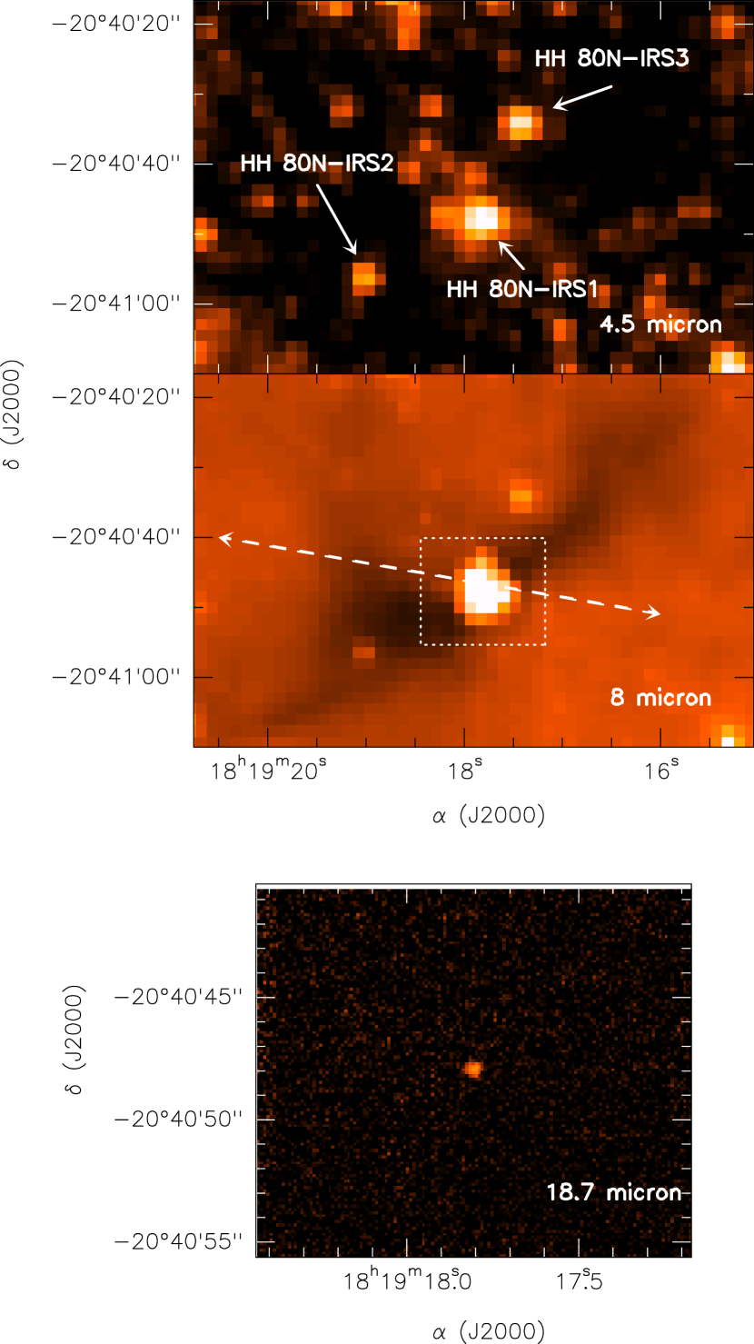
Figure 1: Images of the HH 80N region at 4.5 µm  (top panel) and 8 µm (middle panel), retrieved from the Spitzer archive, and 18.7 µm  (bottom panel) obtained with the VLT. In the middle panel, the dashed square shows the limits of the VISIR (VLT) field of view and the dashed arrow gives approximately the orientation and extend of the outflow detected by Girart et al. 2001.

Ahead of the radio source HH 80N, the obscured northern head of the jet, there is a dense core of $\sim$0.3 pc in size (hereafter HH 80N core) first detected in ammonia (see Fig. 1 of Girart et al. 1994) and afterward in other molecular species (Girart et al. 1998, 2001; Masqué et al. 2009). A comparison between the CS, NH₃ and HCO⁺ emission led Girart et al (1998) to suggest an unusual chemistry for this core. From the ammonia emission of the core a mass of roughly 20 $M_{\odot}$ was estimated by Girart et al. (1994).

Claims for evidence of association of molecular clumps with HH objects have been growing over the last decades (Rudolph & Welch 1988; Davis, Dent & Bell Burnell 1990; Torrelles et al. 1992, 1993; Girart et al.  1994, 1998; 2002, 2005; Viti, Girart & Hatchell 2006; Whyatt et al.  2010). These clumps do not show evidence for shock heating as indicated by their typically observed narrow linewidths (< 1 km s^-1), low temperatures (< 20 K) and radial velocities close to the ambient cloud velocity (e.g. Whyatt et al. 2010). All these properties rule out the possibility of a dynamical perturbation. A possible explanation for the association of molecular clumps with HH objects, proposed by Wolfire & Königl (1992), is that the molecular clump is exposed to a strong UV radiation generated in the HH objects. This radiation is capable of evaporating icy mantles on dust grains, triggering a non-equilibrium chemistry that leads to an increase in abundance of specific molecular species. This scenario was extensively modeled by Taylor & Williams (1996) and Viti & Williams (1999).

In the frame of the photo-illuminated scenario, Girart et al. (1998) suggest that the observed chemistry of the HH 80N core is compatible with the radiative shock-induced chemistry models, being HH 80N the most plausible source of UV irradiation. A more recent study, using several molecular species, appears to be in agreement with this chemical scenario, even though the photochemical effects are observed tentatively only in the side of the core facing HH 80N (Masqué et al. 2009). However, the mass and size of the HH 80N core make this clump quite different from the other molecular clumps found ahead of HH objects. The latter are smaller and less massive (size $\leq$ 0.1 pc; $M\simeq 1~{}M_{\odot}$) than the HH 80N core and do not show any signpost of star formation. Indeed, they are believed to be transient structures or small density fluctuations within the molecular clouds (Viti et al. 2003; Morata et al. 2003, 2005).

Interestingly, Girart et al. (2001) found evidence of a bipolar CO outflow centered near the peak of the HH 80N molecular core, suggesting the presence of an embedded protostar. In addition, Girart et al. (2001) and Masqué et al. (2009) interpreted the distribution and kinematics of CS and other molecular species observed in the outer parts of the HH 80N core as suggestive of an infalling ring-like molecular structure (probably caused by strong molecular depletion in the inner parts) with a radius of $\sim$0.24 pc. The infall velocities inferred ($\sim 0.6$ km s^-1), significantly larger than those expected in the standard protostellar collapse (e.g. ambipolar diffusion models predict gas inward motions of a fraction of the isothermal sound speed, $\sim$0.2 km s^-1, at scales similar those of the HH 80N core; Basu & Moscouvias 1994), led these authors to suggest a peculiar dynamical evolution of this core. Given the particular environment of the HH 80N core, we question whether the HH 80/81/80N outflow has triggered or at least sped up in some way the collapse of the core.

In order to unveil the nature of the HH 80N core, we carried out an extensive set of continuum and ammonia observations over the last years using several instruments, among them VLT and APEX. Using radiative transfer models of collapsing protostellar envelopes, we compare the synthetic spectral energy distribution (SED) and spatial intensity profiles of the dust emission with the data. From this comparison we derive the mass and luminosity of the collapsing envelope, mass infall rate, and mass of the embedded object under the hypothesis that a young stellar object (YSO) is forming inside of the HH 80N core. We explore several density profiles for the initial configuration of the collapsing envelope, and discuss whether the inclusion of an accretion disk is needed to simultaneously explain the observed emission at different wavelengths. Our results point to a new picture for the HH 80N core, which consists in a ’classic’ Class 0 object (hereafter, HH 80N-IRS1) surrounded by a reservoir of material where other clumps potentially forming stars are found.

The paper is organized as follows. In Section 2, we describe the observations. In Section 3 we present the resulting maps. In Section 4 we model the observed dust emission using different approaches for the protostellar collapse. The discussion of the results of the modeling is done in Section 5. Finally, our conclusions are summarized in Section 6.

2 Observations

2.1 VLA

We observed the (J,K) = (1,1) and (2,2) ammonia inversion transitions (at 23.6944955 GHz and 23.7226336 GHz, respectively) using the Very Large Array (VLA) of the NRAO in the D configuration on January 31, 2007. The 4IF spectral correlator mode was used, which allows to observe both transitions in two polarizations simultaneously. The correlator was set to observe a bandwidth of 1.56 MHz with 63 spectral channels of 24.4 kHz (which gives 0.115 km s^-1 of velocity resolution at 1.3 cm) plus a continuum channel that corresponds to 75% of the bandwidth. The phase center of the observations was set to $\alpha(J2000)=18^{\mathrm{h}}19^{\mathrm{m}}18\fs 81$ and $\delta(J2000)=-20\arcdeg 40^{\prime}55\farcs 0$. The flux calibrator was 3C286 with a flux of 2.59 Jy, the phase calibrator was 1832-105 with a bootstrapped flux of $0.88\pm 0.01$ Jy and the bandpass calibrator was 0319+415. Maps of the ammonia (1,1) transition were obtained with natural weighing and using a Gaussian taper of 35 k$\lambda$, which gives a beam size of $6.3\arcsec\times 4.4\arcsec$ (P.A. = 20.0$\arcdeg$) and an rms noise level of $5\times 10^{-3}$ Jy beam^-1 per channel. Here we only present the map of the velocity-integrated flux density of the (1,1) transition, which presents extended emission with a good signal to noise ratio (see § 3.2), for a comparison with the continuum data. A more complete analysis including the ammonia (2,2) transition, that is sensitive to warmer gas, will be presented in a future paper.

2.2 IRAM 30m

The 1.2 mm continuum observations were carried out with the 117-channel bolometer array (MAMBO 2) installed at the 30m IRAM telescope (Pico Veleta, Spain) on January 27 and 28 and March 3, 2008. The data were taken under low sky-noise conditions with the zenith opacity at 250 GHz ranging from 0.14 to 0.28. The on-the-fly technique was used with a scanning speed of $4\arcsec$ s^-1. Chopping was performed with throws of $58\arcsec$ and $70\arcsec$. The angular resolution of the map is $10\farcs 5$ and the achieved rms noise level at this angular resolution is 1.5 mJy beam^-1. Data reduction was carried out with the MOPSIC software.

2.3 Plateau de Bure

The Plateau de Bure Interferometer (PdBI) observations were carried out on April 3 and 10, 2010 in the C configuration. Two tracks were performed under good weather conditions. We made a 6-point mosaic with the phase tracking center of the observations set at $\alpha(J2000)=18^{\mathrm{h}}19^{\mathrm{m}}17\fs 81$ and $\delta(J2000)=-20\arcdeg 40\arcmin 47\farcs 7$, coincident with the Spitzer 8 µm peak position (see § 3.1). The receivers were tuned to the rest frequency of the N₂D (1_1,1–1_0,1) line. The correlator was configured in four widex units (two units for each polarization) that gives a total continuum bandwidth of 8 GHz, plus two narrow windows of 20 kHz covering the N₂D (1_1,1–1_0,1) (85.926263 GHz) and HN¹³C (1–0) (87.090859 GHz) transitions, with a velocity resolution of $\sim 0.15$ km s^-1. The phase calibrator was QSO 1911-201, which has a flux density of 1.09 Jy at the observed frequency, and the flux and bandpass calibrator was MWC349. The data were calibrated using CLIC following the baseline-based mode, since antenna-based solutions were not optimal for the shortest baselines. The continuum map was obtained using MAPPING with natural weighting, that gives a synthesized beam (HPBW) of $7.0\arcsec\times 2.9\arcsec$ (P.A. = $11\arcdeg$) at 86 GHz. The spectral line data will be presented in a future paper.

2.4 VLT

In the nights of May 2 and June 12, 2009, Q-band (20 µm) imaging of the HH 80N region was carried out in service mode using the VISIR instrument installed at the Cassegrain focus of the UT3 telescope (Melipal) of the Very Large Telescope (VLT). The observations covered a field of view of $32.5\arcsec\times 32.5\arcsec$ at a pixel scale of $0.127\arcsec$/pixel.

The sky conditions were good: for the night of May 2 the optical seeing ranged from $0\farcs 8$ to $0\farcs 9$ and the air-mass was $\sim$ 1.05 in average; for the night of June 12 the average optical seeing varied from $1\farcs 0$ to $1\farcs 5$ and the air-mass was always less than 1.05. Under these conditions, the extrapolated seeing at Q band according to the Roddier formula ($\propto\lambda^{0.2}$) is $<0\farcs 5$. Taking into account that the VLT diffraction limit at the same band is $0\farcs 5$, this implies that the angular resolution of our Q band data is basically dominated by diffraction.

During the first observing night our target was observed for one hour through the Q1, Q2, and Q3 filters (covering $17.65\pm 0.83$ µm, $18.72\pm 0.88$ µm, and $19.50\pm 0.40$ $\mu$m, respectively). However, due to the low luminosity of the target, it was not detected in any of these filters. In the second night, our target was observed solely in the Q2 filter for one hour and was detected with a signal-to-noise ratio of 17. In order to remove the atmospheric and telescope background the standard chopping and nodding technique in perpendicular directions was carried out with chop-throws of $14\arcsec$. The standard star for photometric calibration, HD178345 (3.52, 3.15 and 2.88 Jy through Q1, Q2 and Q3 filters, respectively), was observed immediately after our target. A preliminary reduction of the data was carried out using the standard ESO reduction software including the graphical user interface to the pipeline, GASGANO. The final image resulting of shifting and combining the chopping and nodding cycles was obtained with the IRAF package.

The photometric calibration was performed using the ’visir_img_phot’ recipe with the combined image of the cataloged standard star as an input. We obtained conversion factors of 11923.3 (Q1), 11235.0 (Q2, first night), 13379.4 (Q2, second night) and 2446.2 (Q3) between the number of detector counts per second and the source flux in Jy. Q2-band flux density of the target was obtained with standard aperture photometry using the PHOT task of IRAF with a circular aperture of radius $1\farcs 9$ although we inspected values between $1\farcs 5$ and $2\farcs 5$. For the background subtraction, the sky contribution was fitted to an annulus situated between radii of $1\farcs 9$ and $2\farcs 8$ from the center of the aperture. Applying the conversion factor derived above, we obtain a flux density value of 0.175 mJy at 18.7 µm. The flux uncertainty was derived exploring the variation of the flux density value when measured using different apertures.

2.5 APEX

The sub-mm data were obtained with the SABOCA camera, a 39-pixel bolometer array located on the Atacama Pathfinder EXperiment (APEX) telescope in the Chilean Andes. Each SABOCA pixel consists in a composite bolometer with superconducting thermistor on silicon-nitride membranes. The pixels are arranged in a hexagonal layout consisting of a central channel and 3 concentric hexagons. The array is installed at the Cassegrain focus, where it has an effective field of view of $90\arcsec$. SABOCA operates at 850 GHz (350 µm) which gives a beamsize (FWHM) of $7\farcs 7$. The observations were carried out on October 7, 2009 in raster spiral mode with 4 scans, each providing a fully sampled area of $\sim 120\arcsec\times 120\arcsec$. Two skydips, taken in-between and after on-source observations, yielded values of $\sim$ 1.1 for the atmospheric zenith opacity. Pointing was checked on secondary calibrators G10.62, G5.89 and HD-163296.

All the scans were reduced using the miniCRUSH software, a reduced version for the APEX bolometers of the SHARC-2 data reduction package CRUSH. We used the default reduction procedure and the data were smoothed using a $4\farcs 0$ Gaussian that gives an angular resolution of $8\farcs 5$ and an rms noise of 0.09 Jy beam^-1 for the final map.

2.6 Infrared Archive Data from IRAS, Spitzer and Akari

The IRAS Point Source Catalog (PSC) reports a weak source, IRAS 18163-2042, whose position uncertainty includes the HH 80N core. According to the catalog, this source was detected only at 60 $\mu$m with a flux density of $\sim$ 5 Jy and remained undetected in the rest of the bands ($\leq$ 0.5 Jy at 12 and 25 $\mu$m, and $\leq$ 250 Jy at 100 $\mu$m). However, these values are not reliable because of the presence of strong side lobes generated by the nearby luminous source IRAS 18162-2048. These side lobes create a complex background around IRAS 18163-2042, which may cause an underestimate of the flux values reported in the IRAS PSC. This motivated us to SCANPI reprocess the four IRAS bands covering the HH 80N region. SCANPI, a utility provided by the Infrared Processing and Analysis Center (IPAC), performs 1-dimensional scan averaging of the IRAS raw survey data. As it combines all the scans passed over a specific position, its outcome has a higher sensitivity, ideal to obtain fluxes of confused or faint sources. In particular, among all the possible input processing parameters of SCANPI, we gave special attention to the ‘local background fitting range’. By default, an interval of radius $60^{\prime}$ from the scan center is used to fit the background. From this interval, a central range depending on the band is excluded in the fitting in order to prevent contamination from the target: $2^{\prime}$ (12 $\mu$m and 25 $\mu$m), $4^{\prime}$ (60 $\mu$m) and $6^{\prime}$ (100 $\mu$m). Using this default SCANPI yields values similar to the fluxes of the IRAS PSC for all the 1-D scans that pass thorough the HH 80N region. However, IRAS 18162$-$2048 is located $6^{\prime}$ south-east from IRAS 18163$-$2042 and, hence, the default range for the background subtraction includes clearly the emission of this luminous source. Adopting $12^{\prime}$ for the ‘source exclusion range’ in the background fitting for all the bands, we obtained significantly higher flux values than those derived above. Other values for the ‘source exclusion range’ yielded similar results provided that IRAS 18162$-$2048 is excluded from the background fitting range.

To determine better the flux at IRAS bands we checked the Summary Tables in the Result Details page within the SCANPI website. The Summary Tables present single scan data. From this data, we plotted the flux after background subtraction vs. sky offset for each single scan and inspected manually each plot in order to select the scan that showed the best detection. From the selected scan we adopted as the flux value the maximum value of the plot found within the offset interval passing through the target position. We performed this process for all the IRAS bands and obtained new flux values.

We also retrieved observational data of the HH 80N region from the Spitzer archive at 4.5 and 8 µm IRAC bands that are part of a large sample of high-mass star forming regions (PID: 3528). The data at these wavelengths complement very well our VLT observations.

Following the same procedure as for the Q band data, we estimated the flux density at 4.5 and 8 µm with the aperture photometry technique using PHOT of IRAF. We found that significantly larger apertures must be used for the Spitzer data compared to the apertures used for the VLT data: $11\arcsec$ and $12\arcsec$ for and 4.5 and 8 µm images, obtaining flux values of 0.026 and 0.041 Jy for 4.5 and 8 µm, respectively. As for the VLT data, the flux uncertainty was derived by monitoring the variation of the flux value when measured using different apertures.

Finally, we made use of the recently available data from the Infrared Astronomical Satellite Akari. Akari is equipped with two instruments, IRC, covering several bands at near and mid-infrared wavelengths, and FIS, covering several bands at far-infrared wavelengths. From a total of six observable bands, in this paper we present the data of 18, 140 and 160 µm bands. The rest of bands have bad quality data or null detection for our source.

3 Results

3.1 Continuum emission

Figure 1 presents the mid-IR images of the HH 80N region. The Spitzer images at 4.5 and 8 $\mu$m show a bright compact source dominant in the two wavelengths (HH 80N-IRS1). Two other compact sources, located $\sim 20^{\prime\prime}$ South-East (HH 80N-IRS2) and $\sim 15^{\prime\prime}$ North-West (HH 80N-IRS3) of HH 80N-IRS1, may belong to the region. The positions of these compact sources are given in Table 1. HH 80N-IRS1 is also detected in the VLT image at 18.7 µm, but without any extended structure, probably due to the short exposure time of our observations. Taking into account that the source is not resolved, and given the angular resolution of VLT at Q-band ($\sim 0\farcs 5$), the warm part of the envelope remains within $\sim$ 425 AU (for 1.7 kpc of distance) from the core center.

HH 80N-IRS1 is located at the center of the HH 80N core that is seen in absorption against the emission of the Galactic background in the 8 µm image. This observational picture resembles that of InfraRed Dark Clouds (IRDC), being the size of the silhouette of the HH 80N core ($\sim$ 0.4 pc) comparable to the lower limit of the range derived for a sample of IRDCs (0.4-15 pc, Carey et al. 1998). However, while IRDCs harbor the earliest evolutionary stages of high mass star formation (Rathborne et al. 2010), the mass estimated for the HH 80N core (see § 1 and below) seems too low to identify this core as a potential site for the formation of high mass protostars.

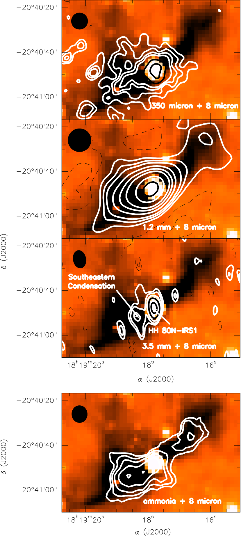
Figure 2: Maps of the HH 80N region taken at 350 µm (top panel), 1.2 mm (second panel), 3.5 mm (third panel) and the velocity integrated (zero-order moment) of the main line of NH₃(1,1) emission (bottom panel), superimposed on the Spitzer 8 $\mu$m image. Contour levels are 3, 4, 6, 9, 15, and 21 times 90 mJy beam^-1 (350 µm); $-$6, $-$3, 3, 6, 9, 15, 21, 27, 39, and 50 times 1.5 mJy beam^-1 (1.2 mm); $-$3, $-$2, 2, 3, 5, 7 and 10 times 0.11 mJy beam^-1 (3.5 mm); 3, 6, 10, 16 and 24 times 0.24 Jy beam^-1 km s^-1(NH₃). The beams are shown in the upper left corner of the panels. The color scale of the infrared image has been modified with respect to Fig. 1 in order to highlight the absorption feature (see text).

As seen in Figure 2, the 350 µm emission is elongated with an angular size of $20\arcsec\times 15\arcsec$ (FWHM) and P.A. $\sim$ 120$\arcdeg$, and peaks at the position of HH 80N-IRS1. Apart from HH 80N-IRS1, the 350 µm emission traces additional material towards the South-East. The 1.2 mm emission peaks at the same position and traces fairly well the silhouette of the absorption feature of the 8 µm image including the north-western tail expanding up to $35\arcsec$ from the central peak. The detection of this tail in emission at 1.2 mm and in absorption at 8 µm excludes the possibility of being an artifact of the 1.2 mm map. In the PdBI 3.5 mm map the dust emission splits into two main sources, one clearly associated with HH 80N-IRS1, plus another southeastern component (hereafter Southeastern Condensation). Table 2 gives the results of Gaussian fits of the 3.5 mm emission for HH 80N-IRS1 and the Southeastern Condensation. In addition, the 3.5 mm map shows two marginally detected sources located $\sim 10\arcsec$ northwest and $\sim 20\arcsec$ southeast of HH 80N-IRS1.

Table 3 gives a summary of the flux density measurements towards HH 80N-IRS1. Since at mm and submm wavelengths it is difficult to discriminate which fraction of the emission of the HH 80N core corresponds to HH 80N-IRS1, in the table we report a range of possible values for the flux densities at these wavelengths. The upper limit of the range at 1.2 mm and 350 µm is an estimate of the HH 80N-IRS1 flux density avoiding the contamination from the Southeastern Condensation. To do this, we integrated the flux density of the western half of the HH 80N core and multiplied the resulting value by 2. The lower limit is the intensity peak that would coincide with the flux density of HH 80N-IRS1 if it were an unresolved source (i.e. the lowest possible contribution). For the 3.5 mm measurement, we take in account the missing short spacings of the PdBI. We made a crude analysis simulating the filtering effects of the $u$-$v$ coverage of our PdBI observations. Using the UVMODEL task of MIRIAD package, we tested these filtering effects on several synthetic maps of artificially generated ellipses that mimic the HH 80N core appearance. We find that a maximum of a 50% of the total flux is missed. Thus, in the range of flux densities given for the 3.5 mm emission, the lower limit corresponds to the flux density measured in the map and the upper limit corresponds to this value corrected by a factor of 2. The data obtained with low angular resolution (i.e. all the IRAS data and the Akari 140 and 160 µm bands) are likely contaminated by background sources. Therefore, we considered these fluxes as upper limits. Finally, note that the complex background of the 8 µm image (see Fig. 1) makes the estimate of the flux at this wavelength somewhat uncertain.

3.2 The nature of NH₃ emission

Figure 2 (bottom panel) presents the NH₃ (1,1) emission superimposed to the Spitzer 8 µm image. The ammonia is very well correlated with the 8 µm absorption feature. It is also well correlated with the 1.2 mm emission. This is not the case for other molecular tracers such as CS or SO presented in previous works (Girart et al. 2001; Masqué et al. 2009), whose emission is significantly more extended ($\sim 60\arcsec\times 25\arcsec$). These studies also show that, in general, the molecular tracers do not peak all at the same position, probably because these molecules are depleted in the densest and inner part of the HH 80N core, that is well traced by the dust continuum emission.

The clear correlation between the NH₃ emission and dust emission indicates that NH₃ traces fairy well the material of the HH 80N core. Girart et al. (2001) detected star forming signatures in the core such as a bipolar outflow traced by CO. In addition, the dust continuum emission shows a compact source, HH 80N-IRS1, in all the observed wavelengths, suggesting the presence of an embedded YSO. All these results suggest that the HH 80N core is currently undergoing active star formation, and that the observed distribution of NH₃ emission arises as a consequence of the high gas densities likely reached in the core, similarly to other star forming cores, and not as a consequence of photochemical effects. Ammonia emission arising as a consequence of a dynamical perturbation is excluded by the narrow NH₃ (1,1) linewidth ($\sim$ 1 km s^-1) observed. Nevertheless, we note that the strongest NH₃ emission is found in the Southeastern part of the core, close to HH 80N, coinciding with the emission detected in the lower sensitivity ammonia observations of Girart et al. (1994). This could be due to a local increment of abundance in this part of the core as found in some species (Masqué et al. 2009); indeed, NH₃ is one of the species predicted to be enhanced by the HH radiation (Viti et al. 2003). Understanding these local departures of the ammonia emission from the global distribution of gas and dust in the HH 80N core is an issue that will require further investigation.

4 Modeling

In the following we analyze this region assuming that an YSO is forming inside the HH 80N core. To do that, we calculate the dust emission arising from an envelope of dust and gas that is collapsing onto a central star. We consider three possible density profiles for the envelope. We first investigate the collapse of a Singular Logatropic Sphere (SLS, McLaughlin & Pudritz 1996; Osorio et al. 1999, 2009). The SLS has a logarithmic relationship between pressure and density, introduced by Lizano & Shu (1989) to empirically take into account the observed turbulent motions in molecular clouds. In the SLS collapse solution an expansion wave moves outward into the static core and sets the gas into motion toward the central star. Outside the radius of the expansion wave the SLS envelope is static, with a dependence of the density with radius as $\rho\propto r^{-1}$. Inside the radius of the expansion wave the gas falls onto the central star with a nearly free-fall behavior ($v\propto r^{-1/2}$, $\rho\propto r^{-3/2}$) at small radii.

As a second approach, we adopt the collapse solution of the Singular Isothermal Sphere (SIS, Shu 1977). In this case the collapse occurs in a similar fashion than in the logatropic case but the radial dependence of the density in the static region goes as $\rho\propto r^{-2}$. Nevertheless, there are important differences in the evolution of both types of collapse as both the speed of the expansion wave and the mass infall rate are constant in the SIS collapse while they increase with time in the SLS collapse.

As a third approach we use the solution for the collapse of a slowly rotating core described in Terebey, Shu and Cassen (1984), hereafter the TSC collapse (see also Cassen & Mossman 1981; Kenyon et al. 1993). In this model, the initial equilibrium state corresponds to the uniformly rotating analogue of the SIS. To first order, the collapse proceeds similarly to the isothermal case beginning at the center of the core and propagating outward at the sound speed as an expansion wave. Material outside the radius of the expansion wave remains in hydrostatic equilibrium (with $\rho\propto r^{-2}$) while inside this radius the infall velocity and density approach those of free fall. However, the angular momentum of the infalling gas becomes important in the vicinity of the centrifugal radius, where motions become significantly non radial and material then falls onto a circumstellar disk rather than radially onto the central object. The centrifugal radius is given by $R_{c}=r_{0}\Omega_{0}/(GM_{*})$, where $\Omega_{0}$ is the angular velocity at a distant reference radius $r_{0}$.

The HH 80N core has a moderate bolometric luminosity, but relatively strong mm and submm emission. By integrating the area below the observed SED, constructed with the flux densities of Table 3, we can derive a possible range of luminosities for HH 80N-IRS1. Considering the lower limits of the mm and submm points and excluding the rest of continuum data in this calculation, we obtain 10 $L_{\odot}$ as the luminosity lower limit. Similarly, taking the upper limits of the mm and submm range and including the 60 µm IRAS point, which is the most restrictive upper limit in the IR part of the SED, we obtain an upper limit of 110 $L_{\odot}$ for the luminosity. We are assuming that the total luminosity, which is responsible for internal heating of the core, is the sum of the stellar luminosity and the infall luminosity caused by the infalling gas onto the protostar. The stellar luminosity can be related to the mass of the central star using the Schaller et al. (1992) evolutionary tracks. The upper limit of the luminosity range deduced above (110 $L_{\odot}$) restricts the mass of the central embedded object to $\leq$ 3 $M_{\odot}$, according to the tables of Schaller et al. (1992); this mass upper limit corresponds to the hypothetical case that all the luminosity of the source was due entirely to the stellar luminosity.

For the SLS and SIS envelopes, the dust temperature is self-consistently calculated from the total luminosity using the dust opacity and the procedures described in Osorio et al. (1999, 2009). These authors calculate the dust opacity at short wavelengths ($\lambda<200$ $\mu$m) assuming that the dust in the envelope is a mixture of graphite, silicates, and water ice, with abundances taken from D’Alessio (1996), and assuming a power law of the form $\kappa_{\lambda}\propto\lambda^{-\beta}$, with $1\leq\beta\leq 2$, for $\lambda\geq 200$ $\mu$m.

The temperature in the TSC case is also self-consistently calculated from the total luminosity, following the procedures described in Calvet et al. (1994) and Osorio et al. (2003). The latter authors obtain the dust opacity over the whole wavelength range assuming a mixture of graphite, silicates and water ice, whose parameters (grain size and abundance) are obtained by fitting the well sampled SED of the prototypical class I object L1551 IRS5.

We computed the SEDs of the models and compared them with the observed values of the flux density of HH 80N-IRS1 (Table 3). Additionally, we produced synthetic maps of the model emission at 3.5 mm, 1.2 mm, and 350 $\mu$m bands. In order to fully simulate the observations, the synthetic maps at 1.2 mm and 350 $\mu$m were convolved with Gaussians with FHWM of $10.5\arcsec$ and $8.5\arcsec$, respectively. For the synthetic map at 3.5 mm, the effect of the missing short spacings of the interferometric observations was taken in account. We used the UVMODEL task of MIRIAD to compute the visibility tables of the 3.5 mm models with the same $u$-$v$ plane coverage as our PdBI observations. Then, from the model visibility tables, we obtained synthetic maps following the standard data reduction routines of the MIRIAD package.

Finally, to check the goodness of our results, we compared selected models with the data by means of spatial intensity profiles obtained using the task CGSLICE of the MIRIAD package, for both the synthetic and observed maps at 1.2 mm, 3.5 mm, and 350 µm. We present two cuts of the observed intensities with P.A. $\simeq 120\arcdeg$ and $\simeq 30\arcdeg$ (mainly along the major and minor axes of the HH 80N core seen at 1.2 mm and 350 µm). An intensity profile obtained with a cut with a selected PA, instead of averaging the emission over an annulus, prevents to include contamination of the Southeastern Condensation. In practice, the synthetic maps of the models in the three approaches have radial symmetry since, in the TSC case, the angular scale of the flattening of the envelope is small enough that it only affects the central pixel of the map. Therefore, for the synthetic maps, we obtained a cut along the diameter of the modeled source.

We explore the SLS and SIS cases separately by running a grid of models taking the mass infall rate ($\dot{M}_{\rm i}$), mass of the central embedded object ($M_{*}$) and the external radius of the core ($R_{\mathrm{ext}}$) as free parameters. Because of the complex morphology of the source (see Fig. 2) we do not adopt a fixed value of $R_{\mathrm{ext}}$; rather, its value is constrained in the fit. The opacity index ($\beta$) was derived to get a trade off to reproduce simultaneously the emission at 1 mm and 350 µm. This yields $\beta\sim 1.6$ for the SLS case and $\beta\sim 1.1$ for the SIS case. For the stellar radius ($R_{*}$) we chose a standard value of 5 $R_{\odot}$ (Schaller et al. 1992). Given the space of parameters ($R_{\mathrm{ext}}$, $\dot{M}_{\rm i}$), we tested values of $M_{*}$ from 0.5 to 1 $M_{\odot}$. Because a fraction of the luminosity is due to infall, higher values of $M_{*}$ would yield luminosities that exceed the upper limit of 110 $L_{\odot}$ derived above, assuming that $\dot{M}_{\rm i}$ $>10^{-5}M_{\odot}$ yr^-1.

The best fit model can be determined by calculating the $\chi^{2}$-statistics obtained from the residual map resulting by subtracting the synthetic from the observed maps. This process was performed for all the sub/mm bands. To find the best fit to the images, we do not include contamination of the Southeastern Condensation in the $\chi^{2}$ analysis. For the 350 µm band, the $\chi^{2}$ function was calculated over a region comprising only the western part of the HH 80N core, roughly a semicircle with a radius of $\sim 20\arcsec$. In the 1.2 mm map, HH 80N-IRS1 cannot be separated from the Southeastern Condensation due to the lower angular resolution of the IRAM 30m observations with respect to the APEX observations. For this case we fit the intensity profile obtained along the minor axis of the emission (i.e. towards NE). For the 3.5 mm map, as HH 80N-IRS1 appears detached from the Southeastern Condensation in the map, a box of $\sim 5\arcsec\times 10\arcsec$ enclosing the entire source was used. Additionally, we calculated the $\chi^{2}$ function for the SED by comparing the fluxes of Table 3 with the predicted SED of the model.

Because the TSC models predict the development of a flattened rotating structure at the innermost part of the envelope, we carried out the modeling assuming a TSC envelope falling onto a disk surrounding the central object. We browsed an appropriate disk model from the online catalog of models of irradiated accretion disks around pre-main sequence stars (D’Alessio et al. 2005). For consistency, the orientation of the disk is chosen to coincide with the rotation axis of the TSC envelope and the disk radius is fixed to the value of the centrifugal radius $R_{c}$. To obtain the SED of the total composite model, we added the fluxes of the disk and envelope at each wavelength accounting for the extinction of the envelope, which is important at short wavelengths. Since the disk is unresolved even in the images with the highest angular resolution, to obtain the synthetic maps we added the disk to the envelope as a point source at the central pixel.

Due to computational limitations, the fitting process of the TSC envelope plus circumstellar disk could not be automated. Our strategy, then, was to perform a case-by-case exploration varying the external radius of the core ($R_{\mathrm{ext}}$), the radius of the expansion wave ($R_{\mathrm{ew}}$), and the reference density ($\rho_{1}$) (this latter parameter is the density the envelope would have at a radius of 1 AU for the limit $R_{c}=0$, and it is related to the mass infall rate and the central mass through equation 3 of Kenyon et al. 1993), until we found a model that explains satisfactorily the SED and the intensity profile at 350 µm, 1.2 mm and 3.5 mm. The caveat of this method is that there is no assurance of finding a unique best fit model. However, the goal of this section is to prove that the observed properties of the continuum emission observed in the HH 80N core can be explained in terms of a protostar plus an infalling envelope that is embedded inside the HH 80N core. Constraining a unique model with a flattened envelope and a disk requires additional mid-IR observations with high angular resolution and it is beyond the scope of this paper.

4.1 Results for the SLS model

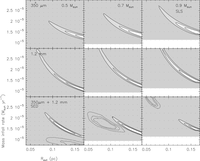
Figure 3: Contour plots (solid line and gray scale) of the $\chi^{2}$ function derived for the fitting of the models of the collapse of the Singular Logatropic Sphere to the observed images. Rows correspond to the 350 µm band (top), the 1.2 mm band (middle), and the sum of the $\chi^{2}$ function for the 350 µm and 1.2 mm bands (bottom). The dotted contours shown in the bottom panels correspond to the $\chi^{2}$ function derived for the SED. Columns correspond to $M_{*}$ = 0.5 $M_{\odot}$ (left), 0.7 $M_{\odot}$ (middle), and 0.9 $M_{\odot}$ (right). In all the cases the contour levels correspond to the confidence levels of 99%, 90% and 68% (1$\sigma$). These contours are relative to the minimum $\chi^{2}$ value of each panel, which may vary significantly for different masses. For instance, in the bottom row, where we compare the results of the SED and single-dish maps, the minimum $\chi^{2}$ values of the SED are 53.4, 33.2, and 19.2 for 0.5, 0.7, and 0.9 $M_{\odot}$, respectively; the sum of the minimum $\chi^{2}$ values of the 350 µm and 1.2 mm maps are 102.2, 119.0, and 122.2 for 0.5, 0.7, and 0.9 $M_{\odot}$, respectively.

We tested the logatropic density distribution by using 1080 different models within the following set of ranges for the external radius, mass infall rate and mass of the central embedded object: 0.04 pc $\leq$ $R_{\mathrm{ext}}$  $\leq$ 0.18 pc, $7\times 10^{-6}M_{\odot}$ yr${}^{-1}\leq$ $\dot{M}_{\rm i}$ $\leq 5\times 10^{-5}M_{\odot}$ yr^-1 and 0.5 $M_{\odot}$ $\leq$ $M_{*}$ $\leq$ 1.0  $M_{\odot}$. In this space of parameters we expect to find meaningful physical solutions. To establish the goodness of the fit we calculated the $\chi^{2}$ as discussed in the previous section. Figure 3 shows the best set of solutions for the $\chi^{2}$ estimated separately for the SED and for the 1.2 mm and 350 µm intensity distributions. We also calculated the $\chi^{2}$ function for the 3.5 mm band but the results are not included in the figure because no set of parameters can provide reasonable $\chi^{2}$ values at this band. We consider as good solutions those where the $\chi^{2}$ values of the intensity distributions and of the SED are all within the 90% level of confidence.

Figure 3 shows that there are no solutions that fit together the SED and the intensity distribution of the 1.2 mm and 350 $\mu$m maps (i.e., there is no overlap between the $\chi^{2}$ contours of the maps and those of the SED). As an example, Figures 4 and 5 show, respectively, the predicted SED and intensity profiles (dash-dotted lines) of the SLS model that gives the minimum $\chi^{2}$ for the SED, compared with the observed data. Except for the mid-IR wavelengths, the observed SED is reasonably well reproduced by the model. However, as Figure 5 shows, this model produces intensity profiles too flat and cannot reproduce the observed intensity profiles in any of the bands. Given these discrepancies, we conclude that in the logatropic case the mass is not distributed adequately in the envelope to match the observations.

4.2 Results for the SIS model

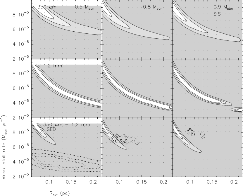
Figure 6: Contour plots (solid line and gray scale) of the $\chi^{2}$ function derived for the fitting of the models of the collapse of the Singular Isothermal Sphere to the observed images of HH 80N-IRS1. Rows correspond to the 350 µm band (top), the 1.2 mm band (middle), and the sum of the $\chi^{2}$ function for the 350 µm and 1.2 mm bands (bottom). The dotted contours shown in the bottom panels correspond to the $\chi^{2}$ function derived for the SED. Columns correspond to $M_{*}$ = 0.5 $M_{\odot}$ (left), 0.8 $M_{\odot}$ (middle), and 0.9 $M_{\odot}$ (right). In all the cases the contour levels correspond to the confidence levels of 99%, 90% and 68% (1$\sigma$). These contours are relative to the minimum $\chi^{2}$ value of each panel, which may vary significantly for different masses. For instance, in the bottom row, where we compare the results of the SED and single-dish maps, the minimum $\chi^{2}$ values of the SED are 47.1, 278.6, and 600.3 for 0.5, 0.7, and 0.9 $M_{\odot}$, respectively; the sum of the minimum $\chi^{2}$ values of the 350 µm and 1.2 mm maps are 40.6, 36.1, and 36.7 for 0.5, 0.7, and 0.9 $M_{\odot}$, respectively.

We tested the isothermal density distribution by using 1800 different models within the following set of ranges for external radius, mass infall rate and mass of the central embedded object: 0.03 pc $\leq$ $R_{\mathrm{ext}}$$\leq$ 0.22 pc, $1.2\times 10^{-5}M_{\odot}$ yr${}^{-1}\leq$ $\dot{M}_{\rm i}$ $\leq 1.6\times 10^{-4}M_{\odot}$ yr^-1 and 0.5 $M_{\odot}$ $\leq$ $M_{*}$ $\leq$ 1.0  $M_{\odot}$. Figure 6 shows the best models from the $\chi^{2}$ analysis for the SIS case. For the same reasons as in the logatropic case, we have not included the 3.5 mm results in the figure.

The mass infall rates considered for the SIS collapse are higher than those considered in the logatropic case. This is because, for a given value of the mass infall rate, the SIS models yield less massive envelopes than the SLS models; so, in order to fit properly the mm flux densities higher values of the mass infall rate are required in the SIS models (see Osorio et al. 1999). For this reason, $R_{\mathrm{ext}}$ becomes almost irrelevant and $\dot{M}_{\rm i}$ takes the dominant role in the fitting. Figure 6 (bottom panels) shows that for the $M_{*}$ $=0.8$ $M_{\odot}$ case, there are solutions that apparently satisfy both the SED and (sub)mm intensity distribution constraints (i.e., for 0.8 $M_{\odot}$, the $\chi^{2}$  contours of the SED overlap those of the maps for $R_{\mathrm{ext}}$ $\simeq$ 0.08-0.1 pc and $\dot{M}_{\rm i}$ = (6.5-8.0)$\times 10^{-5}~{}M_{\odot}$ yr^-1). Nevertheless, despite these solutions yielding reasonable intensity distributions in the 1.2 mm and 350 µm  bands, they overestimate the total luminosity, specially at far-IR wavelengths. In Figure 4 (dashed line) we show an example that illustrates this behavior (the predicted flux is almost one order of magnitude above the observed flux at 60 µm). As in the SLS case, the modeled intensity profile at 3.5 mm (dashed line in Fig. 5) is significantly weaker than the observed profile. These results are general and we can find solutions that can fit the single–dish intensity distribution of the envelope but they predict an excess of luminosity and fail to reproduce the compact emission seen in the 3.5 mm PdBI map. In conclusion, as in the SLS case, there is no SIS model that can fit the SED and the maps simultaneously.

4.3 Results for the TSC model

One of the caveats of the SLS and SIS models is that they are unable to fit the intensity of the compact source seen in the PdBI 3.5 mm map. This compact source could have a significant contribution from a circumstellar disk. In this section we model the source assuming a TSC envelope falling onto a disk surrounding the central object obtained from the catalog of D’Alessio et al. (2005). Apart from using a more realistic model, such a configuration is ideal for two reasons. First, if the circumstellar disk is populated by millimeter-size grains, its emission can be significant at mm wavelengths and, because it is compact, it will be less affected by the interferometric filtering that affects the envelope emission. Second, because the SED at short wavelengths is very sensitive to the geometry of the source, the TSC envelope and a disk with the proper inclination can provide the extinction required to fit the mid-IR part of the SED, depending on the inclination of the axis of the system (envelope plus disk). This would give luminosities similar to or below 110 $L_{\odot}$. In addition, the infall luminosity is reduced because the material lands on a disk instead of falling directly onto the protostar.

We tested several TSC envelopes exploring values of the central luminosity $50<L_{*}<250$ $L_{\odot}$, outer radius of the envelope $0.07<R_{\rm ext}<0.18$ pc, the radius of the expansion wave $0.03<R_{\rm ew}<0.09$ pc, and reference density $4.1\times 10^{-13}<\rho_{1}<1\times 10^{-12}$ g cm^-3 (these values of $\rho_{1}$ are equivalent to densities at 1000 AU between $7.8\times 10^{5}$ and $7.4\times 10^{6}$ cm^-3, and correspond to values of the mass infall rate between $3.2\times 10^{-5}$ and $3.3\times 10^{-4}~{}M_{\odot}$ yr^-1 for a 3 $M_{\odot}$ star). For the circumstellar disk we explored accretion rates from the disk to protostar between $10^{-9}$ to $10^{-6}M_{\odot}$ yr^-1, and we assume that the disk is irradiated with a similar luminosity and has a similar inclination than the envelope. In Table 4 we give the parameters of our favored model. Figures 7 and 8 show the observed SED and intensity profiles, respectively, predicted by our favored TSC model. These figures show that the SED is well reproduced by the model in almost all the data points and that the modeled intensity profiles fit reasonably well the observations within the calibration uncertainties.

At 3.5 mm, the inclusion of a disk provides the flux needed to explain the observed intensity peak. We note that, possibly, a fine tuning of the mass accretion rate could provide a more accurate fit for the intensity profiles. However, the range of accretion rates of the online disk model grid is sampled in steps that vary one order of magnitude and the next available model has an accretion rate too small and provides too faint mm emission. Nevertheless, in this analysis we aimed to prove that our continuum observations can be explained in the frame of standard star forming models and our favored model presented above fulfills this requirement. Table 5 shows a summary of the $\chi^{2}$ analysis (SED, single-dish and interferometric maps) for this TSC (+disk) model (Figs. 7, 8), as well as for the SLS and SIS models shown in Figures 4, 5. The reduced $\chi^{2}$ values show that in the TSC case we obtain a better fit.

5 Discussion

The derived physical parameters of the selected TSC model listed in Table 4 suggest that HH 80N-IRS1 is a very young Class 0 protostar. First, the predicted volume density for HH 80N-IRS1 at 1000 AU, $n({\rm H_{2}})\simeq 4\times 10^{6}$ cm^-3, is typical of Class 0 sources (Jørgensen et al. 2002), and greater than Class I sources (Jørgensen et al. 2002) and prestellar cores (Kirk, Ward-Thomson & André 2005; Tafalla et al. 2002); second, the estimated upper limit of the mass infall rate, $\sim 2\times 10^{-4}M_{\odot}$ yr^-1 (see Table 4), is compatible with the high values of the mass infall rate typical of young Class 0 protostars (Maret et al. 2002), and yields to an age of $\sim 2\times 10^{4}$ yr for HH 80N-IRS1; finally, HH 80N-IRS1 fulfills the criteria proposed by André et al. (1993) for Class 0 objects, $L_{\rm submm}/L_{\rm bol}\gtrsim 5\times 10^{-3}$, which in our case is about 0.1. On the other hand, the derived luminosity of 105 $L_{\odot}$ for HH 80N-IRS1 is found in the threshold between low mass and intermediate mass protostars. Given the large reservoir of mass of the HH 80N core (see 1.2 mm and 350 µm map of Fig. 2) and the youth of the HH 80N-IRS1, we cannot discard further accumulation of material towards the central object.

From the integrated emission of the residual map at 1.2 mm (resulting from the subtraction of the emission of the synthetic map of the TSC model from the map observed with MAMBO) we can obtain a crude estimate of the mass of the HH 80N core outside the HH 80N-IRS1 envelope. Assuming optically thin dust emission with $\beta=2$ and a temperature of $\sim$14 K (the boundary temperature of the HH 80N-IRS1 envelope) we derive a mass of $\sim$10 $M_{\odot}$ for this material. As we noted above, the HH 80N core, with a size of $0.16\times 0.12$ pc and an estimated total mass of $\sim$30 $M_{\odot}$ (20 $M_{\odot}$ of HH 80N-IRS1 + 10 $M_{\odot}$ of the rest of the HH 80N core), contains more material than the infalling envelope associated with IRS1. According to the results of our TSC modeling (see Table 4) the mass of the envelope is 20 $M_{\odot}$, and the infall occurs within a radius of $R_{\mathrm{ew}}$ = $1.5\times 10^{4}$ AU with the envelope being static outside this radius. Furthermore, the molecular emission of tracers such CS, SO and HCO⁺ extends over a region considerably larger than the HH 80N core, as traced by the dust continuum and ammonia line emissions. Indeed, the emission of these molecular tracers has been interpreted as arising from a contracting ring around HH 80N-IRS1 with an inner radius (the radius of the region where these molecular species appear to be depleted) of $2.5\times 10^{4}$ AU and an outer radius of $6\times 10^{4}$ AU (Girart et al. 2001; Masqué et al. 2009). The estimated average volume density of the molecular ring is in the $5\times 10^{4}$-$1.3\times 10^{5}$ cm^-3 range (Masqué et al. 2009), which seems too high, given the estimated density in the static part of the HH 80N-IRS1 envelope ($\sim 6\times 10^{4}$ cm^-3, according to our modeling). Therefore, the kinematics and physical conditions in the molecular ring-like structure proposed by Girart et al. (2001) and Masqué et al. (2009) appear puzzling. The role of the HH 80/81/80N outflow in the properties of this molecular ring-like structure and the relationship with the onset of the star-forming process in the HH 80N core, in particular with the HH 80N-IRS1, protostar is an interesting issue that deserves further observational and theoretical investigation.

6 Conclusions

We have carried out dust continuum and ammonia line observations of the dense core ahead of HH 80N, complemented with archive data, covering a wide range of wavelengths. We analyzed the continuum data by means of self-consistent models using several approaches for the envelope structure and we discuss the inclusion of a protostellar disk. Additionally, we compare ammonia observations of the (1,1) transition with continuum emission (and absorption) maps. Our main conclusions are summarized as follows:

1. The NH₃ (1,1) emission shows a striking correlation with the dust continuum emission and with the absorption silhouette seen in the 8 µm  Spitzer image. This indicates that the ammonia traces fairly well the distribution of gas and dust in the HH 80N core. Pending a proper analysis of the NH₃ abundances, this preliminary assessment points that there is no need to invoke photochemical effects caused by the nearby HH 80N object to explain the distribution of ammonia in the HH 80N core. However, a detailed inspection of the ammonia map shows that an important part of the NH₃ emission arises from the Southeastern part of the core, close to HH 80N, which could be due to a slight abundance enhancement.

2. The continuum emission presents a peak at the same position ($\alpha(J2000)=18^{\mathrm{h}}19^{\mathrm{m}}17\fs 81$, $\delta(J2000)=-20\arcdeg 40^{\prime}47\farcs 7$) in all the bands (4.5 µm, 8 µm, 350 µm, 1.2 mm and 3.5 mm). This emission peak is located at the center of the CO bipolar outflow found by Girart et al. (2001), suggesting the presence at this position of an embedded young stellar object (HH 80N-IRS1) that powers the outflow.

3. We find that the SED and the intensity distribution of the mm and submm emission of HH 80N-IRS1 can be reproduced by a slowly rotating infalling envelope described by the Terebey, Shu, and Cassen (TSC) solution, plus a circumstellar accretion disk. The mass of the envelope is 20 $M_{\odot}$, the central luminosity is 105 $L_{\odot}$, and the radius of the infalling region is 1.5$\times 10^{4}$ AU. The disk has a mass of 0.6 $M_{\odot}$ and a radius of 300 AU. Such a configuration, together with the derived high values of the mass infall rate ($1.7\times 10^{-4}\,(M_{*}/3\,M_{\odot})^{1/2}~{}M_{\odot}$ yr^-1), and young age ($\sim 2\times 10^{4}$ yr), suggest the HH 80N-IRS1 may be a young Class 0 source.

4. The APEX map at 350 µm and, especially, the PdBI map at 3.5 mm, where the extended emission is resolved out, show signs of possible fragmentation suggesting that other sources, in addition to HH 80N-IRS1, could be embedded inside the HH 80N core. On the other hand, previous studies reveal that the molecular emission of some tracers is considerably more extended than the dust and NH₃ emission presented in this work. This suggests that the HH 80N core is surrounded by a larger molecular structure whose properties could be influenced by the proximity of the HH 80/81/80N outflow.

Figure 4: Observed flux densities (dots; see Table 3) and predicted SEDs for HH 80N-IRS1, assuming models of the collapse of the Singular Logatropic Sphere (SLS; dash-dotted line) and of the Singular Isothermal Sphere (SIS; dashed line). Bars represent the uncertainties and arrows represent upper limits. The SLS model corresponds to the model that minimizes the $\chi^{2}$ of the SED ($R_{\mathrm{ext}}$ = 0.1 pc, $M_{*}$= 0.7 $M_{\odot}$, $\dot{M}_{\rm i}$= 1.57 $\times 10^{-5}~{}M_{\odot}$ yr^-1, $L_{\mathrm{bol}}=69$ $L_{\odot}$, $M_{\mathrm{env}}=25.5$ $M_{\odot}$, and $\beta$ = 1.6). The SIS model corresponds to the model that minimizes the $\chi^{2}$ function for the maps at 1.2 mm and 350 µm ($R_{\mathrm{ext}}$ = 0.05 pc, $M_{*}$ = 0.8 $M_{\odot}$, $\dot{M}_{\rm i}$ = 1.05 $\times 10^{-4}M_{\odot}$ yr^-1, $L_{\mathrm{bol}}=527$ $L_{\odot}$, $M_{\mathrm{env}}=4.6$ $M_{\odot}$, and $\beta$ = 1.1).

Figure 5: Observed and modeled intensity profiles of HH 80N-IRS1 at 350 µm (top), 1.2 mm (middle) and 3 mm (bottom). The squares and triangles represent observed cuts along the major (P. A. $\simeq 120\arcdeg$) and minor (P. A. $\simeq 30\arcdeg$) axes of the HH 80N core, respectively. Bars represent the uncertainties. At 3.5 mm, as the source appears unresolved, we present only a cut along the major axis of the core (P. A. $\simeq 120\arcdeg$). The dash-dotted lines correspond to cuts along the diameter of the synthetic maps of the Singular Logatropic Sphere model that minimizes the $\chi^{2}$ for the SED (see Fig. 4). The dashed lines correspond to cuts along the diameter of the synthetic maps of the Singular Isothermal Sphere model that minimizes the $\chi^{2}$ for the maps (see Fig. 4). The dotted line represents the beam.

Figure 7: Observed flux densities (dots; see Table 3) and predicted SED for HH 80N-IRS1, assuming the Terebey, Shu, and Cassen (TSC) envelope model plus an accretion disk. Bars represent the uncertainties and arrows represent upper limits. The dashed line represents the SED of our favored TSC envelope model ($R_{\rm ext}=1.8\times 10^{4}$ AU, $M_{*}$= 3 $M_{\odot}$, $\dot{M}_{\rm i}$ $\simeq 1.6\times 10^{-4}M_{\odot}$ yr^-1, $L_{\mathrm{bol}}=105$ $L_{\odot}$, and $M_{\mathrm{env}}=20$ $M_{\odot}$). The point dashed line represents the SED of the selected disk model ($\dot{M}_{\rm acc}$ $=10^{-7}M_{\odot}$ yr^-1, $R_{c}=$ 300 AU, and $i=30\arcdeg$). The solid line represents the resulting SED of out favored TSC envelope plus disk model.

Figure 8: Observed and modeled intensity profiles of HH 80N-IRS1 at 350 µm (top), 1.2 mm (middle) and 3 mm (bottom). The squares and triangles represent observed cuts along the major (P. A. $\sim 120\arcdeg$) and minor (P. A. $\sim 30\arcdeg$) axes of the HH 80N core, respectively. Bars represent the uncertainties. At 3.5 mm, as the source appears unresolved, we present only a cut along the major axis of the core (P. A. $\sim 120\arcdeg$). The solid lines correspond to cuts along the diameter of the synthetic maps of our favored Terebey, Shu, and Cassen envelope plus disk model (see Fig. 7). The dotted line represents the beam.

Table 1: Positions of the compact Spitzer sources

	Peak Position
Source	RA(J2000)	DEC (J2000)
HH 80N-IRS1	$18^{\mathrm{h}}19^{\mathrm{m}}17\fs 81$	$-20\arcdeg 40^{\prime}47\farcs 7$
HH 80N-IRS2	$18^{\mathrm{h}}19^{\mathrm{m}}19\fs 01$	$-20\arcdeg 40^{\prime}56\farcs 4$
HH 80N-IRS3	$18^{\mathrm{h}}19^{\mathrm{m}}17\fs 42$	$-20\arcdeg 40^{\prime}34\farcs 3$

Table 2: Source parameters derived from the PdBI 3.5 mm map

	Peak Position		$I_{\nu}$(peak)	$S_{\nu}$	Deconvolved Size	P. A.
Source	RA(J2000)	DEC (J2000)	(mJy beam-1)	(mJy)	($\arcsec$)	($\arcdeg$)
HH 80N-IRS1	$18^{\mathrm{h}}19^{\mathrm{m}}17\fs 81$	$-20\arcdeg 40^{\prime}47\farcs 7$	$2.03\pm 0.11$	$3.75\pm 0.19$	$5.0\times 3.0$	-17.4
Southeastern Condensation	$18^{\mathrm{h}}19^{\mathrm{m}}18\fs 31$	$-20\arcdeg 40^{\prime}52\farcs 2$	$0.58\pm 0.06$	$2.48\pm 0.09$	$11.1\times 5.8$	-17.0

Table 3: Summary of the continuum data of HH 80N-IRS1

		Angular	Aperture	Flux
Wavelength		Resolution	Size	Density	Observing
($\mu$m)	Instrument	($\arcsec$)	($\arcsec$)	(Jy)	Epoch	Notes
3500	IRAM PdBI	2.9 $\times$ 7.0	$\sim 5\times 10$	0.004–0.006	April 2010	This paper
1200	IRAM 30m (MAMBO II)	10.5		0.084–0.177	March 2008	This paper
350	APEX (SABOCA)	8.5	$\sim 30\times 50$	2.1–5.9	October 2009	This paper
160	Akari (FIS)	$\sim$ 60	–	$\leq$ 33.88	2006-2007	Archive data
140	Akari (FIS)	$\sim$ 55	–	$\leq$ 36.11	2006-2007	Archive data
100	IRAS	180 $\times$ 300	–	$\leq$ 108	1983	Archive data
60	IRAS	90 $\times$ 282	–	$\leq$ 22.08	1983	Archive data
25	IRAS	45 $\times$ 276	–	$\leq$ 1.24	1983	Archive data
18.7	VLT (VISIR)	$\sim 0.5$	1.5	0.175 (0.01)	June 2009	This paper
18.0	Akari (IRC)	$\sim$ 7	–	0.170 (0.009)	2006-2007	Archive data
12	IRAS	45 $\times$ 270	–	$\leq$ 0.46	1983	Archive data
8	Spitzer (IRAC)	1.7	12	0.041 (0.010)	September 2005	Archive data
4.5	Spitzer (IRAC)	1.9	11	0.026 (0.003)	September 2005	Archive data

Table 4: Results of the TSC modeling

Envelope parameter	Symbol	Value
Mass	$M$	20 $M_{\odot}$
Central luminosity	$L_{*}$	105 $L_{\odot}$
Radius of the expansion wave	$R_{\rm ew}$	$1.5\times 10^{4}$ AU
Outer radius	$R_{\rm ext}$	$1.8\times 10^{4}$ AU
Inclination angle	$i$	30$\arcdeg$
Centrifugal radius	$R_{c}$	300 AU
Reference density	$\rho_{1}$	$5\times 10^{-13}$ gr cm-3
Density at $r=1000$ AU	$n$ (1000 AU)	$4.1\times 10^{6}$ cm-3
Mass infall rate	$\dot{M}_{\rm i}$	$1.6\times 10^{-4}M_{\odot}$ yr-1
Disk parameter	Symbol	Value
Mass	$M_{\rm disk}$	0.6 $M_{\odot}$
Radius	$R_{\rm disk}$	300 AU
Inclination angle	$i$	30$\arcdeg$
Mass accretion rate	$\dot{M}_{\rm acc}$	$10^{-7}M_{\odot}$ yr-1
Viscosity parametrization	$\alpha$	0.01
Slope of grain size distribution	p	3.5
Minimum grain size	$a_{\rm min}$	0.005 µm
Maximum grain size	$a_{\rm max}$	1 mm

Table 5: Reduced $\chi^{2}$ Results

		Single-dish	Interferometric
	SED	maps	map
SLS model	34.1	31.5	68.3
SIS model	441.4	3.3	13.3
TSC+disk model	3.5	8.1	5.5

References

- (1)
- (2) André, P., Ward-Thompson, D., & Barsoni, M. 1993, ApJ, 406, 122
- (3) Basu, S., & Mouschovias, T, Ch. 1994, ApJ, 432, 720
- (4) Calvet, N., Hartmann, L., Kenyon, S. J.,& Whitney, B. A. 1994, ApJ, 434, 330
- (5) Carey, S. J., Clark, F. O., Egan, M. P., Price, S. D., Shipman, R. F., & Kuchar, T. A. 1998, ApJ, 508, 721
- (6) Carrasco-González, C., Rodríguez, L.F., Anglada, G., Martí, J., Torrelles, J.M., & Osorio, M., 2010, Science, 330, 1209
- (7) Cassen, P., Mosman, A. 1981 Icarus, 48, 353
- (8) D’Alessio, P., 1996, PhD. thesis
- (9) D’Alessio, P., Merín, B., Calvet, N., Hartmann, L., & Montesinos, B. 2005, Rev. Mexicana Astron. Astrofis., 41, 61
- (10) Davis, C. J., Dent, W. R. F, & Bell Burnell, S. J. 1990, MNRAS, 244, 173
- (11) Fernández-López, M., Curiel, S., Girart, J. M., Ho, P. T. P., Patel, N., & Gómez, Y. 2011, AJ, 141, 72
- (12) Girart, J. M., et al. 1994, ApJ, 435, L145
- (13) Girart, J. M., Estalella, R. , & Ho, P. T. P. 1998, ApJ, 495, L59
- (14) Girart, J. M., Estalella, R., Viti, S., Williams, D. A., & Ho, P. T. P. 2001, ApJ, 562, L91
- (15) Girart, J. M., Viti, S., Williams, D. A., Estalella, R., & Ho, P. T. P. 2002, A&A, 388, 1004
- (16) Girart, J. M., Viti, S., Estalella, & Williams, D. A. 2005, A&A, 439, 601
- (17) Gyulbudaghian, A. L., Glushkov, Y. I., & Denisyuk, E. K. 1978, ApJ, 224, 137
- (18) Jørgensen, J. K., Schöier, F. L., & van Dishoeck, E. F. 2002, A&A, 389, 908
- (19) Kenyon, S. J., Calvet, N., & Hartmann, L. 1993, ApJ, 414, 676
- (20) Kirk, J. M., Ward-Thomson, D., & André, P. 2005, MNRAS, 360, 1506
- (21) Lizano, S., & Shu, F. H. 1989, ApJ, 342, 834
- (22) Martí, J., Rodríguez, L.F., & Reipurth, B. 1993, ApJ, 416, 208
- (23) Masqué, J. M., Girart, J. M., Beltrán, M. T., Estalella, R., & Viti, S. 2009, ApJ, 695, 1505
- (24) Maret, S., Ceccarelli, C., Caux, E., Tielens, A. G. G. M., & Castets, A. 2002, A&A, 395, 573
- (25) McLaughlin, D. E., & Pudritz, R. E. 1996, AAS, 189, 1503
- (26) Molinari, S., Noriega-Crespo, A., & Spinoglio, L. 2001, ApJ, 547, 292
- (27) Morata, O., Girart J. M., & Estalella, R., 2003 A&A, 397, 181
- (28) Morata, O., Girart J. M., & Estalella, R., 2005 A&A, 435, 113
- (29) Osorio, M., Lizano, S., & D’Alessio, P. 1999, ApJ, 525, 808
- (30) Osorio, M., D’Alessio, P., Muzerolle, J., Calvet, N., & Hartmann, L. 2003, ApJ, 586, 1148
- (31) Osorio, M., Anglada, G., Lizano, S., & D’Alessio, P. 2009, ApJ, 649, 29
- (32) Rathborne, J. M., Jackson, J. M., Chambers, E. T., Stojimirovic, I., Simon, R., Shipman, R., & Frieswijk, W. 2010, ApJ, 715, 310
- (33) Rodríguez, L. F., Moran, J. M., Gottlieb, E. W., & Ho, P. T. P. 1980, ApJ, 235, 845
- (34) Rudolph, A., & Welch, W. J. 1988, ApJ, 326, L31
- (35) Schaller, G., Schaerer, D., Meynet, G., Maeder, A. 1992, A&AS, 96, 269
- (36) Shu, F. H., Adams, F. C., & Lizano, S. 1987, ARA&A, 25, 23
- (37) Tafalla, M., Myers, P. C., Caselli, P., Walmsley, C. M., & Comito, C. 2002, ApJ, 569, 815
- (38) Taylor, S.D., & Williams, D.A. 1996, MNRAS, 282, 1343
- (39) Terebey, S., Shu, F. H., & Cassen, P. 1984, ApJ, 286, 529
- (40) Torrelles, J. M., Rodríguez, L. F., Cantó, J., Anglada, G., Gómez J. F., Curiel, S., & Ho, P. T. P. 1992, ApJ, 396, L95
- (41) Torrelles, J. M., Gómez, J. F., Ho, P. T. P., Anglada, G., Rodríguez, L. F., & Cantó, J. 1993, ApJ, 417, 655
- (42) Viti, S., & Williams, D. A. 1999, MNRAS, 310, 517
- (43) Viti, S., Girart, J. M., Garrod, R., Williams, D. A., & Estalella, R. 2003, A&A, 399, 187
- (44) Viti, S., Girart, J. M., & Williams, D. A. 2006, A&A, 449, 1089
- (45) Whyatt, W., Girart, J. M., Viti, S., Estalella, R., & Williams, D. A. 2010, A&A, 510, 74
- (46) Wolfire, M. G., & Königl, A. 1993, ApJ, 415, 204
- (47)