Revealing the “missing” low-mass stars in the S254-S258 star forming region by deep X-ray imaging

Abstract

Context. X-ray observations provide a very good way to reveal the population of young stars in star forming regions avoiding the biases introduced when selecting samples based on infrared excess.

Aims. The aim of this study was to find an explanation for the remarkable morphology of the central part of the S254–S258 star forming complex, where a dense embedded cluster of very young stellar objects (S255-IR) is sandwiched between the two H II regions S255 and S257. This interesting configuration had led to different speculations such as dynamical ejection of the B-stars from the central cluster or triggered star formation in a cloud that was swept up in the collision zone between the two expanding H II regions. The presence or absence, and the spatial distribution of low-mass stars associated with these B-stars can discriminate between the possible scenarios.

Methods. We performed a deep Chandra X-ray observation of the S254–S258 region in order to efficiently discriminate young stars (with and without circumstellar matter) from the numerous older field stars in the area.

Results. We detected 364 X-ray point sources in a $17^{\prime}\times 17^{\prime}$ field ($\approx 8\times 8$ pc). This X-ray catalog provides, for the first time, a complete sample of all young stars in the region down to $\sim 0.5\,M_{\odot}$. A clustering analysis identifies three significant clusters: the central embedded cluster S255-IR and two smaller clusterings in S256 and S258. Sixty-four X-ray sources can be classified as members in one of these clusters. After accounting for X-ray background contaminants, this implies that about 250 X-ray sources constitute a widely scattered population of young stars, distributed over the full field-of-view of our X-ray image. This distributed young stellar population is considerably larger than the previously known number of non-clustered young stars selected by infrared excesses. Comparison of the X-ray luminosity function with that of the Orion Nebula Cluster suggests a total population of $\sim 2000$ young stars in the observed part of the S254-S258 region.

Conclusions. The observed number of $\sim 250$ X-ray detected distributed young stars agrees well with the expectation for the low-mass population associated to the B-stars in S255 and S257 as predicted by an IMF extrapolation. These results are consistent with the scenario that these two B-stars represent an earlier stellar population and that their expanding H II regions have swept up the central cloud and trigger star formation (i.e. the central embedded cluster S255-IR) therein.

1 Introduction

1.1 The S254-S258 complex

The south-eastern part of the molecular cloud complex in the Gem OB1 association contains an embedded star-forming region with several diffuse H II regions (S254–S258, Sharpless 1959, see Fig. 1). The most prominent of these H II regions, S255 and S257 (Chopinet et al., 1974), are both powered by B0 stars, have diameters of $\sim 4^{\prime}$, and a projected separation of $\sim 6^{\prime}$. Sandwiched right between them is a dense dusty molecular cloud filament (S255-IR or S255-2; Heyer et al. 1989; Di Francesco et al. 2008) that contains numerous embedded infrared sources (Zinnecker et al., 1993; Howard et al., 1997; Itoh et al., 2001; Longmore et al., 2006; Ojha et al., 2006; Chavarría et al., 2008). Masers, HH-objects, jets, and molecular outflows (Snell & Bally, 1986; Miralles et al., 1997; Minier et al., 2005, 2007; Goddi et al., 2007; Jiang et al., 2008; Wang et al., 2011) provide clear evidence of very recent and ongoing star formation activity in this cloud. The combination of Spitzer mid-infrared observations (Allen et al., 2005) with near-infrared images of a $26^{\prime}\times 20^{\prime}$ region led to the detection of 510 sources with near- or mid-IR excess (Chavarría et al., 2008), 87 and 165 of which were classified as Class I and Class II sources, respectively. The large majority (80%) of these infrared excess-selected young stellar objects (YSOs) were found to be clustered. The central cluster S255-IR is the richest of these. It contains at least 140 infrared excess sources, among them 23 Class I sources. Another large fraction of the known YSO population is located in an elongated cluster at the southern edge of S256, and there are several smaller clusters at different locations (see Fig. 12 in Chavarría et al. 2008).

About 1^′ north of the center of S255-IR, a strong far-infrared source, S255-N, was detected by Jaffe et al. (1984). This object is also associated with massive star formation and it is believed to be at an even earlier evolutionary stage than S255-IR (Kurtz et al., 1994, 2004; Cyganowski et al., 2007; Wang et al., 2011). Another deeply embedded region, S255-S (Wang et al., 2011), is located about 1^′ south-west from S255-IR. It exhibits strong mm continuum emission (Wang et al., 2011; Di Francesco et al., 2008) but no other sign of active star formation in near- and mid-IR observations. Minier et al. (2007) suggested that this sub-region is in a very early pre-stellar phase of evolution. Scenarios for the spatial and temporal sequence of star formation in the S254-S258 complex have been recently discussed in Chavarría et al. (2008), Bieging et al. (2009), and Wang et al. (2011).

The distance of the S254-S258 complex was only poorly known until recently. Pismis & Hasse (1976) and Moffat et al. (1979) derived a value of 2.5 kpc; similar values (e.g., Chavarría et al., 2008), but also lower values down to 1.5 kpc were used in later studies. Rygl et al. (2010) performed high-precision astrometry using the 6.7 GHz methanol maser emission from the source J0613+1708 in S255-IR and derived a very accurate trigonometric parallax of $(1.59\pm 0.07)$ kpc for S255. We will use this new and reliable distance for our present study.

1.2 Evolution scenarios for the central region S255/257

The most remarkable part of the S254-S258 complex and the focus of the study presented here is the central region around the two H II regions S255 and S257. A very interesting, as yet unexplained, feature of this region is that the two B0 stars exciting these H II regions, ALS 19 and HD 253327, appear to be more or less isolated and do not have any obvious co-spatial low-mass clusters (Zinnecker et al., 1993). This is remarkable because, according to the standard field star IMF (e.g., Kroupa, 2001) each B0 star ($M_{\ast}\approx 15\,M_{\odot}$) should be accompanied by about 300 lower-mass stars. Fundamentally different possible explanations for the apparent absence of low-mass stars around these B0 stars have been proposed over the years.

One scenario is based on the assumption of bimodal star formation. It assumes that the two high-mass B0 stars formed independently from the low-mass young stars in the central cluster and in a fundamentally different processes. The lack of clusters of low-mass stars around these two B0 stars would then imply that these high-mass stars formed in isolation (see Zinnecker et al., 1993). One problem with this scenario is that in basically all other well investigated star forming regions, high-mass stars are always associated with large numbers of low-mass stars (Testi et al., 1999; Briceño et al., 2007). The case of S255 and S257 would then represent a quite unique exception if the absence of low-mass stars was confirmed.

The second scenario assumes that the two B0 stars formed together with the low-mass stars in the dense central cluster S255-IR, but were dynamically ejected, e.g. by means of close stellar encounters and N-body interactions. This model predicts that both B0 stars should move away from the central clusters with substantial velocities. Unfortunately, the available HIPPARCOS proper-motions for the stars are not accurate enough to either support or rule out this scenario.

A third scenario assumes multiple stellar generations and triggered star formation. Here, the two B0 stars belong to an earlier generation of stars that formed several Myr ago in this area. The expanding H II regions swept up diffuse gas and dust in their surroundings into shells, and formed the dense cloud in the interaction zone between them. This process of creating new clouds at the edges of shells or bubbles driven by high-mass stars is well established and observed at many locations (see, e.g., Brand et al., 2011; Zavagno et al., 2010; Deharveng et al., 2009). The particularly strong compression of the cloud at the intersection of the two shells, caused by the ongoing expansion of the H II regions, may have triggered the formation of a new generation of stars, i.e. the embedded cluster of young stellar objects. The ongoing expansion of the interacting bubbles would also provide a natural explanation why the youngest regions S255-N and S255-S are found just above and below the central young cluster S255-IR at the intersection of the shells.

1.3 Importance of the low-mass stellar population

A discriminant between the different evolution scenarios for the S255/257 region is the presence or absence of low-mass stars associated with the two B0 stars. While no low-mass stars should be present in the case of the bimodal star formation model or the dynamical ejection model, the multi-generation model predicts the presence of several hundred low-mass stars near these B0 stars, since the stellar populations in basically all well-investigated OB associations follow the standard field star IMF (Briceño et al., 2007). A handful emission line stars and a few dozen infrared excess objects (see Chavarría et al., 2008) are known inside or near the two H II regions, but their numbers are far to small for the expected low-mass population associated with the massive B0 stars.

The apparent lack of associated low-mass stars may, however, just be a result of the sensitivity limits of the existing observations: a population of several Myr old low-mass stars would be quite hard to identify in the present optical and infrared images, for several reasons. First, the low-mass stars would not be densely clustered around the B0 stars but scattered over a rather wide area, up to $\sim 10$ pc away from the massive stars, as typical for subgroups in OB associations. Second, these low-mass stars would be quite hard to see in most existing optical or infrared images of the region: since a $\sim$ 10 Myr old 1$M_{\odot}$ [0.2$M_{\odot}$] stars should have magnitudes of V $\geq$ 18.3 [22.2] and K $\geq$ 14.7 [17.0], they would be not easy to detect in the nebulosity of the H II regions and the diffuse infrared emission in this region. Third, even the availability of Spitzer observations is of limited use here: although Spitzer data are sensitive enough to detect a good fraction of the low-mass stars, the Spitzer images of the region are dominated by unrelated field stars (note that this region lies very close to the galactic plane). The usual approach to identify young stars by their infrared excesses is not feasible here, because at an age of more than a few Myr, most of the low-mass association members have already lost their circumstellar disks and thus should not exhibit infrared excesses (Briceño et al., 2007). It is thus impossible to identify and distinguish a population of several ($\sim 3-10$) Myr old low-mass association members from unrelated field stars with optical or infrared photometry alone.

Sensitive X-ray observations can provide a very good solution of this problem, since they allow to detect the young stars by their strong X-ray emission (e.g., Feigelson et al., 2007) and efficiently discriminate them from the numerous older field stars in the survey area. The median X-ray luminosity of $\la 10$ Myr old solar-mass stars is $\approx 10^{30.4}\,\rm erg\,s^{-1}$; this is nearly 1000 times higher than for solar-mass field stars (see Preibisch & Feigelson, 2005), and makes these young stars relatively easily detectable X-ray sources. Another very important aspect is that X-ray observations trace magnetic activity rather than photospheric or circumstellar disk emission from young stars, and are thus complementary to the available optical and infrared data of the region. The X-ray selected sample of low-mass stars will be not biased toward stars with circumstellar disks identified in the Spitzer data. Furthermore, an X-ray image is not subject to confusion from bright diffuse emission by heated gas and dust. X-rays can penetrate deeply into obscuring material and are very effective in detecting embedded YSOs (Getman et al., 2005a). Many X-ray studies of star forming regions have demonstrated the success of this method (see, e.g., Preibisch & Zinnecker, 2002; Broos et al., 2007; Forbrich & Preibisch, 2007; Townsley et al., 2011). Also, the relations between the X-ray properties and basic stellar properties in young stellar populations are now very well established from very deep X-ray observations such as the Chandra Orion Ultradeep Project (COUP) (see Getman et al., 2005b; Preibisch et al., 2005). To summarize, a deep X-ray image of the S254-S258 complex can reveal the full young stellar populations in the area and provide essential information about the star formation history.

At distances beyond 1 kpc, very good angular resolution is required to resolve the individual sources in the dense young clusters and to allow a reliable identification of the X-ray sources with the numerous infrared sources (note that the complex is almost exactly on the galactic plane, $b=-0.048\degr$). The Chandra X-ray observatory, that provides an on-axis PSF of $\leq 1^{\prime\prime}$, is the only currently active X-ray mission that has sufficient angular resolution for this purpose.

We have therefore performed a deep Chandra X-ray observation of this extraordinary star forming region in order to uncover the population of low-mass association members. Our study focuses on the central region of the S254-S258 complex, i.e. the two H II regions S255 and S257 and the embedded cluster S255-IR between them. A characterization of the size, the spatial distribution, and the properties of the low-mass population can provide important information on the star formation history and discern between the different models for the relation between S255/S257 and the embedded cluster S255-IR. In Section 2 we describe the Chandra observations and data reduction. Section 3 presents the basic X-ray properties of the detected sources. Section 4 analyzes the X-ray population of the S254-S258 star forming complex, and Section 5 discusses the spatial distribution of the X-ray sources and the implications on the star formation process in S254-S258. A more detailed analysis of the optical and infrared properties of the individual X-ray detected young stars (that can provide direct information on the ages, masses, and the circumstellar disks around these stars) will be presented in a forthcoming paper.

2 Observations and data reduction

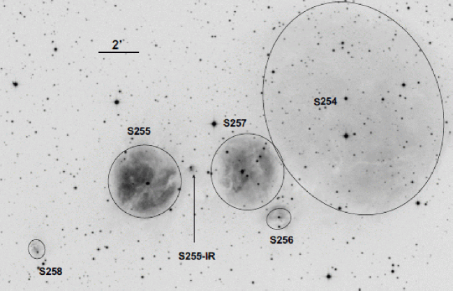
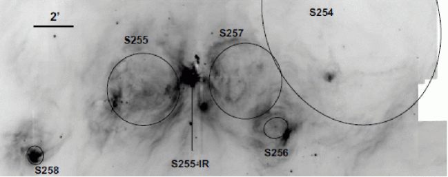
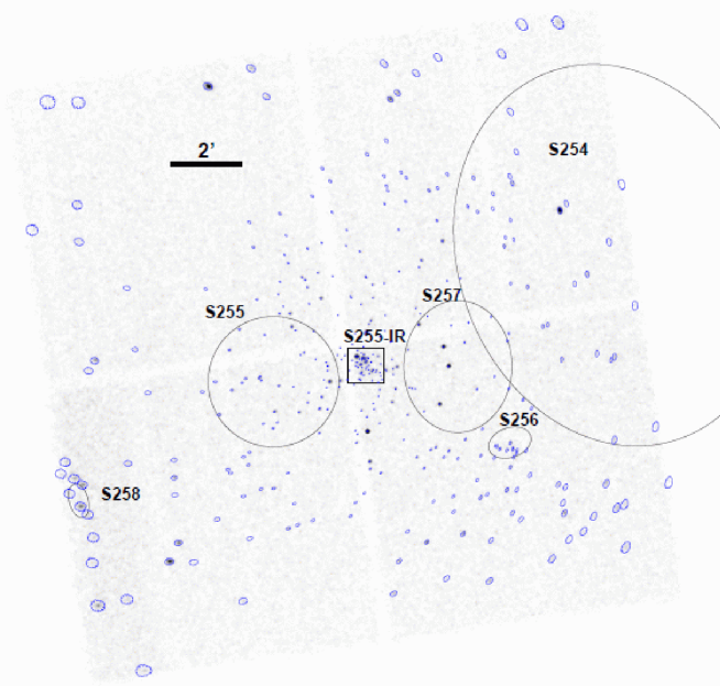
Figure 1: Top: Negative grayscale representation of the optical image of the S254-S258 complex from the Digitized Sky Survey. The black ellipses represent the five H II regions that define the complex. The location of the central, optically invisible embedded cluster S255-IR is marked by the arrow.
Center: Spitzer IRAC 4 image of the central part of the S254-S258 complex. This image was created from the basic calibrated data products for the programs 201 and 30784 retrieved from the Spitzer archive and mosaicked with the MOPEX software available from the Spitzer Science Center. Note that parts of the bright emission from the central embedded cluster S255-IR is saturated in these data.
Bottom: Chandra ACIS-I image of S254-S258 in the [0.5–8.0] keV band. Blue ellipsoids represent extraction regions for the individual detected X-ray sources based on a model of the local PSF that encircles 90% of total energy.

2.1 Chandra X-ray observations of S254-S258

The S254-S258 complex was observed (PI: Th. Preibisch) in November 2009 with the Imaging Array of the Chandra Advanced CCD Imaging Spectrometer (ACIS-I). ACIS-I provides a field of view of $17^{\prime}\times 17^{\prime}$ on the sky. At the 1.6 kpc distance of S254-S258 this corresponds to $7.9\times 7.9$ pc. The aimpoint of the observation was $\alpha({\rm J2000})=06^{\rm h}\,12^{\rm m}\,54.0^{\rm s}$, $\delta=+17\degr\,59^{\prime}\,24^{\prime\prime}$. The observation was performed in the standard “Timed Event, Faint” mode (with $3\times 3$ pixel event islands). The total net exposure time of 74 725 s (20.76 hours) was split into two parts, separated by about 4 days. The details of these two observation parts are given in Table 1. Since the roll angles (i.e. the orientation of the detector on the sky) is equal for both observations, each source is at the same detector position in both parts, making merging of these two data sets rather straightforward. Two of the CCDs of the ACIS-S spectroscopic array were also turned on during our observations. However, since the PSF at the large off-axis angles at these detectors is strongly degraded, their point-source sensitivity is reduced; only six X-ray sources are detected in the field of these ACIS-S chips.

The basic data products of our observation are the two Level 2 processed event list provided by the pipeline processing at the Chandra X-ray Center, that list the arrival time, location on the detector and energy for each of the 626 140 detected X-ray photons. We combined the two pointings with the merge_all script, a Chandra contributed software that make use of standard CIAO tools. The mean background count rate in our merged image, determined from several large source-free regions, is $2.95\times 10^{-7}$ counts s^-1 pixel^-1, corresponding to a mean background level of 0.02 counts pixel^-1.

Table 1: Chandra observation log

Obs.Id.	Date	Start – End Time [UT]	Exposure time	Level 2 events
10983	2009-11-16	11:40:48 – 23:35:08	40 570 s	340 411
12022	2009-11-20	05:14:15 – 15:18:20	34 155 s	285 729

At a distance of 1.6 kpc, the expected ACIS point source sensitivity limit for a 5-count detection on-axis in a 75 ks observation is $L_{\rm X,min}\sim 10^{29.5}$ erg s^-1, assuming an extinction of $A_{V}\leq 2.5$ mag ($N_{\rm H}\leq 5\times 10^{21}\,{\rm cm}^{-2}$) as typical for the stars in the H II regions, and a thermal plasma with $kT=1$ keV (which is a typical value for young stars; see, e.g., Preibisch et al., 2005). Using the empirical relation between X-ray luminosity and stellar mass and the temporal evolution of X-ray luminosity from the sample of young stars in the Orion Nebula Cluster that was very well studied in the Chandra Orion Ultradeep Project (Preibisch et al., 2005; Preibisch & Feigelson, 2005), we can expect to detect almost all stars in S254-S258 with masses greater than $0.5\,M_{\odot}$ and about half of the $0.1-0.5\,M_{\odot}$ stars. The expected level of detection completeness is $\ga 90\%$ for stars with $M_{\ast}\geq 0.5\,M_{\odot}$ (corresponding approximately to spectral types earlier than M1) and drops below 50% at $M_{\ast}\leq 0.25\,M_{\odot}$ (spectral types $\la$ M5). Note that these values are valid for the central part of the observed field; sensitivity is $\sim 3-4$ times worse at the edges of the ACIS field.

2.2 Source detection and X-ray source catalog

The source detection was performed in a two-step process. The first detection step was performed in a rather aggressive manner in order to find even the weakest possible sources, deliberately accepting some degree of false detections. In the second step, this list of potential sources was then cleaned from spurious detections by a detailed individual analysis. We employed the wavdetect algorithm (Freeman et al., 2002, a CIAO mexican-hat wavelet source detection tool) for locating X-ray sources in our merged image, and used a rather low detection threshold of 10^-5. This step was performed in three different energy bands, the total band [0.5-8.0] keV, the soft band [0.5-2.0] keV, and the hard band [2.0-8.0] keV, and with wavelet scales between 1 and 16 pixels. We also performed a visual inspection of the images and added some 30 additional candidates to the merged catalog from the wavelet analysis, resulting in a final catalog of 511 potential X-ray sources.

To clean this catalog from spurious sources, we then performed a detailed analysis of each individual candidate source with the ACIS Extract (AE hereafter) software package (Broos et al., 2010). A full description of the procedures used in AE can be found in Getman et al. (2005b), Townsley et al. (2003) and Broos et al. (2007). The following three steps were performed by AE in order to prune our input catalog from spurious detection (including afterglows):

1. Extraction regions were defined as the 90% contours of the local PSF (or smaller in the case of other nearby sources), and source events were extracted. Energy dependent corrections for the finite extraction regions were applied;

2. Local background events were extracted after masking all the sources in the catalog;

3. The Poisson probability ($P_{B}$) associated with the “null hypothesis”, i.e. that no source exist and the extracted events are solely due to Poisson fluctuations in the local background, is computed for each source.

All candidate sources with $P_{B}>0.01$ were rejected as background fluctuations. After 8 iterations of this pruning procedure our final catalog consisted of 364 sources. It contains 344 primary sources with $P_{B}<0.003$, and 20 tentative sources with $0.003<P_{B}<0.01$. The extraction regions for the sources in our final catalog are plotted on the Chandra image in Fig. 1.

2.3 X-ray point-source analysis with ACIS Extract

The AE software also determines basic properties for each of the detected sources, such as the net (i.e., background-subtracted) counts in various energy bands, the median photon energy, statistical test for variability, and a measure of the incident photon flux. These properties are reported in Table 2 2 (available in the electronic edition). Sources are sorted by increasing right ascension and identified by their sequence number (Col. 1) or their IAU designation (Col. 2). While the general X-ray properties were determined from the merged data set (the AE software is well suited for this purpose), we note that the spectra (see Sect. 3.1.3) were extracted from the individual observations.

2.4 Expected contamination of the X-ray source sample

As in any X-ray observation, there must be some degree of contamination by galactic field stars as well as extragalactic sources. To quantify the expected level of this contamination, we consider the results from the recent Chandra Carina Complex Project (CCCP; see Townsley et al., 2011), for which the individual pointings had very similar exposure times ($\approx 60-80$ ks) as our S254-S258 pointing. Furthermore, S254-S258 is at nearly the same galactic latitude as the Carina Nebula, suggesting that the background contamination should be very similar in these two regions.

For the CCCP data set, the classification study of Broos et al. (2011a), which considered the X-ray, optical, and infrared properties of the sources (that differ for the different contaminant classes), found that 716 X-ray sources in the 1.46 square-degree CCCP survey are are foreground stars, 16 are background stars, and 877 are extragalactic (AGN) contaminants. Scaling these numbers to the field-of-view of our S255 pointing gives 39 foreground stars, 1 background star, and 48 extragalactic (AGN) contaminants. However, since S254-S258 is considerably closer (1.6 kpc) than the Carina Nebula (2.3 kpc), the number of foreground stars should be accordingly smaller, approximately by a factor of $(1.6/2.3)^{3}\approx 0.34$. Furthermore, the number of foreground stars in the Carina Nebula is particularly high since this direction is close to the tangent point of the Carina spiral arm. These considerations imply that the contamination in our S254-S258 field should be clearly dominated by $\sim 48$ expected extragalactic sources (AGNs).

A characteristic of extragalactic contaminants is that their optical and infrared counterparts should be very faint, in fact mostly undetected in the available optical and infrared images. As we describe in more detail below, our search for counterparts of the X-ray sources left 46 X-ray sources outside the central embedded cluster S255-IR without optical or infrared counterparts. This number agrees well with the expected number of extragalactic contaminants.

Assuming at most 10 contaminating foreground/background stars, the total expected number of contaminants would be $\la 58$. With a total number of 364 detected X-ray sources, the expected level of contamination for our sample is thus $\la 15\%$.

3 Properties of the X-ray source in S254-S258

3.1 X-ray fluxes and luminosities

An accurate determination of the intrinsic X-ray source luminosities requires good knowledge of the X-ray spectrum. However, for the majority of the X-ray sources the number of detected photons is too low for a detailed spectral analysis. Only 25 sources in our catalog have more than 80 net counts, the practical lower limit for meaningful spectral analysis. For these bright sources we performed a detailed spectral fitting analysis to derive the plasma temperature and the extinction, and from these quantities we can calculate the intrinsic (i.e. , extinction-corrected) X-ray luminosities, as described in detail in Section 3.1.3.

For the weaker X-ray sources, for which a meaningful spectral analysis is not feasible, one cannot determine intrinsic X-ray luminosities without knowledge of the extinction. This is a substantial problem because the young stars in the S254-S258 complex show a very wide range of extinctions. There are numerous optically visible stars with low obscuration (at most a few magnitudes of visual extinction), while other stars suffer from cloud extinction up to about $A_{V}\sim 20$ mag, and embedded YSOs show additional circumstellar extinctions up to $A_{V}\sim 50$ mag and beyond (Chavarría et al., 2008). This implies that we cannot simply use a common count-rate to flux conversion factor to determine intrinsic X-ray luminosities but have to consider each source individually.

3.1.1 Observed X-ray fluxes

An estimate of the observed (i.e. not the intrinsic) X-ray flux is computed by AE. This quantity, called $FLUX2$, is calculated from the number of detected photons and using a mean value of the instrumental effective area (through the Ancillary Response Function, ARF) over energy. The $FLUX2$ values (derived for the full band, i.e. $[0.5-8]$ keV range), are reported in column (3) in Table 3 (available in the electronic edition). 3 It should be noted that this $FLUX2$ values suffer from a systematic error with respect to the true incident flux, because the use of a mean ARF is only correct in the hypothetical case of a flat incident spectrum, an assumption that probably not fulfilled. Nevertheless, the $FLUX2$ represents the best flux estimate that can be obtained for weak sources.

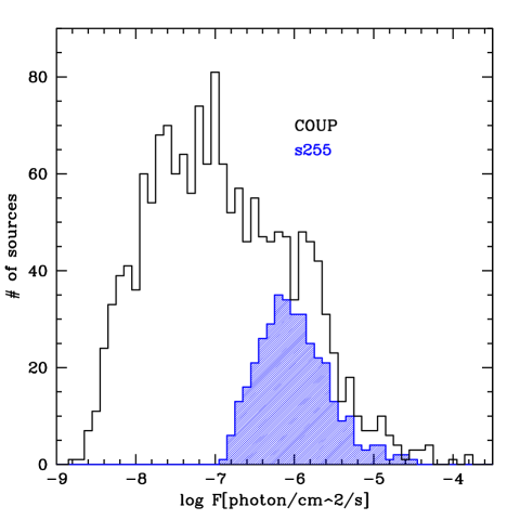
Figure 2: The blue histogram shows the distribution of FLUX2 values for the X-ray sources in S254-S258. For comparison, the distribution of fluxes from the COUP data from Getman et al. (2005b) is shown by the black histogram, scaled to the distance of S254-S258, i.e. 1.6 kpc.

In Figure 2 we compare the distribution of $FLUX2$ values for the S254-S258 sample to that of the stars in the Orion Nebula Cluster obtained in the context of the Chandra Orion Ultradeep Project (COUP, see Getman et al., 2005b). Note that the COUP fluxes were scaled to the 1.6 kpc distance of S254-S258. The two distribution show a very similar shape in the range between $\approx 10^{-6.0}$ photons cm^-2 s^-1 and $\approx 10^{-4.5}$ photons cm^-2 s^-1. The differences between the two distributions can be explained as follows:

First, the COUP sample shows a few stars with fluxes of $>10^{-4.5}$ photons cm^-2 s^-1, while no such very bright sources are seen in S254-S258. These very bright sources are the highly X-ray luminous O-type stars in the Orion Nebula Cluster. The fact that the S254-S258 does not contain such high-mass stars explains the absence of similarly high values in the observed distribution of incident fluxes for S254-S258.

Second, the peak and turn-over of the S254-S258 distribution at $\approx 10^{-6.2}$ photons cm^-2 s^-1 is a direct consequence of the higher sensitivity limit of our S254-S258 X-ray observation. As S254-S258 is about 4 times more distant than the ONC, and since the exposure time of our S254-S258 Chandra observation is less than one tenth of the 840 ks COUP observation, the expected sensitivity limit should be about 150 times higher.

Third, the number of sources per bin is always lower for S254-S258 compared to the ONC. This suggests that the total stellar population in the observed part of S254-S258 is smaller than in the ONC as observed in the COUP.

3.1.2 X-ray luminosities from XPHOT

An estimate of the intrinsic, i.e. extinction corrected, X-ray luminosity for sources that are too weak for a detailed spectral analysis can be obtained with the XPHOT software, developed by Getman et al. (2010). XPHOT is based on a non-parametric method for the calculation of fluxes and absorbing X-ray column densities of weak X-ray sources. X-ray extinction and intrinsic flux are estimated from the comparison of the apparent median energy of the source photons and apparent source flux with those of high signal-to-noise spectra that were simulated using spectral models characteristic of much brighter sources of similar class previously studied in detail. This method requires at least 4 net counts per source (in order to determine a meaningful value for the median energy) and can thus be applied to 255 of our 364 sources. Columns (4) to (7) of Table 2 report apparent and intrinsic (corrected for absorption, noted with subscript ${c}$) luminosities in the hard and total band, assuming a distance of 1.6 kpc. The resulting intrinsic X-ray luminosities range from $10^{29.4}$ to $10^{32.3}$ erg s^-1.

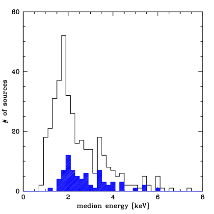
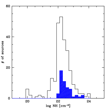
Figure 3: Distributions of median photon energies (left) and hydrogen column densities (right) determined by XPHOT (right) for the whole sample (black histograms). The blue dashed histograms show the distributions restricted to the sub-sample of sources located in the 1 arcmin radius region centered on the embedded cluster S255-IR.

Figure 3 shows the distribution of median photon energies and the deduced hydrogen column densities estimated by XPHOT. The median value of the derived hydrogen colum densities is $\log\left(N_{H}\,[{\rm cm^{-2}}]\right)=22.04$, corresponding to a visual absorption of $A_{V}\sim 6$ magnitudes. If we consider the sub-sample of sources located in the central embedded cluster S255-IR, this value rises to $\log\left(N_{H}\,[{\rm cm^{-2}}]\right)=22.21$ ($A_{V}\sim 9$ magnitudes), clearly showing stronger obscuration for the embedded sources.

3.1.3 X-ray spectral fits of bright sources

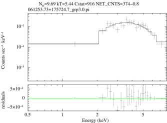
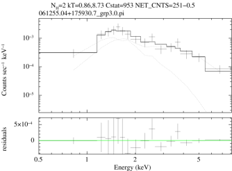
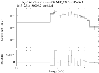
Figure 4: Chandra X-ray spectra and best-fit models of four bright X-ray sources in S254-258. The crosses show the measured spectra, the solid lines show the best-fit models; in the two cases where a two temperature model was required, the dotted lines show the two individual spectral model components. CXOU J061244.17+175914.0 is the B0.5 star HD 253327 that illuminates the S257 nebula. CXOU J061253.73+175724.7 is the source with the highest derived X-ray luminosity in our sample; it is located in the embedded cluster S255-IR. CXOU 061255.04+175930.7 is another embedded infrared source in S255-IR. CXOU 061312.58+180706.2 is the source with the second highest X-ray luminosity in our sample.

For the 25 sources in our sample with more than 80 net counts we performed a spectral fitting analysis using AE and the XSPEC software v12.5 (Arnaud, 1996). We used models with one- or two-temperature thermal VAPEC components (Smith et al., 2001) and the TBABS multiplicative model to describe the effect of extinction by interstellar (and circumstellar) material (as measured by the hydrogen column density $N_{H}$). The plasma abundances for the VAPEC components were fixed at the values adopted by the XEST study (Güdel et al., 2007) to be typical for pre-main sequence stars. For the extinction we used the standard interstellar abundances in the TBABS model as listed in Wilms et al. (2000). In order to evaluate the goodness of our fits we choose to apply the C-statistic (a maximum likelihood method; Cash (1979); Wachter et al. (1979)) which is better suited than the classic $\chi^{2}$ statistic for low-count data.

For two sources, # 97 and # 230, a two-temperature model was required for an acceptable fit. The remaining spectra are well fit with a single thermal component. A few selected examples of the spectral fits are shown in Figure 4. The spectral parameters are reported in Table 2. The hydrogen column densities range from $\log\left(N_{H}\,[{\rm cm^{-2}}]\right)=20$ to $\log\left(N_{H}\,[{\rm cm^{-2}}]\right)=23.08$, corresponding to visual absorptions between $A_{V}\la 0.1$ mag and $A_{V}\sim 65$ mag. These values are in good agreement with the estimates derived with XPHOT. The median value is 22.04, corresponding to $A_{V}\sim 6$ mag. The plasma temperatures range from $\approx 0.5$ keV (6 MK) up to $\sim 15$ keV (170 MK). In Table 2 we also report luminosities derived from the spectral fit, assuming a distance of 1.6 kpc. The intrinsic luminosities are calculated from the spectral fit parameters, setting extinction to zero. The range of extinction-corrected intrinsic X-ray luminosities spans from $\log L_{t,c}=30.56$ erg s^-1 to 32.11 erg s^-1 for the full [0.5-8.0] keV band.

The X-ray properties can give us some clues about the nature of the sources. The majority of the X-ray sources has plasma temperatures and X-ray luminosities in the typical ranges found for YSOs in other star forming regions (see, e.g., Preibisch et al., 2005); together with the fact that most X-ray sources have clear optical/infrared counterparts, this suggests that these X-ray sources actually are young stars in the S254-S258 complex. However, the sources for which the spectral fit yields extremely high plasma temperatures of $kT>7.5$ keV deserve special attention. Such very hard spectra are typical for extragalactic objects (AGNs), but also sometimes found for very young stellar objects (protostars) (see, e.g., Imanishi et al., 2001). As protostars are usually deeply embedded in the clouds in which they formed, the location of these very hard X-ray sources provides another hint towards their likely nature.

Considering these issues, source number 2 may well be an extragalactic contaminant. First, the spectral fit yields an extremely high temperature, but only moderate extinction. Second, this source has no optical/infrared counterpart, and, third, it is located at the periphery of the S254-S258 region, well outside the boundaries of the molecular clouds. Furthermore, its X-ray spectrum can also be well reproduced with a power-law model, as typical for AGN X-ray sources. Similar arguments apply to source 30.

The other X-ray sources with extremely high plasma temperatures are located in dense clouds, have infrared counterparts, and are thus probably deeply embedded very young stellar objects.

It is interesting to compare the X-ray luminosities from the spectral fits to those derived with XPHOT. Figure 5 shows that the results from these two different methods agree quite well for the majority of cases. Only for four of the highest luminosity objects we find that XPHOT seems to systematically over-estimate the X-ray luminosities by $\approx 0.1-0.2$ dex. The generally good agreement suggests that the X-ray luminosities derived with XPHOT are reliable. We therefore will use the XPHOT results for our analysis of the X-ray luminosity function presented below.

Table 2: Spectral parameters of brighter sources: the spectral fit was performed with an absorbed thermal plasma model with one (tbabs*vapec) or two components (tbabs*(vapec+vapec)).

Source	CP /	CXOU J	Net Counts	log $N_{H}$		$kT_{1}$		$kT_{2}$		log $L_{s}$	log $L_{h}$	log $L_{h,c}$	log $L_{t}$	log $L_{t,c}$
No.	IR class		(counts)	(cm-2)		(keV)		(keV)		(erg s-1)	(erg s-1)	(erg s-1)	(erg s-1)	(erg s-1)
(1)	(2)	(3)	(4)	(5)		(6)		(7)		(8)	(9)	(10)	(11)	(12)
1	yes	061147.81+180312.6	443.3	21.81$\pm$	0.15	0.7$\pm$	0.1	–		30.89	30.14	30.19	30.97	31.47
2	no	061154.83+180016.5	192.1	22.04$\pm$	0.46	15.0$\pm$	5.1	–		30.26	31.08	31.11	31.14	31.27
3	yes	061159.55+175802.9	159.6	22.38$\pm$	0.64	2.6$\pm$	1.2	–		30.21	30.96	31.05	31.03	31.40
5	yes / III	061206.65+180336.6	239.0	21.41$\pm$	0.16	0.5$\pm$	0.1	–		30.88	29.55	29.57	30.90	31.17
27	yes	061230.43+175506.8	81.8	20.48$\pm$	0.19	9.4$\pm$	9.9	–		30.23	30.53	30.53	30.70	30.71
30	yes	061230.98+180336.9	386.2	22.07$\pm$	0.13	15.0∗		–		30.62	31.46	31.49	31.52	31.65
32	yes	061231.17+180853.8 F	99.5	21.96$\pm$	0.41	3.8$\pm$	2.3	–		30.28	30.78	30.81	30.90	31.09
97	yes / III	061244.17+175914.0	174.6	21.56$\pm$	0.26	0.6$\pm$	0.2	3.4$\pm$	1.6	30.57	30.45	30.46	30.81	31.02
102	yes	061244.76+175946.8	156.6	21.61$\pm$	0.15	3.1$\pm$	0.8	–		30.41	30.65	30.67	30.85	30.98
104	yes	061245.23+175810.3 F	116.6	20.0∗		1.5$\pm$	0.2	–		30.45	30.06	30.06	30.60	30.61
113	yes / III	061246.71+175418.2	86.6	21.53$\pm$	0.23	0.7$\pm$	0.1	–		30.38	29.47	29.49	30.43	30.73
147	yes / III	061251.04+180644.1	141.8	20.00$\pm$	16.03	1.0$\pm$	0.1	–		30.69	29.66	29.66	30.73	30.74
183	yes	061253.48+175633.9	91.2	23.08$\pm$	3.43	54.2$\pm$	724	–		28.43	31.13	31.35	31.13	31.48
190	yes	061253.73+175724.7	373.2	22.99$\pm$	1.25	5.4$\pm$	1.2	–		29.51	31.64	31.88	31.65	32.11
209	yes	061254.33+175927.7 F	86.5	22.86$\pm$	1.99	8.6$\pm$	10.8	–		29.13	30.99	31.16	31.00	31.35
230	yes	061255.04+175930.7 F	250.5	22.30$\pm$	0.53	0.9$\pm$	0.4	8.7$\pm$	13.0	30.44	31.11	31.18	31.20	31.61
255	yes / I	061258.21+175848.1	91.7	22.34$\pm$	0.53	2.6$\pm$	0.9	–		30.00	30.70	30.79	30.78	31.14
333	yes	061312.58+180706.2	379.7	22.56$\pm$	0.46	7.9$\pm$	3.5	–		30.33	31.60	31.70	31.63	31.90
337	no	061316.04+175416.7	139.9	22.22$\pm$	0.42	3.9$\pm$	1.6	–		30.19	30.91	30.96	30.98	31.24
341	yes	061317.11+175344.9 F	265.6	21.74$\pm$	0.17	5.0$\pm$	1.6	–		30.70	31.16	31.17	31.29	31.41
348	yes / II	061325.57+175230.5	163.1	22.18$\pm$	0.39	1.6$\pm$	0.3	–		30.44	30.73	30.81	30.91	31.35
349	yes / III	061325.94+175923.5 F	95.6	20.0∗		1.0$\pm$	0.3	–		30.48	29.73	29.73	30.55	30.56
354	yes	061327.41+175554.3	125.2	21.91$\pm$	0.3	5.6$\pm$	4.1	–		30.25	30.82	30.85	30.93	31.08
355	yes	061327.61+175517.8	182.8	22.11$\pm$	0.35	3.8$\pm$	1.4	–		30.38	31.00	31.05	31.10	31.32
359	yes	061328.37+175604.4	97.7	22.15$\pm$	0.52	4.3$\pm$	2.6	–		30.07	30.75	30.80	30.84	31.06
∗ indicates frozen parameters in the fit.
Col. (2): presence of an optical or infrared counterpart, infrared class from Spitzer photometry (if available).
Col. (3): sources flagged with “F” showed flare-like variability during our observations; lightcurves are shown in Fig. 6.
Col. (4): absorbing hydrogen column density of the best-fit.
Cols. (5) and (6): plasma temperature(s) of the best-fit.
Cols. (7) to (11): X-ray luminosities (for an assumed distance of 1.6 kpc) in the soft (${s}$, [$0.5-2.0$] keV) band, the hard (${h}$ [$2.0-8.0$] keV) band, and the total (${t}$ [$0.5-8.0$] keV) band.
Absorption-corrected luminosities are denoted with the subscript ${c}$.

Figure 5: Comparison of the intrinsic full band [0.5-8.0] keV luminosities derived from the spectral fits to the 25 bright sources (Table 2) to the intrinsic full band [0.5-8.0] keV luminosities determined with XPHOT.

3.2 X-ray source variability

Figure 6: Lightcurves for six significantly variable sources. The solid dots show the arrival time (measured from the start of the observation) and the energy of each of the detected source photons. The histograms show the corresponding binned lightcurves.

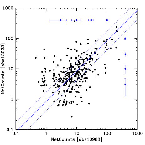
Figure 7: This plot shows for each X-ray source the net counts in the first pointing compared to the net counts in the second pointing (obtained about 4 days later). The sequence of blue error bars at the upper and right edge show the Poisson statistical uncertainties for different numbers of net counts. The solid line indicates the expected relation for sources with constant count rates in the two pointings; the dotted lines are offset by factors of 2.

A first analysis of the time variability of individual X-ray sources is performed by AE by comparing the arrival times of the individual source photons in each extraction region to a model assuming temporal uniform count rates. The statistical significance for variability is quantified computing the 1-sided Kolmogorov-Smirnov statistic (Col. 15 of Table 2). In our sample, 23 sources show significant X-ray variability (probability of being constant $P_{\rm const}<0.005$) and 19 are classified as possibly variable ($0.005<P_{\rm const}<0.05$).

The light curves of the variable X-ray sources show a variety of temporal behavior; six of the most interesting lightcurves are shown in Fig. 6. Five of these sources show flare-like variability, i.e. a fast increase of the count rate followed by a slow exponential decay, as typical for solar-like magnetic reconnection flares (see, e.g., Favata et al., 2005; Wolk et al., 2005; Preibisch et al., 1993). The other variable sources show irregular variability or slowly increasing or decreasing countrates. This kind of X-ray variability is typical for young stellar objects (see, e.g., Stassun et al., 2006).

We also investigated time variability by comparing the count rate for each source of the two single Chandra pointings, i.e. at a time difference of about 4 days (see Figure 7). One can see that the majority of sources show changes in the count rates by less than a factor of 2. Only for 21 sources the count rates differ by more than 3$\sigma$ between the two observations. The result is consistent with the assumption that the X-ray emission from young stellar objects is a superposition of many flares of different amplitude, where weak flares are very frequent while very strong flares occur more rarely, at rates of about one such event per week (e.g., Getman et al., 2008).

4 Characteristics of the X-ray stellar population of S254-S258

4.1 Optical and infrared counterparts of the X-ray sources

In order to identify counterparts of the X-ray sources in other wavelengths, we used the optical images from the Digitized Sky Survey (DSS), the Two Micron All Sky Survey (2MASS) point source catalog, and the Spitzer-IRAC catalog from Chavarría et al. (2008). The results of the cross-correlation are reported in Table 5 (available in the electronic edition). 5 Our visual inspection of the red and blue DSS images gave optical counterparts to 95 X-ray sources (i.e. 26% of all 364 X-ray sources). Our cross-correlation with the 2MASS Point Source Catalog lead to 231 near-infrared counterparts (i.e. a counterpart fraction of 63%). Our cross-correlation with the infrared catalog from Chavarría et al. (2008) yielded 293 infrared counterparts, i.e. 80% counterpart fraction. For 58 X-ray sources we did not find a counterpart in any of the inspected optical and infrared images. Twelve of these sources are located in or very close to the central embedded cluster S255-IR. These X-ray sources may be very deeply embedded protostars or young stellar objects located behind the dense molecular cloud clumps; the non-detection of optical/infrared counterparts would then be related to very high extinction. The remaining 46 X-ray sources without known optical/infrared counterpart outside this cluster show a rather homogeneous spatial distribution, as expected for (mostly extragalactic) contaminants.

It is interesting to consider the infrared classification of these sources based on the IRAC spectral energy distribution (SED) slope determined by Chavarría et al. (2008). Unfortunately, the matching of our X-ray source-list with this infrared catalog is not straightforward. The catalog contains 26 821 infrared sources. However, most of these are only detected in the deep near-infrared images, and just about 6400 of these are detected in the Spitzer data. Infrared classifications are only available for the 462 infrared sources that are detected in all four IRAC bands. The majority of the catalog entries are very faint NIR sources, and many of these are probably background objects rather than young stars in S254-S258. Furthermore, the fact that only 4225 of the 26 821 sources are detected in all three of the $J$-, $H$-, and $K$-bands also suggest that there may well be a significant number of spurious detections among the faint sources detected in only one band. This very high number of faint infrared sources produces serious problems in any attempt to find the correct infrared counterparts for our X-ray sources, since many Chandra sources have more than one possible counterparts within the X-ray error radius. In these cases, the closest positional match is not necessarily the true counterpart. Due to the increasing number of infrared sources at fainter magnitudes, good positional matches with very faint infrared sources may in fact be just chance superpositions of physically unrelated sources, and one of the other possible matches may be the true counterpart. A reliable identification of the infrared counterparts requires a sophisticated approach and will be addressed in the next step of our study. Nevertheless, we can mention here the results of a preliminary source matching, where we only considered the spatially closest match to each X-ray source. We find that 8 X-ray sources have closest matches classified as Class I YSOs (embedded very young stellar objects with infalling envelopes), 50 X-ray sources have closest matches classified as Class II YSOs (Classical T-Tauri stars, CTTs), and 8 X-ray sources have closest matches classified as Class III YSOs (“Weak line” T-Tauri stars, WTTs) in the infrared catalog.

4.2 The X-ray luminosity function

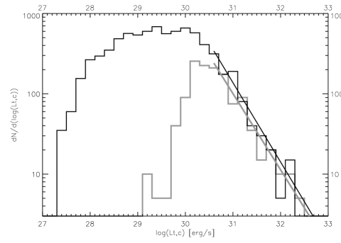
Figure 8: Comparison of the XLF of S254-S258 (thick grey line) to the XLF of the Orion Nebula Cluster (from the COUP data; Getman et al., 2005b, black line). The straight lines show the results of the power-law fits to the distributions in the luminosity range $L_{\rm X}=10^{30.5}\,-\,10^{32.0}$ erg s^-1.

The X-ray luminosity function (XLF) is the product of the distribution of X-ray luminosities of stars with a given mass and the number of stars per mass interval, i.e. the initial mass function (IMF). Although the correlation between stellar mass and X-ray luminosity shows a considerable scatter (see, e.g., Preibisch et al., 2005), X-ray studies of a large number of young stellar clusters have shown that the XLF appears to be rather universal and constant in different environments (see Feigelson & Getman, 2005; Getman et al., 2006; Wang et al., 2007).

To construct the XLF of S254-S258, we use the intrinsic full band [$0.5-8.0$] keV luminosities calculated by XPHOT (Table 3 column (7)). Our XLF of S254-S258 is shown in Figure 8 and compared to the XLF for the stars in the Orion Nebula Cluster from the COUP (Getman et al., 2005b). Obviously, the S254-S258 XLF peaks and turns over at a higher luminosity (near $L_{\rm X}\approx 10^{30.3}$ erg s^-1) than the COUP XLF, because the X-ray detected sample for S254-S258 is incomplete for low-mass stars due to the lower sensitivity as discussed above. The slopes of the bright parts of these two distributions, however, can be seen to agree well.

For a more quantitative analysis, we performed power-law fits of the form $dN/d(\log L_{\rm X})\propto\alpha\times\log L_{\rm X}$ for the observed distribution of luminosities. We used the maximum-likelihood technique described by Maschberger & Kroupa (2009), that yields an estimate for the exponent from the observed distribution function (i.e. not a fit of the histogram). The resulting power-law exponents for the distribution of X-ray luminosities in the range $L_{\rm X}=[10^{30.5}-10^{32.0}]$ erg/s are $\alpha=-0.95\pm 0.09$ for the Orion COUP data, and $\alpha=-0.91\pm 0.10$ for our S254-S258 data. This consistency confirms the results from comparisons of other regions (e.g., the CCCP; Feigelson et al., 2011).

This result shows that it is reasonable to assume that the XLF of S254-S258 has a similar shape as the ONC XLF. We can therefore make a quantitative estimate of the size of the total young stellar population in the observed part of S254-S258 by determining the vertical offset between the two distributions. We find that the total population in the observed part of the S254-S258 complex is $\approx 0.7\times$ of that in the ONC. Since the total population of the Orion Nebula Cluster (within 2.06 pc, Hillenbrand & Hartmann 1998) is about 2800 stars, the observed region of the S254-S258 should contain $\sim 2000$ stars in total.

4.3 Spatial distribution of the X-ray sources

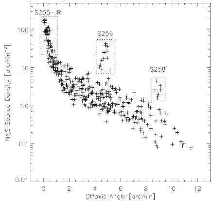
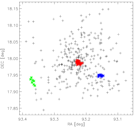
Figure 9: Top: Nearest neighbor analysis surface density at the location of each X-ray source plotted against the offaxis-angle. The general decrease of density with increasing offaxis-angle is related to instrumental effects. The dot-lined boxes mark the members of the three identified clusters.
Bottom: Spatial distribution of the X-ray sources. The members of the three clusters marked in the top plot are show by the colored asterisks.

The spatial distribution of the 364 X-ray sources in the Chandra field shows a complex pattern. Besides the prominent and dense central cluster S255-IR a few further apparent clusterings as well as a widely distributed population of X-ray sources that are spread homogeneously over the entire field-of-view of our Chandra observation can be seen. For a quantitative characterization of the spatial distribution we performed a nearest neighbor analysis (see Casertano & Hut, 1985) to identify statistically significant clusterings in an objective way. The surface density estimator at the position of each source $i$ is given by $\mu_{j}(i)=(j-1)\big{/}\left(\pi\,{D_{j}(i)}^{2}\right)\,,$ where $D_{j}(i)$ is the angular distance from source $i$ to its $j$th nearest neighbor. We used $j=5$ for our analysis; this value is large enough to keep the fluctuations of the local density estimates reasonably low and at the same time allows to detect groups with a minimum of $\sim 5$ stars. For the interpretation of the resulting densities, we have to take the spatial variations of the detection sensitivity over the field-of-view into account. The sensitivity is highest in the center, but due to effects such as mirror vignetting and the increasing width of the point-spread function, it gets several times worse near the edges of the ACIS field-of-view. We therefore plot in Fig. 9 the source density $\mu_{5}$ as a function of the offaxis-angle. The general trend of decreasing source density with increasing offaxis-angle can be clearly seen.

Clusters can be defined as spatially confined groups of sources for which the local surface density clearly exceeds the values found at other locations in the image at similar offaxis-angles. The obvious dense central cluster S255-IR appears (as expected) as a very prominent peak at low offaxis-angles in Fig. 9. Using a density threshold of $\mu_{5}\geq 22\,\rm arcmin^{-1}$, we find that 45 X-ray sources can be considered as members of this cluster. Two further prominent peaks can be seen in the plot: one peak consisting of 12 sources near offaxis-angle $5^{\prime}$ is caused by a cluster of sources in the S256 region, while another peak around offaxis-angle $9^{\prime}$ with 7 sources represents a clustering in the S258 region.

Our clustering analysis thus reveals three significant clusters, that contain a total population of 64 X-ray sources. The remaining 300 X-ray sources are thus in a distributed, non-clustered spatial configuration. As discussed above, up to $\approx 50$ X-ray sources may be unrelated contaminants. This leads to a population of $\sim 250$ widely distributed X-ray detected young stars in the observed area.

5 The size of the distributed X-ray population

In order to check whether the distributed X-ray sources may represent the low-mass stellar population associated to the B0 stars in S255 and S257, we compare the size of the distributed X-ray population with the expected number of based on IMF extrapolations. According to the Kroupa (2001) field IMF model, each B0 star ($M\approx 15\,M_{\odot}$; see Martins et al., 2005) should be associated by $\approx 320$ low-mass stars $([0.1-2]\,M_{\odot})$. However, not all of these low-mass stars will be detected in our X-ray observation, as the X-ray luminosities of young stars are related to the stellar mass. The expected number of X-ray sources can be found by comparing the X-ray detection limit to the typical X-ray luminosity functions for young stars in specific mass ranges.

As discussed above, the X-ray detection limit of our data is $L_{\rm X,min}\sim 10^{29.5}$ erg s^-1 in the central part of the observed field. However, this limit shows considerable systematic variations as a function of the off-axis angle and gets several times worse near the edges of the ACIS field. If we consider the widely distributed population of X-ray sources, we have to take into account that most of these sources are located outside the central few arcmininute region of maximum sensitivity. Broos et al. (2011b) performed a detailed analysis of the spatial sensitivity variations over the ACIS field. From the values for the completeness limits in different off-axis angle slices in their Table 8 we find that the area-weighted average of the completeness limit over the full field-of-view is about 0.5 dex higher than the on-axis value. This implies that the average X-ray completeness limit of our Chandra data for the widely distributed population is thus $\log L_{\rm X}\sim 10^{30.0}$ erg s^-1.

Since the X-ray luminosity functions for young stars are very similar for most studied regions (see Feigelson & Getman, 2005; Getman et al., 2006) we can assume that the young stars in S254-S258 follow the same relations between stellar mass and X-ray luminosity as established by the data from the Chandra Orion Ultradeep Project (see Preibisch & Feigelson, 2005). This implies that we should detect $\approx 70\%$ of the young stars in the mass range $[0.5-2]\,M_{\odot}$ and $\approx 30\%$ of the stars in the mass range $[0.1-0.5]\,M_{\odot}$.

Since the Kroupa (2001) IMF predicts $\approx 80$ stars with $[0.5-2]\,M_{\odot}$ and $\approx 250$ stars with $[0.1-0.5]\,M_{\odot}$ for each B0 star, the expected number of X-ray detected stars associated to the two B0 stars is $\sim 2\times(0.7\times 80+0.3\times 250)=262$. The observed number of $\approx 250$ distributed X-ray sources (after correction for background contamination) is actually quite close to this expectation value and consistent with the assumption that these X-ray sources trace the low-mass stellar population associated to the two B-stars.

6 Conclusions

Our deep Chandra observation of the S254-S258 complex led to the detection of 364 X-ray sources, about 50 of which are expected to be background contaminants. The X-ray properties of most sources (luminosity, plasma temperature, and variability) are in the typical ranges found for young stellar objects. This supports the assumption that these X-ray sources objects represent the population of young low-mass stars in the S254-S258 complex. Our analysis of the spatial distribution of the X-ray sources with a nearest neighbor method reveals three significant clusters: the dense central cluster S255-IR, and two smaller clusterings related to S256 and S258. About 20% of the X-ray sources are members of one of these clusters, whereas the large majority $(\sim 80\%$) of the X-ray sources traces a widely distributed population of young stars.

The size of this distributed population of X-ray detected young stars is in good agreement with the expected X-ray source number based on the assumption that these stars trace the low-mass population associated with the two early B-type stars in S255 and S257. We would not expect to see this distributed population in the context of the models that two B0 stars have either formed in isolation or were ejected from the central embedded cluster. Our results therefore suggest that the two B-stars and the associated distributed low-mass stars represent a stellar population that is distinct from the embedded cluster of YSOs in S255-IR. This is in agreement with the model scenario in which the observed star formation activity in the dense embedded cluster located in the interaction zone between the S255 and S257 H II regions has been triggered by the compression of the cloud due to the expansion of the H II regions.

A detailed analysis of the optical and infrared properties of the individual X-ray detected young stars that can provide direct information on the ages, masses, and the circumstellar disks around these stars will be presented in a upcoming study.