On the sdOB primary of the post common-envelope binary AA Doradus (LB 3459)††thanks: Based on observations made with ESO Telescopes at the Paranal Observatories under programme ID 66.D-1800.
Abstract
Context. AA Dor is an eclipsing, post common-envelope binary with an sdOB-type primary and a low-mass secondary. Eleven years ago, an NLTE spectral analysis showed a discrepancy in the surface gravity that was derived by radial-velocity and light-curve analysis, () and , respectively.
Aims. We aim to determine both the effective temperature and surface gravity of AA Dor precisely from high-resolution, high-S/N observations taken during the occultation of the secondary.
Methods. We calculated an extended grid of metal-line blanketed, state-of-the-art, non-LTE model atmospheres in the parameter range of the primary of AA Dor. Synthetic spectra calculated from this grid were compared to optical observations.
Results. We verify from our former analyses and determine a higher . The main reason are new Stark-broadening tables that were used for calculating of the theoretical Balmer-line profiles.
Conclusions. Our result for the surface gravity agrees with the value from light-curve analysis within the error limits, thereby solving the so-called gravity problem in AA Dor.
Key Words.:
Stars: abundances – Stars: atmospheres – Stars: binaries: eclipsing – Stars: early-type – Stars: low-mass – Stars: individual: AA Dor, LB 34591 Introduction
AA Dor is a close, eclipsing, post common-envelope binary system with an sdOB-type primary star and an unseen low-mass companion. The orbital period is 0.261 539 7363 (4) d (Kilkenny 2011) and the inclination is (Hilditch et al. 2003). A detailed introduction to the system and previous analyses is given in Rauch (2004), and we summarize results of previous spectral analyses of the primary in Table 1.
| He | ) | method | reference | ||||||||||
|---|---|---|---|---|---|---|---|---|---|---|---|---|---|
| (K) | (cm/sec2) | (mass fraction) | (km/sec) | () | () | ||||||||
| 41000 | 5. | 4 | 0. | 28 | LTE1 | Kudritzki (1976) | |||||||
| 44200 | 5. | 2 | 0. | 28 | NLTE1 | Kudritzki (1976) | |||||||
| 41700 | 5. | 9 | 0. | 8 | LTE1 | Kudritzki (1976) | |||||||
| 42000 | 5. | 7 | 0. | 8 | NLTE1 | Kudritzki (1976) | |||||||
| 40000 | 5. | 3 | 0. | 012 | 0. | 3 | 0. | 04 | NLTE1 | Kudritzki et al. (1982) | |||
| 42000 | 1000 | 5. | 21 | 0. | 0032 | 34. | 0 | 0. | 33 | 0. | 066 | NLTE2 | Rauch (2000) |
| 42000 | 1000 | 5. | 30 | 0. | 0032 | 35. | 0 | NLTE3 | Fleig et al. (2008) | ||||
| 37800 | 500 | 5. | 51 | 0. | 005 | 30. | 0 | 0. | 51 | 0. | 085 | LTE4 | Müller et al. (2010) |
| 42000 | 1000 | 5. | 46 | 0. | 0027 | 30. | 0 | 0. | 47 | 0. | 079 | NLTE5 | this work |
1 H+He models, two grids with fixed / ratios only, investigation of NLTE effects, no errors given
2 H+He+C+N+O+Mg+Si+Fe+Ni, Fe+Ni data from Kurucz (1991), optical spectra, assumed bound rotation ()
3 H+He+C+N+O+Mg+Si+P+S+Ca+Sc+Ti+V+Cr+Mn+Fe+Co+Ni, Ca-Ni data from Kurucz (1991), optical and FUV spectra
4 H+He metal enhanced ( = ten times solar), optical spectra
5 H+He+C+N+O+Mg+Si+P+S+Ca+Sc+Ti+V+Cr+Mn+Fe+Co+Ni, Ca-Ni data from Kurucz (2009), optical spectra, from Müller et al. (2010)
Rauch (2000) encountered the problem of his spectroscopically determined surface gravity not matching determined from light-curve analysis (Hilditch et al. 1996). Hilditch et al. (2003) present an improved photometric model and derive . The reason for the discrepancy is unknown. Fleig et al. (2008) find a slightly higher but the discrepancy remains. A recent analysis by Müller et al. (2010) has apparently solved the problem by finding .
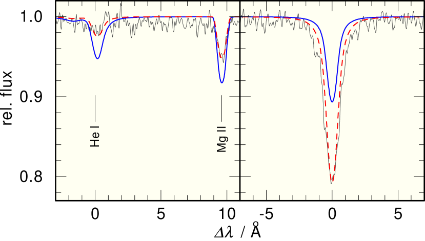
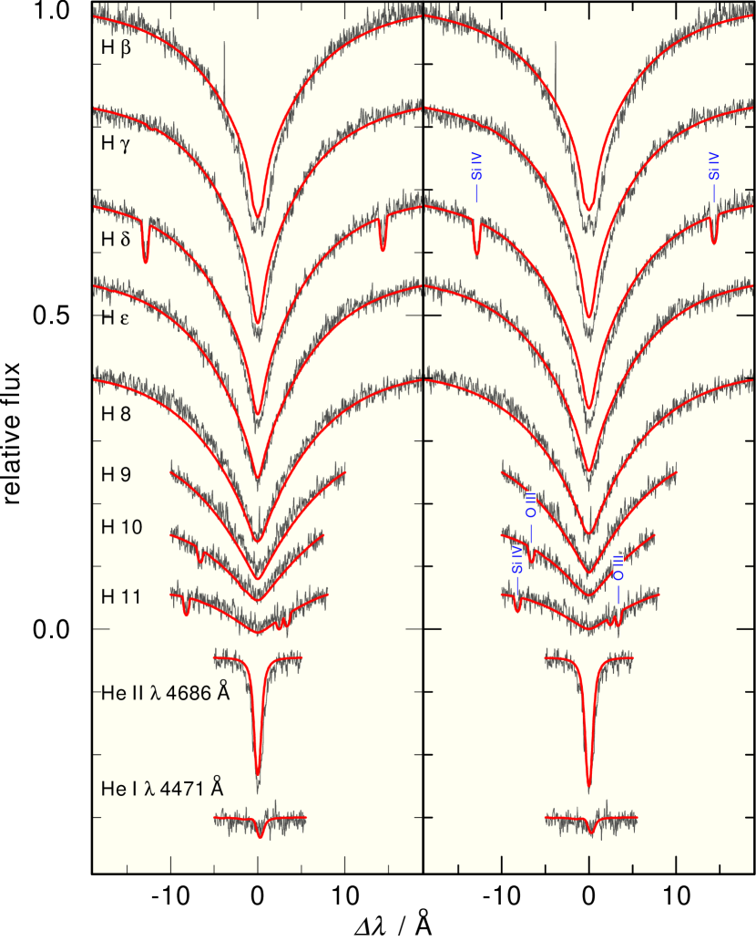
Müller et al. (2010) do not consider that the He I lines (as well as other lines of low-ionized species, e.g. of Mg II, Fig. 1) are too strong in the models at their favored parameters and , as demonstrated in Fig.1. Increasing the He abundance to better fit He II Å also results in a much stronger He I Å, which then disagrees with the observation. We mention that Fleig et al. (2008) evaluate the ionization equilibria of C III / C IV, N III / N IV, O III / O IV, P IV / P V, and S IV / S V in the FUV wavelength range and find to agree with the higher concluded from the He I lines.
Since Kurucz (2009, http://kurucz.harvard.edu/atoms.html) has substantially extended his database, and the model atoms in our Tübingen Model-Atom Database (TMAD111http://astro.uni-tuebingen.de/TMAD/TMAD.html) have been updated as well, we decided to calculate an improved, extended, state-of-the-art NLTE model-atmosphere grid. This grid is described in Sect. 2. The re-analysis of our UVES spectra (105 á 180 sec, which in total cover one orbital period and which were also used by Müller et al. 2010) that were obtained in 2001 at the VLT is described in Sect. 3. We conclude in Sect. 4.
2 Atomic data and model-atmosphere grid
The model atmospheres used here were calculated with the Tübingen Model-Atmosphere Package (Werner et al. 2003, TMAP). The models are plane-parallel, in hydrostatic and radiative equilibrium. TMAP uses the occupation-probability formalism of Hummer & Mihalas (1988) that was generalized to NLTE conditions by Hubeny et al. (1994). TMAP considers opacities of H+He+C+ N+O+Mg+Si+P+S using classical model atoms, and Ca+Sc+Ti+V+Cr+Mn+Fe+Co+Ni uses a statistical approach (Rauch & Deetjen 2003). All model atoms used in our calculations were updated to the most recent atomic data (Sect. 1), and 530 levels are treated in NLTE with 771 individual lines (from H - S) and 19 957 605 lines of Ca - Ni from Kurucz’ line lists (Kurucz 2009) combined to 636 superlines. The element abundances are summarized in Table 2.
2
| element | mass | number | ||||||
|---|---|---|---|---|---|---|---|---|
| X | fraction | fraction | []∗ | [X]∗∗ | ||||
| H | 9. | 939E1 | 9. | 992E1 | 12. | 144 | 0. | 130 |
| He | 2. | 686E3 | 6. | 801E4 | 8. | 977 | 1. | 967 |
| C | 1. | 777E5 | 1. | 499E6 | 6. | 320 | 2. | 124 |
| N | 4. | 145E5 | 2. | 998E6 | 6. | 621 | 1. | 223 |
| O | 1. | 009E3 | 6. | 393E5 | 7. | 950 | 0. | 754 |
| Mg | 4. | 078E4 | 1. | 700E5 | 7. | 375 | 0. | 240 |
| Si | 3. | 049E4 | 1. | 100E5 | 7. | 186 | 0. | 339 |
| P | 5. | 197E6 | 1. | 700E7 | 5. | 375 | 0. | 050 |
| S | 3. | 241E6 | 1. | 024E7 | 5. | 155 | 1. | 980 |
| Ca | 5. | 994E5 | 1. | 515E6 | 6. | 325 | 0. | 030 |
| Sc | 3. | 694E8 | 8. | 327E0 | 3. | 065 | 0. | 100 |
| Ti | 2. | 784E6 | 5. | 894E8 | 4. | 915 | 0. | 050 |
| V | 3. | 731E7 | 7. | 421E9 | 4. | 015 | 0. | 070 |
| Cr | 1. | 663E5 | 3. | 240E7 | 5. | 655 | 0. | 001 |
| Mn | 9. | 877E6 | 1. | 828E7 | 5. | 405 | 0. | 040 |
| Fe | 1. | 153E3 | 2. | 091E5 | 7. | 465 | 0. | 050 |
| Co | 3. | 591E6 | 6. | 174E8 | 4. | 935 | 0. | 069 |
| Ni | 3. | 482E4 | 6. | 009E6 | 6. | 923 | 0. | 689 |
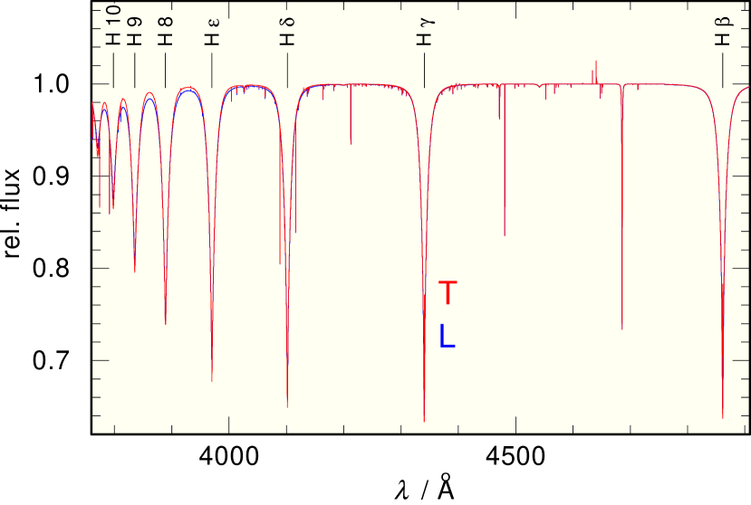
The model-atmosphere grid spans ( ) and ( ). In total this makes 638 models. Spectral energy distributions (SEDs) were calculated using the most recent line broadening data, e.g. H i line-broadening has changed in TMAP since Fleig et al. (2008) presented their analysis of AA Dor. The reason is that Repolust et al. (2005) found an error in the H i line-broadening tables (for high members of the spectral series only) by Lemke (1997) that were used before. These were substituted by a Holtsmark approximation. In addition, Tremblay & Bergeron (2009) provide new, parameter-free Stark line-broadening tables for H i considering non-ideal effects. These replaced Lemke’s data for the lowest ten members of the H i Lyman and Balmer series. In the parameter range of AA Dor, the new broadening tables have a significant impact on the line wings of higher Balmer-series members (narrower for H and higher, Fig. 2). As a consequence, our analysis results in a higher (Sect. 3).
In the framework of the Virtual Observatory222http://www.ivoa.net (VO), all these SEDs () are available in VO compliant form via the VO service TheoSSA333http://vo.ari.uni-heidelberg.de/ssatr-0.01/TrSpectra.jsp? provided by the German Astrophysical Virtual Observatory (GAVO444http://www.g-vo.org).
3 Analysis and results
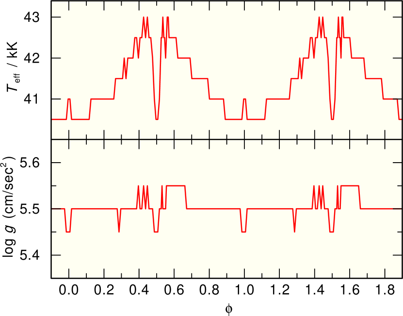
The light curve of AA Dor exhibits a reflection effect (e.g. Hilditch et al. 1996) that amounts to about 0.06 mag in the optical. To analyze the pure primary spectrum, we selected only those four observations that were taken closest to the occultation of the secondary. These were co-added in order to improve the S/N. In Fig. 3, we show a fit to all single UVES spectra. Our fit excludes the inner line cores of H and H , as well as obviously bad data points (quality flags given by Müller et al. 2010). Both the occultation (at ) and the transit () of the secondary are clearly visible in the determination of and . Compared to a similar fit of Müller et al. (2010, their Fig. 3), we find the same but a significantly higher than for .
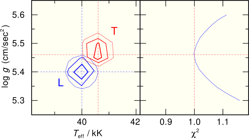
For the analysis, we perform a detailed comparison in the classical way (-by-eye) and, for comparison in analogy to Müller et al. (2010) with a fit, used the same wavelength limits (Table 3) and lines, H - H 11 and He II Å. Our fit yields and (T in Fig. 4). These errors are formal errors, and was calculated from the deviation of the model from the observed spectrum used in the fit. Compared to a similar fit with SEDs that were calculated with the previously used Stark broadening tables of Lemke (1997, L in Fig. 4), there is a significant deviation of and .
3
| line | line | ||||
|---|---|---|---|---|---|
| (Å) | (Å) | ||||
| H | [50, | +50] | He I Å | [ 5, | +5] |
| H | [40, | +40] | He II Å | [ 5, | +5] |
| H | [30, | +30] | |||
| H | [20, | +20] | |||
| H 8 | [20, | +20] | |||
| H 9 | [10, | +10] | |||
| H 10 | [10, | +7] | |||
| H 11 | [10, | +8] | |||
A comparison of the best-fitting model from our fit and the best-fitting -by-eye with the observations is shown in Fig. 5. It is obvious that the ionization equilibrium of He I / He II is reproduced not at but at . The theoretical line profiles of lower members of the Balmer series (H - H ) do not reproduce the observation perfectly. They fit slightly better at . Thus, a small Balmer-line problem (Napiwotzki & Rauch 1994; Werner 1996) due to additional metal opacities that are still not considered is apparently present. The inclusion of He I Å (Table 3) in the -fit procedure results in higher . We finally adopt (cf. Fleig et al. 2008) and because the previously evaluated ionization equilibria (Rauch 2000; Fleig et al. 2008) are an additional, crucial constraint. A fit at fixed (additional models were calculated with and ) also has its minimum at (Fig. 4).
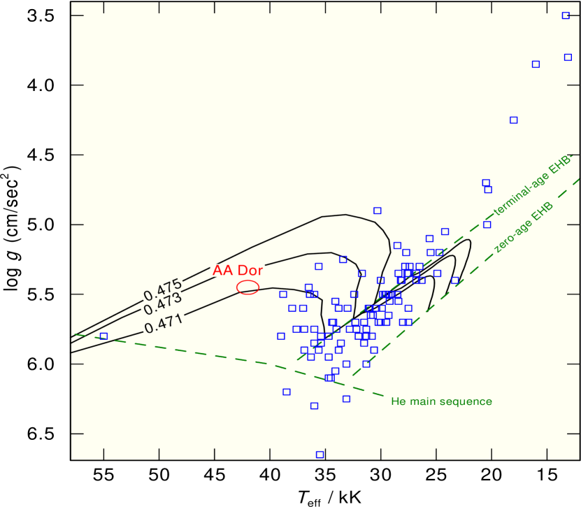
A mass of is determined by comparing of and with the evolutionary tracks of post-EHB stars (Fig. 6). From the same evolutionary calculations, we interpolate the primary’s luminosity. From our final model, we can determine the spectroscopic distance of AA Dor following Heber at al. (1984). We derive a distance of . The parameters of AA Dor are summarized in Tables 2 and 4.
4 Conclusions
The so-called problem in AA Dor is solved (Fig. 7) and our results (Table 4) are in good agreement with the photometric model of Hilditch et al. (2003).
Four influences were identified on the determination. 1) The major impact is the improvement in the Stark broadening tables, i.e. the difference between those of Lemke (1997) and of Tremblay & Bergeron (2009). This results in a systematic deviation of and . 2) The reflection effect is now eliminated by using only observed spectra that were obtained during the occultation of the secondary (Sect. 3). 3) The improved atomic data makes the model-atmosphere more reliable thanks to a fuller consideration of the metal-line blanketing. The temperature stratification of the stellar models, however, is only marginally affected. 4) The rotational velocity is lower than previously assumed (Müller et al. 2010). This only has little influence on the inner line core and is thus important for weak and narrow lines like He II Å (Fig. 1).
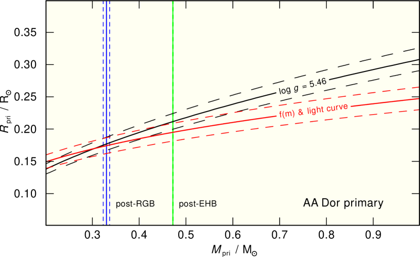
Since Vučković et al. (2008) identified spectral lines of the secondary in the UVES spectra and determined a lower limit () of its orbital velocity amplitude, both components’ masses are known (, , Vučković et al. 2008), albeit with large error bars. Müller et al. (2010) used the velocity amplitudes of both components (, ) to derive the masses and . This rules out a post-RGB scenario because post-RGB masses are significantly lower. The solution from mass function f(m) and light curve analysis, however, intersects with our result of (Fig. 7) even for the higher post-EHB mass (Fig. 6).
From our mass determination of , we calculated () the secondary’s mass of . Since the hydrogen-burning mass limit is about (Chabrier & Baraffe 1997; Chabrier et al. 2000), the secondary may either be a brown dwarf or a late M dwarf.
Acknowledgements.
We thank an anonymous referee, the editor R. Napiwotzki, and K. Werner for comments and discussions that helped to improve the paper. The UVES spectra used in this analysis were obtained as part of an ESO Service Mode run, proposal 66.D-1800. This research made use of the SIMBAD Astronomical Database, operated at the CDS, Strasbourg, France. We thank the GAVO team for support. TR is supported by the German Aerospace Center (DLR) under grant 05 OR 0806.References
- Asplund et al. (2009) Asplund, M., Grevesse, N., & Sauval, A. J. 2009, ARA&A, 47, 481
- Chabrier & Baraffe (1997) Chabrier, G., & Baraffe, I. 1997, A&A, 327, 1039
- Chabrier et al. (2000) Chabrier, G., Baraffe, I., Allard, F., & Hauschildt, P. 2000, ApJ, 542, 464
- Dorman et al. (1998) Dorman, B., Rood, R. T., & O’Connell, R. W. 1998, ApJ, 419, 596
- Edelmann (2003) Edelmann, H. 2003, PhD thesis, University Erlangen-Nuremberg, Germany
- Fleig et al. (2008) Fleig, J., Rauch, T., Werner, K., & Kruk, J. W. 2008, A&A, 492, 565
- Heber at al. (1984) Heber, U., Hunger, K., Jonas, G., & Kudritzki, R. P. 1984, A&A, 130, 119
- Hilditch et al. (1996) Hilditch, R. W., Harries, T. J., & Hill, G. 1996, MNRAS, 279, 1380
- Hilditch et al. (2003) Hilditch, R. W., Kilkenny, D., Lynas-Gray, A. E., & Hill, G. 2003, MNRAS, 344, 644
- Holweger (1979) Holweger, H. 1979, Les Elements et leurs Isotopes dans l’Universe, Université de Liège, Institute de Astrophysique, p. 117
- Hubeny et al. (1994) Hubeny, I., Hummer, D. G., & Lanz, T. 1994, A&A, 282, 151
- Hummer & Mihalas (1988) Hummer, D. G., & Mihalas, D. 1988, ApJ, 331, 794
- Kilkenny (2011) Kilkenny, D. 2011, MNRAS, 412, 487
- Kudritzki (1976) Kudritzki, R. P. 1976, A&A, 52, 11
- Kudritzki et al. (1982) Kudritzki, R. P., Simon, K. P., Lynas-Gray, A. E., Kilkenny, D., & Hill, P. W. 1982, A&A, 106, 254
- Kurucz (1991) Kurucz, R. L. 1991, in: Stellar Atmospheres: Beyond Classical Models, eds. L. Crivellari, I. Hubeny, D. G. Hummer, NATO ASI Series C, Vol. 341, Kluwer, Dordrecht, p. 441
- Kurucz (2009) Kurucz, R. L. 2009, in: Recent Directions in Astrophysical Quantitative Spectroscopy and Radiation Dynamics, eds. I. Hubeny, J. M. Stone, K. MacGregor, & K. Werner, AIP Conference Series Vol. 1171, p. 43
- Lemke (1997) Lemke, M. 1997, A&AS, 122, 285
- Müller et al. (2010) Müller, S., Geier, S., & Heber, U. 2010, Ap&SS, 329, 101
- Napiwotzki & Rauch (1994) Napiwotzki, R., & Rauch, T. 1994, A&A, 285, 603
- Rauch (2000) Rauch, T. 2000, A&A, 356, 665
- Rauch (2004) Rauch, T. 2004, Ap&SS, 291, 275
- Rauch & Deetjen (2003) Rauch, T., & Deetjen, J. L. 2003, in: Stellar Atmosphere Modeling, eds. I. Hubeny, D. Mihalas, K. Werner, The ASP Conference Series, Vol. 288, p. 103
- Rauch (1998) Rauch, T., Dreizler, S., & Wolff, B. 1998, A&A, 338, 651
- Repolust et al. (2005) Repolust, T., Puls, J., Hanson, M. M., Kudritzki, R.-P., & Mokiem, M. R. 2005, A&A, 440, 261
- Tremblay & Bergeron (2009) Tremblay, P.-E., & Bergeron, P. 2009, ApJ, 696, 1755
- Vučković et al. (2008) Vučković, M., Østensen, R., Bloemen, S., Decoster, I., & Aerts, C. 2008, in: Hot Subdwarf Stars and Related Objects, eds. U. Heber, C. S. Jeffery, R. Napiwotzki, The ASP Conference Series, Vol. 392, p. 199
- Werner (1996) Werner, K. 1996, ApJ, 457, L 39
- Werner et al. (2003) Werner, K., Dreizler, S., Deetjen, J. L., Nagel, T., Rauch, T., & Schuh, S. L. 2003, in: Stellar Atmosphere Modeling, eds. I. Hubeny, D. Mihalas, K. Werner, The ASP Conference Series, Vol. 288, p. 31