The asymptotic Bethe ansatz solution for one-dimensional $SU(2)$ spinor bosons with finite range Gaussian interactions

Abstract

We propose a one-dimensional model of spinor bosons with $SU(2)$ symmetry and a two-body finite range Gaussian interaction potential. We show that the model is exactly solvable when the width of the interaction potential is much smaller compared to the inter-particle separation. This model is then solved via the asymptotic Bethe ansatz technique. The ferromagnetic ground state energy and chemical potential are derived analytically. We also investigate the effects of a finite range potential on the density profiles through local density approximation. Finite range potentials are more likely to lead to quasi Bose-Einstein condensation than zero range potentials.

I Introduction

Integrable one-dimensional (1D) models of interacting bosons and fermions with $\delta$-function interaction Lieb1963 ; Yang1967 ; Gaudin1967 have had a tremendous impact on quantum statistical mechanics. In particular, recent breakthrough experiments on trapped ultracold bosons and fermions atoms confined to 1D have provided a better understanding of quantum statistical effects and strongly correlated phenomena in quantum many-body systems. These models contain two-body zero range potentials which allows the wavefunctions to be written as a superposition of plane waves by means of Bethe’s hypothesis Bethe1931 . This assumption is true based on the fact that every particle can move freely without feeling the presence of others when no collision takes place.

However, Calogero Calogero1969 showed that certain models with long range potentials can also be solved exactly, though not using Bethe’s hypothesis. He first solved the three-body problem with a harmonic potential and a $g/r^{2}$ potential, and then generalized it to the $N$-body problem to obtain the exact expression for the ground state energy and a class of excited states. Sutherland Sutherland1971 then derived the exact solutions for the ground state energy, pair correlation function, low-lying excitations and thermodynamics of the model with $g/r^{2}$ potential for both fermions and bosons in the thermodynamic limit by employing the asymptotic Bethe ansatz (ABA) which uses Bethe’s hypothesis in the asymptotic limit. Since then, many models with non-local interaction were solved exactly through the ABA method. Among them are the isotropic Heisenberg antiferromagnetic chain Haldane1988 , the quantum lattice model with inverse $\sinh$ square potential Sutherland1994 , the $t-J$ model with long range interaction Kawakami1992 , the nonliner Schrödinger model Kundu1993 and so on.

The main idea of the ABA is that one restricts oneself to the asymptotic region where the particles are considered to be sufficiently far apart, such that their influence on neighboring particles is negligible Sutherland . Then one has to show by some unspecified method that the system is integrable, i.e., that it has a complete set of independent integrals of motion. For example, various authors Moser1975 have shown that for $g/r^{2}$ potentials, one can find $N$ integrals of motion for the $N$ particle system. Once this is done, one can then conclude that the wavefunction is non-diffractive and thus asymptotically given by the BA. Since the exact scattering data is known, one can then obtain the exact thermodynamics of the system Sutherland1993 . It should be pointed out that a common misconception is that the ABA is only a low-density approximation, i.e., $N/L\rightarrow 0$. This is not true and in fact it gives the exact thermodynamics for systems with finite density in the thermodynamic limit (see Sutherland for explanations). When using the ABA, the low-density limit $N/L\rightarrow 0$ is only reached when the width of the interaction potential between neighboring particles become large. However, for the purpose of this investigation, we restrict ourselves to a finite density system where the width of the interaction potential between particles is small. A physical example of systems with such properties are dilute gases, whose inter-particle interactions are almost local.

In this paper, we investigate the ground state of two-component spinor bosons with finite range Gaussian interactions in 1D. The interaction potential for this system can be expressed in terms of the sum of even powered derivatives of a $\delta$-function. It gives rise to certain nonlinear behaviour not observed in systems with spin-independent potentials Batchelor2008 . This kind of velocity- or state-dependent potential leads to more versatility in studying spin waves, ferromagnetic behaviour and the relation between superfluidity and magnetism in low-dimensional many-body systems, as shown in Ref. Wicke2010 for two-component ⁸⁷Rb atoms on a quantum chip. By using a state-dependent dressed potential, spin degrees of freedom in two-component spinor bosons are tunable. This technique for controlling non-equilibrium spin motion allows one to study quantum coherence in interacting quantum systems, and to experimentally explore predictions of the thermodynamic Bethe Ansatz (TBA) in a system of two-component spinor bosons.

We first introduce the model in Section II. In Section III, we show that the Hamiltonian for this model is integrable. In Section IV, we derive the distribution functions for the charge and spin degrees of freedom from the ABA equations. The ground state energy and thermodynamics are evaluated in Section V in the limits where the interaction strength between particles is large and the width of the interaction potential is small. In Section VI, we apply the local density approximation to obtain the density profiles for this model. And finally in Section VII, we conclude with a summary of our results.

II The Model

Let us consider $N$ bosons with $SU(2)$ symmetry confined to a 1D wire of length $L$ with periodic boundary conditions. Here we denote the internal hyperfine spin states as $|\uparrow\rangle$ and $|\downarrow\rangle$. The interaction potential between adjacent particles is given by a generic non-negative function $v(x_{j}-x_{l})$ that is even in the inter-particle separation, i.e., $v(x)=v(-x)$ and vanishes at large enough distances, i.e., $\lim_{x\rightarrow\infty}v(x)=0$. For such a system, the first quantized Hamiltonian is given by

$$\mathcal{H}=-\frac{\hbar^{2}}{2m}\sum_{j=1}^{N}\frac{\partial^{2}}{\partial x_{j}^{2}}+2c\sum_{j<l}v(x_{j}-x_{l})-\frac{H}{2}(N_{\uparrow}-N_{\downarrow}),$$ (1)

where $m$ is the mass of each boson and $c$ characterizes the interaction strength which is the same for all possible collisions, i.e., between two $|\uparrow\rangle$ bosons, two $|\downarrow\rangle$ bosons, or one $|\uparrow\rangle$ and one $|\downarrow\rangle$ boson. The interactions are repulsive when $c>0$ and attractive when $c<0$. The external magnetic field is represented by $H$, and the total particle number is given by $N=N_{\uparrow}+N_{\downarrow}$. For the rest of this paper we use the dimensionless units of $\hbar=2m=1$ for convenience. These units are also used in all figures.

In the case when

$$v(x)=\frac{1}{\sqrt{2\pi\alpha^{2}}}\exp\left(-\frac{x^{2}}{2\alpha^{2}}\right),$$ (2)

the model can be exactly solved in the region $x_{1}\ll x_{2}\ll\ldots\ll x_{N}$ where the width of the Gaussian potential $\alpha$ is small relative to the inter-particle separation, i.e., $|x_{i+1}-x_{i}|\gg\alpha$ or $(N/L)\alpha\ll 1$ for every $i<N$. In this limit, all particles scatter non-diffractively. This implies that the asymptotic wavefunction can be written as a sum of $N!$ terms corresponding to the permutations $P$ of the set of asymptotic momenta $\{k_{i}\}$. Explicitly, the wavefunction can be expressed in Bethe ansatz form as

$$\psi(\mathbf{x})=\sum_{P}A(P)\exp\left(\mathrm{i}\sum_{j=1}^{N}k_{P_{j}}x_{j}\right).$$ (3)

The argument that supports non-diffractive scattering is as follows. Consider the two-body problem $N=2$ where the particles are far apart, i.e., $x_{1}\ll x_{2}$. Since $|x_{2}-x_{1}|\gg\alpha$, the particles behave as free particles, therefore the wavefunction is a product of plane waves with total momentum and energy given by

$$P=k_{1}+k_{2},\qquad E=k_{1}^{2}+k_{2}^{2}.$$ (4)

Through the scattering process, the total momentum and energy have to be conserved. This yields a new set of momenta which is either $(k_{1}^{\prime},k_{2}^{\prime})=(k_{1},k_{2})$ or $(k_{1}^{\prime},k_{2}^{\prime})=(k_{2},k_{1})$.

For the $N$-body problem, we can think of it as a succession of two particles colliding and then scattering to the asymptotic region as free particles, where each two-body collision gives rise to a permutation of the momenta. A product of transpositions acting on the permutation $P$ leads to another permutation $P^{\prime}$. Hence, the scattering is non-diffractive for any number of particles. When $\alpha\rightarrow 0$ in the fully polarized case, $v(x)\rightarrow\delta(x)$ which allows us to recover the Lieb-Liniger interacting spinless Bose gas Lieb1963 .

III Integrability of the Hamiltonian

We know that in the limit $\alpha\rightarrow 0$, the Gaussian function tends to the $\delta$-function. The $\delta$-function is not a function in the classical sense, and should be treated as a generalized function Gelfand1964 instead. Notice that if the potential $v(x)$ is an even function, its Fourier transform $\widehat{v}(k)=\int_{-\infty}^{\infty}v(x)e^{\mathrm{i}kx}dx$ is also an even function, i.e., $\widehat{v}(k)=\widehat{v}(-k)$. This implies that the Taylor expansion of $\widehat{v}(k)$ in the neighborhood of $k=0$ only consists of even powers of $k$ as given by

$$\widehat{v}(k)=\sum_{n=0}^{\infty}b_{n}k^{2n}.$$ (5)

Assuming that the potential meets such restrictions, we can take the inverse Fourier transform to obtain the potential in position space as

$$v(x) = \frac{1}{2\pi}\sum_{n=0}^{\infty}\int_{-\infty}^{\infty}b_{n}k^{2n}e^{-\mathrm{i}kx}dk$$ (6)

$$\equiv \sum_{n=0}^{\infty}a_{n}\delta^{(2n)}(x),$$

where $a_{n}=(-1)^{n}b_{n}$. This result is derived from the fact that the $2n$-th derivative of the $\delta$-function can be expressed as $\delta^{(2n)}(x)=\frac{1}{2\pi}\int_{-\infty}^{\infty}(-1)^{n}k^{2n}e^{-\mathrm{i}kx}$dk.

Let us now consider a Gaussian type potential. The Fourier transform of the Gaussian function is still a Gaussian function and is given by

$$F\left[\frac{1}{\sqrt{2\pi\alpha^{2}}}\exp\left(-\frac{x^{2}}{2\alpha^{2}}\right)\right]=\exp\left(-\frac{\alpha^{2}k^{2}}{2}\right).$$ (7)

The Taylor expansion of the right-hand side of Eq. (7) at $k=0$ is

$$\exp\left(-\frac{\alpha^{2}k^{2}}{2}\right)=\sum_{n=0}^{\infty}(-1)^{n}\frac{1}{n!}\left(\frac{\alpha^{2}}{2}\right)^{n}k^{2n}.$$ (8)

From Eqs. (5) and (6), we deduce that

$$v(x)=\frac{1}{\sqrt{2\pi\alpha^{2}}}\exp\left(-\frac{x^{2}}{2\alpha^{2}}\right)=\sum_{n=0}^{\infty}\frac{1}{n!}\left(\frac{\alpha^{2}}{2}\right)^{n}\delta^{(2n)}(x).$$ (9)

It seems a little odd at first glance that an analytic function can be written in the form of an infinite sum of generalized functions. We emphasize that this equality does not hold at isolated points, i.e., we cannot, for instance, say that the equality holds at the point $x_{0}$. But one can convince oneself that it holds whenever we consider $v(x)$ as a continuous linear functional that associates every function $\psi(x)$ which vanishes outside some bounded region and has continuous derivatives of all orders, a real number $(v,\psi)$. Mathematically, $v(x)$ is considered a functional in the sense that $(v,\psi)=\int_{R}v(x)\psi(x)dx$ where the integration is performed over the real line for this instance. One can also check the validity of the expansion $v(x)$ in terms of a linear combination of $\delta^{(2n)}(x)$, denoted as $v_{\delta}(x)$, when $\psi(\mathbf{x})=\sum_{P}A_{\sigma_{1}\ldots\sigma_{N}}(P|Q)\exp(\mathrm{i}\sum_{j=1}^{N}k_{P_{j}}x_{Q_{j}})$ is the Bethe ansatz wavefunction, by comparing the expressions of $(v,\psi)$ and $(v_{\delta},\psi)$. In Appendix A, we verify the claim that $(v,\psi)=(v_{\delta},\psi)$.

With this expression for the potential $v(x)$ and after verifying that $(v,\psi)=(v_{\delta},\psi)$, we can re-write the Hamiltonian in Eq. (1) as

$$\mathcal{H}=-\sum_{j=1}^{N}\frac{\partial^{2}}{\partial x_{j}^{2}}+2c\sum_{j<l}\sum_{n=0}^{\infty}\frac{1}{n!}\left(\frac{\alpha^{2}}{2}\right)^{n}\delta^{(2n)}(x_{j}-x_{l})-\frac{H}{2}(N_{\uparrow}-N_{\downarrow}).$$ (10)

Following Gutkin’s work Gutkin1987 , we can show that this Hamiltonian is integrable. The boundary condition imposed by Eq. (10) (derived in detail in Appendix C) is

$$\left(\frac{\partial}{\partial x_{j+1}}-\frac{\partial}{\partial x_{j}}\right)\psi|_{x_{j}=x_{j+1}^{+}}-\left(\frac{\partial}{\partial x_{j+1}}-\frac{\partial}{\partial x_{j}}\right)\psi|_{x_{j}=x_{j+1}^{-}}$$

$$\quad=2C\sum_{n=0}^{\infty}\frac{1}{n!}\left(\frac{\alpha^{2}}{8}\right)^{n}\left(\frac{\partial}{\partial x_{j+1}}-\frac{\partial}{\partial x_{j}}\right)^{2n}\psi|_{x_{j}=x_{j+1}}.$$ (11)

Here the interaction strength $C$ is now a $d\times d$ matrix, where $d$ represents the number of internal energy levels. More explicitly, $C=cI^{d}$ where $I^{d}$ is a $d\times d$ identity matrix. The superscripts $+$ and $-$ on the position of the $(j+1)$-th particle $x_{j}$ have the meaning that $x_{j+1}^{+(-)}$ is infinitesimally greater (or smaller) than $x_{j+1}$. This boundary condition is a specific case of the ones derived in Refs. Ord1989 ; Lai1995 for velocity dependent $\delta$-function potentials. To compute the matching coefficients $A(\lambda,\mu)$ and $B(\lambda,\mu)$ that are found in Ref. Gutkin1987 , we assume that the wavefunctions before collision and after collision are

$$\psi|_{x_{j}=x_{j+1}^{-}} = e^{\mathrm{i}(\lambda x_{j}+\mu x_{j+1})},$$ (12)

$$\psi|_{x_{j}=x_{j+1}^{+}} = A(\lambda,\mu)e^{\mathrm{i}(\lambda x_{j}+\mu x_{j+1})}+B(\lambda,\mu)e^{\mathrm{i}(\mu x_{j}+\lambda x_{j+1})}.$$ (13)

Next, we substitute these wavefunctions into Eq. (11) and use Proposition 1 in Ref. Gutkin1987 , i.e., $A(\lambda,\mu)+B(\lambda,\mu)=1$, which states that there are only two possible plane wave solutions after collision. These are either where (i) the momenta of scattering particles are interchanged, or (ii) the momenta of scattering particles are left unchanged, with the sum of their probabilities equal to 1. This yields the solutions for $A(\lambda,\mu)$ and $B(\lambda,\mu)$, i.e.,

$$A(\lambda,\mu) = \frac{(\lambda-\mu)-\mathrm{i}C\sum_{n=0}^{\infty}\frac{1}{n!}\left(-\frac{\alpha^{2}}{8}\right)^{n}(\lambda-\mu)^{2n}}{\lambda-\mu},$$ (14)

$$B(\lambda,\mu) = \frac{\mathrm{i}C\sum_{n=0}^{\infty}\frac{1}{n!}\left(-\frac{\alpha^{2}}{8}\right)^{n}(\lambda-\mu)^{2n}}{\lambda-\mu}.$$ (15)

From Theorem 2(b) in Ref. Gutkin1987 , the symmetric Bethe ansatz, i.e., Bethe’s hypothesis for a system of bosons, is satisfied since we have found a pair of commuting matching coefficients $A(\lambda,\mu)$ and $B(\lambda,\mu)$ for any matrix $C=cI^{d}$. Hence we have shown that this model is BA integrable. The $N$ particle symmetric wavefunction can then be expressed as

$$\psi(x_{Q_{1}}\ll x_{Q_{2}}\ll\ldots\ll x_{Q_{N}})=\sum_{P}A_{\sigma_{1}\ldots\sigma_{N}}(P|Q)\exp\left(\mathrm{i}\sum_{j=1}^{N}k_{P_{j}}x_{Q_{j}}\right).$$ (16)

This wavefunction is a superposition of plane waves with different amplitudes $A_{\sigma_{1}\ldots\sigma_{N}}(P|Q)$ (not to be confused with the coefficient $A(\lambda,\mu)$) where $P$ and $Q$ are permutations of the set of integers $\{1,2,\ldots,N\}$. Each plane wave is characterized by the permutation $P$ of wavenumbers $\{k_{j}\}$, therefore the sum contains $N!$ terms. Here $\sigma_{j}$’s represent the spin coordinates.

It should be noted that the simple procedure of replacing an analytic function by a linear combination of $2n$-th order derivatives of the $\delta$-function may lead one to think that any Hamiltonian with a pairwise interaction potential which is an even function can be exactly solved via the ABA. However, this is not true. The BA integrability conditions met by the Gaussian function is actually quite restrictive. First of all, any non-local potential we choose has to be well-behaved, smooth and an even function. Secondly, it has to vanish quickly as a function of the distance between neighboring particles in order for us to make use of the ABA. Thirdly, the Gaussian function is unique in the sense that it satisfies both previous conditions, and can still be reduced to a $\delta$-function as its width vanishes to zero. This third point enables us to make sure our results reduce to the Lieb-Liniger case in the limit $\alpha\rightarrow 0$, which is a necessary condition. These three points eliminate many candidates for a choice of pairwise interaction potential. In Appendix B, we show that for the case where $T=0$, there exists a unique solution for the Bethe roots, and that they are good quantum numbers.

IV The Ground State

The scattering matrix and the ABA equations for this model are derived in Appendix C and Appendix D. The ABA equations are given by

$$\exp(\mathrm{i}k_{j}L)=-\prod_{l=1}^{N}\frac{k_{j}-k_{l}+\mathrm{i}c^{\prime}(k_{j}-k_{l})}{k_{j}-k_{l}-\mathrm{i}c^{\prime}(k_{j}-k_{l})}\prod_{i=1}^{M}\frac{k_{j}-\lambda_{i}-\mathrm{i}c^{\prime}(k_{j}-\lambda_{i})}{k_{j}-\lambda_{i}},\qquad j=1,\ldots,N,$$ (17)

$$\prod_{l=1}^{N}\frac{\lambda_{i}-k_{l}+\mathrm{i}c^{\prime}(\lambda_{i}-k_{l})}{\lambda_{i}-k_{l}}=-\prod_{j=1}^{M}\frac{\lambda_{i}-\lambda_{j}+\mathrm{i}c^{\prime}(\lambda_{i}-\lambda_{j})}{\lambda_{i}-\lambda_{j}-\mathrm{i}c^{\prime}(\lambda_{i}-\lambda_{j})},\qquad i=1,\ldots,M.$$ (18)

where the effective interaction strength $c^{\prime}(u)=ce^{-\alpha^{2}u^{2}/8}$ is given in Eq. (85). Here, $M$ denotes the number of spin-down bosons in a system where the vacuum state (initial reference state) consists of $N$ spin-up bosons. The rapidities for the spin degrees of freedom are given by $\{\lambda_{i}\}$.

When $T=0$ there are no strings involved in the solution for $\{\lambda_{i}\}$, i.e., all $\lambda_{i}$’s are real. Taking the logarithm of the ABA equations gives

$$k_{j}L=2\pi I_{j}-\sum_{l=1}^{N}\theta\left(\frac{k_{j}-k_{l}}{c^{\prime}(k_{j}-k_{l})}\right)+\frac{1}{2}\sum_{i=1}^{M}\theta\left(\frac{k_{j}-\lambda_{i}}{c^{\prime}(k_{j}-\lambda_{i})}\right)+\sum_{i=1}^{M}\ln\sqrt{1+\left[\frac{c^{\prime}(k_{j}-\lambda_{i})}{k_{j}-\lambda_{i}}\right]^{2}},$$ (19)

$$\frac{1}{2}\sum_{l=1}^{N}\theta\left(\frac{\lambda_{i}-k_{l}}{c^{\prime}(\lambda_{i}-k_{l})}\right)-\sum_{l=1}^{N}\ln\sqrt{1+\left[\frac{c^{\prime}(\lambda_{i}-k_{l})}{\lambda_{i}-k_{l}}\right]^{2}}=2\pi J_{i}+\sum_{j=1}^{M}\theta\left(\frac{\lambda_{i}-\lambda_{j}}{c^{\prime}\lambda_{i}-\lambda_{j})}\right),$$ (20)

where $\theta(x)=2\tan^{-1}x$. Here, quantum numbers $I_{j}$ are integers (half-odd integers) when $N-M/2$ is odd (even) and $J_{i}$ are integers (half-odd integers) when $N/2-M$ is odd (even). Let us then define the functions $h(k)$ and $j(\lambda)$ to represent “particles” when $Lh(k)=2\pi I$ and when $Lj(\lambda)=2\pi J$. This yields

$$h(k) = k+\frac{1}{L}\sum_{l=1}^{N}\theta\left(\frac{k-k_{l}}{c^{\prime}(k-k_{l})}\right)-\frac{1}{2L}\sum_{i=1}^{M}\theta\left(\frac{k-\lambda_{i}}{c^{\prime}(k-\lambda_{i})}\right)$$ (21)

$$-\frac{1}{L}\sum_{i=1}^{M}\ln\sqrt{1+\left[\frac{c^{\prime}(k-\lambda_{i})}{k-\lambda_{i}}\right]^{2}},$$

$$j(\lambda) = \frac{1}{2L}\sum_{l=1}^{N}\theta\left(\frac{\lambda-k_{l}}{c^{\prime}(\lambda-k_{l})}\right)-\frac{1}{L}\sum_{j=1}^{M}\theta\left(\frac{\lambda-\lambda_{j}}{c^{\prime}(\lambda-\lambda_{j})}\right)$$ (22)

$$-\frac{1}{L}\sum_{l=1}^{N}\ln\sqrt{1+\left[\frac{c^{\prime}(\lambda-k_{l})}{\lambda-k_{l}}\right]^{2}}.$$

In the thermodynamic limit,

$$h(k) = k+\int\theta\left(\frac{k-k^{\prime}}{c^{\prime}(k-k^{\prime})}\right)\rho(k^{\prime})dk^{\prime}-\frac{1}{2}\int\theta\left(\frac{k-\lambda}{c^{\prime}(k-\lambda)}\right)\sigma(\lambda)d\lambda$$ (23)

$$-\int\ln\sqrt{1+\left[\frac{c^{\prime}(k-\lambda)}{k-\lambda}\right]^{2}}\sigma(\lambda)d\lambda,$$

$$j(\lambda) = \frac{1}{2}\int\theta\left(\frac{\lambda-k}{c^{\prime}(\lambda-k)}\right)\rho(k)dk-\int\theta\left(\frac{\lambda-\lambda^{\prime}}{c^{\prime}(\lambda-\lambda^{\prime})}\right)\sigma(\lambda^{\prime})d\lambda^{\prime}$$ (24)

$$-\int\ln\sqrt{1+\left[\frac{c^{\prime}(\lambda-k)}{\lambda-k}\right]^{2}}\rho(k)dk,$$

where $\rho(k)$ and $\sigma(\lambda)$ are the distribution functions for charge and spin degrees of freedom, respectively. There are no “holes” in the ground state, therefore we can safely take $\rho^{h}(k)=\sigma^{h}(\lambda)=0$. Define $\frac{d}{dk}h(k)=2\pi\rho(k)$ and $\frac{d}{dk}j(\lambda)=2\pi\sigma(\lambda)$. Taking the derivatives of Eqs. (23) and (24) finally leads to expressions for the distribution functions in the form

$$\rho(k) = \frac{1}{2\pi}+\int K_{1}(k-k^{\prime})\rho(k^{\prime})dk^{\prime}-\frac{1}{2}\int K_{1}(k-\lambda)\sigma(\lambda)d\lambda+\int K_{2}(k-\lambda)\sigma(\lambda)d\lambda,$$ (25)

$$\sigma(\lambda) = \frac{1}{2}\int K_{1}(\lambda-k)\rho(k)dk-\int K_{1}(\lambda-\lambda^{\prime})\sigma(\lambda^{\prime})d\lambda^{\prime}+\int K_{2}(\lambda-k)\rho(k)dk.$$ (26)

The functions $K_{1}(x)$ and $K_{2}(x)$ are given by

$$K_{1}(x) = \frac{1}{\pi}\frac{c^{\prime}(x)[1+\frac{\alpha^{2}}{4}x^{2}]}{[c^{\prime}(x)]^{2}+x^{2}},$$ (27)

$$K_{2}(x) = \frac{1}{2\pi}\frac{c^{\prime}(x)}{x}\frac{c^{\prime}(x)[1+\frac{\alpha^{2}}{4}x^{2}]}{[c^{\prime}(x)]^{2}+x^{2}}\equiv\frac{c^{\prime}(x)}{2x}K_{1}(x).$$ (28)

V The Thermodynamics in the Limits $c\gg 1$ and $\alpha\ll 1$

The model described by the Hamiltonian in Eq. (1) does not include any explicit spin-dependent forces. Therefore the ground state is ferromagnetic according to a theorem given by Eisenberg and Lieb Eisenberg2002 . When the external magnetic field $H>0$, the ground state is fully populated by $|\uparrow\rangle$ states which were the reference states that we used to derive the ABA equations. When $H<0$, all $|\uparrow\rangle$ states will flip into $|\downarrow\rangle$ states. The ferromagnetic behavior and thermodynamics of the special case $\alpha=0$ has been studied in literature Guan2007 ; Caux2009 .

When $T=0$ and $H>0$, our model reduces to the single component case. Here $\sigma(\lambda)=0$ since the distribution of $|\downarrow\rangle$ is zero. Therefore we only have one equation to solve

$$\rho(k)=\frac{1}{2\pi}+\int_{-Q}^{Q}\frac{1}{\pi}\frac{c^{\prime}(k-k^{\prime})[1+\frac{\alpha^{2}}{4}(k-k^{\prime})^{2}]}{[c^{\prime}(k-k^{\prime})]^{2}+(k-k^{\prime})^{2}}\rho(k^{\prime})dk^{\prime},$$ (29)

where $\pm Q$ are the “Fermi” points. In FIG. 1 and FIG. 2, we plot $\rho(k)$ versus $k$ for different values of $c$ and $\alpha$ by numerically solving Eq. (29). In both figures, we consider values of $\alpha$ and $c$ that are beyond the ABA regime, i.e., values that are outside the limits $\alpha\ll 1$ and $c\gg 1$. This is done so that we can more easily visualize how the distribution function $\rho(k)$ varies as both parameters vary. We stress that the curves in FIG. 1 and FIG. 2 become less accurate as $\alpha$ tends to larger values or as $c$ tends to smaller values. It is clear from the figures that as the interaction width $\alpha$ increases, the distribution of quasimomenta $k$ become more centered around the origin. This is because the increase in overlap between single particle wavefunctions causes the system to behave more and more like a Bose-Einstein condensate where the quasimomenta of particles occupy a smaller region in momentum space.

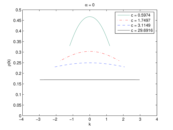
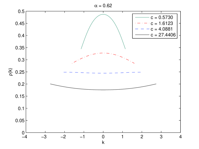
Figure 1: (Color online) Plots of $\rho(k)$ versus $k$ for different values of $c$, with fixed density $n=1$. The top graph has a value of $\alpha=0$ (where one recovers the Lieb-Liniger Bose gas) and the bottom graph has a value of $\alpha=0.62$. All curves are obtained by numerically solving Eq. (29).

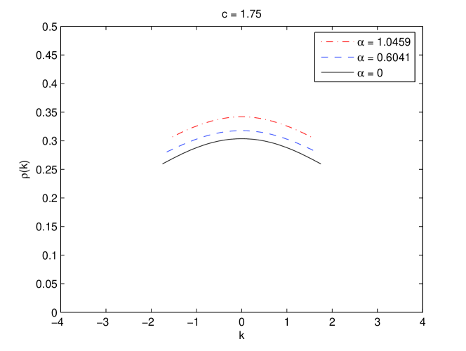
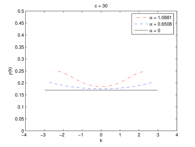
Figure 2: (Color online) Numerical plots of $\rho(k)$ versus $k$ for different values of $\alpha$, with fixed density $n=1$. The top graph has a value of $c=1.75$ and the bottom graph has a value of $c=30$. All curves are obtained by numerically solving Eq. (29).

Using the relations $n=\int_{-Q}^{Q}\rho(k)dk$ and $E/L=\int_{-Q}^{Q}k^{2}\rho(k)dk$, we can approximate $\rho(k)$ by using Taylor’s expansion to get

$$\rho(k) = \frac{1}{2\pi}+\int_{-Q}^{Q}\frac{1}{\pi}\frac{ce^{-\alpha^{2}(k-k^{\prime})^{2}/8}[1+\frac{\alpha^{2}}{4}(k-k^{\prime})^{2}]}{c^{2}e^{-\alpha^{2}(k-k^{\prime})^{2}/4}+(k-k^{\prime})^{2}}\rho(k^{\prime})dk^{\prime}$$ (30)

$$= \frac{1}{2\pi}+\frac{1}{\pi c}\int_{-Q}^{Q}\left(1+\frac{3\alpha^{2}}{8}(k-k^{\prime})^{2}+\frac{5\alpha^{4}}{128}(k-k^{\prime})^{4}-\ldots\right)\rho(k^{\prime})dk^{\prime}$$

$$= \frac{1}{2\pi}+\frac{1}{\pi c}\left(1+\frac{3\alpha^{2}}{8}k^{2}+\frac{5\alpha^{4}}{128}k^{4}\right)\int_{-Q}^{Q}\rho(k^{\prime})dk^{\prime}+\frac{1}{\pi c}\left(\frac{3\alpha^{2}}{8}+\frac{15\alpha^{4}}{64}k^{2}\right)\int_{-Q}^{Q}k^{\prime 2}\rho(k^{\prime})dk^{\prime}$$

$$+\frac{5\alpha^{4}}{128\pi c}\int_{-Q}^{Q}k^{\prime 4}\rho(k^{\prime})dk^{\prime}+\ldots$$

$$= \frac{1}{2\pi}+\frac{n}{\pi c}\left(1+\frac{3\alpha^{2}}{8}k^{2}+\frac{5\alpha^{4}}{128}k^{4}\right)+\frac{3E\alpha^{2}}{8\pi Lc}\left(1+\frac{5\alpha^{2}}{8}k^{2}\right)+\frac{Q^{5}\alpha^{4}}{128\pi^{2}c}\left(1+\frac{2n}{c}\right)$$

$$+O\left(\frac{1}{c^{3}}\right)+O\left(\alpha^{6}\right).$$

The expression $\int_{-Q}^{Q}k^{\prime 4}\rho(k^{\prime})dk^{\prime}$ was evaluated by substituting the dominant terms in $\rho(k^{\prime})$ into the integral, which gave

$$\int_{-Q}^{Q}k^{4}\rho(k)dk\approx\int_{-Q}^{Q}k^{4}\left(\frac{1}{2\pi}+\frac{n}{\pi c}\right)dk=\frac{Q^{5}}{5\pi}\left(1+\frac{2n}{c}\right).$$ (31)

To find an expression for the Fermi point $Q$, we evaluate the integral

$$n = \int_{-Q}^{Q}\rho(k)dk$$

$$\approx \frac{Q}{\pi}\left[1+\frac{2n}{c}+\frac{3E\alpha^{2}}{4Lc}+\frac{nQ^{2}\alpha^{2}}{4c}+\frac{Q^{5}\alpha^{4}}{64\pi c}\left(1+\frac{2n}{c}\right)+\frac{5EQ^{2}\alpha^{4}}{32Lc}+\frac{nQ^{4}\alpha^{4}}{64c}\right].$$

Hence

$$Q = \pi n\left[1-\frac{2n}{c}\left(1-\frac{2n}{c}\right)-\frac{\pi^{2}n^{3}\alpha^{2}}{4c}\left(1-\frac{8n}{c}\right)-\frac{3E\alpha^{2}}{4Lc}\left(1-\frac{4n}{c}-\frac{3E\alpha^{2}}{4Lc}\right)\right.$$ (32)

$$\left.-\frac{\pi^{4}n^{5}\alpha^{4}}{32c}\left(1-\frac{14n}{c}\right)-\frac{5\pi^{2}n^{2}E\alpha^{4}}{32Lc}\left(1-\frac{44n}{5c}\right)\right]+O\left(\frac{1}{c^{3}}\right)+O\left(\alpha^{6}\right).$$

The ground state energy per unit length of the system is given by

$$\frac{E}{L} = \int_{-Q}^{Q}k^{2}\rho(k)dk$$ (33)

$$= \frac{Q^{3}}{3\pi}\left[1+\frac{2n}{c}+\frac{Q^{3}\alpha^{2}}{4\pi c}\left(1+\frac{2n}{c}\right)+\frac{9nQ^{2}\alpha^{2}}{20c}+\frac{Q^{6}\alpha^{4}}{16\pi^{2}c^{2}}+\frac{7Q^{5}\alpha^{4}}{64\pi c}\left(1+\frac{106n}{35c}\right)\right.$$

$$\left.+\frac{15nQ^{4}\alpha^{4}}{448c}\right]+O\left(\frac{1}{c^{3}}\right)+O\left(\alpha^{6}\right).$$

Substituting $Q$ into $E/L$ and collecting similar terms yields

$$\frac{E}{L} = \frac{1}{3}\pi^{2}n^{3}\left[1-\frac{4}{\gamma}\left(1-\frac{3}{\gamma}\right)-\frac{4\pi^{2}n^{2}\alpha^{2}}{5\gamma}\left(1-\frac{10}{\gamma}\right)-\frac{3\pi^{4}n^{4}\alpha^{4}}{28\gamma}\left(1+\frac{21}{10\gamma}\right)\right]$$ (34)

$$+O\left(\frac{1}{\gamma^{3}}\right)+O\left(\alpha^{6}\right).$$

where $\gamma=c/n$. With this expression for $E/L$, the “Fermi” points can be written explicitly as

$$Q=\pi n\left[1-\frac{2}{\gamma}\left(1-\frac{2}{\gamma}\right)-\frac{\pi^{2}n^{2}\alpha^{2}}{2\gamma}\left(1-\frac{8}{\gamma}\right)-\frac{\pi^{4}n^{4}\alpha^{4}}{12\gamma}\left(1-\frac{82}{5\gamma}\right)\right]+O\left(\frac{1}{\gamma^{3}}\right)+O\left(\alpha^{6}\right).$$ (35)

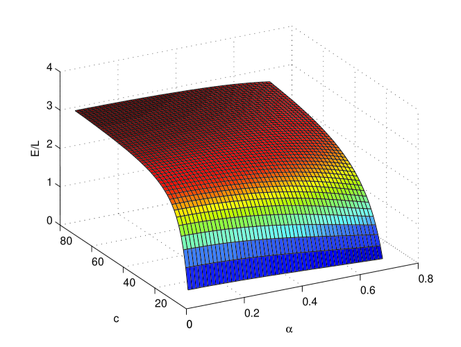
Figure 3: (Color online) Plot of the ground state energy per unit length $E/L$ versus the interaction width $\alpha$ and the interaction strength $c$ for a fixed density $n=1$. The surface is generated by numerically solving the equation $E/L=\int_{-Q}^{Q}k^{2}\rho(k)dk$.

With the expression for the ground state energy, the chemical potential can be derived using the relation

$$\mu = \frac{\partial}{\partial n}\left(\frac{E}{L}\right)$$ (36)

$$= \pi^{2}n^{2}\left[1-\frac{16}{3\gamma}\left(1-\frac{15}{4\gamma}\right)-\frac{8\pi^{2}n^{2}\alpha^{2}}{5\gamma}\left(1-\frac{35}{3\gamma}\right)-\frac{2\pi^{4}n^{4}\alpha^{4}}{7\gamma}\left(1+\frac{189}{80\gamma}\right)\right]$$

$$+O\left(\frac{1}{\gamma^{3}}\right)+O\left(\alpha^{6}\right).$$

The ground state energy is also calculated numerically for different values of $\alpha$ and $c$ by using $\rho(k)$ in Eq. (29) and the definition $E/L=\int_{-Q}^{Q}k^{2}\rho(k)dk$. We thus show a plot of $E/L$ versus $\alpha$ and $c$ in FIG. 3. As $c$ tends to infinity, the ground state energy will approach $\pi^{2}n^{3}/3$ as predicted by our analytical results. In FIG. 4, we compare our analytical solution given in Eq. (34) with the numerical solution for the ground state energy per unit length $E/L$ when $\alpha=0.1279$ and $n=1$. It is clear they both agree well when $c$ is large.

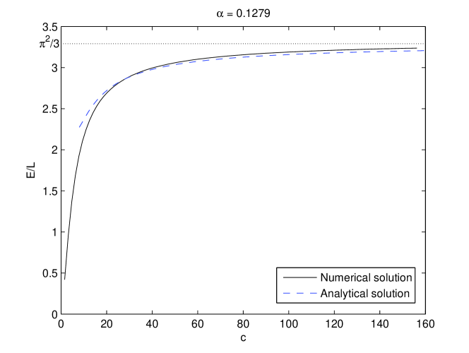
Figure 4: (Color online) Comparison between the analytical results and the numerical results for the ground state energy per unit length $E/L$ versus $c$ with $\alpha=0.1279$ and $n=1$.

VI Local Density Approximation

In this section, we explore the axial density when the system is confined by an external harmonic trapping potential. So far our application of the ABA to solve this model has been limited to the case where there is no external confinement. When an external confinement is applied, the model is no longer exactly solvable. However, if the external trapping potential varies slowly enough, the local density approximation (LDA) Dunjko2001 can be applied to analyze the density profiles in a harmonic trap.

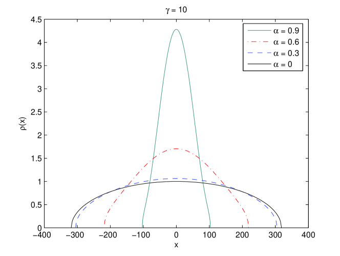
Figure 5: (Color online) Axial density profiles from the local density approximation for different values of $\alpha$. Here $\gamma=10$, total particle number $N=1000$, and the density at the center of the trap is taken to be $n(0)=1$.

In the LDA, the chemical potential varies along the axial direction $x$ according to the equation

$$\mu(x)=\mu(0)-\frac{m\omega^{2}x^{2}}{2}.$$ (37)

Using the result in Eq. (36), we then have

$$\mu(0)-\frac{m\omega^{2}x^{2}}{2} = \pi^{2}n(x)^{2}\left[1-\frac{16}{3\gamma}\left(1-\frac{15}{4\gamma}\right)-\frac{8\pi^{2}n(x)^{2}\alpha^{2}}{5\gamma}\left(1-\frac{35}{3\gamma}\right)\right.$$ (38)

$$\left.-\frac{2\pi^{4}n(x)^{4}\alpha^{4}}{7\gamma}\left(1+\frac{189}{80\gamma}\right)\right].$$

Solving this equation for $n(x)$ gives

$$n(x) = n(0)\sqrt{1-\frac{x^{2}}{R^{2}}}\left[1+\frac{4\pi^{2}n(0)^{2}\alpha^{2}}{5\gamma}\left(1-\frac{19}{3\gamma}\right)\left(1-\frac{x^{2}}{R^{2}}\right)\right.$$ (39)

$$\left.+\frac{\pi^{4}n(0)^{4}\alpha^{4}}{7\gamma}\left(1+\frac{28051}{1200\gamma}\right)\left(1-\frac{x^{2}}{R^{2}}\right)^{2}\right],$$

where

$$n(0)=\frac{1}{\pi}\sqrt{\frac{\mu(0)}{1-\frac{16}{3\gamma}(1-\frac{15}{4\gamma})}},$$ (40)

and

$$R^{2}=\frac{2\mu(0)}{m\omega^{2}}.$$ (41)

To obtain the density profiles, we solve the integral

$$\int_{-R}^{R}n(x)dx=N$$ (42)

numerically with total number $N=1000$ particles and particle density $n(0)=1$ at the center of the trap.

In FIG. 5, we show the axial density profiles for different values of $\alpha$. As the interaction width $\alpha$ increases, the particles become more concentrated at the center of the trap in a way analogous to a Bose-Einstein condensate.

VII Conclusion

In this paper, we studied a system of interacting $SU(2)$ spinor bosons in one-dimension with finite range Gaussian potential. Using Gutkin’s argument Gutkin1987 , this model is shown to be exactly solvable. We applied the asymptotic Bethe ansatz to solve this model when the interaction width $\alpha$ is much smaller than the inter-particle separation $|x_{i}-x_{j}|$. The Bethe ansatz equations were derived in Eqs. (17) and (18) through the quantum inverse scattering method. We went on to derive the particle distribution functions for the charge and spin degrees of freedom in Eqs. (25) and (26). In the limits $c\gg 1$, $\alpha\ll 1$ and $H>0$, we derived the ground state energy (34) and chemical potential (36) for the system. The spin independent interaction leads to a ferromagnetic ground state. Our analytical results were shown to be consistent with the exact numerical results from the asymptotic Bethe ansatz equations. Finally, we applied the local density approximation to analyze the density profiles of the system in an harmonic trapping potential. From our results, we showed that an increase in interaction width $\alpha$ causes the spatial and momentum density profiles of the system to more closely resemble that of a Bose-Einstein condensate, in the sense that density profiles are more concentrated around the origin.

This work has been partially supported by the Australian Research Council.

Appendix A Proof of $(v,\psi)=(v_{\delta},\psi)$

Given the Bethe ansatz wavefunction $\psi(\mathbf{x})=\sum_{P}A_{\sigma_{1}\ldots\sigma_{N}}(P|Q)\exp(\mathrm{i}\sum_{j=1}^{N}k_{P_{j}}x_{Q_{j}})$, it is straightforward to show that

$$(v,\psi) = \int_{-\infty}^{\infty}\frac{1}{\sqrt{2\pi\alpha^{2}}}e^{-x_{Q_{i}}^{2}/2\alpha^{2}}\sum_{P}A_{\sigma_{1}\ldots\sigma_{N}}(P|Q)\exp\left(\mathrm{i}\sum_{j=1}^{N}k_{P_{j}}x_{Q_{j}}\right)dx_{Q_{i}}$$ (43)

$$= \sum_{P}A_{\sigma_{1}\ldots\sigma_{N}}(P|Q)\exp\left(\mathrm{i}\sum_{j\neq i}^{N}k_{P_{j}}x_{Q_{j}}\right)F\left[\frac{1}{\sqrt{2\pi\alpha^{2}}}\exp\left(-\frac{x_{Q_{i}}^{2}}{2\alpha^{2}}\right)\right]$$

$$= \sum_{P}A_{\sigma_{1}\ldots\sigma_{N}}(P|Q)\exp\left(\mathrm{i}\sum_{j\neq i}^{N}k_{P_{j}}x_{Q_{j}}\right)\exp\left(-\frac{\alpha^{2}k^{2}_{P_{i}}}{2}\right),$$

and

$$(v_{\delta},\psi) = \int_{-\infty}^{\infty}\sum_{n=0}^{\infty}\frac{1}{n!}\left(\frac{\alpha^{2}}{2}\right)^{n}\delta^{(2n)}(x_{Q_{i}})\sum_{P}A_{\sigma_{1}\ldots\sigma_{N}}(P|Q)\exp\left(\mathrm{i}\sum_{j=1}^{N}k_{P_{j}}x_{Q_{j}}\right)dx_{Q_{i}}$$ (44)

$$= \sum_{P}A_{\sigma_{1}\ldots\sigma_{N}}(P|Q)\exp\left(\mathrm{i}\sum_{j\neq i}^{N}k_{P_{j}}x_{Q_{j}}\right)F\left[\sum_{n=0}^{\infty}\frac{1}{n!}\left(\frac{\alpha^{2}}{2}\right)^{n}\delta^{(2n)}(x_{Q_{i}})\right]$$

$$= \sum_{P}A_{\sigma_{1}\ldots\sigma_{N}}(P|Q)\exp\left(\mathrm{i}\sum_{j\neq i}^{N}k_{P_{j}}x_{Q_{j}}\right)\sum_{n=0}^{\infty}\frac{1}{n!}\left(\frac{\alpha^{2}}{2}\right)^{n}(-1)^{n}k_{P_{i}}^{2n}$$

$$= \sum_{P}A_{\sigma_{1}\ldots\sigma_{N}}(P|Q)\exp\left(\mathrm{i}\sum_{j\neq i}^{N}k_{P_{j}}x_{Q_{j}}\right)\exp\left(-\frac{\alpha^{2}k^{2}_{P_{i}}}{2}\right),$$

which verifies the claim that $(v,\psi)=(v_{\delta},\psi)$.

Appendix B Yang-Yang variational principle

Let us focus on repulsive potentials such that $v(x)$ is positive definite and $c>0$. When $T=0$, Eqs. (19) and (20) reduce to

$$k_{j}L=2\pi I_{j}-\sum_{l=1}^{N}2\tan^{-1}\left(\frac{k_{j}-k_{l}}{c\tilde{v}(k_{j}-k_{l})}\right),$$ (45)

where $I_{j}$ is an integer and $\tilde{v}(k)$ is the Fourier transform of $v(x)$. This is the fundamental equation for the Bethe roots which can be posed as a variational principle as shown by Yang and Yang for spinless bosons YangYang1969 . In order to show that Eq. (45) can be uniquely parameterized, we introduce the action

$$B(k_{1},\dots,k_{N})=\frac{L}{2}\sum_{j=1}^{N}k_{j}^{2}-2\pi I_{j}k_{j}+\sum_{j<l}\Phi(k_{j}-k_{l})$$ (46)

with

$$\Phi(x)=\int_{0}^{x}2\tan^{-1}\left(\frac{x^{\prime}}{c\tilde{v}(x^{\prime})}\right)dx^{\prime}.$$ (47)

Then we need to show that Eq. (45) is given by the minima condition

$$\frac{\partial B(k_{1},\dots,k_{N})}{\partial k_{j}}=0.$$ (48)

To prove this, we further introduce the $N\times N$ matrix

$$B_{jl}=\frac{\partial^{2}B}{\partial k_{j}\partial k_{l}} = \delta_{jl}\left[L+2c\sum_{m}\frac{\vartheta(k_{j}-k_{m})}{c^{2}\tilde{v}^{2}(k_{j}-k_{m})+(k_{j}-k_{m})^{2}}\right]$$ (49)

$$-2c\frac{\vartheta(k_{j}-k_{l})}{c^{2}\tilde{v}^{2}(k_{j}-k_{l})+(k_{j}-k_{l})^{2}}$$

which is always positive provided that

$$\vartheta(k)=\tilde{v}(k)-k\tilde{v}^{\prime}(k)>0.$$ (50)

If that is the case

$$\sum_{lj}u_{l}B_{lj}u_{j}=L\sum_{l}u_{l}^{2}+\sum_{l<j}c\frac{\vartheta(k_{j}-k_{l})}{c^{2}\tilde{v}^{2}(k_{j}-k_{l})+(k_{j}-k_{l})^{2}}(u_{j}-u_{l})^{2}\geq 0,$$ (51)

for arbitrary real $\{u_{j}\}$. Hence, the solutions of the fundamental equation exist and can be uniquely parameterized by a set of integer or half-integer numbers $I_{j}$, as long as $\vartheta(k)=\tilde{v}(k)-k\tilde{v}^{\prime}(k)\geq 0$.

We shall exclusively consider such type of potentials. Then, the Bethe roots are real numbers from Theorem I on p. 11 of Ref. Korepin . Finally if $I_{l}>I_{m}$ then $k_{l}>k_{m}$ and if $I_{l}=I_{m}$ then $k_{l}=k_{m}$ as long as $\tan^{-1}\left(k/c\tilde{v}(k)\right)$ increases monotonically with $k$. For the Gaussian potential, $\tilde{v}(k)=\exp(-\alpha^{2}k^{2}/2)$, which gives $\vartheta(k)=\tilde{v}(k)-k\tilde{v}^{\prime}(k)=\tilde{v}(k)(1+\alpha^{2}k^{2})>0$ for all real $k$. Therefore, there is a unique solution for the BA equations when the Gaussian potential is used.

Appendix C Derivation of the Scattering Matrix

We employ the coordinate BA to obtain the scattering matrix between two particles. This technique is well known, as used by Yang Yang1967 in solving the spin-1/2 fermion model. First consider the region

$$R:\quad 0\ll x_{Q_{1}}\ll\ldots\ll x_{Q_{j}}\ll x_{Q_{j+1}}\ll\ldots\ll x_{Q_{N}}\ll L.$$ (52)

Define a wavefunction in $R$ as

$$\psi(\mathbf{x})=\sum_{P}A_{\sigma_{1}\ldots\sigma_{N}}(P|Q)\exp\mathrm{i}(k_{P_{1}}x_{Q_{1}}+\ldots+k_{P_{j}}x_{Q_{j}}+k_{P_{j+1}}x_{Q_{j+1}}+\ldots+k_{P_{N}}x_{Q_{N}}),$$ (53)

where $\sigma_{j}$s represent the spin coordinates. This wavefunction is a superposition of plane waves with different amplitudes $A_{\sigma_{1}\ldots\sigma_{N}}(P|Q)$ where $P$ and $Q$ are permutations of the set of integers $\{1,2,\ldots,N\}$. Each plane wave is characterized by the permutation $P$ of wavenumbers $\{k_{j}\}$, therefore the sum contains $N!$ terms.

Consider a new region $R^{\prime}$ where particles at position $x_{Q_{j}}$ and $x_{Q_{j+1}}$ are interchanged, i.e.,

$$R^{\prime}:\quad 0\ll x_{Q_{1}}\ll\ldots\ll x_{Q_{j+1}}\ll x_{Q_{j}}\ll\ldots\ll x_{Q_{N}}\ll L.$$ (54)

In this region, the wavefunction is defined as

$$\psi^{\prime}(\mathbf{x})=\sum_{P}A_{\sigma_{1}\ldots\sigma_{N}}(P|Q^{\prime})\exp\mathrm{i}(k_{P_{1}}x_{Q_{1}}+\ldots+k_{P_{j}}x_{Q_{j+1}}+k_{P_{j+1}}x_{Q_{j}}+\ldots+k_{P_{N}}x_{Q_{N}}).$$ (55)

From the condition that the wavefunction has to be continuous when $x_{Q_{j}}\rightarrow x_{Q_{j+1}}$, we have the relation

$$A_{\sigma_{1}\ldots\sigma_{N}}(P|Q)+A_{\sigma_{1}\ldots\sigma_{N}}(P^{\prime}|Q)=A_{\sigma_{1}\ldots\sigma_{N}}(P|Q^{\prime})+A_{\sigma_{1}\ldots\sigma_{N}}(P^{\prime}|Q^{\prime}).$$ (56)

where $P^{\prime}$ and $Q^{\prime}$ represent the permutations $P^{\prime}=(j\phantom{ab}j+1)P$ and $Q^{\prime}=(j\phantom{ab}j+1)Q$, i.e., only the positions of the $j$-th and $(j+1)$-th terms are transposed to get $P^{\prime}$ from $P$, and $Q^{\prime}$ from $Q$.

The $\delta$-function potential gives rise to a jump in the first derivative of the wavefunction at position $x_{Q_{j}}=x_{Q_{j+1}}$. This jump can be evaluated by considering the Hamiltonian in the center of mass frame. In this frame, the new coordinates $X$ and $Y$ are related to the original coordinates $x_{j}$ and $x_{j+1}$ by the transformation relations

$$X=\frac{x_{j}+x_{j+1}}{2},\qquad Y=x_{j+1}-x_{j},$$ (57)

and

$$x_{j}=X-\frac{Y}{2},\qquad x_{j+1}=X+\frac{Y}{2}.$$ (58)

Their derivatives are related by

$$\frac{\partial}{\partial x_{j}}=\frac{1}{2}\frac{\partial}{\partial X}-\frac{\partial}{\partial Y},\qquad\frac{\partial}{\partial x_{j+1}}=\frac{1}{2}\frac{\partial}{\partial X}+\frac{\partial}{\partial Y},$$ (59)

and

$$\frac{\partial}{\partial X}=\frac{\partial}{\partial x_{j}}+\frac{\partial}{\partial x_{j+1}},\qquad\frac{\partial}{\partial Y}=\frac{1}{2}\left(\frac{\partial}{\partial x_{j+1}}-\frac{\partial}{\partial x_{j}}\right).$$ (60)

Higher order derivatives can be similarly expressed in a straightforward manner.

The time-independent Schrödinger equation $\mathcal{H}\psi=E\psi$ in these new coordinates is then given by

$$\left\{-\frac{1}{2}\frac{\partial^{2}}{\partial X^{2}}-2\frac{\partial^{2}}{\partial Y^{2}}+2c\sum_{n=0}^{\infty}\frac{1}{n!}\left(\frac{\alpha^{2}}{2}\right)^{n}\delta^{(2n)}(Y)+\ldots\right\}\psi(X,Y,\mathbf{x^{\prime}})=E\psi(X,Y,\mathbf{x^{\prime}}).$$ (61)

where the new set of coordinates $X$, $Y$ and $\mathbf{x^{\prime}}$ replace the old one $\mathbf{x}$. Also, the dimension of $\mathbf{x^{\prime}}$ is less than the dimension of $\mathbf{x}$ by two, since we replaced those two coordinates by $X$ and $Y$. Integrating this equation with respect to the $Y$ coordinate from $-\epsilon$ to $\epsilon$ and then taking $\epsilon\rightarrow 0$ gives

$$\left.\frac{\partial\psi}{\partial Y}\right|_{Y=0^{+}}-\left.\frac{\partial\psi}{\partial Y}\right|_{Y=0^{-}}=c\sum_{n=0}^{\infty}\frac{1}{n!}\left(\frac{\alpha^{2}}{2}\right)^{n}\left.\frac{\partial^{2n}\psi}{\partial Y^{2n}}\right|_{Y=0},$$ (62)

where we have repeatedly used integration by-parts to obtain the right hand side of the equation.

In the new coordinates, the wavefunctions given in Eqs. (53) and (55) are explicitly written as

$$\psi(X,Y,\mathbf{x^{\prime}})=\sum_{P}A_{\sigma_{1}\ldots\sigma_{N}}(P|Q)\exp\mathrm{i}\left(\ldots+(k_{P_{j}}+k_{P_{j+1}})X+\frac{1}{2}(k_{P_{j+1}}-k_{P_{j}})Y+\ldots\right),$$ (63)

and

$$\psi^{\prime}(X,Y,\mathbf{x^{\prime}})=\sum_{P}A_{\sigma_{1}\ldots\sigma_{N}}(P|Q^{\prime})\exp\mathrm{i}\left(\ldots+(k_{P_{j}}+k_{P_{j+1}})X-\frac{1}{2}(k_{P_{j+1}}-k_{P_{j}})Y+\ldots\right).$$ (64)

Substituting the wavefunctions defined in Eqs. (63) and (64) into Eq. (62) separately, and then adding both equations together yields the relation

$$\frac{\mathrm{i}}{2}(k_{P_{j+1}}-k_{P_{j}})\left[A_{\sigma_{1}\ldots\sigma_{N}}(P|Q)-A_{\sigma_{1}\ldots\sigma_{N}}(P^{\prime}|Q)\right]$$ (65)

$$+\hbox to0.0pt{$\displaystyle\frac{\mathrm{i}}{2}(k_{P_{j+1}}-k_{P_{j}})\left[A_{\sigma_{1}\ldots\sigma_{N}}(P|Q^{\prime})-A_{\sigma_{1}\ldots\sigma_{N}}(P^{\prime}|Q^{\prime})\right]$\hss}$$

$$=c\sum_{n=0}^{\infty}\frac{1}{n!}\left(\frac{\alpha^{2}}{2}\right)^{n}\left[\frac{\mathrm{i}}{2}(k_{P_{j+1}}-k_{P_{j}})\right]^{2n}\left[A_{\sigma_{1}\ldots\sigma_{N}}(P|Q)-A_{\sigma_{1}\ldots\sigma_{N}}(P^{\prime}|Q)\right].$$

We introduce the transposition operator $T_{i,j}$ which transposes the $i$th and $j$th spatial coordinates of the wavefunction, i.e.,

$$A_{\sigma_{1}\ldots\sigma_{N}}(\ldots P_{i}\ldots P_{j}\ldots|\ldots Q_{j}\ldots Q_{i}\ldots)$$ (66)

$$=\left[T_{i,j}\right]^{\sigma^{\prime}_{1}\ldots\sigma^{\prime}_{N}}_{\sigma_{1}\ldots\sigma_{N}}A_{\sigma^{\prime}_{1}\ldots\sigma^{\prime}_{N}}(\ldots P_{i}\ldots P_{j}\ldots|\ldots Q_{i}\ldots Q_{j}\ldots).$$

In matrix form, this operator $T_{i,j}$ can be written as $\left[T_{i,j}\right]^{\sigma^{\prime}_{1}\ldots\sigma^{\prime}_{N}}_{\sigma_{1}\ldots\sigma_{N}}=\pm\delta_{\sigma_{i},\sigma^{\prime}_{j}}\delta_{\sigma_{j},\sigma^{\prime}_{i}}\prod_{r\neq i,j}\delta_{\sigma_{r},\sigma^{\prime}_{r}}$, i.e., $T_{i,j}=\mathcal{P}_{i,j}$ for bosons and $T_{i,j}=-\mathcal{P}_{i,j}$ for fermions where $\mathcal{P}_{i,j}$ is the permutation operator.

Combining this relation together with Eq. (56) transforms Eq. (65) to

$$\mathrm{i}(k_{P_{j+1}}-k_{P_{j}})\left[A_{\sigma_{1}\ldots\sigma_{N}}(P|Q)-\left[T_{j,j+1}\right]^{\sigma^{\prime}_{1}\ldots\sigma^{\prime}_{N}}_{\sigma_{1}\ldots\sigma_{N}}A_{\sigma^{\prime}_{1}\ldots\sigma^{\prime}_{N}}(P^{\prime}|Q)\right]$$

$$=c\sum_{n=0}^{\infty}\frac{1}{n!}\left(\frac{\alpha^{2}}{2}\right)^{n}\left[\frac{\mathrm{i}}{2}(k_{P_{j+1}}-k_{P_{j}})\right]^{2n}\left[A_{\sigma_{1}\ldots\sigma_{N}}(P|Q)+I^{\sigma^{\prime}_{1}\ldots\sigma^{\prime}_{N}}_{\sigma_{1}\ldots\sigma_{N}}A_{\sigma^{\prime}_{1}\ldots\sigma^{\prime}_{N}}(P^{\prime}|Q)\right].$$ (67)

Rearranging the terms finally gives us an expression which relates the amplitudes of the wavefunction before and after collision, i.e.,

$$A_{\sigma_{1}\ldots\sigma_{N}}(P|Q)$$

$$=\left[\frac{\mathrm{i}(k_{P_{j+1}}-k_{P_{j}})T_{j,j+1}+c\sum_{n=0}^{\infty}\frac{1}{n!}\left(\frac{\alpha^{2}}{2}\right)^{n}\left[\frac{\mathrm{i}}{2}(k_{P_{j+1}}-k_{P_{j}})\right]^{2n}I}{\mathrm{i}(k_{P_{j+1}}-k_{P_{j}})-c\sum_{n=0}^{\infty}\frac{1}{n!}\left(\frac{\alpha^{2}}{2}\right)^{n}\left[\frac{\mathrm{i}}{2}(k_{P_{j+1}}-k_{P_{j}})\right]^{2n}}\right]^{\sigma^{\prime}_{1}\ldots\sigma^{\prime}_{N}}_{\sigma_{1}\ldots\sigma_{N}}A_{\sigma^{\prime}_{1}\ldots\sigma^{\prime}_{N}}(P^{\prime}|Q).$$

Here $I$ is the identity operator which is included into the relation so that it can be expressed in matrix form. The general expression of the scattering matrix is given by the term inside the square bracket as

$$Y_{i,j}(u)=\frac{\mathrm{i}uT_{i,j}+ce^{-\alpha^{2}u^{2}/8}I}{\mathrm{i}u-ce^{-\alpha^{2}u^{2}/8}},$$ (69)

which relates any two amplitudes before and after collision between particles at the $i$th and $j$th position whereby the change in momentum is $u$. The sums in Eq. (C) are the Taylor expansions of the exponential function given in Eq. (69).

For this model to be integrable, the scattering matrix $Y_{i,j}(u)$ has to obey the Yang-Baxter relations. To see whether this is true, we shall consider the transposition of two amplitudes through different paths. Without any loss of generality, consider going from $A_{123}(123|Q)$ to $A_{321}(321|Q)$ along the two different paths

$$A_{123}(123|Q) = [Y_{1,2}(k_{2}-k_{1})]^{213}A_{213}(213|Q)$$ (70)

$$= [Y_{1,2}(k_{2}-k_{1})]^{213}[Y_{2,3}(k_{3}-k_{1})]^{231}A_{231}(231|Q)$$

$$= [Y_{1,2}(k_{2}-k_{1})]^{213}[Y_{2,3}(k_{3}-k_{1})]^{231}[Y_{1,2}(k_{3}-k_{2})]^{321}A_{321}(321|Q),$$

and

$$A_{123}(123|Q) = [Y_{2,3}(k_{3}-k_{2})]^{132}A_{132}(132|Q)$$ (71)

$$= [Y_{2,3}(k_{3}-k_{2})]^{132}[Y_{1,2}(k_{3}-k_{1})]^{312}A_{312}(312|Q)$$

$$= [Y_{2,3}(k_{3}-k_{2})]^{132}[Y_{1,2}(k_{3}-k_{1})]^{312}[Y_{2,3}(k_{2}-k_{1})]^{321}A_{321}(321|Q).$$

Since the outcome of both paths is the same, they must be equal to each other. In general, the scattering matrices satisfy the Yang-Baxter relations

$$Y_{a,b}(u)Y_{c,d}(v) = Y_{c,d}(v)Y_{a,b}(u),$$

$$Y_{a,b}(u)Y_{b,c}(u+v)Y_{a,b}(v) = Y_{b,c}(v)Y_{a,b}(u+v)Y_{b,c}(u),$$

$$Y_{a,b}(u)Y_{b,a}(-u) = 1.$$ (72)

Appendix D Derivation of the Bethe Ansatz Equations

D.1 The Quantum Inverse Scattering Method

We will use the quantum inverse scattering method (QISM) Korepin to derive the ABA equations for this model. On introducing the operator $R_{i,j}(u)=P_{i,j}Y_{i,j}(u)$ where $P_{i,j}$ is the permutation matrix, we have the Yang-Baxter equations in terms of $R_{i,j}(u)$, i.e.,

$$R_{a,b}(u)R_{a,c}(u+v)R_{b,c}(v)=R_{b,c}(v)R_{a,c}(u+v)R_{a,b}(u).$$ (73)

Notice the difference in subscripts between the above equation and the second equation in Eq. (72). The $R$-matrices act on the state space of this $N$ particle system $V_{N}=\prod_{n=1}^{N}\otimes V_{n}$, i.e., $R_{a,b}(u)$ acts non-identically on the tensor subspaces $V_{a}$ and $V_{b}$ and identically on the rest of the subspaces.

Using the Lax representation, we introduce the $L$-operator which acts on the auxiliary space and a quantum state space, i.e., $L_{m}(u)\equiv R_{a,m}(u)$ where $a$ is the auxiliary space and $m$ is the quantum state space. In addition, we also introduce the interwining operator $\check{R}(u)=\mathcal{P}R(u)$ where the permutation operator $\mathcal{P}$ has the tensor property on operators $\mathcal{P}(A\otimes B)\mathcal{P}=B\otimes A$. Hence in Lax representation, the Yang-Baxter relation becomes

$$\check{R}(u-v)L_{n}(u)\otimes L_{n}(v)=L_{n}(v)\otimes L_{n}(u)\check{R}(u-v).$$ (74)

The next step is to introduce the monodromy matrix $T(u)=L_{N}(u)L_{N-1}(u)\ldots L_{1}(u)$ which is the transition matrix through the entire “lattice”. In this form, the Yang-Baxter relation can be re-written as

$$\check{R}(u-v)T(u)\otimes T(v)=T(v)\otimes T(u)\check{R}(u-v).$$ (75)

Lastly we introduce the transfer matrix $\tau(u)=\mathrm{tr}_{a}T(u)$ where the notation $\mathrm{tr}_{a}$ implies that the trace is taken in the auxiliary space. As a consequence of Eq. (75), there exists a family of commuting transfer matrices $\tau(u)$, i.e., $[\tau(u),\tau(v)]=0$. Following the introduction of the operators given above, we can proceed with our derivation of the ABA equations. As stated earlier, we are interested in the case where this model has periodic boundary conditions, i.e.,

$$\psi(x_{1},\ldots,x_{j}=0,\ldots,x_{N})=\psi(x_{1},\ldots,x_{j}=L,\ldots,x_{N}).$$ (76)

For this condition to hold, the wavefunction defined in Eq. (53) has to satisfy

$$A(P_{j},P_{1},\ldots,P_{N}|Q_{j},Q_{1},\ldots,Q_{N})=\exp(\mathrm{i}k_{j}L)A(P_{1},\ldots,P_{N},P_{j}|Q_{1},\ldots,Q_{N},Q_{j}).$$ (77)

As a result, we obtain

$$\exp(\mathrm{i}k_{j}L)A_{E}(P|Q)$$ (78)

$$=R_{j+1,i}(k_{j+1}-k_{j})\ldots R_{N,j}(k_{N}-k_{j})R_{1,j}(k_{1}-k_{j})\ldots R_{j-1,j}(k_{j-1}-k_{j})A_{E}(P|Q),$$

where $A_{E}(P|Q)$ is the initial amplitude before any transposition. We can abbreviate this equation as

$$\mathcal{R}_{j}(k_{j})A_{E}(P|Q)=\exp(\mathrm{i}k_{j}L)A_{E}(P|Q),$$ (79)

with the definition

$$\mathcal{R}_{j}(k_{j})=R_{j+1,i}(k_{j+1}-k_{j})\ldots R_{N,j}(k_{N}-k_{j})R_{1,j}(k_{1}-k_{j})\ldots R_{j-1,j}(k_{j-1}-k_{j}).$$ (80)

If we define the monodromy matrix to be

$$T_{N}(u)=L_{N}(k_{N}-u)\ldots L_{2}(k_{2}-u)L_{1}(k_{1}-u),$$ (81)

the transfer matrix will have the property

$$\tau(u)|_{u=k_{j}}=\mathcal{R}_{j}(k_{j}).$$ (82)

Hence the eigenvalues of Eq. (79) coincide with the eigenvalues of the equation

$$\tau(u)A_{E}(P|Q)=\exp(\mathrm{i}k_{j}L)A_{E}(P|Q)$$ (83)

at the points $u=k_{j}$ for all $1\leq j\leq N$.

D.2 The Algebraic Bethe Ansatz

The $R$-matrix for $SU(2)$ is a $4\times 4$ matrix given by

$$R_{i,j}(u)=\frac{uI-\mathrm{i}c^{\prime}(u)\mathcal{P}_{i,j}}{u+\textrm{i}c^{\prime}(u)}=\left(\begin{array}[]{cccc}\frac{u-\mathrm{i}c^{\prime}(u)}{u+\mathrm{i}c^{\prime}(u)}&0&0&0\\ 0&\frac{u}{u+\mathrm{i}c^{\prime}(u)}&-\frac{\mathrm{i}c^{\prime}(u)}{u+\mathrm{i}c^{\prime}(u)}&0\\ 0&-\frac{\mathrm{i}c^{\prime}(u)}{u+\mathrm{i}c^{\prime}(u)}&\frac{u}{u+\mathrm{i}c^{\prime}(u)}&0\\ 0&0&0&\frac{u-\mathrm{i}c^{\prime}(u)}{u+\mathrm{i}c^{\prime}(u)}\\ \end{array}\right)\equiv\left(\begin{array}[]{cc}a(u)&b(u)\\ c(u)&d(u)\\ \end{array}\right),$$ (84)

where

$$c^{\prime}(u)=ce^{-\alpha^{2}u^{2}/8},$$ (85)

and the matrix representation of the permutation operator is given by

$$\mathcal{P}_{i,j}=\left(\begin{array}[]{cccc}1&0&0&0\\ 0&0&1&0\\ 0&1&0&0\\ 0&0&0&1\\ \end{array}\right).$$ (86)

Similarly,

$$\check{R}_{i,j}(u)=\frac{u\mathcal{P}_{i,j}-\mathrm{i}c^{\prime}(u)}{u+\textrm{i}c^{\prime}(u)}=\left(\begin{array}[]{cccc}\frac{u-\mathrm{i}c^{\prime}(u)}{u+\mathrm{i}c^{\prime}(u)}&0&0&0\\ 0&-\frac{\mathrm{i}c^{\prime}(u)}{u+\mathrm{i}c^{\prime}(u)}&\frac{u}{u+\mathrm{i}c^{\prime}(u)}&0\\ 0&\frac{u}{u+\mathrm{i}c^{\prime}(u)}&-\frac{\mathrm{i}c^{\prime}(u)}{u+\mathrm{i}c^{\prime}(u)}&0\\ 0&0&0&\frac{u-\mathrm{i}c^{\prime}(u)}{u+\mathrm{i}c^{\prime}(u)}\\ \end{array}\right).$$ (87)

By choosing the basis for spin-up and spin-down states as

$$|\uparrow\rangle=\left(\begin{array}[]{c}1\\ 0\\ \end{array}\right),\qquad|\downarrow\rangle=\left(\begin{array}[]{c}0\\ 1\\ \end{array}\right),$$ (88)

we can then act each $2\times 2$ block of the $R$-matrix on the spin-up basis vector to get

$$a(u)\left(\begin{array}[]{c}1\\ 0\\ \end{array}\right) = \frac{u-\mathrm{i}c^{\prime}(u)}{u+\mathrm{i}c^{\prime}(u)}\left(\begin{array}[]{c}1\\ 0\\ \end{array}\right),$$ (93)

$$b(u)\left(\begin{array}[]{c}1\\ 0\\ \end{array}\right) = -\frac{\mathrm{i}c^{\prime}(u)}{u+\mathrm{i}c^{\prime}(u)}\left(\begin{array}[]{c}0\\ 1\\ \end{array}\right),$$ (98)

$$c(u)\left(\begin{array}[]{c}1\\ 0\\ \end{array}\right) = 0,$$ (101)

$$d(u)\left(\begin{array}[]{c}1\\ 0\\ \end{array}\right) = \frac{u}{u+\mathrm{i}c^{\prime}(u)}\left(\begin{array}[]{c}1\\ 0\\ \end{array}\right).$$ (106)

Without any loss of generality, we define the vacuum as

$$|\Omega\rangle=\left(\begin{array}[]{c}1\\ 0\\ \end{array}\right)_{1}\otimes\left(\begin{array}[]{c}1\\ 0\\ \end{array}\right)_{2}\otimes\ldots\otimes\left(\begin{array}[]{c}1\\ 0\\ \end{array}\right)_{N}.$$ (107)

Hence the action of the monodromy matrix on this state is

$$T(u)|\Omega\rangle = L_{1}(k_{1}-u)\left(\begin{array}[]{c}1\\ 0\\ \end{array}\right)_{1}\otimes\ldots\otimes L_{N}(k_{N}-u)\left(\begin{array}[]{c}1\\ 0\\ \end{array}\right)_{N}$$ (112)

$$\equiv \left(\begin{array}[]{cc}A(u)&B(u)\\ C(u)&D(u)\\ \end{array}\right)|\Omega\rangle.$$ (115)

Thus the vacuum $|\Omega\rangle$ is an eigenvector of $A(u)$, $C(u)$ and $D(u)$ with eigenvalues $\prod_{j=1}^{N}a(k_{j}-u)$, 0 and $\prod_{j=1}^{N}d(k_{j}-u)$, respectively. Meanwhile, $B(u)$ acts as a creation operator for spin-downs.

Any arbitrary state $\Phi(\lambda)$ can be created in the form of

$$\Phi(\lambda)=B(\lambda_{1})B({\lambda_{2}})\ldots B({\lambda_{M}})|\Omega\rangle,$$ (116)

where $M$ denotes the number of spin-downs in the system. The action of the monodromy matrix on this arbitrary state gives

$$T(\mu)\Phi(\lambda)=\left(\begin{array}[]{cc}A(\mu)&B(\mu)\\ C(\mu)&D(\mu)\\ \end{array}\right)B(\lambda_{1})B({\lambda_{2}})\ldots B({\lambda_{M}})|\Omega\rangle.$$ (117)

Since the transfer matrix is the trace of the monodromy matrix over the auxiliary space, we only need to consider $A(\mu)B(\lambda_{1})B({\lambda_{2}})\ldots B({\lambda_{M}})|\Omega\rangle$ and $D(\mu)B(\lambda_{1})B({\lambda_{2}})\ldots B({\lambda_{M}})|\Omega\rangle$.

From the Yang-Baxter equation of the form given in Eq. (75), we obtain the commutation relations

$$[A(u),A(v)]=0,\qquad[B(u),B(v)]=0,$$ (118)

$$[C(u),C(v)]=0,\qquad[D(u),D(v)]=0,$$ (119)

$$A(u)B(v)=\frac{u-v-\mathrm{i}c^{\prime}(u-v)}{u-v}B(v)A(u)+\frac{\mathrm{i}c^{\prime}(u-v)}{u-v}B(u)A(v),$$ (120)

$$D(u)B(v)=\frac{v-u-\mathrm{i}c^{\prime}(v-u)}{v-u}B(v)D(u)+\frac{\mathrm{i}c^{\prime}(v-u)}{v-u}B(u)D(v),$$ (121)

where we took a negative factor in the argument of the $R$-matrix because the arguments of the $R$-matrices in Eq. (81) are negative with respect to $u$. Therefore

$$A(\mu)B(\lambda_{1})B({\lambda_{2}})\ldots B({\lambda_{M}})|\Omega\rangle$$ (122)

$$=\prod_{i=1}^{M}\frac{\mu-\lambda_{i}-\mathrm{i}c^{\prime}(\mu-\lambda_{i})}{\mu-\lambda_{i}}\prod_{l=1}^{N}\frac{\mu-k_{l}+\mathrm{i}c^{\prime}(\mu-k_{l})}{\mu-k_{l}-\mathrm{i}c^{\prime}(\mu-k_{l})}|\Omega\rangle+\textrm{unwanted terms},$$

and

$$D(\mu)B(\lambda_{1})B({\lambda_{2}})\ldots B({\lambda_{M}})|\Omega\rangle$$ (123)

$$=\prod_{i=1}^{M}\frac{\mu-\lambda_{i}+\mathrm{i}c^{\prime}(\mu-\lambda_{i})}{\mu-\lambda_{i}}\prod_{l=1}^{N}\frac{\mu-k_{l}}{\mu-k_{l}-\mathrm{i}c^{\prime}(\mu-k_{l})}|\Omega\rangle+\textrm{unwanted terms.}$$

The sum of the unwanted terms in Eqs. (122) and (123) vanish when there are no poles in the eigenvalue of Eq. (83).

From Eq. (83), we obtain the ABA equations

$$\exp(\mathrm{i}k_{j}L)=-\prod_{l=1}^{N}\frac{k_{j}-k_{l}+\mathrm{i}c^{\prime}(k_{j}-k_{l})}{k_{j}-k_{l}-\mathrm{i}c^{\prime}(k_{j}-k_{l})}\prod_{i=1}^{M}\frac{k_{j}-\lambda_{i}-\mathrm{i}c^{\prime}(k_{j}-\lambda_{i})}{k_{j}-\lambda_{i}},\qquad j=1,\ldots,N,$$ (124)

$$\prod_{l=1}^{N}\frac{\lambda_{i}-k_{l}+\mathrm{i}c^{\prime}(\lambda_{i}-k_{l})}{\lambda_{i}-k_{l}}=-\prod_{j=1}^{M}\frac{\lambda_{i}-\lambda_{j}+\mathrm{i}c^{\prime}(\lambda_{i}-\lambda_{j})}{\lambda_{i}-\lambda_{j}-\mathrm{i}c^{\prime}(\lambda_{i}-\lambda_{j})},\qquad i=1,\ldots,M.$$ (125)

Note that here we cannot make a uniform shift for the set $\{\lambda_{i}\}$, i.e., $\lambda_{i}\rightarrow\lambda_{i}-\mathrm{i}c/2$ for every $i$, because the effective interaction strength $c^{\prime}(u)$ depends on the quasimomenta $\{k_{j}\}$ and the rapidities $\{\lambda_{i}\}$.

References

(1) E. H. Lieb and W. Liniger, Phys. Rev. 130,
1605 (1963); E. H. Lieb, Phys. Rev. 130, 1616 (1963)
(2) C. N. Yang, Phys. Rev. Lett. 19, 1312 (1967)
(3) M. Gaudin, Phys. Lett. A 24, 55 (1967)
(4) H. A. Bethe, Z. Phys. 71, 205 (1931)
(5) F. Calogero, J. Math. Phys. 10, 2191
(1969); F. Calogero, J. Math. Phys. 10, 2197 (1969)
(6) B. Sutherland, J. Math. Phys. 12, 246 (1971);
B. Sutherland, J. Math. Phys. 12, 251 (1971); B. Sutherland,
Rocky Mt. J. Math. 8, 413 (1978)
(7) F. D. M. Haldane, Phys. Rev. Lett. 60,
635 (1988); B. S. Shastry, Phys. Rev. Lett. 60, 639 (1988)
(8) B. Sutherland, R. A. Römer and B. S. Shastry, Phys. Rev.
Lett. 73, 2154 (1994)
(9) N. Kawakami, Phys. Rev. B 45, 7525 (1992)
(10) A. Kundu and B. Basu-Mallick, J. Math. Phys. 34, 1052 (1993); B. Basu-Mallick, T. Bhattacharyya and D. Sen,
Phys. Lett. A 341, 371 (2005)
(11) B. Sutherland, Beautiful models: 70 years of exactly solved quantum many-body problems, World
Scientific Publishing Co., (2004)
(12) J. Moser, Adv. Math. 16, 197 (1975);
A. P. Polychronakos, Phys. Rev. Lett. 69, 703 (1992); B. S.
Shastry and B. Sutherland, Phys. Rev. Lett. 70, 4029 (1993)
(13) B. Sutherland and B. S. Shastry, Phys. Rev.
Lett. 71, 5 (1993); B. Sutherland and R. A. Römer, Phys.
Rev. Lett. 71, 2789 (1993); B. Sutherland, Phys. Rev. Lett.
75, 1248 (1995)
(14) M. T. Batchelor, X.-W. Guan and A. Kundu, J. Phys. A 41,
352002 (2008)
(15) P. Wicke, S. Whitlock, and N. J. van Druten, arXiv:1010.4545
(16) I. M. Gel’fand and G. E. Shilov, Generalized Functions, Volume 1: Properties and
Operations, Academid Press, (1964)
(17) G. N. Ord and J. K. Percus, J. Stat. Phys. 56, 681 (1989)
(18) T.-K. Lai, C.-H. Lin, C.-R. Lee and H.-N. Li,
Chin. J. Phys. 33, 477 (1995)
(19) E. Gutkin, Ann. Phys. 176, 22 (1987)
(20) E. Eisenberg and E. H. Lieb, Phys. Rev.
Lett. 89, 220403 (2002)
(21) X.-W. Guan, M. T. Batchelor and M. Takahashi,
Phys. Rev. A 76, 043617 (2007)
(22) J.-S. Caux, A. Klauser and J. van den Brink,
Phys. Rev. A 80, 061605 (2009); A. Klümper and O. I. Patu,
Phys. Rev. A 84, 051604(R) (2011)
(23) V. Dunjko, V. Lorent and M. Olshanii, Phys.
Rev. Lett. 86, 5413 (2001)
(24) V. E. Korepin, N. M. Bogoliubov and A. G.
Izergin, Quantum Inverse Scattering Method and Correlation
Functions, Cambridge University Press, (1993)
(25) C. N. Yang and C. P. Yang, J. Math. Phys.
10, 1115 (1969)