Dynamic black holes through gravitational collapse: Analysis of multipole moment of the curvatures on the horizon

Abstract

We have investigated several properties of rapidly rotating dynamic black holes generated by gravitational collapse of rotating relativistic stars. At present, numerical simulations of the binary black hole merger are able to produce a Kerr black hole of $J_{\rm final}/M_{\rm final}^{2}$ up to $=0.91$, of gravitational collapse from uniformly rotating stars up to $J_{\rm final}/M_{\rm final}^{2}\approx 0.75$, where $J_{\rm final}$ is the total angular momentum and $M_{\rm final}$ the total gravitational mass of the hole. We have succeeded in producing a dynamic black hole of spin $J_{\rm final}/M_{\rm final}^{2}\approx$ $0.95$ through the collapse of differentially rotating relativistic stars. We have investigated those dynamic properties through diagnosing multipole moment of the horizon, and found the following two features. Firstly, two different definitions of the angular momentum of the hole, the approximated Killing vector approach and dipole moment of the current multipole approach, make no significant difference to our computational results. Secondly, dynamic hole approaches a Kerr by gravitational radiation within the order of a rotational period of an equilibrium star, although the dynamic hole at the very forming stage deviates quite far from a Kerr. We have also discussed a new phase of quasi-periodic waves in the gravitational waveform after the ringdown in terms of multipole moment of the dynamic hole.

I Introduction

There are various mass ranges of black holes (BHs) in nature. Supermassive BHs exist in the center of most galaxies, and the typical mass range of this category is around $10^{5}M_{\odot}$ – $10^{10}M_{\odot}$. In spite of clear evidence of its existence, the actual formation scenario for the supermassive BHs is still not certain (Rees, 2003). There are several candidates for the intermediate mass range (around $10^{2}M_{\odot}$ – $10^{3}M_{\odot}$) of the BHs in the globular clusters Miller and Colbert (2004). At present the object of the intermediate mass range has not been directly found yet. Moreover, the standard formation scenario for such an object has to pass through the formation of stellar mass objects. The merger of stellar holes or compact objects, or collision and collapse of massive stars is a typical scenario for forming such intermediate mass range objects. There are also some other candidates for stellar mass range (around $3M_{\odot}$ – $50M_{\odot}$) of BHs in our galaxy. Binary coalescence of the stars or the collapse of the star of stellar mass range is a typical scenario for forming such objects.

Nowadays, we can produce a dynamic BH by computer. We have two representative scenarios for forming a dynamic BH promptly. Here we neglect accretion, since the standard timescale for this process is considerably longer than the dynamical one. The first one is the merger of equal mass, binary BHs. Based on the current numerical simulations of the binary BHs, there may exist an upper spin limit for the newly formed BH. The binary composed of non-spinning individual BHs leads to the final maximum spin of the newly formed BH of $J_{\rm final}/M_{\rm final}^{2}=0.69$ ($J_{\rm final}$ is the angular momentum and $M_{\rm final}$ the gravitational mass of the newly formed BH) (Scheel et al., 2009), while the spinning individual BHs in arbitrary direction leads to a final BH spin of $J_{\rm final}/M_{\rm final}^{2}=0.91$ (Marronetti et al., 2008). Moreover, test particle approximation in BH perturbation approach including the superradiance effect leads to a final BH spin of $J_{\rm final}/M_{\rm final}^{2}=0.9979$ (Kesden et al., 2010). In theory, we have the following discussion to support the existence of the upper spin limit of the newly formed BH. If the plunge phase of the binary BHs is characterised by the physical quantities at a certain separation radius, namely the ISCO (innermost stable circular orbit) of a newly formed BH, then there may exist an upper limit to the spin of the newly formed BH because most likely there exist a radially unstable condition at the ISCO under which the binary begins to collide and form a new BH.

The next one is gravitational collapse of a uniformly rotating relativistic star. In this scenario, the maximum spin of the BH exists by the following discussion. First, a star contracts itself to the mass shedding limit, conserving the angular momentum of the system. Then, so far as the system contains sufficient angular momentum, the star evolves along the mass shedding sequence quasi-stationary, releasing the mass and angular momentum. Once the star reaches the critical onset of collapse because of relativistic gravitation, it begins to collapse (Zel’dovich and Novikov, 1996). From the collapse of a uniformly rotating supermassive star, the final spin of a newly formed BH is around $J_{\rm final}/M_{\rm final}^{2}\approx 0.75$ (Shibata and Shapiro, 2002).

Table 1: Two different radially unstable rotating equilibrium supermassive stars for a BH formation

Model	$R_{\rm p}/R_{\rm e}$	$\rho_{0}^{\rm max}$	$M$	$T/W$	$J/M^{2}$	$M/R$
I	$0.450$	$1.56\times 10^{-5}$	$4.88$	$0.108$	$0.99$	$2.56\times 10^{-2}$
II	$0.425$	$1.56\times 10^{-5}$	$5.07$	$0.118$	$1.03$	$2.63\times 10^{-2}$

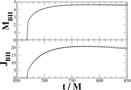
Figure 1: The gravitational mass and angular momentum of the dynamic BH through gravitational collapse for model I. The angular momentum is computed by the approximate Killing vector (solid line), while by dipole moment of the imaginary part of the Weyl scalar $\Psi_{2}$ (dashed line) on the apparent horizon. The gravitational mass is computed by using the first law of BH thermodynamics for both cases.

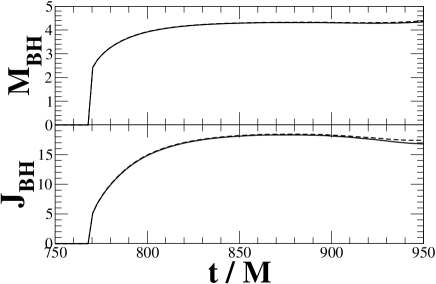
Figure 2: Same as Fig. 1 but for model II.

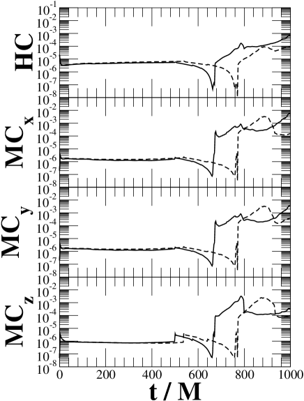
Figure 3: Euclidean norm of the normalised Hamiltonian constraint and the normalised Momentum constraints throughout the evolution for models I (solid line) and II (dashed line).

One of the primary observational missions for detecting gravitational waves in ground-based and space-based interferometers is to investigate a various mass range of BHs and compact objects ((, 1998)). Combining the global network of gravitational wave detectors, we are in these decades able to extract fruitful features of BHs in the frequency band of $10^{-4}{\rm Hz}$ – $10^{3}{\rm Hz}$. Potential sources of high signal to noise events in this frequency range are quasi-periodic waves arising from nonaxisymmetric bars in collapsing relativistic stars and from the inspiral of binary BHs for example (e.g. Ref. ((, 2009))). In addition, a nonspherical collapse of a rotating relativistic star to a BH potentially generates a significant amount of burst waves and quasi-normal ringing waves (e.g. Ref. ((, 2003))). In this paper we trace the collapse of relativistic stars through numerical simulations to investigate some of these possibilities.

Here we relax the condition of uniformly rotating profile in the equilibrium to produce a highly spinning dynamic BH. Differential rotation profile of the star enables us to impose large amount of angular momentum in the system, since it relaxes the restriction to the angular velocity at the equatorial radius, which comes from the limitation of the mass-shedding. According to the above idea, Saijo and Hawke (2009) have succeeded in producing a dynamic BH of spin $J_{\rm final}/M_{\rm final}^{2}\approx 0.98$. Here we focus on the BH configuration in this paper by using multipole moment of the curvatures on the apparent horizon. We try to answer the following questions. Can we extract precisely the mass and angular momentum of a dynamical BH by using multipole moment of the curvatures on the horizon? Can a newly formed BH be represented as a stationary Kerr BH at several dynamical times after the BH formation? Is it useful to use multipole moment of a dynamic BH to extract some properties of a BH, and to find a cause of quasi-periodic gravitational waves after the ringdown, for example? To answer these questions, three spatial dimensional general relativistic hydrodynamics is necessary.

The content of this paper is as follows. In Sec. II, we briefly explain the general relativistic hydrodynamics, especially the numerical tools we use to understand the property of a dynamic BH. In Sec. III, we introduce our findings of a dynamic BH, focusing on its configuration. Section IV is devoted to the summary of this paper. Throughout this paper, we use the geometrized units with $G=c=1$ and adopt Cartesian coordinates $(x,y,z)$ with the coordinate time $t$. Note that Greek index takes $(t,x,y,z)$, while Latin one takes $(x,y,z)$.

II Basic tools in numerical relativity

In this section, we briefly describe three-dimensional relativistic hydrodynamics in full general relativity. We also explain our techniques for investigating outgoing gravitational waves from the sources and a dynamic horizon configuration (see Ref. (Saijo and Hawke, 2009) and references cited therein).

II.1 The gravitational field equations

We define a spatial projection tensor $h^{\mu\nu}\equiv g^{\mu\nu}+n^{\mu}n^{\nu}$, where $g^{\mu\nu}$ is the spacetime metric, $n^{\mu}=(1/\alpha,-\beta^{i}/\alpha)$ the unit normal to the spatial hypersurface, and where $\alpha$ and $\beta^{i}$ are the lapse and shift.

We evolve the spacetime with the 17 spacetime associated variables ($\phi$, $K$, $\tilde{\gamma}_{ij}$, $\tilde{A}_{ij}$, $\tilde{\Gamma}^{i}$), where $e^{\phi}$ is the conformal factor, $K_{ij}$ the extrinsic curvature, $\tilde{\gamma}_{ij}$ the conformally related spatial 3-metric, $\tilde{A}_{ij}$ the conformally related trace-free extrinsic curvature, and $\tilde{\Gamma}^{i}$ the conformal connection function. The evolution equations are

$$\left(\frac{\partial}{\partial t}-{\cal L}_{\beta}\right)\phi = -\frac{1}{6}\alpha K,$$ (1)

$$\left(\frac{\partial}{\partial t}-{\cal L}_{\beta}\right)K = -\gamma^{ij}D_{i}D_{j}\alpha+\alpha\left[\tilde{A}_{ij}\tilde{A}^{ij}+\frac{1}{3}K^{2}+\frac{1}{2}(\rho_{\rm H}+S)\right],$$ (2)

$$\left(\frac{\partial}{\partial t}-{\cal L}_{\beta}\right)\tilde{\gamma}_{ij} = -2\alpha\tilde{A}_{ij},$$ (3)

$$\left(\frac{\partial}{\partial t}-{\cal L}_{\beta}\right)\tilde{A}_{ij} = e^{-4\phi}[-D_{i}D_{j}\alpha+\alpha(R_{ij}-S_{ij})]^{\rm TF}+\alpha(K\tilde{A}_{ij}-2\tilde{A}_{il}\tilde{A}^{l}_{j}),$$ (4)

$$\left(\frac{\partial}{\partial t}-{\cal L}_{\beta}\right)\tilde{\Gamma}^{i} = -2\tilde{A}^{ij}\frac{\partial}{\partial x^{j}}\alpha+2\alpha\left(\tilde{\Gamma}^{i}_{jk}\tilde{A}^{jk}-\frac{2}{3}\tilde{\gamma}^{ij}\frac{\partial}{\partial x^{j}}K-\tilde{\gamma}^{ij}S_{j}+6\tilde{A}^{ij}\frac{\partial}{\partial x^{j}}\phi\right)$$ (5)

$$-\frac{\partial}{\partial x^{j}}\left(\beta^{l}\frac{\partial}{\partial x^{l}}\tilde{\gamma}^{ij}-2\tilde{\gamma}^{m(j}\frac{\partial}{\partial x^{m}}\beta^{i)}+\frac{2}{3}\tilde{\gamma}^{ij}\frac{\partial}{\partial x^{l}}\beta^{l}\right),$$

where ${\cal L}_{\beta}$ denotes the Lie derivative along the shift $\beta^{i}$, $\rho_{\rm H}=T_{\mu\nu}n^{\mu}n^{\nu}$, $S_{i}=T_{\mu\nu}n^{\mu}h^{\nu}_{i}$ and TF the trace-free part of the tensor. This set of equations for solving the Einstein’s field equations numerically is usually called the BSSN formalism. As for gauge conditions, we choose the generalised hyperbolic $K$-driver (Alcubierre et al., 2003) for the lapse, and the generalised hyperbolic $\tilde{\Gamma}$-driver (Baker et al., 2006) for the shift.

II.2 The matter equations

We assume a perfect fluid for describing a relativistic star as

$$T^{\mu\nu}=\rho\left(1+\varepsilon+\frac{P}{\rho}\right)u^{\mu}u^{\nu}+Pg^{\mu\nu},$$ (6)

where $\rho$ is the rest-mass density, $\varepsilon$ the specific internal energy, $P$ the pressure, and $u^{\mu}$ the four-velocity.

Energy momentum conservation $\nabla_{\mu}T^{\mu\nu}=0$ together with a continuity equation, leads to the flux conservative form of the relativistic continuity, the relativistic energy and the relativistic Euler equations as (Banyuls et al., 1997)

$$\frac{1}{\sqrt{-g}}\frac{\partial}{\partial t}(\sqrt{\gamma}{\boldsymbol{\cal U}})+\frac{1}{\sqrt{-g}}\frac{\partial}{\partial x^{i}}(\sqrt{-g}{\boldsymbol{\cal F}}^{i})=\boldsymbol{\cal S}^{i},$$ (7)

where the state vector $\boldsymbol{\cal U}$, the flux vectors $\boldsymbol{\cal F}^{i}$, and the source vectors $\boldsymbol{\cal S}^{i}$ are

$$\boldsymbol{\cal U} = [D,S_{i},\tau]^{T},$$ (8)

$$\boldsymbol{\cal F}^{i} = \left[D\left(v^{i}-\frac{\beta^{i}}{\alpha}\right),S_{j}\left(v^{i}-\frac{\beta^{i}}{\alpha}\right)+P\delta^{i}_{j},\tau\left(v^{i}-\frac{\beta^{i}}{\alpha}\right)+Pv^{i}\right]^{T},$$ (9)

$$\boldsymbol{\cal S}^{i} = \left[0,T^{\mu\nu}\left(\frac{\partial}{\partial x^{\mu}}g_{\nu j}-\Gamma^{\delta}_{\nu\mu}g_{\delta j}\right),\alpha\left(T^{\mu 0}\frac{\partial}{\partial x^{\mu}}\ln\alpha-T^{\mu\nu}\Gamma^{0}_{\nu\mu}\right)\right]^{T},$$ (10)

and $\Gamma^{i}_{~{}jk}$ is a Christoffel symbols. Note that $(\rho,v_{i},\varepsilon)$ are the physical variables of the above equations, and the flux conserved quantities $D$, $S_{i}$, $\tau$ are

$$D = \rho W,$$ (11)

$$W = \alpha u^{t},$$ (12)

$$S_{i} = \rho hW^{2}v_{i},$$ (13)

$$E = \rho hW^{2}-P,$$ (14)

$$\tau = E-D,$$ (15)

where $v_{i}=u_{i}/W$, $h\equiv 1+\varepsilon+P/\rho$ is the specific enthalpy. In the Newtonian limit, the above three physical variables coincide with the rest mass density, the flux density of the rest mass, and the energy of a unit volume of the fluid. In order to solve the set of equations, we have to impose an additional condition among the thermodynamical quantities, namely the equation of state. We adopt a $\Gamma$-law equation of state in the form

$$P=(\Gamma-1)\rho\varepsilon,$$ (16)

where $\Gamma$ is the adiabatic index which we set to $4/3$ in this paper, representing a supermassive star (the pressure is dominated by radiation).

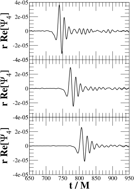
Figure 4: Gravitational waveforms for model I. We monitor the real part of the Weyl scalar $\Psi_{4}$, which represents the plus mode of outgoing waves at null infinity. The observer is located in the $x$-direction of the equatorial plane at $x=65.52M$, $98.29M$, $131.05M$ from the top panel, respectively. Note that the apparent horizon appears in the hypersurface after $t=670.97M$.

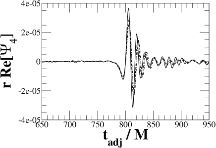
Figure 5: Same as Fig. 4 but adjustment of time shift, plotted in the same panel. Solid, dashed and dash-dotted line denotes the waveform detected in the $x$-direction of the equatorial plane at $x=65.52M$, $98.29M$, $131.05M$. We use the following adjustment of time shift $t_{\rm adj}\equiv t+x_{\rm farthest~{}observer}-x_{\rm obs}$, assuming that gravitational waves propagate with the speed of light in flat spacetime.

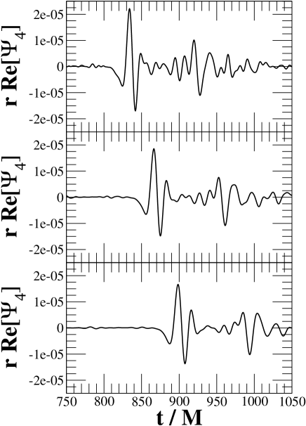
Figure 6: Same as Fig. 4 but for model II. The observer is located in the $x$-direction of the equatorial plane at $x=63.15M$, $94.72M$, $126.30M$ from the top panel, respectively. Note that the apparent horizon appears after $t=770.40M$.

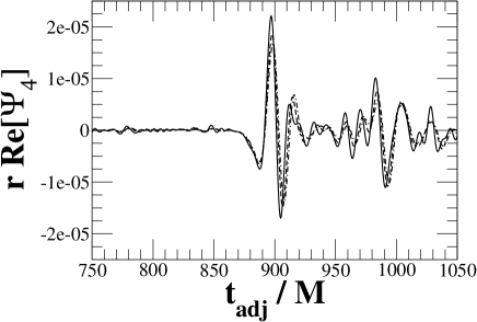
Figure 7: Same as Fig. 6 but adjustment of time shift, plotted in the same panel. Solid, dashed and dash-dotted line denotes the waveform detected in the $x$-direction of the equatorial plane at $x=63.15M$, $94.72M$, $126.30M$. We use the following adjustment of time shift $t_{\rm adj}\equiv t+x_{\rm farthest~{}observer}-x_{\rm obs}$, assuming that gravitational waves propagate with the speed of light in flat spacetime.

II.3 Gravitational waveforms

We monitor the Weyl scalar $\Psi_{4}$ in Newman-Penrose formalism for investigating outgoing gravitational waves as

$$\Psi_{4}=C_{\mu\nu\lambda\sigma}k^{\mu}\bar{m}^{\nu}k^{\lambda}\bar{m}^{\sigma},$$ (17)

where $C_{\mu\nu\lambda\sigma}$ is the Weyl tensor, $k^{\mu}$ the ingoing null vector, $m^{\mu}$ and $\bar{m}^{\mu}$ are the orthogonal spatial-null vectors of the four complex null tetrad ($l^{\mu}$, $k^{\mu}$, $m^{\mu}$, $\bar{m}^{\mu}$). The Weyl scalar $\Psi_{4}$ represents the outgoing gravitational waves at infinity

$$\Psi_{4}=\ddot{h}_{+}-i\ddot{h}_{\times},$$ (18)

where $h_{+}$ and $h_{\times}$ are the two polarisation modes (transverse-traceless condition) of the perturbed metric from flat spacetime in spherical coordinate, and $\dot{q}$ is the time derivative of the quantity $q$. The Weyl scalar $\Psi_{4}$ roughly represents the outgoing gravitational waves, ignoring the radiation scattered back by the curvature when locating the observer far from the source. Therefore we trace the Weyl scalar $\Psi_{4}$ to understand key features of gravitational waves emitted from this system.

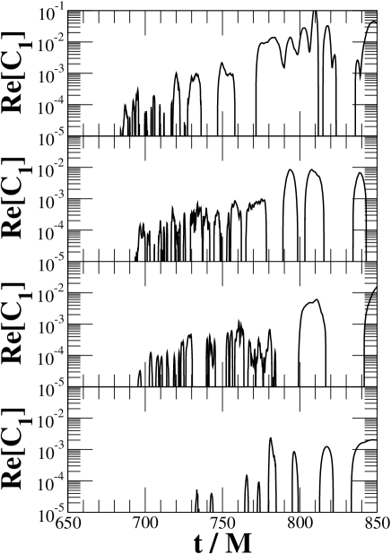
Figure 8: The $m=1$ diagnostics of the rest mass density along the equatorial ring for model I. We measure the diagnostics in the equatorial plane at the radius $r=1.024M$, $2.048M$, $4.095M$, $10.24M$ from the top panel, respectively.

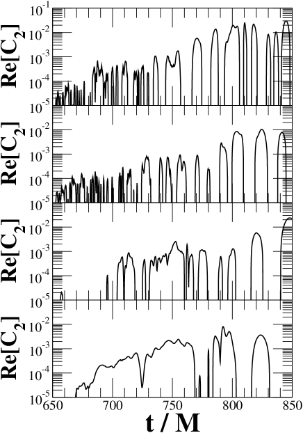
Figure 9: Same as Fig. 8 but for the $m=2$ diagnostics.

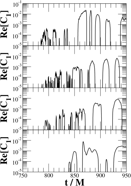
Figure 10: Same as Fig. 8 but for model II. We measure the diagnostics in the equatorial plane at the radius $r=0.987M$, $1.973M$, $3.947M$, $9.867M$ from the top panel, respectively.

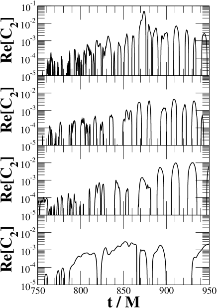
Figure 11: Same as Fig. 10 but for the $m=2$ diagnostics.

II.4 Horizon configuration

Here we introduce a useful idea to diagnose the horizon locally in dynamical spacetime. It is the dynamical horizon defined as the outermost trapped tube which is composed of the apparent horizon in our case (Ashtekar and Krishnan, 2003). First we have to define the angular momentum from the horizon configuration. One way to determine an angular momentum of the dynamic BH is (see e.g. section III.B of Ref. (Schnetter, Krishnan and Beyer, 2006))

$$J_{\rm BH}=-\frac{1}{8\pi}\int_{S_{\rm R}}K_{\mu\nu}R^{\mu}\varphi^{\nu}ds,$$ (19)

where $R^{\mu}$ is the outward directed spacelike normal to the horizon in the spacelike slice, and $\varphi^{a}$ is a rotational vector field on the horizon. This quantity is interpreted as the Komar angular momentum when $\varphi^{a}$ is a rotational Killing vector on the horizon. The code and method used to compute numerically an approximate Killing vector, should it exist, is described in Ref. (Dreyer et al., 2003).

Another way of defining an angular momentum, which is dipole moment of the scalar curvature $\Im\Psi_{2}$, is

$$J_{\rm BH}=-\sqrt{\frac{1}{12\pi}}\frac{A}{4\pi}\int dA\Im\Psi_{2}Y^{l}_{~{}0}(u),$$

where $\Psi_{2}$ is Weyl scalar, $Y^{l}_{~{}m}$ the spherical harmonics, $A$ the area of the horizon and $u$ the polar angle of the horizon configuration. Note that the computations from two different definitions of the angular momentum coincide with each other in an axisymmetric apparent horizon.

The dynamical horizon mass of the hole $M_{\rm BH}$ is computed once we have extracted the angular momentum of the hole by the following relation

$$M_{\rm BH}=\frac{1}{2R_{\rm BH}}\sqrt{R_{\rm BH}+4J_{\rm BH}^{2}}.$$ (20)

Note that $R_{\rm BH}$ is the area radius of the hole.

Axisymmetric isolated horizons are represented by two types of multipole moment of the scalar curvatures on the apparent horizon as (AEPV04, 2004)

$$L_{l} = -\int\Im\Psi_{2}(u)Y^{l}_{~{}0}(u)dA,$$ (21)

$$I_{l} = \int\frac{1}{4}{}^{2}{\cal R}(u)Y^{l}_{~{}0}(u)dA,$$ (22)

where $\Im\Psi_{2}$ is the imaginary part of the Weyl scalar $\Psi_{2}$

$$\Psi_{2}=\frac{1}{2}C_{\mu\nu\lambda\rho}(l^{\mu}n^{\nu}l^{\lambda}n^{\rho}-l^{\mu}n^{\nu}m^{\lambda}\bar{m}^{\rho}),$$

which represents the gravitational monopole at large radius, and ${}^{2}{\cal R}$ the Ricci scalar. The quantities $L_{l}$ and $I_{l}$ correspond to the mass and current $l$-pole moment defined in axisymmetric hole as

$$J_{l} = \sqrt{\frac{4\pi}{2l+1}}\frac{R^{l+1}_{\rm BH}}{4\pi}L_{l},$$ (23)

$$M_{l} = \sqrt{\frac{4\pi}{2l+1}}\frac{M_{\rm BH}R^{l}_{\rm BH}}{2\pi}I_{l}.$$ (24)

This method has two disadvantage when computing multipole moment numerically. One is that the quantities are gauge dependent, and the other is that they become less accurate in the fixed grid of finite differencing when computing higher $l$-pole moment. In order to avoid the above two issues, we use a different method for computing $l$-pole moment of the curvatures by introducing averaged quantities on the trapped surface. We introduce the following “$n$”-pole moment of ${}^{2}{\cal R}$ and $\Im\Psi_{2}$ as (Jasiulek09, 2009)

$$\mu_{n}({}^{2}{\cal R}) = \langle(\langle{}^{2}{\cal R}\rangle-{}^{2}{\cal R})^{n}\rangle,$$ (25)

$$\mu_{n}({\Im\Psi_{2}}) = \langle(\langle{\Im\Psi_{2}}\rangle-{\Im\Psi_{2}})^{n}\rangle,$$ (26)

where the bracket of a physical quantity $\langle Q\rangle$ represents the averaged quantity on the BH horizon

$$\langle Q\rangle = \frac{1}{A}\int Q~{}dA.$$ (27)

The definition of $n$-pole moment is a general extension of defining the variance of quantities. The relations between the quantities $\mu_{n}({}^{2}{\cal R})$ and $\mu_{n}({\Im\Psi_{2}})$, and the mass and current $l$-pole in axisymmetric spacetime are

$$\mu_{n}({}^{2}{\cal R}) = \left\langle\left(1-2\sum_{l=0}^{\infty}I_{l}Y^{l}_{~{}0}(u)\right)^{n}\right\rangle,$$ (28)

$$\mu_{n}({\Im\Psi_{2}}) = \left\langle\left(\sum_{l=0}^{\infty}L_{l}Y^{l}_{~{}0}(u)\right)^{n}\right\rangle.$$ (29)

Therefore $\mu_{n}({}^{2}{\cal R})$ corresponds to the summation of all mass $l$-poles, and $\mu_{n}({\Im\Psi_{2}})$ all current $l$-poles. Since we impose planar symmetry across the equatorial plane, the current odd $l$-poles vanish entirely. The disadvantage of using the quantities $\mu_{n}({}^{2}{\cal R})$ and $\mu_{n}({\Im\Psi_{2}})$, however, is that it is quite difficult to understand their physical situation. Therefore, we introduce the nondimensional quantities for ${}^{2}{\cal R}$ and $\Im\Psi_{2}$ as

$${}^{2}{\cal R} = \frac{8\pi}{A}{}^{2}{\cal\hat{R}},$$ (30)

$${\Im\Psi_{2}} = \frac{2\pi}{A}{\Im\hat{\Psi}_{2}},$$ (31)

from a computational viewpoint.

III Numerical Results

Here we focus on the properties of a dynamic BH through gravitational collapse of a supermassive star. We choose the equilibrium star radially unstable for evolution in order to focus on the BH formation (Saijo and Hawke, 2009).

First we compute the gravitational mass and angular momentum of the hole with two different definitions for the angular momentum in Figs. 1 and 2. One definition for computing the angular momentum is to use the approximated Killing vector, while the other is to use dipole moment of the imaginary part of Weyl scalar $\Psi_{2}$. When the dynamical system is axisymmetric, the computations of the angular momentum by two different definitions coincides with each other. We find a clear agreement of the gravitational mass and angular momentum between two different definitions in Fig. 1 for model I and in Fig. 2 for model II. The results also tell us that our gravitational collapse is nearly the same as an axisymmetric dynamics for both models.

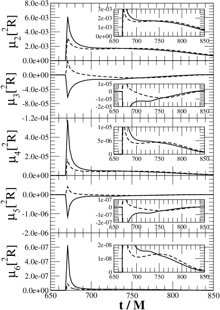
Figure 12: Multipole moment of the Ricci scalar $R$ of the dynamic BH for model I through evolution. Solid line represent the one from our dynamic BH, while dashed line is the one from a Kerr using the gravitational mass and angular momentum of the dynamic BH. We also enlarge the region of quasi-stationary stage at the right part in each panel.

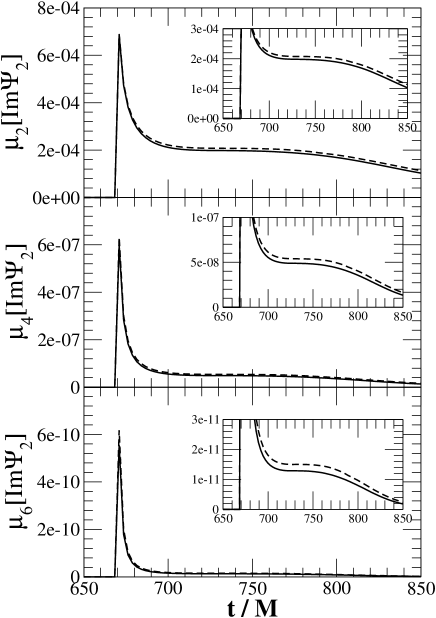
Figure 13: Same as Fig. 12 but for the imaginary part of Weyl scalar $\Psi_{2}$ of the dynamic BH. Note that the odd $l$-pole of $\Im\Psi_{2}$ are exactly zero when we impose planner symmetry across the equator.

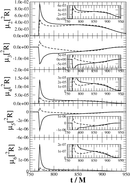
Figure 14: Same as Fig. 12 but for model II.

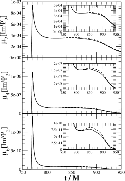
Figure 15: Same as Fig. 13 but for model II.

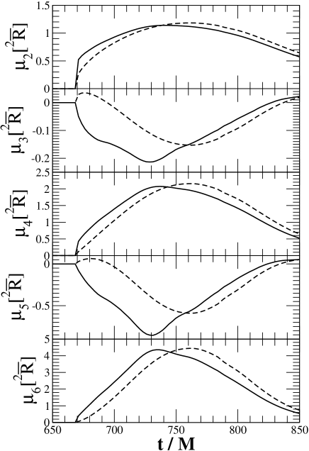
Figure 16: Multipole moment of the Ricci scalar $R$ of the dynamic BH for model I through evolution. Solid line represent the one from our dynamic BH, while dashed line is the one from a Kerr using the gravitational mass and angular momentum of the dynamic BH.

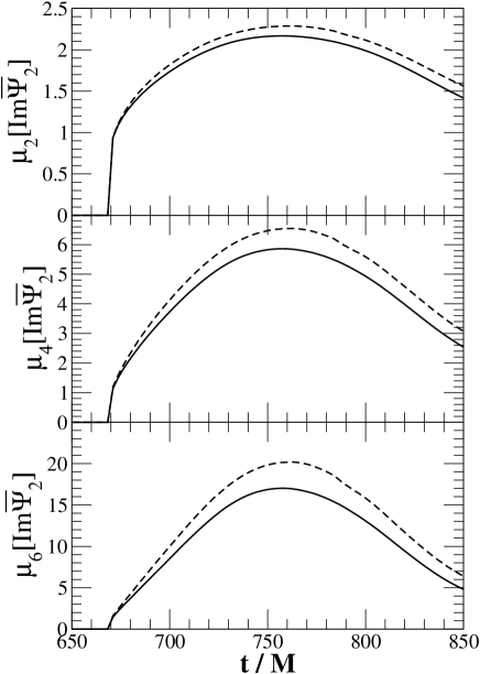
Figure 17: Same as Fig. 16 but for the imaginary part of Weyl scalar $\Psi_{2}$ of the dynamic BH. Note that the odd $l$-pole of $\Im\Psi_{2}$ are exactly zero when we impose planner symmetry across the equator.

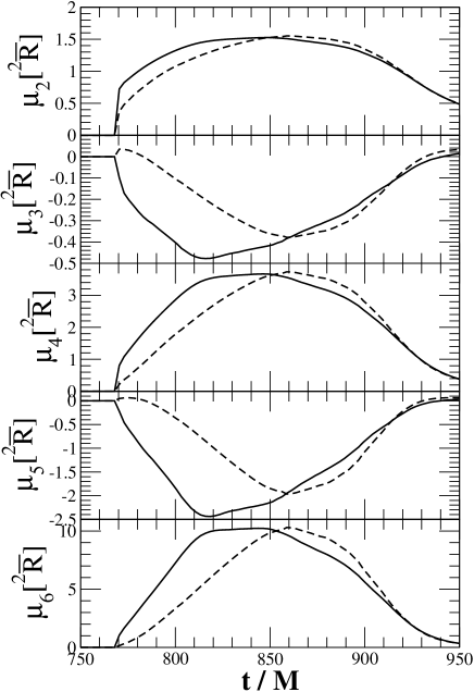
Figure 18: Same as Fig. 16 but for model II.

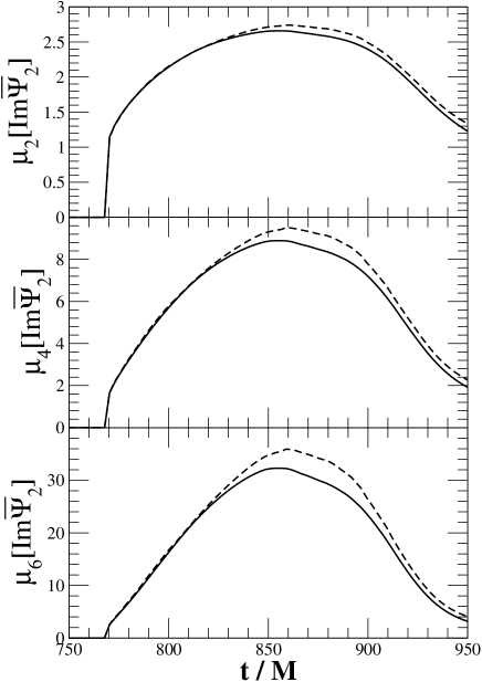
Figure 19: Same as Fig. 17 but for model II.

Next we monitor the Hamiltonian and Momentum constrains through gravitational collapse for monitoring the accuracy of our dynamics in Fig. 3. These checks are necessary because we do not solve these constraints through time integration of the Einstein’s field equations. We diagnose the same quantities as before (Saijo and Hawke, 2009), the Euclidean norm of $HC$ and $MC_{x,y,z}$ of all grid points outside the apparent horizon, through the normalisation of the maximum rest mass density outside the horizon in the same hypersurface. The maximum violations from the constraints of $MC_{x}$ and $MC_{y}$ are less than $1\times 10^{-2}$ for model I and $5\times 10^{-3}$ for model II. These facts tell us that our computational results are very accurate. They are roughly less than around $1\%$ relative error at their worst. However, all the relative violation errors from the constraints for model I increase at the very late time of evolution ($t\approx 900M\sim 1000M$). We therefore stop our time integration at the time around $t\approx 1000M$ to guarantee roughly $1$% relative error or less.

We show gravitational waveforms using the Weyl scalar $\Psi_{4}$ through gravitational collapse in Figs. 4 and 6. The Weyl scalar $\Psi_{4}$ contains both outgoing waves and back-scattered waves by the curvature when we measure the quantity in finite radius from the centre. In order to focus on the outgoing waves, we monitor the waveform at three different locations, and investigate all of them. Since all three locations are considered as radiation zone of gravitational waves from the source, the gravitational field of all three locations is weak, and back-scattered waves only play a secondary role. The outgoing waves propagate towards spatial infinity as time goes on, the features of the outgoing waves can be seen in all three locations with positive time shift. We adjust the time axis of all three waveforms by assuming that gravitational waves propagate with the speed of light, and plot them in the same panel in Figs. 5 and 7. In fact, we use the following relation $t_{\rm adj}\equiv t+x_{\rm farthest~{}observer}-x_{\rm obs}$ to adjust the time. Although there is some difference in the magnitude of the amplitude, the global features look the same. Investigating all three waveforms, we find that the outgoing waves contain three features. The first is that there appears a burst wave as the collapse goes on. The second is that once the BH forms, there is a damping wave which corresponds to a characteristic oscillation of the dynamic BH. The third is that there is a continuous wave after the damping one.

In order to identify the cause of continuous waves after the ringdown, we first investigate the azimuthal modes of the rest mass density. We introduce the following diagnostics at certain radii of a ring in the equatorial plane as

$$C_{m}=\frac{1}{2\pi D_{\rm ring}}\int_{0}^{2\pi}\rho e^{im\varphi}~{}d\varphi,$$

with a normalisation of $D_{\rm ring}(\equiv C_{0})$, a mean density of the ring at certain radii in the equatorial plane. We investigate $m=1$ and $m=2$ diagnostics at 4 different radii for models I and II in Figs. 8 – 11. Although the saturation amplitude for different radii is different for each $m$ diagnostic, we find the following features. The azimuthal diagnostics begin to amplify efficiently after the apparent horizon has appeared in the hypersurface. This feature raises a question as to whether the amplification of the azimuthal diagnostics is directly connected with the configuration of the BH. The saturation amplitude of each $m$ diagnostics is quite similar at the same radius. The saturation amplitude decreases as the radius becomes far from the BH. This feature suggests that the matter which is very close to the BH may play a key role for generating the quasi-periodic waveform after the ringdown.

Next, we investigate the BH configuration to identify a possible cause of the continuous waves. We compute $n$-pole moment of the Ricci scalar ${\cal R}$ and the imaginary part of the Weyl curvature $\Psi_{2}$ on the apparent horizon throughout the evolution. We also compute $n$-pole moment of the same scalar curvatures using the configuration of a Kerr BH. We use the area of the horizon and the nondimensional Kerr parameter $J_{\rm BH}/M_{\rm BH}^{2}$ for computing $n$-pole moment. Then, we compare each $n$-pole in both dimensional definition with the BH area in Figs. 12 – 15, and nondimensional one in Figs. 16 – 19. We find the following two features. The first is that after $t\approx 100M$ time from the formation of the dynamic BH , it is described as a Kerr BH is within a relative error of several percents. If we take the dimension of $n$-poles into account through the area of the BH, $n$-pole of the dynamic BH approaches the one of a Kerr in Figs. 12 and 13 after $t=750M$, and in Figs. 14 and 15 after $t=850M$. Therefore the BH configuration becomes nearly the same as a Kerr after $t\approx 100M$ from the BH formation. This statement suggests that the cause of continuous waves may be related to the matter instability, since the BH configuration is nearly the same as a Kerr. The other is that the odd $n$-pole moment has large deviation from that of a Kerr. This may be accepted fact as the nonaxisymmetric configuration of the rotating BH, as it traces the violent phenomenon at the BH formation. One caution from this feature is that the BH mass and angular momentum are settled down after $t\approx 100M$ from the BH formation time (See Figs. 1 and 2), that the BH is almost regarded as a Kerr. For example, the half-life period of the BH oscillation $\tau(\equiv 1/\Im\omega_{\rm qnm})$ is $13.6M$, since the quasinormal mode frequency of a Kerr BH of $a/M=0.98$ is $M\omega_{\rm qnm}=0.422+0.0735i$ for $l=2$, $m=0$ Leaver (1985). The fact leads to the conclusion that we cannot extract the “stationary” mass and angular momentum of the dynamic BH by quasinormal ringing in principle. Those ringing waves represent vibration of a transient dynamic BH, not a “stationary” one.

IV Conclusions

We investigate the formation of the dynamic BH through gravitational collapse by means of three-dimensional hydrodynamic simulations in general relativity. We particularly focus on the configuration of a dynamic BH and find the following two features.

We investigate two different definitions for the angular momentum of a dynamic BH in order to check the validity of the approximated Killing vector approach. We compare two results from two different definitions for the angular momentum and find that we are able to extract precisely the BH mass and angular momentum even if we use the approximated Killing vector. The fact also indicates that our cases of gravitational collapse are very close to axisymmetric.

We also demonstrate the method to extract $n$-pole moment of the dynamic BH precisely without using the approximated Killing vector. This finding opens a new field of investigating the BH itself by extracting the properties of $n$-poles of the curvatures on the horizon. We compare the configuration of the dynamic BH with that of the Kerr, using multipole moment of the curvatures on the horizon. We find, as a result, that the quasistationary stage of the newly formed BH is approximately described by a Kerr BH. This does not mean, however, that the whole spacetime is approximately represented by a Kerr, since we only investigate the trapped surface of the horizon, just a local structure of the whole spacetime.

Appendix A Multipole moment of the curvatures on the horizon in Kerr spacetime

The 2-surface on the horizon of the Kerr metric in Boyer-Lindquist coordinate is given as

$${}^{2}ds^{2} = \Sigma_{+}d\theta^{2}+\frac{(r_{+}^{2}+a^{2})^{2}}{\Sigma_{+}}\sin^{2}\theta d\varphi^{2}$$ (32)

$$= \eta^{2}[f^{-1}(u)du^{2}+f(u)d\varphi^{2}],$$

where

$$\Sigma_{+} = r_{+}^{2}+a^{2}\cos^{2}\theta,$$ (33)

$$r_{+} = M+\sqrt{M^{2}-a^{2}},$$ (34)

$$\eta = (r_{+}^{2}+a^{2})^{1/2},$$ (35)

$$\beta = a(r_{+}^{2}+a^{2})^{-1/2},$$ (36)

$$u = \cos\theta,$$ (37)

$$f(u) = \frac{1-u^{2}}{1-\beta(1-u^{2})}.$$ (38)

The quantities ${}^{2}{\cal R}$ and $\Im\Psi_{2}$ of the Kerr BH on the horizon are

$${}^{2}{\cal R} = -\frac{8\pi}{A}\frac{d^{2}}{du^{2}}\left[\frac{(1+\hat{c}^{2})(1-u^{2})}{2(1+\hat{c}^{2}u^{2})}\right],$$ (39)

$$\Im\Psi_{2} = \frac{2\pi}{A}\frac{d^{2}}{du^{2}}\left[\frac{u(1+\hat{c}^{2})^{2}}{2\hat{c}(1+\hat{c}^{2}u^{2})}\right],$$ (40)

where

$$\hat{c}=\frac{1-\sqrt{1-\hat{a}^{2}}}{1+\sqrt{1-\hat{a}^{2}}},$$ (41)

and $\hat{a}$ the nondimensional Kerr parameter. In order to compute multipole moment of the horizon only from the nondimensional Kerr parameter and the horizon configuration, we use the nondimensional quantities of the curvatures ${}^{2}\hat{\cal R}$ and $\Im\hat{\Psi}_{2}$.

Then, we can compute multipole moment of the Kerr horizon analytically as

$$\mu_{2}({}^{2}\hat{\cal R}) = \frac{-15-70\hat{c}^{2}+128\hat{c}^{4}+70\hat{c}^{6}+15\hat{c}^{8}}{80(1+\hat{c}^{2})}+\frac{3}{16}(1+\hat{c}^{2})^{4}\frac{\arctan\hat{c}}{\hat{c}},$$ (42)

$$\mu_{3}({}^{2}\hat{\cal R}) = \frac{1125+5745\hat{c}^{2}+10965\hat{c}^{4}-1399\hat{c}^{6}+6999\hat{c}^{8}+6603\hat{c}^{10}+2415\hat{c}^{12}+315\hat{c}^{14}}{2560(1+\hat{c}^{2})^{2}}$$ (43)

$$+\frac{9}{512}(1+\hat{c}^{2})^{4}(-25+14\hat{c}^{2}+7\hat{c}^{4})\frac{\arctan\hat{c}}{\hat{c}},$$

$$\mu_{4}({}^{2}\hat{\cal R}) = \frac{1}{394240(1+\hat{c}^{2})^{3}}(-294525-1755600\hat{c}^{2}-4246935\hat{c}^{4}-5382960\hat{c}^{6}+4201406\hat{c}^{8}+5703728\hat{c}^{10}+6818482\hat{c}^{12}$$ (44)

$$+5017584\hat{c}^{14}+2127279\hat{c}^{16}+480480\hat{c}^{18}+45045\hat{c}^{20})$$

$$+\frac{693}{78848}(1+\hat{c}^{2})^{4}(85-60\hat{c}^{2}+22\hat{c}^{4}+52\hat{c}^{6}+13\hat{c}^{8})\frac{\arctan\hat{c}}{\hat{c}},$$

$$\mu_{5}({}^{2}\hat{\cal R}) = -\frac{1}{7569408(1+\hat{c}^{2})^{4}}(8437275+58760625\hat{c}^{2}+175151130\hat{c}^{4}+296175990\hat{c}^{6}+325931705\hat{c}^{8}-152055293\hat{c}^{10}$$ (45)

$$+104321660\hat{c}^{12}+411065348\hat{c}^{14}+548524189\hat{c}^{16}+426449639\hat{c}^{18}+207094602\hat{c}^{20}+61939878\hat{c}^{22}$$

$$+10465455\hat{c}^{24}+765765\hat{c}^{26})$$

$$-\frac{3465}{7569408}(1+\hat{c}^{2})^{4}(-2435+1710\hat{c}^{2}-1485\hat{c}^{4}-572\hat{c}^{6}+2067\hat{c}^{8}+1326\hat{c}^{10}+221\hat{c}^{12})\frac{\arctan\hat{c}}{\hat{c}},$$

$$\mu_{6}({}^{2}\hat{\cal R}) = \frac{1}{8921808896(1+\hat{c}^{2})^{5}}(-13841202375-111349888650\hat{c}^{2}-396709663350\hat{c}^{4}-835111292730\hat{c}^{6}$$ (46)

$$-1182872163330\hat{c}^{8}-1230909094610\hat{c}^{10}+906857870914\hat{c}^{12}+1101124533086\hat{c}^{14}+1994477265504\hat{c}^{16}$$

$$+3065485548066\hat{c}^{18}+3312605946814\hat{c}^{20}+2475795093330\hat{c}^{22}+1279104290178\hat{c}^{24}+449618015418\hat{c}^{26}$$

$$+102838870134\hat{c}^{28}+13822058250\hat{c}^{30}+829323495\hat{c}^{32})$$

$$+\frac{765765}{8921808896}(1+\hat{c}^{2})^{4}(18075-11240\hat{c}^{2}+15380\hat{c}^{4}-920\hat{c}^{6}-10302\hat{c}^{8}+18216\hat{c}^{10}+23252\hat{c}^{12}+8664\hat{c}^{14}$$

$$+1083\hat{c}^{16})\frac{\arctan\hat{c}}{\hat{c}},$$

$$\mu_{2}(\Im\hat{\Psi}_{2}) = \frac{-15+170\hat{c}^{2}+112\hat{c}^{4}+70\hat{c}^{6}+15\hat{c}^{8}}{80(1+\hat{c}^{2})}+\frac{3}{16}(1+\hat{c}^{2})^{4}\frac{\arctan\hat{c}}{\hat{c}},$$ (47)

$$\mu_{4}(\Im\hat{\Psi}_{2}) = \frac{1}{49280(1+\hat{c}^{2})^{3}}(-3465-36960\hat{c}^{2}+619773\hat{c}^{4}+663168\hat{c}^{6}+1273910\hat{c}^{8}+1306240\hat{c}^{10}+985930\hat{c}^{12}+515328\hat{c}^{14}$$ (48)

$$+178563\hat{c}^{16}+36960\hat{c}^{18}+3465\hat{c}^{20})$$

$$+\frac{693}{9856}(1+\hat{c}^{2})^{8}\frac{\arctan\hat{c}}{\hat{c}},$$

$$\mu_{6}(\Im\hat{\Psi}_{2}) = \frac{1}{8921808896(1+\hat{c}^{2})^{5}}(-271846575-4530776250\hat{c}^{2}-35485039590\hat{c}^{4}+755725266582\hat{c}^{6}+749954442094\hat{c}^{8}$$ (49)

$$+2536970204990\hat{c}^{10}+3859089592210\hat{c}^{12}+5130563563118\hat{c}^{14}+5335972052992\hat{c}^{16}+4426939814290\hat{c}^{18}$$

$$+2910344048750\hat{c}^{20}+1498699974850\hat{c}^{22}+592140524690\hat{c}^{24}+173417402730\hat{c}^{26}+35485039590\hat{c}^{28}$$

$$+4530776250\hat{c}^{30}+271846575\hat{c}^{32})$$

$$+\frac{271846575}{8921808896}(1+\hat{c}^{2})^{12}\frac{\arctan\hat{c}}{\hat{c}}.$$

References

• Rees (2003) M. Rees, in The Future of Theoretical Physics and Cosmology, edited by G. W. Gibbons, E. P. S. Shellard and S. J. Rankin (Cambridge Univ. Press, Cambridge, 2003), 217.
• Miller and Colbert (2004) M. C. Miller and E. J. M. Colbert, Int. J. Mod. Phys.  D 13, 1 (2004).
• Scheel et al. (2009) M. A. Scheel, M. Boyle, T. Chu, L. E. Kidder, K. D. Matthews and H. P. Pfeiffer, Phys. Rev. D79, 024003 (2009).
• Marronetti et al. (2008) P. Marronetti, W. Tichy, B. Brügmann, J. Gonzalez and U. Sperhake, Phys. Rev. D77, 064010 (2008).
• Kesden et al. (2010) M. Kesden, G. Lockhart and E. S. Phinney, Phys. Rev. D82, 124045 (2010).
• Zel’dovich and Novikov (1996) Y. B. Zel’dovich and I. V. Novikov, Stars and Relativity (Dover, New York, 1996), Chap. 11.
• Shibata and Shapiro (2002) M. Shibata and S. L. Shapiro, Astrophys. J. 572, L39 (2002).
• ( (1998)) K. Thorne, in Black Holes and Relativistic Stars, edited by R. M. Wald (Univ. Chicago Press, Chicago), 41.
• ( (2009)) B. S. Sathyaprakash and B. F. Schutz, Living Rev. Relativity 12, 2 (2009).
• ( (2003)) C. L. Fryer and K. C. B. New, Living Rev. Relativity 6, 2 (2003).
• Saijo and Hawke (2009) M. Saijo and I. Hawke, Phys. Rev. D80, 064001 (2009).
• Alcubierre et al. (2003) M. Alcubierre, B. Brügmann, P. Diener, M. Koppitz, D. Pollney, E. Seidel, and R. Takahashi, Phys. Rev. D67, 084023 (2003).
• Baker et al. (2006) J. G. Baker, J. Centrella, D.-I. Choi, M. Koppitz, and J. van Meter, Phys. Rev. Lett. 96, 111102 (2006).
• Banyuls et al. (1997) F. Banyuls, J. A. Font, J. M. Ibàñez, J. M. Martí, and J. A. Miralles, Astrophys. J. 476, 221 (1997).
• Ashtekar and Krishnan (2003) A. Ashtekar and B. Krishnan, Phys. Rev. D68, 104030 (2003).
• Schnetter, Krishnan and Beyer (2006) E. Schnetter, B. Krishnan and F. Beyer, Phys. Rev. D74, 024028 (2006).
• Dreyer et al. (2003) O. Dreyer, B. Krishnan, D. Shoemaker, and E. Schnetter, Phys. Rev. D67, 024018 (2003).
• AEPV04 (2004) A. Ashtekar, J. Engle, T. Pawlowski, C. Van Den Broeck, Class. Quantum Grav. 21, 2549 (2004).
• Jasiulek09 (2009) M. Jasiulek, Class. Quantum Grav. 26, 245008 (2009).
• Leaver (1985) E. W. Leaver, Proc. R. Soc. London A 402, 285 (1985).