The initial conditions of isolated star formation – X. A suggested evolutionary diagram for prestellar cores

R. J. Simpson^1,2, D. Johnstone^3,4, D. Nutter¹, D. Ward-Thompson¹, A. P. Whitworth¹
¹Department of Physics and Astronomy, Cardiff University, Queen’s Buildings, The Parade, Cardiff, CF24 3AA, U.K.
²Oxford Astrophysics, Denys Wilkinson Building, Keble Road, Oxford, OX1 3RH, U.K.
³National Research Council of Canada, Herzberg Institute of Astrophysics, 5071 West Saanich Road, Victoria, BC V9E 2E7, Canada
⁴Department of Physics and Astronomy, University of Victoria, Elliot Building, 3800 Finnerty Road, Victoria, BC V8P 5C2, Canada

(Accepted 20101 May; received 2010 November; in original form 2010 November.)

Abstract

We propose an evolutionary path for prestellar cores on the radius-mass diagram, which is analogous to stellar evolutionary paths on the Hertzsprung-Russell Diagram. Using James Clerk Maxwell Telescope (JCMT) observations of L1688 in the Ophiuchus star-forming complex, we analyse the HCO⁺ (J=4 $\rightarrow$ 3) spectral line profiles of prestellar cores. We find that of the 58 cores observed, 14 show signs of infall in the form of a blue-asymmetric double-peaked line profile. These 14 cores all lie beyond the Jeans mass line for the region on a radius-mass plot. Furthermore another 10 cores showing tentative signs of infall, in their spectral line profile shapes, appear on or just over the Jeans mass line. We therefore propose the manner in which a prestellar core evolves across this diagram. We hypothesise that a core is formed in the low-mass, low-radius region of the plot. It then accretes quasi-statically, increasing in both mass and radius. When it crosses the limit of gravitational instability it begins to collapse, decreasing in radius, towards the region of the diagram where protostellar cores are seen.

keywords:

stars: formation – ISM: dust – infrared: ISM – submillimetre: ISM

^†^†pagerange: 000–000

1 Introduction

Star formation in molecular clouds occurs within pre-protostellar (or prestellar for short) cores, which are gravitationally bound starless cores within the clouds (Ward-Thompson et al., 1994; André et al., 1996; Ward-Thompson et al., 1999; Ward-Thompson, 2002; Ward-Thompson et al., 2007).

Prestellar cores represent the initial conditions for protostellar collapse. Their large-scale physical and chemical properties have been extensively studied. See, for example, Loren et al. (1990); Motte et al. (1998); André et al. (2007) and also DiFrancesco et al. (2007, and references therein). However, the manner in which they evolve is still a matter of some debate (Ward-Thompson et al., 2007, and references therein). In this paper we attempt to address the subject of prestellar core evolution and quantify this evolution with an empirical diagram analogous to the Hertzsprung-Russell Diagram.

In this series of papers we have been investigating the properties of isolated prestellar cores. The term ’isolated’ refers to the idea that these cores are not interacting with each other (André et al., 2007). Paper I (Ward-Thompson et al., 1994) marked the discovery of prestellar cores. Paper II (André et al., 1996) and Paper III (Ward-Thompson et al., 1999), probed 1.3 mm continuum emission from nine prestellar cores with the IRAM telescope and studied their density profiles. Papers IV – VII (Jessop & Ward-Thompson, 2001; Ward-Thompson et al., 2002; Kirk et al., 2005, 2007) used C¹⁸O spectral line, ISO, SCUBA and Spitzer observations respectively to determine the density and temperature profiles of prestellar cores as well as estimating other properties such as their masses and lifetimes. Paper VIII (Simpson et al., 2008) used SCUBA data to measure the masses and radii of prestellar cores in L1688 to demonstrate that the stellar Initial Mass Function (IMF) has its origins in the Core Mass Function (CMF). Paper IX (Nutter et al., 2009) studied prestellar cores in the far-infrared, using Akari observations, and demonstrated that such observations could be dominated by temperature gradients. In this paper we look at infall in prestellar cores.

Table 1: Table of regions showing date of observation, position (in Right Ascension, Declination), size (in arcseconds), position angle of observed HARP maps in this investigation. Right Ascension and Declination of map off positions also shown. All dates of observations are from 2009.

Map	Dates of	R.A.	Declination	Width	Height	PA	Off Pos. R.A.	Off Pos. Declination
	Observations	(2000)	(2000)	(^′′)	(^′′)	(^∘)	(2000)	(2000)
Oph-A	25-26 Apr, 01 May	16^h26^m24.03^s	$-$ 24^∘23^′43.0^′′	690	349	45	16^h25^m52.99^s	$-$ 24^∘25^′23.0^′′
Oph-AN	12,20 Jun	16^h26^m44.07^s	$-$ 24^∘18^′53.7^′′	420	348	50	16^h27^m05.03^s	$-$ 24^∘24^′58.3^′′
Oph-B	15,17,22 May, 02 Jun	16^h27^m22.93^s	$-$ 24^∘28^′17.9^′′	550	348	150	16^h27^m05.03^s	$-$ 24^∘24^′58.3^′′
Oph-C	08,10-11 Jun	16^h26^m55.78^s	$-$ 24^∘34^′16.5^′′	420	348	50	16^h27^m05.03^s	$-$ 24^∘24^′58.3^′′
Oph-E,F	03,04,06-08 Jun	16^h27^m15.76^s	$-$ 24^∘39^′52.4^′′	600	348	40	16^h27^m07.82^s	$-$ 24^∘44^′14.3^′′

The Ophiuchus star-forming region is located at a distance of 139 $\pm$ 6 pc (Mamajek, 2008) and is a site of low-mass star formation (Wilking & Lada, 1983).The region consists of two main clouds, L1688 and L1689, which have extended streamers leading out to distances of around 10 pc (Loren, 1989). Specifically, it is the more massive of the two clouds, L1688, that is studied in this paper, and that is generally known as the Oph main cloud. Very high star formation rates have been measured here with 14-40% of the molecular gas being converted into stars (Vrba, 1977).

The distance to Ophiuchus is a matter of recent debate. Loinard et al. (2008) use radio-emission parallax observations from two young stars in Ophiuchus to calculate a preliminary distance measurement of 120 ${}^{+4.5}_{-4.2}$ pc. Mamajek (2008) and Lombardi et al. (2008) combine extinction maps with parallaxes from Hipparcos and Tycho. These studies find distances of 139 $\pm$ 6 pc and 119 $\pm$ 6 pc respectively. For this analysis we adopt the Mamajek (2008) value because it uses direct parallax measurements of a larger number of objects known to be associated with L1688.

The Oph main cloud has been observed in many wavelengths from the visible to the submillimetre (Montmerle et al., 1983; Wilking et al., 1989; Loren et al., 1990; André et al., 1992; Greene & Young, 1992; Barsony et al., 1997; Motte et al., 1998; Johnstone et al., 2000; Jessop & Ward-Thompson, 2001; Johnstone et al., 2004; Stanke et al., 2006; Enoch et al., 2008; Jørgensen et al., 2008; Padgett et al., 2008; Friesen et al., 2009). Because of this, its properties (e.g. mass, density, temperature, distance) are very well known and it is therefore a good place to study prestellar cores.

Simpson et al. (2008) used SCUBA archive data to produce the deepest 850- $\mu$ m map of L1688. This was used to determine the masses and radii of the prestellar cores in the cloud and to produce a core mass function (CMF). It was shown that the CMF can be fitted to a three-part power law consistent with the form of the stellar initial mass function (IMF). The form of the IMF was hypothesised to be a direct result of the CMF. A similar result was seen for the Orion star-forming region by Nutter & Ward-Thompson (2007).

In this paper we present HCO⁺ (J=4 $\rightarrow$ 3) observations of L1688 taken using the Heterodyne Array Receiver Programme (HARP) instrument on the James Clerk Maxwell Telescope (JCMT). HCO⁺ (J=4 $\rightarrow$ 3) was chosen because it is partially optically thick, which is a requirement for any line to show the characteristic profile for infall described in Section3.2. In addition, HCO⁺ (J=4 $\rightarrow$ 3) can be observed at high spectral and spatial resolution with the JCMT.

2 Observations

HARP is a spectral-imaging receiver for the JCMT, operating at submillimetre wavelengths, in the frequency range 325–375 GHz (Smith et al., 2003, 2008). The HCO⁺ (J=4 $\rightarrow$ 3) line has a rest frequency of 356.7 GHz. HARP works in conjunction with ACSIS – Auto-Correlation Spectral Imaging System (Dent et al., 2000) – a back-end correlator. It provides a spectral resolution of 0.026 kms^-1, and a spatial resolution of 14 arcseconds.

The observations here consist of 40 hours of data taken on multiple nights from April to June 2009. Five fields in L1688 were mapped, and these are outlined in Table 1. The maps were taken in raster position-switch mode. In this mode spectra are taken on the fly, with the telescope scanning in a direction parallel to the sides of the map. At the end of each scan row, the array is displaced by one array-width perpendicular to the scan direction. Another map is created by scanning in a perpendicular direction to the first. These can be combined in a ‘basket-weave’ pattern to create a map with minimal striping due to differences in receptor noise. Separate fixed off-positions were used for each region. These are given in Table 1. These positions were selected as having no 850 $\mu$ m emission (Simpson et al., 2008). They were also checked for HCO⁺ (J=4 $\rightarrow$ 3) emission using a 60-second position-switched ‘stare’ observation.

Refer to caption — Figure 1: Integrated intensity map of HCO⁺ (J=4 $\rightarrow$ 3) toward L1688. Contours at 1.0, 2.0, 3.0, 4.0 and 5.0 Kkms^-1. The scale bar shows integrated intensity in Kkms^-1. All temperatures refer to antenna temperature (T ${}_{A}^{*}$ ).

The data were reduced using the Starlink ¹¹1http://starlink.jach.hawaii.edu/starlink project software KAPPA (Currie et al., 2008, and references therein) and SMURF (Jenness et al., 2008) routines. The data were regridded to a Nyquist-sampled map. It was found that in order to produce the optimal map from the input data, the worst quality data had to be discarded before the map was reconstructed. This was done by measuring the root-mean-square (RMS) noise value of each of the spectra in the input data and masking those with the highest RMS before generating the map. An iterative method was used to determine the optimal RMS value to apply as a mask. In each step of the iteration, the data were masked using a different limiting RMS before being reconstructed into a map using the MAKECUBE routine (Jenness et al., 2008). The RMS in the reconstructed map was then measured. The limiting RMS was varied to produce a reconstructed map with the lowest RMS. This map was taken to be the optimal map.

3 Results

3.1 Maps

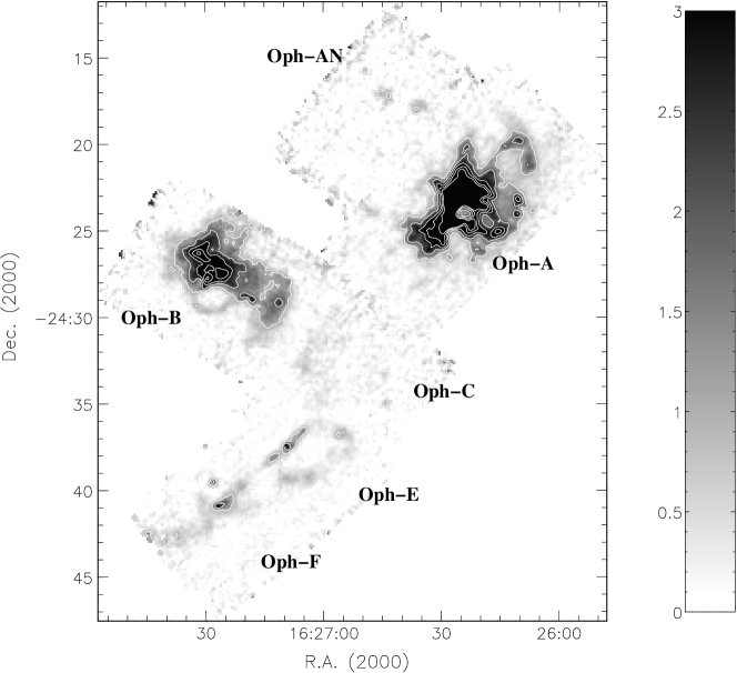
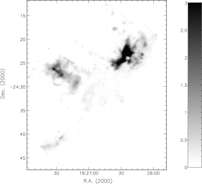
Figure 1 shows the integrated intensity map towards L1688 in HCO⁺ (J=4 $\rightarrow$ 3). A number of sources are seen in the map and the correlation between this integrated HCO⁺ (J=4 $\rightarrow$ 3) map and the submillimetre continuum map shown in Simpson et al. (2008) is consistent, showing that we are tracing the same material. The main regions of the cloud are labelled according to their usual names (Motte et al., 1998).

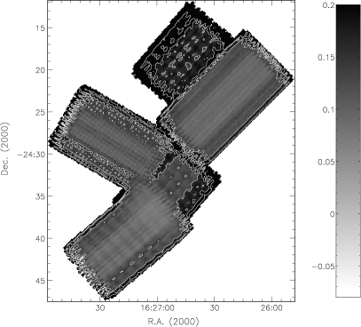
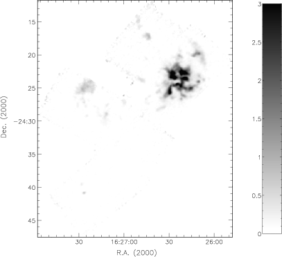
The RMS noise map for the HCO⁺ (J=4 $\rightarrow$ 3) data is shown in Figure 2. Excellent weather conditions gave a very low RMS noise of less than 0.15 K in antenna temperature, T ${}_{A}^{*}$ , for maps of Oph-A, E and F. The noise in Oph-B increases to around 0.2 K toward the edges but most cores are still within the 0.15 K contours. Poorer weather during mapping of Oph-C resulted in a more mixed final map, with some portions mapped to 0.15 K and others to 0.2 K. The lower integration times on Oph-AN mean that the RMS noise level is higher in this region.

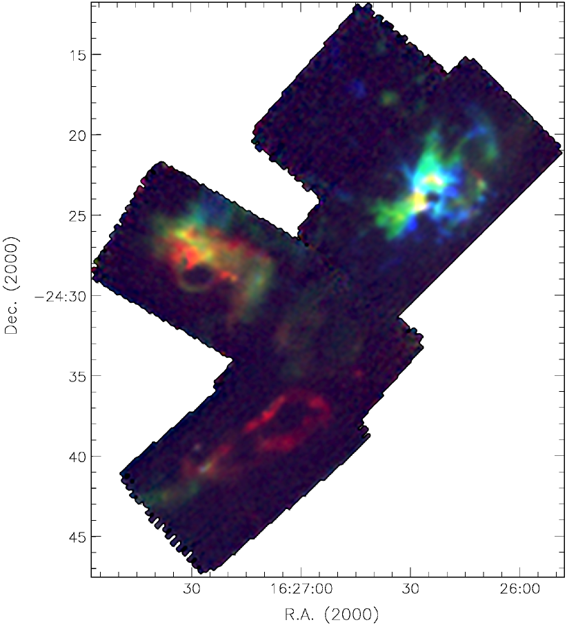
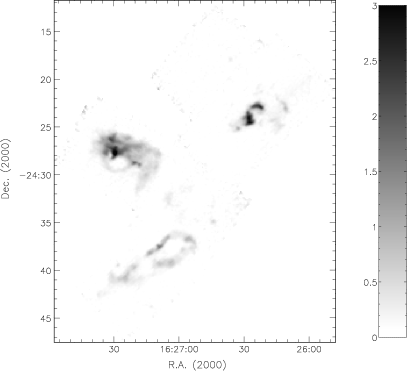
Figure 3 shows the same region as Figure 1 but with a narrower range of velocities. This figure has been split into red (4.0–5.0 kms^-1), green (3.0–4.0 kms^-1) and blue (2.0–3.0 kms^-1) velocity channels, centred around the systemic velocity of L1688 (Loren, 1989). These colour channels were selected to encompass the velocity widths of the observed spectral line profiles. On this version of the map it is clearly seen that Oph-A is moving toward us relative to the rest of L1688. Both Oph-A and B show evidence for HCO⁺ (J=4 $\rightarrow$ 3) outflows and a wide range of velocities are seen in both regions. Oph-E and F appear much redder and are moving away from us relative to the other regions. Figure 4 shows the same data as Figure 3 displayed as three separate images.

Emission is dominated in the integrated intensity map by the bright Oph-A region (e.g. DiFrancesco et al., 2004), containing SM1 (Ward-Thompson et al., 1989) and VLA1623 (André et al., 1993), respectively the prototypical prestellar core and Class 0 object. Both of these sources are highlighted by tightly packed contours in Figure 1. A great deal of structure can be made out in Oph-A. An arch of material is seen traced out just northwest of the brightest part of the region – the northern part of which is moving toward us relative to the southern part. Just south of this arch, a line of sources make up a partial loop that curves around the western edge of the Oph-A region stretching through all the velocity channels.

The Oph-B region (e.g. Friesen et al., 2005) is also very active and a distinct semi-circular loop can be seen on its south side. Both this loop and those in Oph-A have approximate radii of curvature of 0.1pc and have kinematic velocities of the order of 1-2 kms^-1. The northern part of Oph-B is seen moving toward us relative to the rest of the region. This velocity gradient was also visible in ¹³CO (Loren, 1989), DCO⁺ (Loren et al., 1990), and N₂H⁺ (André et al., 2007).

Oph-C appears to be faint in the maps. The weak SCUBA sources measured here by Simpson et al. (2008) seem to have little HCO⁺ (J=4 $\rightarrow$ 3) associated with them. A large, ring-like structure is seen, in the red channel, making up the Oph-E region and this in turn leads into a filament that moves into the green channel as it joins the Oph-F region. Only the northern-most part of the Oph-F region is seen in these maps.

3.2 Spectral Line Profiles

Prestellar cores undergoing collapse, will have excitation temperature profiles that are peaked toward their centre. In addition, we preferentially see material that is closer to us. Material on the near-side of a collapsing core is therefore preferentially seen as less excited than material on the far side. This means that the relatively blue-shifted material is seen to the observer as having a higher excitation temperature. The result is that collapsing cores display an asymmetric spectral line profile, with the peak from material at the blue-shifted end being more prominent than the red-shifted peak. Such a profile shape is referred to as a blue-asymmetric double-peaked profile and can be used as a signpost that collapse is occurring (e.g. Zhou, 1992; Evans, 1999).

We categorise all of the observed prestellar cores based on their HCO⁺ (J=4 $\rightarrow$ 3) spectral line profile shapes: cores with blue-asymmetric double-peaked profiles; cores with faint or only possible blue-asymmetric double-peaked profiles; cores with red-asymmetric double-peaked profiles; cores with single-peaked profiles and cores with unclear profile shapes. Observations of these cores using HCO⁺ (J=4 $\rightarrow$ 3) are not sufficient to determine whether the core is undergoing collapse. Additional measurements of the cores, using an optically thin line tracer, are also required to determine that these double peaks are a spectral, rather than physical effect. For these data, we have included optically thin N₂H⁺ line centres from André et al. (2007). These data were available for the majority of the observed cores and are shown on the 3 $\times$ 3 pixel maps in the Appendix.

Table 2 shows the cores mapped in this study, grouped into regions, along with their HCO⁺ (J=4 $\rightarrow$ 3) profile shapes. The masses and radii for these cores from Simpson et al. (2008) are also shown. Figures 5 – 9 show the HCO⁺ (J=4 $\rightarrow$ 3) spectral line profiles for the same cores, grouped by profile shape.

Table 2: Table showing the Oph cores from Simpson et al. (2008), mapped in this study by HARP. For each core, the radius and mass are given along with the spectral profile shape from our HARP data. Radii are rounded to the nearest 100 AU. Blue-asymmetric and red-asymmetric double-peaked profiles are listed as BAD and RAD respectively. Whether the core was included in the Motte et al. (1998) – MAN98 – is shown for reference, along with an indication of whether the core was seen as a BAD profile in André et al. (2007) – A07.

Core	R.A.	Declination	Radius	Mass	Profile	MAN98	A07
ID	(2000)	(2000)	(AU)	(M_☉)	Shape	Core	BAD
A-MM1	16^h26^m23.00^s	-24^∘23^′34.46^′′	1000	0.09	Single	Y
A-MM2-3	16^h26^m23.80^s	-24^∘24^′09.95^′′	1200	0.16	BAD (Possible)
A-MM4	16^h26^m23.03^s	-24^∘21^′59.81^′′	1000	0.48	BAD	Y
A-MM5	16^h26^m26.66^s	-24^∘22^′28.60^′′	1300	0.82	RAD	Y
A-MM6	16^h26^m28.21^s	-24^∘23^′00.10^′′	1500	2.10	RAD	Y
A-MM7	16^h26^m30.05^s	-24^∘22^′17.93^′′	1400	0.92	BAD	Y
A-MM8	16^h26^m31.80^s	-24^∘24^′50.00^′′	1000	3.18	Single	Y
A-MM11	16^h26^m32.74^s	-24^∘26^′14.40^′′	1600	0.64	Single
A-MM16	16^h26^m36.26^s	-24^∘28^′12.84^′′	1000	0.03	Single
A-MM17	16^h26^m34.77^s	-24^∘28^′08.10^′′	1000	0.03	Single
A-MM18	16^h26^m43.73^s	-24^∘17^′25.74^′′	1700	0.87	Single
A-MM21	16^h26^m31.64^s	-24^∘18^′38.05^′′	1000	0.21	Single
A-MM22	16^h26^m31.45^s	-24^∘18^′52.05^′′	1200	0.11	Unclear
A-MM23	16^h26^m07.89^s	-24^∘20^′30.50^′′	1600	1.50	BAD
A-MM26	16^h26^m15.40^s	-24^∘25^′32.50^′′	1200	0.43	BAD (Possible)
A-MM27	16^h26^m13.85^s	-24^∘25^′25.16^′′	1400	0.34	BAD (Possible)
A-MM30	16^h26^m09.63^s	-24^∘19^′43.25^′′	1500	1.28	Unclear
A2-MM1	16^h26^m11.73^s	-24^∘24^′54.16^′′	1300	0.33	BAD (Possible)	Y
A3-MM1	16^h26^m10.07^s	-24^∘23^′11.00^′′	1200	0.33	Single	Y
A-N	16^h26^m22.74^s	-24^∘20^′00.00^′′	1000	0.21	Single	Y
A-S	16^h26^m42.69^s	-24^∘26^′08.05^′′	1000	0.01	Single
SM1	16^h26^m27.73^s	-24^∘23^′58.17^′′	1800	7.35	RAD	Y
SM1N	16^h26^m27.93^s	-24^∘23^′31.67^′′	1100	2.91	Symmetric	Y
SM2	16^h26^m29.41^s	-24^∘24^′26.69^′′	2200	5.97	RAD	Y	Y
VLA1623	16^h26^m26.74^s	-24^∘24^′30.00^′′	1600	2.93	RAD
B1-MM1	16^h27^m09.32^s	-24^∘27^′43.73^′′	1100	0.02	Unclear	Y
B1-MM2	16^h27^m12.14^s	-24^∘29^′34.42^′′	1200	0.63	BAD	Y
B1-MM3	16^h27^m12.68^s	-24^∘29^′38.67^′′	1300	2.61	BAD	Y
B1-MM4	16^h27^m15.32^s	-24^∘30^′36.82^′′	2000	2.10	Unclear	Y
B1-MM7	16^h27^m18.72^s	-24^∘30^′24.64^′′	1000	0.11	Unclear
B1B2-MM1	16^h27^m12.44^s	-24^∘27^′30.31^′′	1800	0.22	Unclear	Y
B2-MM2	16^h27^m19.97^s	-24^∘27^′23.45^′′	1400	0.88	BAD (Possible)	Y
B2-MM4	16^h27^m24.50^s	-24^∘27^′46.30^′′	1000	0.96	BAD	Y
B2-MM5	16^h27^m24.74^s	-24^∘27^′29.29^′′	1500	1.14	BAD	Y
B2-MM6	16^h27^m25.27^s	-24^∘26^′50.48^′′	2300	1.62	Single	Y
B2-MM7	16^h27^m26.66^s	-24^∘27^′39.72^′′	1700	0.62	BAD (Possible)	Y
B2-MM8	16^h27^m27.96^s	-24^∘27^′06.85^′′	1300	1.63	Unclear	Y
B2-MM9	16^h27^m28.74^s	-24^∘26^′40.65^′′	1400	1.37	BAD	Y
B2-MM13	16^h27^m32.95^s	-24^∘26^′03.16^′′	1500	0.49	BAD (Possible)	Y
B2-MM14	16^h27^m32.53^s	-24^∘26^′27.78^′′	1500	1.26	BAD	Y
B2-MM16	16^h27^m34.49^s	-24^∘26^′11.90^′′	1200	1.31	BAD	Y	Y
C-MM2	16^h26^m59.10^s	-24^∘33^′50.15^′′	1000	1.11	BAD	Y
C-MM3	16^h26^m58.80^s	-24^∘34^′23.40^′′	1900	1.42	Unclear	Y
C-MM5	16^h26^m59.77^s	-24^∘34^′13.87^′′	1100	1.24	BAD	Y	Y
C-MM6	16^h27^m01.58^s	-24^∘34^′44.62^′′	2400	1.05	BAD (Possible)	Y	Y
C-MM8	16^h26^m49.09^s	-24^∘29^′45.15^′′	1000	0.15	Unclear
C-MM9	16^h26^m48.10^s	-24^∘32^′12.50^′′	1100	0.06	Single
C-MM10	16^h27^m02.26^s	-24^∘31^′42.56^′′	1100	0.37	Unclear
C-MM12	16^h26^m59.80^s	-24^∘33^′08.75^′′	1600	0.09	Unclear
C-N	16^h26^m58.11^s	-24^∘31^′46.32^′′	2100	1.60	RAD	Y
E-MM2a	16^h27^m02.89^s	-24^∘38^′46.47^′′	1000	0.12	Single	Y
E-MM2b	16^h27^m02.19^s	-24^∘39^′11.49^′′	1400	0.16	Single	Y
E-MM2d	16^h27^m04.53^s	-24^∘39^′06.42^′′	1000	0.41	BAD	Y	Y
E-MM4	16^h27^m10.67^s	-24^∘39^′25.28^′′	1700	0.31	Unclear	Y	Y
E-MM5	16^h27^m11.67^s	-24^∘37^′57.46^′′	1200	0.28	Single	Y
E-MM8	16^h27^m04.19^s	-24^∘39^′02.59^′′	1200	0.19	BAD (Possible)
F-MM1	16^h27^m21.76^s	-24^∘39^′48.05^′′	1600	1.05	BAD	Y
F-MM2a	16^h27^m24.43^s	-24^∘40^′34.79^′′	2000	1.11	BAD (Possible)	Y

4 Discussion

If we assume that the prestellar cores are at a constant gas-kinetic temperature and are thermally supported (Johnstone et al., 2000, 2001; Kirk et al., 2007), then they will have a radius-mass relationship determined by the external pressure on them. The exact solutions are given by Bonnor-Ebert spheres (Ebert, 1955; Bonnor, 1956). This is in contrast to the cloud at large, where densities are lower and turbulent motions are greater (Kirk et al., 2007).

Assuming an approximately uniform and constant temperature for all the gas in the cloud allows us to calculate the Jeans Mass (Jeans, 1902). Below the Jeans Mass, the internal forces in the core are dominated by thermal pressure. When above the Jeans mass, the core becomes unstable and collapses under its own self-gravity.

Figure 10 shows the cores detected by Simpson et al. (2008) at 850 $\mu$ m with SCUBA, plotted in terms of radius versus mass. Here the radius is defined using the 3 $\sigma$ contour of the signal-to-noise map of the region – see Nutter & Ward-Thompson (2007) and Nutter & Ward-Thompson (2007). The crosses mark the prestellar cores. The cores with associated infrared sources identified by Spitzer, as part of the c2d survey (Enoch et al., 2008), are deemed to be protostellar and are marked with asterisks. We assume that these objects are Class 0 or I protostars (André et al., 1993; Enoch et al., 2009), meaning that they have accreted only part of their final mass. In order to account for the protostellar mass not detected by SCUBA we use a mean IMF mass of 0.6 $M_{\sun}$ (Kroupa, 2002) and thus increase the masses of these objects by 0.3 $M_{\sun}$ . This would be the correction needed if all of the objects lay exactly on the Class 0/I borderline, defined as the point at which a protostar has accreted half of its final main sequence mass (André et al., 1993), and hence is indicative of the correction needed.

We propose the radius versus mass diagram shown in Figure 10 to be the equivalent of an HR diagram for prestellar cores. Cores evolve by accreting mass quasi-statically and maintaining Bonnor-Ebert equilibrium. Upon reaching the Jeans instability, cores collapse to form a protostar, moving downward on this diagram.

Protostellar cores lie beyond the Jeans limit, to the right on the graph, near the resolution limit of the observations. These cores have already accreted material and begun to collapse. Again these cores have been given an additional 0.3 $M_{\sun}$ to account for the undetected mass.

The hypothesis that this diagram illustrates the evolution of prestellar cores can be tested by looking at the position on this diagram occupied by collapsing prestellar cores. If this evolutionary picture is correct, then the blue-asymmetric double-peaked profiles should all lie close to, or beyond the Jeans mass.

Table 2 lists the masses and radii of those starless cores detected by SCUBA, that were also detected in HCO⁺ (J=4 $\rightarrow$ 3) by HARP. Their profile shapes and positions are also given. Figure 11 is the same as Figure 10 except that it shows only the cores listed in Table 2. This time they are plotted according to their spectral line profile shapes. Those cores with blue-asymmetric profiles, indicating collapse, are marked with dark boxes. Cores showing possible infall characteristics are marked with hollow boxes. All other cores are marked as crosses. These cores may simply have the wrong physical conditions to produce a detectable blue-asymmetric profile in HCO⁺ (J=4 $\rightarrow$ 3). Figure 9 shows those cores that display red-asymmetric profiles. These are likely caused by bipolar outflows confusing the signature, especially in the case of VLA1623, which might also interfere with the neighbouring SM1 and SM2. It is noted that this explanation does not necessarily account for the profile of the core C-N, which displays a very thin RAD profile.

In Figures 10 and 11 the two dashed lines marked ‘Low Pressure’ and ‘High Pressure’ show the Bonnor-Ebert relations for external pressures of P/ $k=3\times 10^{6}$ and $12\times 10^{6}~{}\rm{K~{}cm}^{-3}$ respectively (Johnstone et al., 2000; Jørgensen et al., 2008). The solid line in Figure 11 shows a possible evolutionary track, indicating the general direction a core would move through the diagram. This track initially follows a Bonnor-Ebert relation for an external pressure of P/ $k=6\times 10^{6}~{}\rm{K~{}cm}^{-3}$ . We assume a temperature for the cores in Ophiuchus of 10 K (Stamatellos et al., 2007).

The hypothesis that a radius-mass plot can serve as an evolutionary diagram for prestellar cores is supported by these results. In Figure 11, cores showing only weak signs of infall (hollow boxes) appear close to, or beyond, the Jeans mass line compared with those cores exhibiting characteristic infall signatures (solid boxes) which all appear beyond it. 40% of the cores beyond the Jeans mass line show signs of infall; 60% if the possible BAD peaks are included. This supports the conjecture that cores follow an evolutionary track in which they first move diagonally up the diagram, as they accrete material, and then move down it as they cross the Jeans mass limit and collapse.

Using this model, for any given prestellar core on this diagram, an approximate protostellar mass could be derived by following a Bonnor-Ebert track diagonally upward to the Jeans mass line. From that point in the evolution, an efficiency for the collapse of the core needs to be assumed to reach an estimate of the final protostellar mass. If a core continues to accrete whilst collapsing, the gradient of its evolutionary track, after crossing the Jeans mass, will be shallower.

5 Conclusions

We propose that a radius-mass plot can serve as an evolutionary diagram for prestellar cores. Of the 58 prestellar cores observed with HARP, 14 showed signs of infall in the form of a blue-asymmetric double-peaked line profile. These 14 cores all lie beyond the Jeans mass line for the region on such a radius-mass plot. Furthermore those cores showing tentative signs of infall, in their spectral line profile shapes, appear close to, or beyond, the Jeans mass line.

Placing prestellar cores in the context of this evolutionary diagram shows how they can evolve into protostars inside molecular clouds. This analysis could be performed using data for other star-forming clouds, where both submillimetre maps and spectral profile data are available.

Future studies using instruments such as SCUBA-2 and Herschel may be able to probe further to the left on diagram, and see how larger, lower-mass objects – such as CO cores – relate to the gravitationally bound prestellar cores already seen in the continuum. Such objects appear to follow different radius-mass relations to those explored in this study – see Figure 4 of Motte et al. (2001) and discussions by Johnstone et al. (2000, 2001).

Acknowledgments

The authors would to thank Sarah Stickler, Lucy Wilcock and the staff of the JCMT for their help whilst obtaining the data for this study. The JCMT is operated by the Joint Astronomy Centre (JAC) in Hawaii on behalf of the UK Science and Technology Facilities Council (STFC), the Netherlands Organisation for Scientific Research (NWO) and the Canadian National Research Council (NRC). RJS acknowledges STFC studentship support whilst carrying out this work. DN is supported by the Cardiff Astronomy Rolling Grant from STFC.

References

André et al. (2007) André P., Belloche A., Motte F., Peretto N., 2007, Astronomy and Astrophysics, 472, 519
André et al. (1992) André P., Deeney B. D., Phillips R. B., Lestrade J.-F., 1992, The Astrophysical Journal, 401, 667
André et al. (1993) André P., Ward-Thompson D., Barsony M., 1993, The Astrophysical Journal, 406, 122
André et al. (1996) André P., Ward-Thompson D., Motte F., 1996, Astronomy and Astrophysics, 314, 625
Barsony et al. (1997) Barsony M., Kenyon S. J., Lada E. A., Teuben P. J., 1997, The Astrophysical Journal Supplement Series, 112, 109
Bonnor (1956) Bonnor W. B., 1956, Monthly Notices of the Royal Astronomical Society, 116, 351
Currie et al. (2008) Currie M. J., Draper P. W., Berry D. S., Jenness T., Cavanagh B., Economou F., 2008, Astronomical Data Analysis Software and Systems ASP Conference Series, 394, 650
Dent et al. (2000) Dent W. R. F., Duncan W., Ellis M., Harris J., Lightfoot J. F., Wall R., Gibson H., Hills R. E., Richer J., Smith H., Withington S., Burgess T. A., Casorso R. V., Dewdney P. E., Hovey G. J., Redman R. O., Yeung K. K., Force B., Pain I., 2000, Imaging at Radio through Submillimeter Wavelengths, 217, 33
DiFrancesco et al. (2004) DiFrancesco J., André P., Myers P. C., 2004, The Astrophysical Journal, 617, 425
DiFrancesco et al. (2007) DiFrancesco J., Evans N. J., Caselli P., Myers P. C., Shirley Y. L., Aikawa Y., Tafalla M., 2007, Protostars and Planets V, Univ. Arizona Press, Tucson, p. 17
Ebert (1955) Ebert R., 1955, Zeitschrift für Astrophysik, 37, 217
Enoch et al. (2009) Enoch M. L., Evans N. J., Sargent A. I., Glenn J., 2009, The Astrophysical Journal, 692, 973
Enoch et al. (2008) Enoch M. L., Evans N. J., Sargent A. I., Glenn J., Rosolowsky E., Myers P. C., 2008, The Astrophysical Journal, 684, 1240
Evans (1999) Evans N. J., 1999, Annual Review of Astronomy and Astrophysics, 37, 311
Friesen et al. (2009) Friesen R., DiFrancesco J., Shirley Y. L., Myers P. C., 2009, The Astrophysical Journal, 697, 1457
Friesen et al. (2005) Friesen R., Johnstone D., DiFrancesco J., Walsh A., Myers P. C., 2005, Astrochemistry: Recent Successes and Current Challenges, 235, 325P
Greene & Young (1992) Greene T. P., Young E. T., 1992, The Astrophysical Journal, 395, 516
Jeans (1902) Jeans J. H., 1902, Philosophical Transactions of the Royal Society of London. Series A, 199, 1
Jenness et al. (2008) Jenness T., Cavanagh B., Economou F., Berry D. S., 2008, Astronomical Data Analysis Software and Systems ASP Conference Series, 394, 565
Jessop & Ward-Thompson (2001) Jessop N. E., Ward-Thompson D., 2001, Monthly Notices of the Royal Astronomical Society, 323, 1025
Johnstone et al. (2004) Johnstone D., DiFrancesco J., Kirk H., 2004, The Astrophysical Journal, 611, L45
Johnstone et al. (2001) Johnstone D., Fich M., Mitchell G. F., Moriarty-Schieven G., 2001, The Astrophysical Journal, 559, 307
Johnstone et al. (2000) Johnstone D., Wilson C. D., Moriarty-Schieven G., Joncas G., Smith G., Gregersen E. M., Fich M., 2000, The Astrophysical Journal, 545, 327
Jørgensen et al. (2008) Jørgensen J. K., Johnstone D., Kirk H., Myers P. C., Allen L. E., Shirley Y. L., 2008, The Astrophysical Journal, 683, 822
Kirk et al. (2005) Kirk J., Ward-Thompson D., André P., 2005, Monthly Notices of the Royal Astronomical Society, 360, 1506
Kirk et al. (2007) Kirk J., Ward-Thompson D., André P., 2007, Monthly Notices of the Royal Astronomical Society, 375, 843
Kroupa (2002) Kroupa P., 2002, Science, 295, 82
Loinard et al. (2008) Loinard L., Torres R. M., Mioduszewski A. J., Rodríguez L. F., 2008, The Astrophysical Journal, 675, L29
Lombardi et al. (2008) Lombardi M., Lada C. J., Alves J., 2008, Astronomy and Astrophysics, 480, 785
Loren (1989) Loren R. B., 1989, The Astrophysical Journal, 338, 902
Loren et al. (1990) Loren R. B., Wootten A., Wilking B. A., 1990, Astrophysical Journal, 365, 269
Mamajek (2008) Mamajek E. E., 2008, Astronomische Nachrichten, 329, 10
Montmerle et al. (1983) Montmerle T., Koch-Miramond L., Falgarone E., Grindlay J. E., 1983, The Astrophysical Journal, 269, 182
Motte et al. (1998) Motte F., André P., Neri R., 1998, Astronomy and Astrophysics, 336, 150
Motte et al. (2001) Motte F., André P., Ward-Thompson D., Bontemps S., 2001, Astronomy and Astrophysics, 372, L41
Nutter et al. (2009) Nutter D., Stamatellos D., Ward-Thompson D., 2009, Monthly Notices of the Royal Astronomical Society, 396, 1851
Nutter & Ward-Thompson (2007) Nutter D., Ward-Thompson D., 2007, Monthly Notices of the Royal Astronomical Society, 374, 1413
Padgett et al. (2008) Padgett D. L., Rebull L. M., Stapelfeldt K. R., Chapman N. L., Lai S.-P., Mundy L. G., Evans N. J., Brooke T. Y., Cieza L. A., Spiesman W. J., Noriega-Crespo A., McCabe C.-E., Allen L. E., Blake G. A., Harvey P. M., Huard T. L., Koerner D. W., Myers P. C., Sargent A. I., Teuben P. J., van Dishoeck E. F., 2008, The Astrophysical Journal, 672, 1013
Simpson et al. (2008) Simpson R. J., Nutter D., Ward-Thompson D., 2008, Monthly Notices of the Royal Astronomical Society, 391, 205
Smith et al. (2008) Smith H., Buckle J. V., Hills R. E., Bell G., Richer J., Curtis E. I., Withington S., Leech J., Williamson R., Dent W. R. F., Hastings P., Redman R. O., Wooff B., Yeung K. K., Friberg P., 2008, Millimeter and Submillimeter Detectors and Instrumentation for Astronomy IV. Edited by Duncan, 7020, 24
Smith et al. (2003) Smith H., Hills R. E., Withington S., Richer J., Leech J., Williamson R., Gibson H., Dace R., Ananthasubramanian P. G., Barker R. W., Baldwin R., Stevenson H., Doherty P., Molloy D., Quy V., Lush C., 2003, Millimeter and Submillimeter Detectors for Astronomy. Edited by Phillips, 4855, 338
Stamatellos et al. (2007) Stamatellos D., Whitworth A. P., Ward-Thompson D., 2007, Monthly Notices of the Royal Astronomical Society, 379, 1390
Stanke et al. (2006) Stanke T., Smith M. D., Gredel R., Khanzadyan T., 2006, Astronomy and Astrophysics, 447, 609
Vrba (1977) Vrba F. J., 1977, Astronomical Journal, 82, 198
Ward-Thompson (2002) Ward-Thompson D., 2002, Science, 295, 76
Ward-Thompson et al. (2007) Ward-Thompson D., André P., Crutcher R. M., Johnstone D., Onishi T., Wilson C. D., 2007, Protostars and Planets V, Univ. Arizona Press, Tucson, p. 33
Ward-Thompson et al. (2002) Ward-Thompson D., André P., Kirk J., 2002, Monthly Notices of the Royal Astronomical Society, 329, 257
Ward-Thompson et al. (1999) Ward-Thompson D., Motte F., André P., 1999, Monthly Notices of the Royal Astronomical Society, 305, 143
Ward-Thompson et al. (1989) Ward-Thompson D., Robson E. I., Whittet D. C. B., Gordon M. A., Walther D. M., Duncan W., 1989, Monthly Notices of the Royal Astronomical Society, 241, 119
Ward-Thompson et al. (1994) Ward-Thompson D., Scott P. F., Hills R. E., André P., 1994, Monthly Notices of the Royal Astronomical Society, 268, 276
Wilking & Lada (1983) Wilking B. A., Lada C. J., 1983, The Astrophysical Journal, 274, 698
Wilking et al. (1989) Wilking B. A., Lada C. J., Young E. T., 1989, The Astrophysical Journal, 340, 823
Zhou (1992) Zhou S., 1992, The Astrophysical Journal, 394, 204

Appendix A 3x3 pixel HARP maps.

Figures 12 – 69 show the HCO⁺ (J=4 $\rightarrow$ 3) spectral line profiles for the same cores seen in Figures 5 – 9. These plots show the central 3 $\times$ 3 HARP pixels for each core. These plots also show the N₂H⁺ line centres from André et al. (2007) as vertical dashed lines. These data are not available for all cores.