Ticket Entailment is decidable

Abstract

We prove the decidability of the logic $T_{\to}$ of Ticket Entailment. Raised by Anderson and Belnap within the framework of relevance logic, this question is equivalent to the question of the decidability of type inhabitation in simply-typed combinatory logic with the partial basis ${\sf BB^{\prime}IW}$. We solve the equivalent problem of type inhabitation for the restriction of simply-typed lambda-calculus to hereditarily right-maximal terms.

The partial bases built upon the atomic combinators ${\sf B}$, ${\sf B^{\prime}}$, ${\sf C}$, ${\sf I}$, ${\sf K}$, ${\sf W}$ of combinatory logic are well-known for being closely connected with propositional logic. The types of their combinators form the axioms of implicational logic systems that have been studied for well over 70 years [Trigg et al. 1994]. The partial basis ${\sf BB^{\prime}IW}$ corresponds, via the types of its combinators, to the system $T_{\to}$ of Ticket Entailment introduced and motivated in [Anderson and Belnap 1975, Anderson et al. 1990]. The system $T_{\to}$ consists of modus ponens and four axiom schemes that range over the following types for each atomic combinator:

• ${\sf B}$ : $(\chi\to\psi)\to((\phi\to\chi)\to(\phi\to\psi))$

• ${\sf B^{\prime}}$ : $(\phi\to\chi)\to((\chi\to\psi)\to(\phi\to\psi))$

• ${\sf I}$ : $\phi\to\phi$

• ${\sf W}$ : $(\phi\to(\phi\to\chi))\to(\phi\to\chi)$

The type inhabitation problem for ${\sf BB^{\prime}IW}$ is the problem of deciding for a given type whether there exists within this basis a combinator of this type. This problem is equivalent to the problem of deciding whether a given formula can be derived in $T_{\to}$.

Surprisingly, the question of the decidability of $T_{\to}$ has remained unsolved since it was raised in [Anderson and Belnap 1975], although the problem has been thoroughly explored within the framework of relevance logic with proofs of decidability and undecidability for several related systems. For instance the system $R_{\to}$ of Relevant Implication (which corresponds to the basis ${\sf BCIW}$) and the system $E_{\to}$ of Entailment [Anderson and Belnap 1975] are both decidable [Kripke 1959] whereas the extensions $R$, $E$, $T$ of $R_{\to}$, $E_{\to}$, $T_{\to}$ to a larger set of connectives ($\to$, $\wedge$, $\vee$) are undecidable [Urquhart 1984].

In 2004, a partial decidability result for the type inhabitation problem was proposed in [Broda et al. 2004] for a restricted class of formulas – the class of $1$-unary formulas in which every maximal negative subformula is of arity at most 1. Broda, Dams, Finger and Silva e Silva’s approach is based on a translation of the problem into a type inhabitation problem for the hereditary right-maximal (HRM) terms of lambda calculus [Trigg et al. 1994, Bunder 1996, Broda et al. 2004]. The closed HRM-terms form the closure under $\beta$-reduction of all translations of ${\sf BB^{\prime}IW}$-terms, accordingly the type inhabitation problem within the basis ${\sf BB^{\prime}IW}$ is equivalent to the type inhabitation problem for HRM-terms.

We use in this paper the same approach as Broda, Dams, Finger and Silva e Silva’s. We prove that the type inhabitation problem for HRM-terms is decidable, and conclude that the logic $T_{\to}$ is decidable.

Summary

In Section 1, we recall the definition of hereditarily right-maximal terms and the equivalence between the decidability of type inhabitation for ${\sf BB^{\prime}IW}$ and the decidability of type inhabitation for HRM-terms. The principle of our proof is depicted on Figure 1.

In Sections 2 and 3 we provide for each formula $\phi$ a partial characterisation of the inhabitants of $\phi$ in normal form and of minimal size. We show that all those inhabitants belong to two larger sets of terms, the set of compact and locally compact inhabitants of $\phi$.

In Section 4 we show how to associate, with each locally compact inhabitant $M$ of a formula $\phi$, a labelled tree with the same tree structure as $M$. We call this tree the shadow of $M$. We define for shadows the analogue of compactness for terms and prove that the shadow of a compact term is itself compact.

Finally, in Section 5, we prove that for each formula $\phi$ the set of all compact shadows of inhabitants of $\phi$ is a finite set (hence the set of compact inhabitants of $\phi$ is also a finite set), and that this set is effectively computable from $\phi$. The proof appeals to Higman Theorem and Kruskal Theorem – more precisely, to Melliès’ Axiomatic Kruskal Theorem.

The decidability of the type inhabitation problem for HRM-terms and the decidability of $T_{\to}$ follow from this last key result: given an arbitrary formula $\phi$, this formula is inhabited if and only if there exists a compact shadow with the same tree structure as an inhabitant of $\phi$, and our key lemma proves that the existence of such a shadow is decidable.

Figure 1: Principle of the proof of decidability of type inhabitation for HRM-terms.

Preliminaries

The first section of this paper assumes some familiarity with pure and simply-typed lambda-calculus and with the usual notions of $\alpha$-conversion, $\beta$-reduction and $\beta$-normal form [Barendregt 1984, Krivine 1993]. The last three notions are not essential to our discussion, as we later focus exclusively on a particular set of simply-typed terms in $\beta$-normal form. We shall briefly recall the definitions and results used in Section 1.

The set of terms of pure lambda-calculus ($\lambda$-terms) is inductively defined by:

• every variable $x$ is a $\lambda$-term,

• if $M$ is a $\lambda$-term and $x$ is a variable, then $(\lambda xM)$ is a $\lambda$-term,

• if $M,N$ are $\lambda$-terms, then $(MN)$ is a $\lambda$-term.

Terms yielded by the second and third rules are called abstractions and applications respectively. The parentheses surrounding applications and abstractions are often omitted if unambiguous. We let $\lambda x_{1}\dots x_{n}.MN_{1}\dots N_{p}$ abbreviate $(\lambda x_{1}(\dots(\lambda x_{n}(((MN_{1})\dots)N_{p}))\dots))$. For instance, $\lambda xy.x(xy)z$ stands for $(\lambda x(\lambda y((x(xy))z)))$.

The bound variables of $M$ are all $x$ such that $\lambda x$ occurs in $M$. A variable $x$ is free in $M$ if and only:

• $M=x$, or,

• $M=\lambda y.N$, $y\neq x$ and $x$ is free in $N$, or,

• $M=NP$ and $x$ is free in $N$ or free in $P$.

A closed term is a term with no free variables. The raw substitution of $N$ for $x$ in $M$, written $M\langle x\leftarrow N\rangle$, is the term obtained by substituting $N$ for every free occurrence of $x$ in $M$ (every occurrence of $x$ that is not in the scope of a $\lambda x$). We require this substitution to avoid variable capture (for all $y$ free in $N$, no free occurrence of $x$ in $M$ is in the scope of a $\lambda y$):

• if $y=x$, then $y\langle x\leftarrow N\rangle$ is equal to $N$, otherwise it is equal to $y$,

• $(\lambda x.M)\langle x\leftarrow N\rangle=\lambda x.M$,

• if $y\neq x$ and $y$ is free in $N$, then $(\lambda y.M)\langle x\leftarrow N\rangle$ is undefined,

• if $y\neq x$, $y$ is not free in $N$ and $M\langle x\leftarrow N\rangle=M^{\prime}$, then $(\lambda y.M)\langle x\leftarrow N\rangle=\lambda y.M^{\prime}$,

• if $M_{1}\langle x\leftarrow N\rangle=M^{\prime}_{1}$ and $M_{2}\langle x\leftarrow N\rangle=M^{\prime}_{2}$, then $(M_{1}M_{2})\langle x\leftarrow N\rangle=(M^{\prime}_{1}M^{\prime}_{2})$.

The $\alpha$-conversion is defined as the least binary relation $\equiv_{\alpha}$ such that:

• $x\equiv_{\alpha}x$,

• if $M\equiv_{\alpha}M^{\prime}$, $y$ is not free in $M^{\prime}$ and $M^{\prime}\langle x\leftarrow y\rangle=M^{\prime\prime}$, then $(\lambda x.M)\equiv_{\alpha}(\lambda y.M^{\prime\prime})$

• if $M_{1}\equiv_{\alpha}M^{\prime}_{1}$ and $M_{2}\equiv_{\alpha}M^{\prime}_{2}$, then $(M_{1}M_{2})\equiv_{\alpha}(M^{\prime}_{1}M^{\prime}_{2})$.

For instance $\lambda x.y\equiv_{\alpha}\lambda z.y\not\equiv_{\alpha}\lambda y.y$. It is a common practice to consider $\lambda$-terms up to $\alpha$-conversion, however we will not follow this practice in our exposition.

The $\beta$-reduction is the least binary relation $\beta$ satisfying:

• if $M\equiv_{\alpha}(\lambda x.N)P$ and $N\langle x\leftarrow P\rangle=N^{\prime}$, then $M\beta N^{\prime}$.

• if $M\beta M^{\prime}$, then $(\lambda x.M)\beta(\lambda x.M^{\prime})$, $(MN)\beta(M^{\prime}N)$ and $(NM)\beta(NM^{\prime})$.

In the first rule, $x$ is not necessarily free in $N$, so we may have $N=N^{\prime}$ – in particular, free variables may disappear in the process of reduction.

We write $\beta^{*}$ for the reflexive and transitive closure of $\beta$. A term $M$ is in $\beta$-normal form – or $\beta$-normal – if there is no $M^{\prime}$ such that $M\beta M^{\prime}$. A term $M$ is normalising if there is a normal $N$ – called normal form of $M$ – such that $M\beta^{*}N$. It is strongly normalising if there is no infinite sequence $M=M_{0}\beta M_{1}\beta M_{2}\dots$

It is well-known that $\beta$-conversion enjoys the Church-Rosser property: if $M\beta^{*}N$ and $M\beta^{*}N^{\prime}$, then there exist two $\alpha$-convertible $P,P^{\prime}$ such that $N\beta^{*}P$ and $N^{\prime}\beta^{*}P^{\prime}$. As a consequence, if a term is normalising then its normal form is unique up to $\alpha$-conversion.

The judgment “assuming $x_{1},\dots,x_{n}$ are of types $\psi_{1},\dots\psi_{n}$, the term $M$ is of type $\phi$”, written $\{x_{1}:\psi_{1},\dots,x_{n}:\psi_{n}\}\vdash M:\phi$, where $\psi_{1},\dots,\psi_{n},\phi$ are formulas of propositional calculus and $x_{1},\dots,x_{n}$ are distinct variables, is defined by:

• $\Gamma\vdash x:\psi$ for each $x:\psi\in\Gamma$,

• if $\Gamma\cup\{x:\phi\}\vdash M:\psi$, then $\Gamma\vdash\lambda x.M:\phi\to\psi$.

• if $\Gamma\vdash M:\phi\to\psi$ and $\Gamma\vdash N:\phi$, then $\Gamma\vdash(MN):\psi$

The simply-typable terms are all $M$ for which there exist $\Gamma$, $\phi$ such that $\Gamma\vdash M:\phi$. Note that $\Gamma$ contains all variables free in $M$. The following properties are well-known:

1. (Strong normalisation) If $\Gamma\vdash M:\phi$, then $M$ is strongly normalising.

2. (Subject reduction) If $\Gamma\vdash M:\phi$ and $M\beta N$, then $\Gamma\vdash N:\phi$.

1 From ${\sf BB^{\prime}IW}$ to simply-typed lambda-calculus

The aim of this first section is to provide a precise characterisation of simply-typable terms that are typable with inhabited types in ${\sf BB^{\prime}IW}$, so as to transform the problem of type inhabitation in ${\sf BB^{\prime}IW}$ into a type inhabitation problem in lambda-calculus. The types of atomic combinators in ${\sf BB^{\prime}IW}$ are also types for their respective counterparts $\lambda fgx.f(gx)$, $\lambda fgx.g(fx)$, $\lambda x.x$, $\lambda hx.hxx$ in lambda-calculus, hence to each inhabited type $\phi$ in ${\sf BB^{\prime}IW}$ corresponds at least one closed $\lambda$-term of type $\phi$. Moreover, subject reduction and strong normalisation (see above) also ensure the existence of a closed normal $\lambda$-term of type $\phi$. What we lack is a criterion to distinguish amongst all typed normal forms the ones that are reducts of translations of combinators within ${\sf BB^{\prime}IW}$.

The material and the results of this section are not new [Bunder 1996, Broda et al. 2004]. The reader may as well skip the contents of Sections 1.3 and 1.4 entirely, accept Lemma 1.14 then go on with the study of stable parts and blueprints in Section 2.

The definition of hereditarily right-maximal terms is an adaptation of the definition given in [Bunder 1996]. The proof of Lemma 1.6 (subject reduction for HRM-terms) is similar to the proof of Property 2.4, p.375 in [Broda et al. 2004]. The right-to-left implication of Lemma 1.14 can be deduced from Property 2.20, p.390 in [Broda et al. 2004], although our proof method seems to be simpler.

1.1 Lambda-calculus

Let ${\cal X}$ be a countably infinite set of variables $x,y,z\dots$ together with a one-to-one function ${\cal O}$ from ${\cal X}$ to ${\rm Nature}$. For all $x,y$ in ${\cal X}$, we write $x<y$ when ${\cal O}(x)<{\cal O}(y)$. Throughout the sequel, by term we always mean a term of lambda-calculus built over those variables. For each term $M$, we write $\mbox{\sf Free}(M)$ for the strictly increasing sequence of all free variables of $M$.

Terms are not identified modulo $\alpha$-conversion - apart from Section 1, all considered terms will be in normal form, and the Greek letters $\alpha$, $\beta$ will be even used with new meaning at the beginning of Section 2. We adopt however the usual convention according to which two distinct $\lambda$’s may not bound the same variable in a term, and no variable can be simultaneously free and bound in the same term.

1.2 Hereditarily right-maximal terms

Definition 1.1

The set of hereditarily right-maximal (HRM) terms is inductively defined as follows:

1. Each variable $x$ is HRM.

2. If $M$ is HRM and $x$ is the greatest free variable of $M$ then $\lambda x.M$ is HRM.

3. If $M,N$ are HRM, and for each free variable $x$ of $M$ there exists a free variable $y$ of $N$ such that $x\leq y$, then $(MN)$ is HRM.

The second rule ensures that all HRM-terms are $\lambda_{I}$-terms, that is, terms in which every subterm $\lambda x.M$ is such that $x$ is free in $M$. As a consequence the set of free variables of an HRM-term is preserved under $\beta$-reduction. As we shall see below (Lemma 1.6), right-maximality can also be preserved at the cost of appropriate bound variable renamings.

In the third rule, if $N$ is closed then so is $M$. When $M$ and $N$ are non-closed terms, the greatest free variable of $M$ is less than or equal to the greatest free variable of $N$. For instance, if $f<g<x$ and $h<x$, then $\lambda fgx.f(gx)$, $\lambda fgx.g(fx)$, $\lambda x.x$, $\lambda hx.hxx$ are HRM, whereas $\lambda yz.zy$ is not, no matter if $y<z$ or $y>z$.

Definition 1.2

Let $\Omega$ be a function mapping each variable to a formula, in such a way that $\Omega^{-1}(\phi)$ is an infinite set for each $\phi$. We extend this function to the set of all strictly increasing finite sequences of variables, letting $\Omega(x_{1},\dots,x_{n})=(\Omega(x_{1}),\dots,\Omega(x_{n}))$.

Definition 1.3

The judgment $M:\phi$, in words “$M$ is of type $\phi$ w.r.t $\Omega$”, is defined by:

• if $\Omega(x)=\phi$, then $x:\phi$,

• if $x:\chi$, $M:\psi$ and $\lambda x.M$ is HRM, then $\lambda x.M:\chi\to\psi$,

• if $M:\chi\to\psi$, $N:\chi$ and $(MN)$ is HRM, then $(MN):\psi$.

The function $\Omega$ will remain fixed throughout our exposition. Accordingly the type of a term $M$ w.r.t $\Omega$ will be called the type of $M$, without any further reference to the choice of $\Omega$. Note that every typed term is HRM.

Definition 1.4

We write $\Lambda_{\mbox{\rm\scriptsize NF}}$ for the set of all typed terms in $\beta$-normal form. We call $\Lambda_{\mbox{\rm\scriptsize NF}}$-inhabitant of $\phi$ every closed term $M\in\Lambda_{\mbox{\rm\scriptsize NF}}$ of type $\phi$.

The next lemma is the well-known subformula property of simply-typed lambda-calculus:

Lemma 1.5

(Subformula Property) Let $M$ be a $\Lambda_{\mbox{\rm\scriptsize NF}}$-inhabitant of $\phi$. The types of the subterms of $M$ are subformulas of $\phi$.

1.3 Subject reduction of hereditarily right-maximal terms

Lemma 1.6

Suppose there exists a closed $M:\phi$. Then $\phi$ is $\Lambda_{\mbox{\rm\scriptsize NF}}$-inhabited.

Proof 1.7.

(1) We leave to the reader the proof of the fact that for every variable $y$ and for every $N:\phi$, there exists $N^{\prime}\equiv_{\alpha}N$ such that $N^{\prime}:\phi$ and every bound variable of $N^{\prime}$ is strictly greater than $y$.

(2) We prove the following proposition by induction on $P$. Let $P,Q$ be typed HRM-terms. Suppose:

• $x$ and $Q$ are of the same type,

• if $Q$ is closed and $x\in\mbox{\sf Free}(P)$, then $x=\min(\mbox{\sf Free}(P))$

• if $Q$ is not closed, then for all $z\in\mbox{\sf Free}(P)$:

  if $z<x$ then $z\leq\max(\mbox{\sf Free}(Q))$,

  if $x<z$ then $\max(\mbox{\sf Free}(Q))<z$.

• if $Q$ is not closed, then $\max(\mbox{\sf Free}(Q))<z$ for all bound variables $z$ of $P$.

Then $R=P\langle x\leftarrow Q\rangle$ is defined, HRM and of the same type as $P$. The proposition is clear if $P$ is a variable.

Suppose $P=\lambda z.P^{\prime}$. Then $\mbox{\sf Free}(P^{\prime})=\mbox{\sf Free}(P)\cdot(z)$. By induction hypothesis $R^{\prime}=P^{\prime}\langle x\leftarrow Q\rangle$ is defined, HRM and of the same type as $P^{\prime}$. The variable $z$ is still the greatest free variable of $R^{\prime}$ and $z$ is not free in $Q$, hence $R=\lambda z.R^{\prime}$.

Suppose $P=(P_{1}P_{2})$. By induction hypothesis $R_{i}=P_{i}\langle x\leftarrow Q\rangle$ is defined, HRM and of the same type as $P_{i}$ for each $i\in\{1,2\}$. It remains to check that $R=(R_{1}R_{2})$ is HRM. Assume $x$ is free in $P$ and $P_{1}$ is not closed.

Suppose $\max(\mbox{\sf Free}(P_{1}))>x$. Then $\max(\mbox{\sf Free}(P_{1}))=\max(\mbox{\sf Free}(R_{1}))\leq\max(\mbox{\sf Free}(P_{2}))=\max(\mbox{\sf Free}(R_{2}))$.

Suppose $\max(\mbox{\sf Free}(P_{1}))<x$. The term $Q$ cannot be closed, and $\max(\mbox{\sf Free}(P_{1}))=\max(\mbox{\sf Free}(R_{1}))\leq\max(\mbox{\sf Free}(Q))$. We have either $\max(\mbox{\sf Free}(P_{2}))=x$ and $\max(\mbox{\sf Free}(R_{2}))=\max(\mbox{\sf Free}(Q))$, or $\max(\mbox{\sf Free}(P_{2}))>x$ and $\max(\mbox{\sf Free}(P_{2}))=\max(\mbox{\sf Free}(R_{2}))$.

Otherwise $\max(\mbox{\sf Free}(P_{1}))=x$. Suppose $\max(\mbox{\sf Free}(P_{2}))>x$. Then $\max(\mbox{\sf Free}(P_{2}))=\max(\mbox{\sf Free}(R_{2}))$. If $Q$ is closed, then $\mbox{\sf Free}(P_{1})=(x)$ and $R_{1}$ is closed. Otherwise we have $\max(\mbox{\sf Free}(R_{1}))=\max(\mbox{\sf Free}(Q))\leq\max(\mbox{\sf Free}(P_{2}))$. The remaining case is $\max(\mbox{\sf Free}(P_{2}))=x$. If $Q$ is closed then $\mbox{\sf Free}(P_{1})=\mbox{\sf Free}(P_{2})=(x)$ and $R_{1}$, $R_{2}$ are closed. Otherwise $\max(\mbox{\sf Free}(R_{1}))=\max(\mbox{\sf Free}(R_{2})=\max(\mbox{\sf Free}(Q))$.

(3) Assume $N:\phi$ and $N$ is not in normal form. We prove by induction on $N$ the existence of $N^{\prime}:\phi$ such that $N\beta N^{\prime}$. If $N=\lambda x.P$, or if $N=(N_{1}N_{2})$ with $N_{1}$ or $N_{2}$ not in normal form, then the existence of $N^{\prime}$ follows from the induction hypothesis and the fact that $\beta$-reduction preserves the set of free variables of an HRM-term. Otherwise $N=(\lambda x.P)Q$ where for each free variable $z$ of $\lambda x.P$, we have $z<x$ and there exists a free variable $y$ of $Q$ such that $z<y$. By (1) there exists $P^{\prime}\equiv_{\alpha}P$ such that $P^{\prime}:\phi$ and no bound variable of $P^{\prime}$ is less than or equal to a free variable of $Q$. The variable $x$ is the greatest free variable of $P^{\prime}$. By (2), the term $N^{\prime}=P^{\prime}\langle x\leftarrow Q\rangle$ is well-defined, HRM and of the type $\phi$. Moreover $N\beta N^{\prime}$.

(4) We now prove the lemma. The term $M$ is a simply-typable HRM-term. The strong normalisation property implies the existence of a normal form $N$ of $M$. The term $N$ is still a closed term. By (1), there exists $N^{\prime}\equiv_{\alpha}N$ such that $N^{\prime}:\phi$, that is, $\phi$ is $\Lambda_{\mbox{\rm\scriptsize NF}}$-inhabited,

1.4 Equivalence between inhabitation in ${\sf BB^{\prime}IW}$ and $\Lambda_{\mbox{\rm\scriptsize NF}}$-inhabitation

In the next three lemmas by $\phi_{1}\dots\phi_{n}\to\psi$ we mean the formula $(\phi_{1}\to(\dots(\phi_{n}\to\psi)\dots))$ if $n>0$, and otherwise the formula $\psi$. We write $\vdash_{\mbox{\sf\scriptsize BB'IW}\,}\phi$ for the judgment “there exists within the basis ${\sf BB^{\prime}IW}$ a combinator of type $\phi$”.

Lemma 1.8.

If $\vdash_{\mbox{\sf\scriptsize BB'IW}\,}\phi$, then $\phi$ is $\Lambda_{\mbox{\rm\scriptsize NF}}$-inhabited.

Proof 1.9.

If $f<g<x$ and $h<x$, then $\lambda x.x$, $\lambda fgx.f(gx)$, $\lambda fgx.g(fx)$ and $\lambda hx.hxx$ are HRM. For each type $\phi$ of an atomic combinator, the variables $f,g,h,x$ can be chosen so that one of those terms is of type $\phi$. The set of all formulas $\phi$ for which there exists a closed $M$ of type $\phi$ is closed under modus ponens. By Lemma 1.6, every such formula is $\Lambda_{\mbox{\rm\scriptsize NF}}$-inhabited.

Lemma 1.10.

If $\vdash_{\mbox{\sf\scriptsize BB'IW}\,}\chi\to\psi$, then $\vdash_{\mbox{\sf\scriptsize BB'IW}\,}(\phi_{1}\dots\phi_{n}\to\chi)\to(\phi_{1}\dots\phi_{n}\to\psi)$ for all $\phi_{1},\dots,\phi_{n}$.

Proof 1.11.

By induction on $n$, using left-applications of ${\sf B}$.

Lemma 1.12.

Suppose $(i_{1},\dots,i_{n})$, $(j_{1},\dots,j_{m})$, $(k_{1},\dots,k_{p})$ are strictly increasing sequences of integers, $\{k_{1},\dots,k_{p}\}=\{i_{1},\dots,i_{n},j_{1},\dots,j_{m}\}$, $n=0$ or ($n>0$, $m>0$, $i_{n}\leq j_{m}$). If

1. $\vdash_{\mbox{\sf\scriptsize BB'IW}\,}\omega_{i_{1}}\dots\omega_{i_{n}}\to(\chi\to\psi)$,

2. $\vdash_{\mbox{\sf\scriptsize BB'IW}\,}\omega_{j_{1}}\dots\omega_{j_{m}}\to\chi$,

then $\vdash_{\mbox{\sf\scriptsize BB'IW}\,}\omega_{k_{1}}\dots\omega_{k_{p}}\to\psi$.

Proof 1.13.

By induction on $n+m$. The proposition is true if $n=m=0$. Assume $n+m>0$. Then $m>0$.

Suppose $n=0$. Then $(j_{i},\dots,j_{m})=(k_{1},\dots,k_{p})$. We have:
$\begin{array}[]{ll}(\mbox{\rm i})&\vdash_{\mbox{\sf\scriptsize BB'IW}\,}(\chi\to\psi)\to((\omega_{j_{m}}\to\chi)\to(\omega_{j_{m}}\to\psi))\\ (\mbox{\rm ii})&\vdash_{\mbox{\sf\scriptsize BB'IW}\,}(\omega_{j_{m}}\to\chi)\to(\omega_{j_{m}}\to\psi)\end{array}$
where: (i) is a type for ${\sf B}$; (ii) follows from (i), (1) and modus ponens. If $m=1$ then $\vdash_{\mbox{\sf\scriptsize BB'IW}\,}\omega_{j_{1}}\to\psi$ follows from (ii), (2) and modus ponens. Otherwise $\vdash_{\mbox{\sf\scriptsize BB'IW}\,}\omega_{j_{1}}\dots\omega_{j_{m}}\to\psi$ follows from (ii), (2) and the induction hypothesis.

We now assume $n>0$. Suppose $m>1$ and $i_{n}\leq j_{m-1}$. Then
$\begin{array}[]{ll}(\mbox{\rm iii})&\vdash_{\mbox{\sf\scriptsize BB'IW}\,}(\chi\to\psi)\to((\omega_{j_{m}}\to\chi)\to(\omega_{j_{m}}\to\psi))\\ (\mbox{\rm iv})&\vdash_{\mbox{\sf\scriptsize BB'IW}\,}(\omega_{i_{1}}\dots\omega_{i_{n}}\to(\chi\to\psi))\to(\omega_{i_{1}}\dots\omega_{i_{n}}\to((\omega_{j_{m}}\to\chi)\to(\omega_{j_{m}}\to\psi)))\\ (\mbox{\rm v})&\vdash_{\mbox{\sf\scriptsize BB'IW}\,}\omega_{i_{1}}\dots\omega_{i_{n}}\to((\omega_{j_{m}}\to\chi)\to(\omega_{j_{m}}\to\psi))\end{array}$
where: (iii) is a type for ${\sf B}$; (iv) follows from (iii) and Lemma 1.10; (v) follows from (iv), (1) and modus ponens. We have $k_{p}=j_{m}$ and $\{k_{1},\dots,k_{p-1}\}=\{i_{1},\dots,i_{n},j_{1},\dots,j_{m-1}\}$. Since $i_{n}\leq j_{m-1}$, we have $\vdash_{\mbox{\sf\scriptsize BB'IW}\,}\omega_{k_{1}}\dots\omega_{k_{p-1}}\to(\omega_{j_{m}}\to\psi)$ by (v), (2) and the induction hypothesis.

Suppose $m=1$ or ($m>1$ and $i_{n}>j_{m-1}$). Then
$\begin{array}[]{ll}(\mbox{\rm vi})&\vdash_{\mbox{\sf\scriptsize BB'IW}\,}(\omega_{j_{m}}\to\chi)\to((\chi\to\psi)\to(\omega_{j_{m}}\to\psi))\\ (\mbox{\rm vii})&\vdash_{\mbox{\sf\scriptsize BB'IW}\,}(\omega_{j_{1}}\dots\omega_{j_{m}}\to\chi)\to(\omega_{j_{1}}\dots\omega_{j_{m-1}}\to((\chi\to\psi)\to(\omega_{j_{m}}\to\psi)))\\ (\mbox{\rm viii})&\vdash_{\mbox{\sf\scriptsize BB'IW}\,}\omega_{j_{1}}\dots\omega_{j_{m-1}}\to((\chi\to\psi)\to(\omega_{j_{m}}\to\psi))\\ (\mbox{\rm ix})&\vdash_{\mbox{\sf\scriptsize BB'IW}\,}\omega_{n_{1}}\dots\omega_{n_{q}}\to(\omega_{j_{m}}\to\psi)\end{array}$
where: (vi) is a type for ${\sf B^{\prime}}$; (vii) follows from (vi) and Lemma 1.10; (viii) follows from (vii), (2) and modus ponens; $\{n_{1},\dots,n_{q}\}=\{j_{1},\dots,j_{m-1},i_{1},\dots,i_{n}\}$; (ix) follows from (viii), (1) and the induction hypothesis. If $j_{m}>i_{n}$, then $(n_{1},\dots,n_{q},j_{m})=(k_{1},\dots,k_{p})$. Otherwise $j_{m}=i_{n}$, $n_{q}=i_{n}$, $(n_{1},\dots n_{q})=(k_{1},\dots,k_{p})$ and
$\begin{array}[]{ll}(\mbox{\rm x})&\vdash_{\mbox{\sf\scriptsize BB'IW}\,}\omega_{k_{1}}\dots\omega_{k_{p-1}}\to(\omega_{i_{n}}\to(\omega_{i_{n}}\to\psi))\\ (\mbox{\rm xi})&\vdash_{\mbox{\sf\scriptsize BB'IW}\,}(\omega_{i_{n}}\to(\omega_{i_{n}}\to\psi))\to(\omega_{i_{n}}\to\psi)\\ (\mbox{\rm xii})&\vdash_{\mbox{\sf\scriptsize BB'IW}\,}(\omega_{k_{1}}\dots\omega_{k_{p-1}}\to(\omega_{i_{n}}\to(\omega_{i_{n}}\to\psi)))\to(\omega_{k_{1}}\dots\omega_{k_{p-1}}\to(\omega_{i_{n}}\to\psi))\\ (\mbox{\rm xiii})&\vdash_{\mbox{\sf\scriptsize BB'IW}\,}\omega_{k_{1}}\dots\omega_{k_{p-1}}\to(\omega_{i_{n}}\to\psi)\end{array}$
where: (x) is (ix); (xi) is a type for ${\sf W}$; (xii) follows from (xi) and Lemma 1.10; (xiii) follows from (x), (xii) and modus ponens; (xiii) is $\vdash_{\mbox{\sf\scriptsize BB'IW}\,}\omega_{k_{1}}\dots\omega_{k_{p}}\to\psi$.

Lemma 1.14.

For every formula $\phi$, we have $\vdash_{\mbox{\sf\scriptsize BB'IW}\,}\phi$ if and only if $\phi$ is $\Lambda_{\mbox{\rm\scriptsize NF}}$-inhabited.

Proof 1.15.

The left to right implication is Lemma 1.8. Using Lemma 1.12 when $M$ is an application, an immediate induction on $M$ shows that if $M:\psi$, $\mbox{\sf Free}(M)=(x_{1},\dots,x_{n})$ and $x_{1}:\chi_{1},\dots,x_{n}:\chi_{n}$, then $\vdash_{\mbox{\sf\scriptsize BB'IW}\,}\chi_{1}\dots\chi_{n}\to\psi$

2 Stable parts and blueprints

The last lemma showed that the decidability of type inhabitation for ${\sf BB^{\prime}IW}$ is equivalent to the decidability of $\Lambda_{\mbox{\rm\scriptsize NF}}$-inhabitation. The sequel is devoted to the elaboration of a decision algorithm for the latter problem.

The problem we shall examine throughout Sections 2 and 3 is the following: if an inhabitant is not of minimal size, is there any way to transform it (with the help of grafts and/or another compression of some sort) into a smaller inhabitant of the same type? This question is not easy because we are dealing with a lambda-calculus restricted with strong structural constraints (righ-maximality). There are however simple situations in which an inhabitant is obviously not of minimal size.

Consider a $\Lambda_{\mbox{\rm\scriptsize NF}}$-inhabitant $M$ and two subterms $N,P$ of $M$ such that $P$ is a strict subterm of $N$. Suppose:

• $N,P$ are applications of the same type or abstractions of the same type.

• $\mbox{\sf Free}(N)=X=(x_{1},\dots,x_{n})$,

• $\mbox{\sf Free}(P)=Y=(y^{1}_{0},\dots,y^{1}_{p_{1}},\dots,y^{n}_{0},\dots,y^{n}_{p_{n}})$

• $\Omega(X)=(\chi_{1},\dots,\chi_{n})$,

• $\Omega(Y)=(\chi^{1}_{0},\dots,\chi^{1}_{p_{1}},\dots,\chi^{n}_{0},\dots,\chi^{n}_{p_{n}})$,

• $\chi^{i}_{j}=\chi_{i}$ for each $i,j$.

Then $M$ is not of minimal size. Indeed we can rename the free variables of $P$ (letting $\rho(y^{i}_{j})=x_{i}$) so as to obtain a term $P^{\prime}$ of the same size as $P$, of the same type and the same free variables as $N$. The subterm $N$ of $M$ can be replaced with $P^{\prime}$ in $M$. The resulting term is a $\Lambda_{\mbox{\rm\scriptsize NF}}$-inhabitant of the same type but of strictly smaller size.

This simple property is far from being enough to characterise the minimal inhabitants of a formula: there are indeed formulas with inhabitants of abitrary size in which this situation never occurs. What we need is a more flexible way to reduce the size of non-minimal inhabitants. In particular, we need a better understanding of our available freedom of action if we are to rename the free variables of a term – possibly occurrence by occurrence – and if we want to ensure that right-maximality is preserved. This section is devoted to the proof of two key lemmas that delimit this freedom.

• In Sections 2.1, 2.2 and 2.2 we show how to build from any term $M\in\Lambda_{\mbox{\rm\scriptsize NF}}$ a partial tree labelled with formulas. This partial tree is called the blueprint of $M$. This blueprint can be seen as a synthesized version of $M$ that contains all and only the information required to determine whether a (non-uniform) renaming of the free variables of $M$ will preserve hereditarily right-maximality.

• In Sections 2.4 and 2.5 we introduce a rewriting relation on blueprints that allows one to “extract” sequences of formulas from a blueprint.

• In section 2.6 we prove our two key lemmas. Lemma 2.17 clarifies the link between the blueprints of $M$ and $\lambda x.M$ (provided both are in $\Lambda_{\mbox{\rm\scriptsize NF}}$). This lemma proves in particular that the sequence of the types of the free variables of $M$ (that is, $\Omega(\mbox{\sf Free}(M))$) can always be extracted from its blueprint. Lemma 2.19 shows that for every sequence of formulas $\overline{\phi}$ that can be extracted from the blueprint of $M$, there exists a (non-uniform) renaming of the free variables of $M$ that will produce a term $N$ of the same type and with the same blueprint as $M$, and such that $\Omega(\mbox{\sf Free}(N))=\overline{\phi}$.

As a continuation of our first example, let us examine the consequences of this last result. Consider again a $\Lambda_{\mbox{\rm\scriptsize NF}}$-inhabitant $M$ and two subterms $N,P$ of $M$ such that $P$ is a strict subterm of $N$ and $N,P$ are applications of the same type or abstractions of the same type. Suppose:

• the sequence $\Omega(\mbox{\sf Free}(N))$ can be extracted from the blueprint of $P$.

This situation is a generalization of the preceding one (in our first example $\Omega(X)$ could also be extracted from the blueprint of $P$, see Definition 2.11). The term $M$ is still not of minimal size. Indeed, we may use the second key lemma to prove the existence of (non-uniform) renaming of the free variables of $P$ that will produce a term $P^{\prime}$ of the same type as $P$ such that $\mbox{\sf Free}(P^{\prime})=\mbox{\sf Free}(N)$. The term $N$ can be replaced with $P^{\prime}$ in $M$.

2.1 Partial trees and trees

Definition 2.1.

Let $({{\mathbb{A}}\,},\leq)$ be the set of all finite sequences over the set ${\rm Nature}_{+}$ of natural numbers, ordered by prefix ordering. Elements of ${{\mathbb{A}}\,}$ are called addresses. We call partial tree every function $\pi$ whose domain is a set of addresses. For each partial tree $\pi$ and for each address $a$, we let ${\pi}_{|a}$ denote the partial tree $c\mapsto\pi(a\cdot c)$ of domain $\{c\,|\,a\cdot c\in{\mbox{\rm dom}}(\pi)\}$.

Definition 2.2.

For all partial trees $\pi,\pi^{\prime}$ and for every address $a$, we let $\pi[a\leftarrow\pi^{\prime}]$ denote the partial tree $\pi^{\prime\prime}$ such that ${\pi^{\prime\prime}}_{|a}=\pi^{\prime}$ and $\pi^{\prime\prime}(b)=\pi(b)$ for all $b\in{\mbox{\rm dom}}(\pi)$ such that $a\not\leq b$.

Definition 2.3.

A tree domain is a set $A\subseteq{{\mathbb{A}}\,}$ such that for all $a\in A$: every prefix of $a$ is in $A$; for every integer $i>0$, if $a\cdot(i)\in A$, then $a\cdot(j)\in A$ for each $j\in\{1,\dots,i-1\}$. A tree domain $A$ is finitely branching if and only if for each $a\in A$, there exists an $i>0$ such that $a\cdot(i)$ is undefined. We call tree every function whose domain is a tree domain.

In the sequel terms will be freely identified with trees. We identify: $x$ with the tree mapping $\varepsilon$ to $x$; $\lambda x.M$ with the tree $\tau$ mapping $\varepsilon$ to $\lambda x$ and such that ${\tau}_{|(1)}$ is the tree of $M$; $(M_{1}M_{2})$ with the tree $\tau$ mapping $\varepsilon$ to $@$ and such that ${\tau}_{|(i)}$ is the tree of $M_{i}$ for each $i\in\{1,2\}$.

2.2 Blueprints

Definition 2.4.

Let ${\mathfrak{S}}$ be the signature consisting of all formulas and all symbols of the form $@_{\phi}$ where $\phi$ is a formula. Each formula is considered as a symbol of null arity. Each $@_{\phi}$ is of arity 2.

We call blueprint every finite partial tree $\alpha:A\to{\mathfrak{S}}$ satisfying the following condition: for each $a\in A$, if $\alpha(a)=@_{\phi}$, then ${\alpha}_{|a\cdot(1)}$ and ${\alpha}_{|a\cdot(2)}$ are of non-empty domains. A rooted blueprint is a blueprint $\alpha$ such that $\varepsilon\in{\mbox{\rm dom}}(\alpha)$.

For each ${\cal S}\subseteq{\mathfrak{S}}$, we call ${\cal S}$-blueprint every blueprint whose image is a subset of ${\cal S}$. We write ${{\mathbb{B}}\hskip 0.86108pt}({\cal S})$ for the set of all ${\cal S}$-blueprints, and ${{\mathbb{B}}\hskip 0.86108pt}_{\varepsilon}({\cal S})$ for the set of all rooted ${\cal S}$-blueprints.

Definition 2.5.

For every blueprint $\alpha$ and every address $a$, the relative depth of $a$ in $\alpha$ is the number of $b\in{\mbox{\rm dom}}(\alpha)$ such that $b<a$. The relative depth of $\alpha$ is defined as $0$ if $\alpha$ is of empty domain, the maximal relative depth of an address in $\alpha$ otherwise.

In the sequel the following notations will be used to denote blueprints (see Figure 2):

• $\emptyset_{\,{\mathbb{B}}\,}$ denotes the blueprint of empty domain.

• we abbreviate $\varepsilon\mapsto\phi$ as $\phi$.

• $@_{\phi}(\alpha_{1},\alpha_{2})$ denotes the (rooted) blueprint $\alpha$ such that $\alpha(\varepsilon)=\phi$, ${\alpha}_{|(1)}=\alpha_{1}$, ${\alpha}_{|(2)}=~{}\alpha_{1}$.

• for every sequence $\overline{a}=(a_{1},\dots,a_{k})$ of pairwise incomparable addresses, $\ast_{\overline{a}}(\alpha_{1},\dots,\alpha_{k})$ denotes the blueprint $\alpha$ of minimal domain such that ${\alpha}_{|a_{i}}=\alpha_{i}$ for each $i\in[1,\dots,k]$.

• we let $\ast(\alpha_{1},\dots,\alpha_{k})$ denote the blueprint $\ast_{\overline{a}}(\alpha_{1},\dots,\alpha_{k})$ such that $\overline{a}=((1),\dots,(k))$.

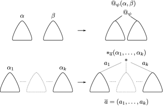
Figure 2: Construction of blueprints, with the notations of Section 2.2. In the upper diagram, the blueprints $\alpha$ and $\beta$ must be non-empty. Although $\alpha_{1},\dots,\alpha_{k}$ are displayed from left to right, the sequence $(a_{1},\dots,a_{k})$ needs not to be lexicographically ordered.

For each blueprint $\alpha$, the choice of $\overline{a},\alpha_{1},\dots,\alpha_{k}$ such that $\alpha=\ast_{\overline{a}}(\alpha_{1},\dots,\alpha_{k})$ is obviously not unique. The sequence $(\alpha_{1},\dots,\alpha_{k})$ may contain an arbitrary number of empty blueprints, hence the sequence $\overline{a}$ may be of arbitrary length. Also, $\alpha$ can be roooted (if $k=1$, $a_{1}=\varepsilon$ and $\alpha_{1}$ is rooted) or empty (if $k=0$ or $\alpha_{1}=\dots=\alpha_{k}=\emptyset_{\,{\mathbb{B}}\,}$). Those ambiguities will not be difficult to deal with, but they will require a few precautions in our proofs and definitions by induction on blueprints.

2.3 Blueprint of a term

Definition 2.6.

For all $M\in\Lambda_{\mbox{\rm\scriptsize NF}}$, the stable part of $M$ is the set of all $a\in{\mbox{\rm dom}}(M)$ such that $\mbox{\sf Free}({M}_{|a})\subseteq\mbox{\sf Free}(M)$ and ${M}_{|a}$ is a variable or an application.

It is easy to check that our conventions (no variable is simultaneously free and bound in a term) ensure that the stable part of a term does not depend on the choice of variable names. Since $M$ is in normal form, $M$ is of empty stable part if and only if it is closed.

Definition 2.7.

For all $M\in\Lambda_{\mbox{\rm\scriptsize NF}}$, we call blueprint of $M$ the function $\alpha$ mapping each $a$ in the stable part of $M$ to:

• $\psi$    if ${M}_{|a}$ is a variable of type $\psi$,

• $@_{\psi}$ if ${M}_{|a}$ is an application of type $\psi$.

We let $M\Vdash\alpha$ denote the judgment “$M$ is of blueprint $\alpha$” (Figure 3).

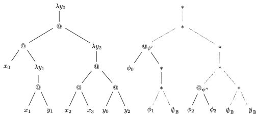
Figure 3: An element of $\Lambda_{\mbox{\rm\scriptsize NF}}$ with its blueprint ($x_{0}<x_{1}<y_{1}$, $x_{2}<x_{3}<y_{0}<y_{2}$, $x_{1}<y_{0}<y_{2}$).

If $M=(M_{1}M_{2})\in\Lambda_{\mbox{\rm\scriptsize NF}}$, $M:\phi$, $M_{1}\Vdash\alpha_{1}$, $M_{2}\Vdash\alpha_{2}$, then each $\alpha_{i}$ is of non-empty domain and $(M_{1}M_{2})\Vdash@_{\phi}(\alpha_{1},\alpha_{2})$ – in other words the so-called blueprint of $M$ is indeed a blueprint, provided so are the blueprints of $M_{1}$, $M_{2}$. When $M=\lambda x.M_{1}$ the blueprint of $M$ is of the form $*(\alpha)$ – the relation between $\alpha$ and the blueprint of $M_{1}$ in that case will be clarified by Lemma 2.17.

Lemma 2.8.

For all $M\in\Lambda_{\mbox{\rm\scriptsize NF}}$ and forall $a\cdot b\in{\mbox{\rm dom}}(M)$:

1. If $\mbox{\sf Free}({M}_{|a\cdot b})\subseteq\mbox{\sf Free}(M)$ then $\mbox{\sf Free}({M}_{|a\cdot b})\subseteq\mbox{\sf Free}({M}_{|a})$.

2. If ${M}_{|a}\Vdash\alpha$ and ${M}_{|a\cdot b}\Vdash\beta$, then ${\alpha}_{|b}=\beta$.

Proof 2.9.

The first proposition is a consequence of our bound variable convention (see Section 1.1): if $\mbox{\sf Free}(M)=X$, $\mbox{\sf Free}({M}_{|a})=X^{\prime}\cup Y$ where $X^{\prime}\subseteq X$ and $X$, $Y$ are disjoint, then every element of $\mbox{\sf Free}({M}_{|a\cdot b})$ in $X$ is also an element of $X^{\prime}$. Thus if $a\cdot b$ is in the stable part of $M$, then $b$ is also in the stable part of ${M}_{|a}$. The second proposition is equivalent to the first.

2.4 Extraction of the formulas of a blueprint

Definition 2.10.

The judgment “$\beta$ is the blueprint obtained by extracting the formula $\phi$ at the address $a$ in the blueprint $\alpha$”, written $\alpha\rhd^{a}_{\phi}\beta$, is inductively defined by:

1. $\phi\rhd^{\varepsilon}_{\phi}\emptyset_{\,{\mathbb{B}}\,}$,

2. if $\alpha\rhd^{a}_{\phi}\beta$, then $@_{\psi}(\gamma,\alpha)\rhd^{(2)\cdot a}_{\phi}*(\gamma,\beta)$

3. if $\alpha\rhd^{a}_{\phi}\beta$, then $*_{(b,c_{1},\dots,c_{k})}(\alpha,\gamma_{1},\dots,\gamma_{k})\rhd^{b\cdot a}_{\phi}*_{(b,c_{1},\dots,c_{k})}(\beta,\gamma_{1},\dots,\gamma_{n})$.

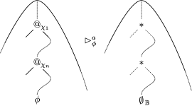
Figure 4: Principle of blueprint reduction.

In (2) we assume of course that $\alpha$ and $\gamma$ are non-empty. In (3) we assume $b\neq\varepsilon$ in order to avoid circularity.

For instance (Figure 5):

Figure 5: Full reductions of $@_{\psi}(\chi\to\psi,@_{\chi}(\phi\to\chi,\phi))$ to $\emptyset_{\,{\mathbb{B}}\,}$.

• $\begin{array}[t]{lll}@_{\psi}(\chi\to\psi,@_{\chi}(\phi\to\chi,\phi))&\rhd^{(2,2)}_{\phi}&*(\chi\to\psi,*(\phi\to\chi,\emptyset_{\,{\mathbb{B}}\,}))\vspace{1ex}\\ &\rhd^{(2,1)}_{\phi\to\chi}&*(\chi\to\psi,*(\emptyset_{\,{\mathbb{B}}\,},\emptyset_{\,{\mathbb{B}}\,}))\vspace{1ex}\\ &\rhd^{(1)}_{\chi\to\psi}&*(\emptyset_{\,{\mathbb{B}}\,},*(\emptyset_{\,{\mathbb{B}}\,},\emptyset_{\,{\mathbb{B}}\,}))=\emptyset_{\,{\mathbb{B}}\,}\vspace{1ex}\end{array}$

• $\begin{array}[t]{lll}@_{\psi}(\chi\to\psi,@_{\chi}(\phi\to\chi,\phi))&\rhd^{(2,2)}_{\phi}&*(\chi\to\psi,*(\phi\to\chi,\emptyset_{\,{\mathbb{B}}\,}))\vspace{1ex}\\ &\rhd^{(1)}_{\chi\to\psi}&*(\emptyset_{\,{\mathbb{B}}\,},*(\phi\to\chi,\emptyset_{\,{\mathbb{B}}\,}))\vspace{1ex}\\ &\rhd^{(2,1)}_{\phi\to\chi}&*(\emptyset_{\,{\mathbb{B}}\,},*(\emptyset_{\,{\mathbb{B}}\,},\emptyset_{\,{\mathbb{B}}\,}))=\emptyset_{\,{\mathbb{B}}\,}\end{array}$

When $\alpha\rhd^{a}_{\phi}\beta$, the blueprint $\beta$ can be seen as $\alpha$ in which the formula $\phi$ at $a$ is erased together with all $@$’s in the path to $a$. At each $@$ this path must follow the right branch of $@$. The constraints on the construction of blueprints imply the existence of at least one such path in every non-empty blueprint, even if it is not the blueprint of a term.

2.5 Sets of extractible sequences

Definition 2.11.

For each formula $\phi$, let $\rhd_{\phi}$ be the relation defined by: $\alpha\rhd_{\phi}\beta$ if and only if there exists $a$ such that $\alpha\rhd^{a}_{\phi}\beta$. We write $\rhd^{+}_{\phi}$ for the transitive closure of $\rhd_{\phi}$. For each $\alpha$, we write ${{\mathbb{F}}\,}(\alpha)$ for the set of all sequences $(\phi_{1},\dots,\phi_{n})$ such that $\alpha\rhd^{+}_{\phi_{n}}\dots\rhd^{+}_{\phi_{1}}\emptyset_{\,{\mathbb{B}}\,}$.

The set ${{\mathbb{F}}\,}(\alpha)$ is what we called “set of extractible sequences of $\alpha$” in the introduction of Section 2. Note that ${{\mathbb{F}}\,}(\emptyset_{\,{\mathbb{B}}\,})=\{\varepsilon\}$. If $\alpha\neq\emptyset_{\,{\mathbb{B}}\,}$, then all elements of ${{\mathbb{F}}\,}(\alpha)$ are non-empty sequences. Note also that each $\rhd$-reduction strictly decreases the cardinality of the domain of a blueprint, therefore ${{\mathbb{F}}\,}(\alpha)$ is a finite set for all $\alpha$. We now introduce the notion of shuffle which will allow us to characterise ${{\mathbb{F}}\,}(\alpha)$ depending on the structure of $\alpha$.

Definition 2.12.

A contraction of a sequence $F$ is either the sequence $F$ or a sequence $G\cdot(f)\cdot H$ where $G\cdot(f)\cdot(f)\cdot H$ is a contraction of $F$.

Definition 2.13.

For all finite sequences $F_{1},\dots,F_{n}$ we call shuffle of $(F_{1},\dots,F_{n})$ every sequence $F^{1}_{1}\cdot\dots\cdot F^{1}_{n}\cdot\dots\cdot F^{p}_{1}\cdot\dots\cdot F^{p}_{n}$ such that $F^{1}_{i}\cdot\dots\cdot F^{p}_{i}=F_{i}$ for each $i$. For each tuple of sets of finite sequences $({\cal F}_{1},\dots,{\cal F}_{n})$ we write $\circledast({\cal F}_{1},\dots,{\cal F}_{n})$ for the closure under contraction of the set of shuffles of elements of ${\cal F}_{1}\times\dots\times{\cal F}_{n}$.

Definition 2.14.

Given two non-empty finite sequences $F_{1},F_{2}$, we call right-shuffle of $(F_{1},F_{2})$ every sequence $F^{1}_{1}\cdot F^{1}_{2}\cdot\dots\cdot F^{p}_{1}\cdot F^{p}_{2}$ such that $F^{1}_{i}\cdot\dots F^{p}_{i}=F_{i}$ for each $i$ and $F^{p}_{2}\neq\varepsilon$. For each pair of sets of non-empty finite sequences $({\cal F}_{1},{\cal F}_{2})$ we write $\circledcirc({\cal F}_{1},{\cal F}_{2})$ for the closure under contraction of the set of right-shuffles of elements ${\cal F}_{1}\times{\cal F}_{2}$.

Figure 6: Shuffling of two sequences. The chunks of $F$ and $G$ need not to be of the same size – some of them can be empty. Every contraction of the resulting sequence belongs to $\circledast(F,G)$. Each contraction belongs also to $\circledcirc(F,G)$ when $F,G$ are non-empty and the last chunk $G^{p}$ of $G$ is non-empty.

The principle of (right-)shuffling is depicted on Figure 6. The following properties follow from our definitions and will be used without reference:

1. If $\alpha=\emptyset_{\,{\mathbb{B}}\,}$, then ${{\mathbb{F}}\,}(\alpha)=\{\varepsilon\}$.

2. If $\alpha=\phi$, then ${{\mathbb{F}}\,}(\alpha)=\{(\phi)\}$.

3. If $\alpha=*_{\overline{a}}(\alpha_{1},\dots,\alpha_{k})$, then ${{\mathbb{F}}\,}(\alpha)=\circledast({{\mathbb{F}}\,}(\alpha_{1}),\dots,{{\mathbb{F}}\,}(\alpha_{k}))$.

4. If $\alpha=@_{\phi}(\alpha_{1},\alpha_{2})$, then ${{\mathbb{F}}\,}(\alpha)=\circledcirc({{\mathbb{F}}\,}(\alpha_{1}),{{\mathbb{F}}\,}(\alpha_{2}))$.

2.6 Abstraction vs. extraction

Lemma 2.15.

Suppose $\{a_{1},\dots,a_{p}\}=\{b_{1},\dots,b_{p}\}$, and:

• $\alpha\rhd^{a_{1}}_{\chi}\dots\rhd^{a_{p}}_{\chi}\beta$,

• $\alpha\rhd^{b_{1}}_{\chi}\dots\rhd^{b_{p}}_{\chi}\beta^{\prime}$.

Then $\beta=\beta^{\prime}$.

Proof 2.16.

By an easy induction on $\alpha$.

Recall that for every strictly increasing sequence of variables $X=(x_{1},\dots,x_{n})$, we write $\Omega(X)$ for the sequence of the types of $x_{1},\dots,x_{n}$. We now clarify the link between the blueprint $\alpha$ of a term $M$ and the one of $\lambda x.M$.

The next lemma shows in particular that if $M,\lambda x.M\in\Lambda_{\mbox{\rm\scriptsize NF}}$, then $M$ and $\lambda x.M$ are of blueprints $\alpha$ and $\beta$ if and only if there exist $a_{0},\dots,a_{p}$ such that $\{a_{0},\dots,a_{p}\}=\{a\,|\,{M}_{|a}~{}=~{}x\}$, $\alpha\rhd^{a_{0}}_{\chi}\dots\rhd^{a_{p}}_{\chi}\alpha^{\prime}$ and $\beta=*(\alpha^{\prime})$ (Figure 7).

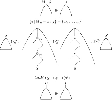
Figure 7: How the blueprint of $M$ evolves into the blueprint of $\lambda x.M$

Lemma 2.17.

Suppose $M\in\Lambda_{\mbox{\rm\scriptsize NF}}$ is of blueprint $\alpha$, with $\mbox{\sf Free}(M)=(x_{1},\dots,x_{n})$ and $\Omega(x_{1},\dots,x_{n})=(\chi_{1},\dots,\chi_{n})$. For each $i\in[0,\dots,n]$:

• let $\alpha_{i}$ be the restriction of $\alpha$ to ${\mbox{\rm dom}}(\alpha)\cap\{a\,|\,\mbox{\sf Free}({M}_{|a})\subseteq\{x_{1},\dots,x_{i}\}\}$.

• let $\beta_{i}$ be the blueprint of $\lambda x_{i+1}\dots x_{n}.M$,

Then:

1. For each $i\in[0,\dots,n]$ we have ${\mbox{\rm dom}}(\beta_{i})=\{1^{n-1}\cdot a\,|\,a\in{\mbox{\rm dom}}(\alpha_{i})\}$ and ${\beta_{i}}_{|1^{n-i}}=\alpha_{i}$.

2. For each $i\in\,\,]0,\dots,n]$:

   1. there exist $a^{i}_{0},\dots,a^{i}_{p_{i}}$ such that $\{a^{i}_{0},\dots,a^{i}_{p_{i}}\}=\{a\,|\,{M}_{|a}=x_{i}\}$

      and $\alpha_{i}\rhd^{a^{i}_{0}}_{\chi_{i}}\dots\rhd^{a^{i}_{p_{i}}}_{\chi_{i}}\alpha_{i-1}$,

   2. if $\{b_{0},\dots,b_{p_{i}}\}=\{a\,|\,{M}_{|a}=x_{i}\}$ and $\alpha_{i}\rhd^{b_{0}}_{\chi_{i}}\dots\rhd^{b_{p_{i}}}_{\chi_{i}}\alpha^{\prime}$ then $\alpha^{\prime}=\alpha_{i-1}$.

3. We have $(\chi_{1},\dots,\chi_{n})\in{{\mathbb{F}}\,}(\alpha)$.

Proof 2.18.

Property (1) follows immediately from the definition of a blueprint. Since $\alpha_{n}~{}=~{}\alpha$ and $\alpha_{0}=\emptyset_{\,{\mathbb{B}}\,}$, Property (3) follows from Property (2.a). Property (2.b) follows from Property (2.a) and Lemma 2.15. As to prove (2.a) we introduce the following notations.

For each $N\in\Lambda_{\mbox{\rm\scriptsize NF}}$, we let $\rho_{N}$ be the least partial function satisfying the following conditions: for every blueprint $\gamma$, we have $\rho_{N}(\varepsilon,\gamma)=\gamma$; for every finite sequence of variables $Y$ and for every blueprint $\gamma$, if $\rho_{N}(Y,\gamma)=\delta$, $\{b\,|\,{N}_{|b}=y\}=\{b_{0},\dots,b_{m}\}$ and $\delta\rhd^{b_{0}}_{\chi}\dots\rhd^{b_{m}}_{\chi}\delta^{\prime}$, then $\rho_{M}((y)\cdot Y,\gamma)=\delta^{\prime}$. By Lemma 2.15, if $\{b\,|\,{N}_{|b}=y\}=\{b_{0},\dots,b_{m}\}=\{c_{0},\dots,c_{m}\}$, $\delta\rhd^{b_{0}}_{\chi}\dots\rhd^{b_{m}}_{\chi}\delta^{\prime}$ and $\delta\rhd^{c_{0}}_{\chi}\dots\rhd^{c_{m}}_{\chi}\delta^{\prime\prime}$, then $\delta^{\prime}=\delta^{\prime\prime}$, thus $\rho_{N}$ is indeed a function. For each finite sequence of variables $Y^{\prime}$ and for each blueprint $\gamma$, we let $\mu_{N}(Y^{\prime},\gamma)$ be the restriction of $\gamma$ to ${\mbox{\rm dom}}(\gamma)\cap\{b\,|\,\mbox{\sf Free}({N}_{|b})\subseteq Y^{\prime}\}$.

We shall prove by induction on $M$ that for all pairs $(X,X^{\prime})$ such that $\mbox{\sf Free}(M)=X\cdot X^{\prime}$, we have $\mu_{M}(X,\alpha)=\rho_{N}(X^{\prime},\alpha)$ – in particular for all $i>0$ we have

$$\begin{array}[]{ll}\alpha_{i-1}&=\mu_{M}((x_{1},\dots,x_{i-1}),\alpha)\\ &=\rho_{M}((x_{i},\dots,x_{n}),\alpha)\\ &=\rho_{M}((x_{i}),\rho_{M}((x_{i+1}\dots,x_{n}),\alpha))\\ &=\rho_{M}((x_{i}),\mu_{M}((x_{1}\dots,x_{i}),\alpha))\\ &=\rho_{M}((x_{i}),\alpha_{i})\end{array}$$

thus (2.a) holds. The case $X^{\prime}=\varepsilon$ is immediate, hence we may as well assume that $X^{\prime}$ is a non-empty suffix of $\mbox{\sf Free}(M)$. The case of $M$ equal to a variable follows immediately from our definitions.

Suppose $M=(M_{1}M_{2})$, $M_{1}\Vdash\gamma_{1}$ and $M_{2}\Vdash\gamma_{2}$. There exist $X_{1},X_{2},X^{\prime}_{1},X^{\prime}_{2}$ such that: $X_{1}\cup X_{2}=X$; $X^{\prime}_{1}\cup X^{\prime}_{2}=X^{\prime}$; $\mbox{\sf Free}(M_{j})=X_{j}\cdot X^{\prime}_{j}$ for each $j\in\{1,2\}$. We have $\alpha=@_{\psi}(\gamma_{1},\gamma_{2})$ where $\psi$ is the type of $M$, and $\mu_{M}(X,\alpha)=\ast(\mu_{M_{1}}(X_{1},\gamma_{1}),\mu_{M_{2}}(X_{2},\gamma_{2}))$. By induction hypothesis $\mu_{M_{i}}(X_{i},\gamma_{i})=\rho_{M_{i}}(X^{\prime}_{i},\gamma_{i})$ for each $i$. The sequence $X^{\prime}$ is non-empty hence the last elements of $X^{\prime},X^{\prime}_{2}$ are equal. Assume $X^{\prime}=X^{\prime\prime}\cdot(x)$ and $X^{\prime}_{2}=X^{\prime\prime}_{2}\cdot(x)$. If $x$ is not the last element of $X^{\prime}_{1}$ then:

$$\begin{array}[]{ll}\rho_{M}(X^{\prime},\alpha)&=\rho_{M}(X^{\prime\prime}\cdot(x),@_{\psi}(\gamma_{1},\gamma_{2}))\\ &=\rho_{M}(X^{\prime}_{1}\cup X^{\prime\prime}_{2},*(\gamma_{1},\rho_{M_{2}}((x),\gamma_{2})))\\ &=*(\rho_{M_{1}}(X^{\prime}_{1},\gamma_{1}),\rho_{M_{2}}(X^{\prime\prime}_{2},\rho_{M_{2}}((x),\gamma_{2})))\\ &=*(\rho_{M_{1}}(X^{\prime}_{1},\gamma_{1}),\rho_{M_{2}}(X^{\prime\prime}_{2}\cdot(x),\gamma_{2}))\\ &=*(\rho_{M_{1}}(X^{\prime}_{1},\gamma_{1}),\rho_{M_{2}}(X^{\prime}_{2},\gamma_{2}))\end{array}$$

Otherwise, $X^{\prime}_{1}=X^{\prime\prime}_{1}\cdot(x)$ and we have:

$$\begin{array}[]{ll}\rho_{M}(X^{\prime},\alpha)&=\rho_{M}(X^{\prime},@_{\psi}(\gamma_{1},\gamma_{2}))\\ &=\rho_{M}(X^{\prime\prime}_{1}\cup X^{\prime\prime}_{2},*(\rho_{M_{1}}((x),\gamma_{1}),\rho_{M_{2}}((x),\gamma_{2})))\\ &=*(\rho_{M_{1}}(X^{\prime\prime}_{1},\rho_{M_{1}}((x),\gamma_{1})),\rho_{M_{2}}(X^{\prime\prime}_{2},\rho_{M_{2}}((x),\gamma_{2})))\\ &=*(\rho_{M_{1}}(X^{\prime\prime}_{1}\cdot(x),\gamma_{1}),\rho_{M_{2}}(X^{\prime\prime}_{2}\cdot(x),\gamma_{2}))\\ &=*(\rho_{M_{1}}(X^{\prime}_{1},\gamma_{1}),\rho_{M_{2}}(X^{\prime}_{2},\gamma_{2}))\end{array}$$

In either case

$$\begin{array}[]{ll}\rho_{M}(X^{\prime},\alpha)&=\ast(\rho_{M_{1}}(X^{\prime}_{1},\gamma_{1}),\rho_{M_{2}}(X^{\prime}_{2},\gamma_{2}))\\ &=\ast(\mu_{M_{1}}(X_{1},\gamma_{1}),\mu_{M_{2}}(X_{2},\gamma_{2}))\\ &=\mu_{M}(X,\alpha)\end{array}$$

Suppose $M=\lambda x.M_{1}$, $M_{1}\Vdash\gamma_{1}$. By induction hypothesis $\mu_{M_{1}}(X,\gamma_{1})=\rho_{M_{1}}(X^{\prime}\cdot(x),\gamma_{1})=\rho_{M_{1}}(X^{\prime},\rho_{M_{1}}((x),\gamma_{1}))=\rho_{M_{1}}(X^{\prime},\mu(X\cdot X^{\prime},\gamma_{1}))=\rho_{M_{1}}(X^{\prime},{\alpha}_{|(1)})$. Moreover $\mu_{M_{1}}(X,\gamma_{1})=\mu_{M_{1}}(X,\mu_{M_{1}}(X\cdot X^{\prime},\gamma_{1}))=\mu_{M_{1}}(X,{\alpha}_{|(1)})$. Hence $\mu_{M_{1}}(X,{\alpha}_{|(1)})=\rho_{M_{1}}(X^{\prime},{\alpha}_{|(1)})$, therefore $\mu_{M_{1}}(X,\alpha)=\rho_{M_{1}}(X^{\prime},\alpha)$.

Thus the full sequence of the types of the free variables of $M$ can be extracted from its blueprint. The next lemma shows that conversely for each sequence $\overline{\chi}$ in ${{\mathbb{F}}\,}(\alpha)$, there exists a term $N$ with the same domain, blueprint and of the same type as $M$, and such that the sequence of types of the free variables of $N$ is equal to $\overline{\chi}$, see Figure 8.

Figure 8: A non-uniform renaming of the variables of $M$, based on an alternate extraction of the formulas of its blueprint.

Lemma 2.19.

Let $M\in\Lambda_{\mbox{\rm\scriptsize NF}}$ be a term of blueprint $\alpha$. Suppose

$$\alpha\rhd^{b^{m}_{0}}_{\omega_{m}}\dots\rhd^{b^{m}_{p_{m}}}_{\omega_{m}}\ \ \dots\ \ \rhd^{b^{1}_{0}}_{\omega_{1}}\dots\rhd^{b^{1}_{p_{1}}}_{\omega_{1}}\emptyset_{\,{\mathbb{B}}\,}$$

Then for every strictly increasing sequence of variables $Y=(y_{1},\dots,y_{m})$ such that $\Omega(Y)=(\omega_{1},\dots,\omega_{m})$, there exists $N$ with the same domain, blueprint and of the same type as $M$ such that $\mbox{\sf Free}(N)=Y$ and $\{b\,|\,{N}_{|b}=y_{i}\}=\{b^{i}_{1},\dots,b^{i}_{p_{i}}\}$ for each $i$.

Proof 2.20.

By induction on $M$. The proposition is clear if $M$ is a variable. The case of $M=(M_{1}M_{2})$ follows easily from the induction hypothesis. Suppose $M=\lambda x.M_{1}:\phi\to\psi$ with $M_{1}\Vdash\gamma$. Let $Y^{\prime}=(y_{1},\dots,y_{m},x)$. By Lemma 2.17.(2.a) there exist $a_{1},\dots,a_{p}$ such that $\{a_{1},\dots,a_{p}\}=\{a\,|\,{M}_{|a}=x\}$ and $\gamma\rhd^{a_{0}}_{\phi}\dots\rhd^{a_{p}}_{\phi}\gamma^{\prime}={\alpha}_{|1}$. Now

$$\alpha\rhd^{b^{m}_{0}}_{\omega_{m}}\dots\rhd^{b^{m}_{p_{m}}}_{\omega_{m}}\ \ \dots\ \ \rhd^{b^{1}_{0}}_{\omega_{1}}\dots\rhd^{b^{1}_{p1}}_{\omega_{1}}\emptyset_{\,{\mathbb{B}}\,}$$

hence each $b^{i}_{j}$ is of the form $(1)\cdot c^{i}_{j}$. Furthermore

$$\gamma\rhd^{a_{0}}_{\phi}\dots\rhd^{a_{p}}_{\phi}\rhd^{c^{m}_{0}}_{\omega_{m}}\dots\rhd^{c^{m}_{p_{m}}}_{\omega_{m}}\ \ \dots\ \ \rhd^{c^{1}_{0}}_{\omega_{1}}\dots\rhd^{c^{1}_{p_{1}}}_{\omega_{1}}\emptyset_{\,{\mathbb{B}}\,}$$

By induction hypothesis there exists $N_{1}$ with the same domain, blueprint and of the same type as $M_{1}$ such that $\mbox{\sf Free}(N_{1})=Y^{\prime}$, $\{a\,|\,{N_{1}}_{|a}=x\}=\{a_{0},\dots,a_{p}\}$ and $\{c\,|\,{N_{1}}_{|c}~{}=~{}y_{i}\}=\{c^{i}_{0},\dots,c^{i}_{p_{i}}\}$ for each $i$. By Lemma 2.17.(2.b) we have $\lambda x.N_{1}\Vdash\alpha$, hence we may take $N=\lambda x.N_{1}$.

3 Vertical compressions and compact terms

The aim of this section is to provide a partial characterisation of minimal inhabitants. Section 3.1 is just a simple remark on the relative depths of their blueprints, and an easy consequence of the subformula property (Lemma 1.5): if $M$ is a minimal $\Lambda_{\mbox{\rm\scriptsize NF}}$-inhabitant of $\phi$, then for all addresses $a$ in $M$ the blueprint of ${M}_{|a}$ is of relative depth at most $k\times p$, where:

• $k$ is the number of $\lambda$ in the path from the root to $M$ to $a$,

• $p$ is the number of subformulas of $\phi$.

We call locally compact every $\Lambda_{\mbox{\rm\scriptsize NF}}$-inhabitant satisfying this condition. In Section 3.2 we introduce the notion of vertical compression of a blueprint. A (strict) vertical compression of $\beta$ is obtained by taking any address $b$ in $\beta$, then by grafting ${\beta}_{|b}$ at any address $a<b$ such that $\beta(a)=\beta(b)$. The vertical compressions of $\beta$ are all blueprints obtained by applying this transformation to $\beta$ zero of more times. The key property of those compressions is the following (see Figure 9):

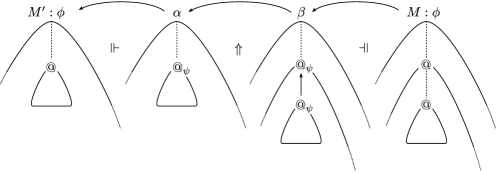
Figure 9: How the compression of terms is able to follow the compression of blueprints.

• If $M$ is of blueprint $\beta$ and $\alpha$ is a vertical compression of $\beta$, the compression of $\beta$ into $\alpha$ can be mimicked by a compression of $M$ into an HRM-term, in the following sense. Assuming $\alpha=\beta[a\leftarrow{\beta}_{|b}]$ (the base case), the term $Q=M[a\leftarrow{M}_{|b}]$ is not in general an HRM-term. However, there exists an HRM-term $M^{\prime}$ with the same domain as $Q$ and of the same type as $M$. Moreover $M^{\prime}$ and $M$ are applications of the same type or abstractions of the same type.

Let us again consider a $\Lambda_{\mbox{\rm\scriptsize NF}}$-inhabitant $M$ and two addresses $a,b$ such that $a<b$, ${M}_{|a}$ and ${M}_{|b}$ are applications of the same type or abstractions of the same type. Suppose:

• there exists a vertical compression $\alpha^{\prime}$ of the blueprint of ${M}_{|b}$ such that the sequence $\Omega(\mbox{\sf Free}({M}_{|a}))$ can be extracted from $\alpha^{\prime}$.

This situation is a generalisation of the last example in the introduction of Section 2 (in which $\alpha^{\prime}$ was equal to the blueprint of ${M}_{|b}$, thereby a trivial compression of this blueprint). The term $M$ is not minimal. Indeed, the key property above implies the existence of a term $N$ of blueprint $\alpha^{\prime}$ whose size is not greater than the size of ${M}_{|b}$, and such that $N,{M}_{|b},{M}_{|a}$ are applications of the same type or abstractions of the same type. By Lemma 2.19, there exists a term $P$ of the same type and with the same domain as $N$ such that $\mbox{\sf Free}(P)=\mbox{\sf Free}({M}_{|a})$. The graft of $P$ at $a$ yields an inhabitant of strictly smaller size.

We will call compact all inhabitants in which the preceding situation does not occur. All inhabitants of minimal size are of course compact. As we shall see in Section 5, we will not need a sharper characterisation of minimal inhabitants. For every formula $\phi$, the set of compact inhabitants of $\phi$ is actually a finite set, and our decision method will consist in the exhaustive computation of their domains.

3.1 Depths of the blueprints of minimal inhabitants

Definition 3.1.

Two terms $M,M^{\prime}\in\Lambda_{\mbox{\rm\scriptsize NF}}$ are of the same kind if and only if they are both variables, or both applications, or both abstractions, and if they are of the same type.

Definition 3.2.

For all formulas $\phi$, we write $\mbox{\sf Sub}(\phi)$ for the set of all subformulas of $\phi$.

Definition 3.3.

Let $M\in\Lambda_{\mbox{\rm\scriptsize NF}}$. Let $a$ be any address in $M$. Let $(a_{1},\dots,a_{m})$ be the strictly increasing sequence of all prefixes of $a$. Let $(\lambda x_{1},\dots,\lambda x_{k})$ be the subsequence of $(M(a_{1}),\dots,M(a_{m}))$ consisting of all labels of the form $\lambda x$. We write $\Lambda(M,a)$ for $(x_{1},\dots,x_{k})$.

Definition 3.4.

Let $M$ be a $\Lambda_{\mbox{\rm\scriptsize NF}}$-inhabitant of $\phi$. We say that $M$ is locally compact if for all addresses $a$ in $M$, the blueprint of ${M}_{|a}$ is of relative depth at most $|\Lambda(M,a)|\times|\mbox{\sf Sub}(\phi)|$.

Lemma 3.5.

Let $M$ be a $\Lambda_{\mbox{\rm\scriptsize NF}}$-inhabitant of $\phi$. If $M$ is not locally compact, then there exist two addresses $b$, $b^{\prime}$ such that $b<b^{\prime}$, ${M}_{|b}$ and ${M}_{|b^{\prime}}$ are of the same kind and $\mbox{\sf Free}({M}_{|b})=\mbox{\sf Free}({M}_{|b^{\prime}})$. Moreover, $M$ is not a $\Lambda_{\mbox{\rm\scriptsize NF}}$-inhabitant of $\phi$ of minimal size.

Proof 3.6.

Figure 10: Proof of Lemma 3.5.

For each address $a$ in ${\mbox{\rm dom}}(M)$, let $\alpha_{a}$ be the blueprint of ${M}_{|a}$ and let $X_{a}=\mbox{\sf Free}({M}_{|a})$. Assume the existence of an $\alpha_{a}$ of relative depth $n>|\Lambda(M,a)|\times|\mbox{\sf Sub}(\phi)|$. There exist $b_{1},\dots,b_{n+1}\in{\mbox{\rm dom}}(\alpha_{a})$ such that $b_{1}<\dots<b_{n}<b_{n+1}$. By Lemma 2.8.(1) we have $X_{a\cdot b_{n}}\subseteq\dots\subseteq X_{a\cdot b_{1}}\subseteq\Lambda(M,a)$. By Lemma 1.5, each $\phi_{a\cdot b_{i}}$ is a subformula of $\phi$. Hence there exist $i,j$ such that $i<j$ and $(X_{a\cdot b_{i}},\phi_{a\cdot b_{i}})=(X_{a\cdot b_{j}},\phi_{a\cdot b_{j}})$, that is, ${M}_{|a\cdot b_{i}}$ and ${M}_{|a\cdot b_{j}}$ are applications of the same type and with the same free variables (Figure 10). Now, let $M^{\prime}=M[a\cdot b_{i}\leftarrow{M}_{|a\cdot b_{j}}]$. The term $M^{\prime}$ is a $\Lambda_{\mbox{\rm\scriptsize NF}}$-inhabitant of $\phi$ of strictly smaller size.

3.2 Vertical compression of a blueprint

Definition 3.7.

We let $\Uparrow$ be the least reflexive and transitive binary relation on blueprints satisfying the following: if $a,b\in{\mbox{\rm dom}}(\beta)$, $a<b$ and $\beta(a)=\beta(b)$, then $\beta[a\leftarrow{\beta}_{|b}]\Uparrow\beta$.

Lemma 3.8.

Suppose $M\in\Lambda_{\mbox{\rm\scriptsize NF}}$, $M:\phi$, $M\Vdash\beta$ and $\alpha\Uparrow\beta$. There exists a term $M^{\prime}\in\Lambda_{\mbox{\rm\scriptsize NF}}$ of the same kind as $M$, of blueprint $\alpha$ and such that $|{\mbox{\rm dom}}(M^{\prime})|\leq|{\mbox{\rm dom}}(M)|$.

Proof 3.9.

It suffices to consider the case of $\alpha=\beta[a\leftarrow{\beta}_{|b}]$ with $a,b\in{\mbox{\rm dom}}(\beta)$, $a<b$ and $\beta(a)=\beta(b)$. We prove the existence of $M^{\prime}$ by induction on the length of $a$. If $a=\varepsilon$ then $M$ is necessarily an application and $\beta(\varepsilon)=\beta(b)=@_{\phi}$, hence ${M}_{|b}$ is an application of type $\phi$, and we can take $M^{\prime}={M}_{|b}$. Assume $a\neq\varepsilon$.

(1) Suppose $M=(M_{1}M_{2})$, $M_{1}\Vdash\beta_{1}$, $M_{2}\Vdash\beta_{2}$, $a=(i)\cdot a_{i}$ and $b=(i)\cdot b_{i}$. By induction hypothesis there exists $M^{\prime}_{i}$ of blueprint $\alpha_{i}=\beta_{i}[a_{i}\leftarrow{\beta_{i}}_{|b_{i}}]=\beta_{i}[a_{i}\leftarrow{\beta}_{|b}]$, of the same kind as $M_{i}$ and such that ${\mbox{\rm dom}}(M^{\prime}_{i})\leq{\mbox{\rm dom}}(M_{i})$. Let $j=1$ if $i=2$, otherwise let $j=2$. Let $(M^{\prime}_{j},\alpha_{j})=(M_{j},\beta_{j})$. Let $X=(x_{1},\dots,x_{n})$ be the strictly increasing sequence of all variables free or bound in $M^{\prime}_{2}$. Let $Y=(y_{1},\dots,y_{n})$ be a strictly increasing sequence of variables such that $\Omega(X)=\Omega(Y)$ and $y_{1}$ is greater that or equal to the greatest variable of $M^{\prime}_{1}$. Let $M^{\prime\prime}_{2}$ be the term obtained by replacing each $x_{i}$ by $y_{i}$ in $M^{\prime}_{2}$. We can take $M^{\prime}=(M^{\prime}_{1}M^{\prime\prime}_{2})$.

(2) Suppose $M=\lambda x.M_{1}$, $M_{1}\Vdash\beta_{1}$, $x:\chi$, $a=(1)\cdot a_{1}$ and $b=(1)\cdot b_{1}$. As $a,b\in{\mbox{\rm dom}}(\beta)$, we have also $a_{1},b_{1}\in{\mbox{\rm dom}}(\beta_{1})$. By induction hypothesis there exists $M^{\prime}_{1}$ of the same kind as $M_{1}$, of blueprint $\alpha_{1}=\beta_{1}[a_{1}\leftarrow{\beta_{1}}_{|b_{1}}]$ and such that ${\mbox{\rm dom}}(M^{\prime}_{1})\leq{\mbox{\rm dom}}(M_{1})$. By Lemma 2.17.(2.a) there exist $\gamma_{1},c_{0},\dots,c_{p}$ such that $\{c_{0},\dots,c_{p}\}=\{c\,|\,{M}_{|c}=x\}$, $\beta_{1}\rhd^{c_{0}}_{\chi}\dots\rhd^{c_{p}}_{\chi}\gamma_{1}$ and $\beta=*(\gamma_{1})$. Since $a,b\in{\mbox{\rm dom}}(\alpha)$, $a_{1}$ and $c_{i}$ are incomparable addresses for all $i$. Hence $\alpha_{1}=\beta_{1}[a_{1}\leftarrow{\beta_{1}}_{|b_{1}}]\rhd^{c_{0}}_{\chi}\dots\rhd^{c_{p}}_{\chi}\gamma_{1}[a_{1}\leftarrow{\beta_{1}}_{|b_{1}}]={\beta[a\leftarrow{\beta}_{|b}]}_{|(1)}={\alpha}_{|1}$. By Lemma 2.19 there exists a term $M^{\prime\prime}_{1}$ of the same type and with the same domain as $M^{\prime}_{1}$ such that the greatest variable $y$ free in $M^{\prime\prime}_{1}$ is of type $\chi$ and $\{c\,|\,{M^{\prime\prime}_{1}}_{|c}=y\}=\{c_{0},\dots,c_{p}\}$. By Lemma 2.17.(2.b) we have $\lambda y.M^{\prime\prime}_{1}\Vdash\alpha$, hence we may take $M^{\prime}=\lambda y.M^{\prime\prime}_{1}$.

Definition 3.10.

A term $M\in\Lambda_{\mbox{\rm\scriptsize NF}}$ is compact when there are no $a,b,\alpha^{\prime}$ such that $a<b$, ${M}_{|a}$ and ${M}_{|b}$ are of the same kind, ${M}_{|b}\Vdash\alpha_{b}$, $\alpha^{\prime}\Uparrow\alpha_{b}$ and $\Omega(\mbox{\sf Free}({M}_{|a}))\in{{\mathbb{F}}\,}(\alpha^{\prime})$.

Lemma 3.11.

Every $\Lambda_{\mbox{\rm\scriptsize NF}}$-inhabitant of minimal size is compact. Every compact $\Lambda_{\mbox{\rm\scriptsize NF}}$-inhabitant of $\phi$ is locally compact.

Proof 3.12.

Let $M$ by an arbitrary $\Lambda_{\mbox{\rm\scriptsize NF}}$-inhabitant of $\phi$.

(1) Assume $M$ is not compact. Let $a,b$ be such that $a<b$, ${M}_{|a}$ and ${M}_{|b}$ are of the same kind, ${M}_{|b}\Vdash\alpha_{b}$, $\alpha^{\prime}\Uparrow\alpha_{b}$, $\mbox{\sf Free}({M}_{|a})=X_{a}$ and $\Omega(X_{a})\in{{\mathbb{F}}\,}(\alpha^{\prime})$ (see Figure 11). By Lemma 3.8 there exists a term $N\in\Lambda_{\mbox{\rm\scriptsize NF}}$ of blueprint $\alpha^{\prime}$, of the same kind as ${M}_{|b}$ and such that $|{\mbox{\rm dom}}(N)|\leq|{\mbox{\rm dom}}({M}_{|b})|$. By Lemma 2.19 there exists $P\in\Lambda_{\mbox{\rm\scriptsize NF}}$ of blueprint $\alpha^{\prime}$, of the same kind as $N$, such that ${\mbox{\rm dom}}(P)={\mbox{\rm dom}}(N)$ and $\mbox{\sf Free}(P)=X_{a}$. The term $M[a\leftarrow P]$ is then a $\Lambda_{\mbox{\rm\scriptsize NF}}$-inhabitant of $\phi$ of smaller size.

(2) Suppose $M$ meets the conditions of Lemma 3.5. Let $\alpha_{b^{\prime}}$ be the blueprint of ${M}_{|b^{\prime}}$. By Lemma 2.17.(3) we have $\Omega(\mbox{\sf Free}({M}_{|b}))=\Omega(\mbox{\sf Free}({M}_{|b^{\prime}})\in{{\mathbb{F}}\,}(\alpha_{b^{\prime}})$. Since the relation $\Uparrow$ is reflexive, $M$ is not compact.

Figure 11: Proof of Lemma 3.11, part (1).

4 Shadows

So far we have isolated two properties shared by all minimal inhabitants (Lemma 3.11). We shall now exploit these properties so as to design a decision method for the inhabitation problem.

In Section 4.1 and 4.2 we show how to associate, with each locally compact inhabitant $M$ of a formula $\phi$, a tree with the same domain as $M$ which we call the shadow of $M$. At each address $a$ this tree is labelled with a triple of the form $(\overline{\chi}_{a},\gamma_{a},\phi_{a})$ where $\phi_{a}$ is the type of ${M}_{|a}$, the sequence $\overline{\chi}_{a}$ is $\Omega(\mbox{\sf Free}({M}_{|a}))$, and $\gamma_{a}$ is a “transversal compression” of the blueprint $\alpha_{a}$ of ${M}_{|a}$ (Definitions 4.1 and 4.2). Recall that $\overline{\chi}_{a}\in{{\mathbb{F}}\,}(\alpha_{a})$ (by Lemma 2.17.(3)). The blueprint $\gamma_{a}$ can be seen as a synthesized version of $\alpha_{a}$ of the same relative depth but of smaller “width”, and such that $\overline{\chi}_{a}\in{{\mathbb{F}}\,}(\gamma_{a})\subseteq{{\mathbb{F}}\,}(\alpha_{a})$.

Each tree prefix of the shadow of $M$ belongs to a finite set effectively computable from $\phi$ and the domain of this prefix. In particular, one can compute all possible values for its labels, regardless of the full knowledge of $M$ – or even without the knowledge of the existence of $M$. The key property satisfied by this shadow at every address $a$ is:

• for each $\gamma^{\prime}\Uparrow\gamma_{a}$, there exists $\alpha^{\prime}\Uparrow\alpha_{a}$ such that ${{\mathbb{F}}\,}(\gamma^{\prime})\subseteq{{\mathbb{F}}\,}(\alpha^{\prime})$.

This property is sufficient to detect the non-compactness of $M$ for a pair of addresses $(a,b)$ only from the knowledge of $\overline{\chi}_{a},\phi_{a},\gamma_{b},\phi_{b}$ and the arity of the nodes at $a$ and $b$. Indeed, suppose $a<b$, $\phi_{a}=\phi_{b}$ and the nodes at $a$, $b$ are of the same arity (1, or 2). Now, assume:

• there exists $\gamma^{\prime}\Uparrow\gamma_{b}$ such that $\overline{\chi}_{a}\in{{\mathbb{F}}\,}(\gamma^{\prime})$.

Then ${M}_{|a}$ and ${M}_{|b}$ are of the same kind and there exists $\alpha^{\prime}\Uparrow\alpha_{b}$ such that $\overline{\chi}_{a}=\Omega(\mbox{\sf Free}({M}_{|a}))\in{{\mathbb{F}}\,}(\gamma^{\prime})\subseteq{{\mathbb{F}}\,}(\alpha^{\prime})$, therefore $M$ is not compact.

In Section 4.2, what we call a shadow is merely a tree $a\mapsto(\overline{\chi}_{a},\gamma_{a},\phi_{a})$ of a certain shape, no matter if this tree is the shadow of a term or not. This shadow is compact if there is no pair ($a,b$) as above. Of course, the shadow of a compact term is always compact in this sense.

In Section 5 we will prove that for every formula $\phi$, the set of shadows of compact inhabitants of $\phi$ is a finite set effectively computable from $\phi$ (hence the same property holds for the set of compact inhabitants of $\phi$), and we will deduce from this key property the decidability of type inhabitation for HRM-terms.

4.1 Blueprint equivalence and transversal compression

Definition 4.1.

We let $\equiv$ be the least binary relation on blueprints such that:

1. $\emptyset_{\,{\mathbb{B}}\,}\equiv\emptyset_{\,{\mathbb{B}}\,}$,

2. $\phi\equiv\phi$,

3. if $\alpha_{1}\equiv\beta_{1}$, $\alpha_{2}\equiv\beta_{2}$, then $@_{\phi}(\alpha_{1},\alpha_{1})\equiv@_{\phi}(\beta_{1},\beta_{2})$,

4. if $|\overline{a}|=|\overline{b}|=n$ and $\alpha_{i}\equiv\beta_{i}$ for each $i\in[1,\dots,n]$, then $*_{\overline{a}}(\alpha_{1},\dots,\alpha_{n})\equiv*_{\overline{b}}(\beta_{1},\dots,\beta_{n})$.

In (3), we assume $\alpha_{1},\alpha_{2},\beta_{1},\beta_{2}$ non-empty. In (4), we assume that the elements of each sequence $\overline{a}$, $\overline{b}$ are pairwise incomparable addresses. As to avoid circularity we assume also $a\neq\varepsilon$ or $b\neq\varepsilon$, and $\alpha_{i},\beta_{i}\neq\emptyset_{\,{\mathbb{B}}\,}$ for at least one $i$.

To some extent this equivalence allows us to consider blueprints regardless of the exact values of addresses. For instance $*_{\overline{a}}(\alpha_{1},\dots,\alpha_{n})\equiv*(\alpha_{1},\dots,\alpha_{n})\equiv*(\alpha_{n},\dots,\alpha_{1})$, also $*(*(\alpha,\beta),\gamma)\equiv*(\alpha,\beta,\gamma)\equiv*(\alpha,*(\beta,\gamma))$, etc. It is easy to check that $\alpha\equiv\beta$ implies ${{\mathbb{F}}\,}(\alpha)={{\mathbb{F}}\,}(\beta)$ – this property will be used without reference.

Definition 4.2.

For each $m\in{\rm Nature}$, we let $\curvearrowleft_{m}$ be the least binary relation such that:

1. if $\gamma_{1}\equiv\dots\equiv\gamma_{m}\equiv\gamma_{m+1}\not\equiv\emptyset_{\,{\mathbb{B}}\,}$, then $\ast_{\overline{a}}(\gamma_{1},\dots,\gamma_{m})\curvearrowleft_{m}\ast_{\overline{a}\cdot(b)}(\gamma_{1},\dots,\gamma_{m},\gamma_{m+1})$,

2. if $\alpha=*_{\overline{a}}(\alpha_{1},\dots,\alpha_{n})$, $\beta=*_{\overline{b}}(\beta_{1},\dots,\beta_{p})$ and $\alpha\curvearrowleft_{m}\beta$, then:

   1. $@_{\phi}(\alpha,\gamma)\curvearrowleft_{m}@_{\phi}(\beta,\gamma)$,

   2. $@_{\phi}(\gamma,\alpha)\curvearrowleft_{m}@_{\phi}(\gamma,\beta)$,

   3. $\ast_{\overline{a}\cdot(c)}(\alpha_{1},\dots,\alpha_{n},\gamma)\curvearrowleft_{m}\ast_{\overline{b}\cdot(c)}(\beta_{1},\dots,\beta_{p},\gamma)$.

We call $m$-compression of $\beta$ every $\alpha$ such that $\alpha\curvearrowleft_{m}\beta$. The width of $\beta$ is defined as the least $m\in{\rm Nature}$ for which there is no $\alpha$ such that $\alpha\curvearrowleft_{m}\beta$.

Again the elements of $\overline{a}\cdot(b)$, $\overline{a}\cdot(c)$ and $\overline{b}\cdot(c)$ must be pairwise incomparable addresses, and $\alpha,\beta,\gamma$ must be non-empty. Note that for all non-empty $\beta$, we have $\emptyset_{\,{\mathbb{B}}\,}\curvearrowleft_{0}\beta$, hence the empty blueprint is the only blueprint of null width. If $\beta$ is of width $m>0$, then for all addresses $a$, for ${\beta}_{|a}=\ast_{\overline{a}}(\gamma_{1},\dots,\gamma_{k})$ and for each $\gamma_{i}\neq\emptyset_{\,{\mathbb{B}}\,}$, the sequence $(\gamma_{1},\dots,\gamma_{k})$ contains no more than $m$ blueprints $\equiv$-equivalent to $\gamma_{i}$. For instance, if $\phi,\psi,\chi$ are distinct formulas, $\ast(\phi,\phi,\phi,\psi,\psi,\chi)$ is of width 3, $\ast(\omega,@_{\omega}(*(\phi,\psi),\phi),@_{\omega}(*(\psi,\phi),\phi))$ is of width 2, etc.

Definition 4.3.

For each $m\in{\rm Nature}$, we write $\sqsubseteq_{m}$ for the reflexive and transitive closure of the union of $\equiv$ and $\curvearrowleft_{m}$. We let $\sqsubseteq^{\max}_{m}$ denote the subset of the relation $\sqsubseteq_{m}$ of all pairs with a left-hand-side of width at most $m$.

For instance, if $\phi,\psi,\chi$ are distinct formulas:

$$\emptyset_{\,{\mathbb{B}}\,}\sqsubseteq^{\max}_{0}\ast(\psi,\chi,\phi)\sqsubseteq^{\max}_{1}\ast(\chi,\phi,\phi,\psi,\psi)\sqsubseteq^{\max}_{2}\ast(\phi,\phi,\phi,\psi,\psi,\chi)$$

Of course $\alpha\sqsubseteq_{m}\beta$ implies $\alpha\sqsubseteq_{j}\beta$ for all $j\in[1,\dots,m]$ and clearly, $\alpha\curvearrowleft_{m}\beta$ implies $|{\mbox{\rm dom}}(\alpha)|<|{\mbox{\rm dom}}(\beta)|$, therefore $\curvearrowleft_{m}$ is well-founded.

Definition 4.4.

For all ${\cal S}\subseteq{\mathfrak{S}}$, for all $d\in{\rm Nature}$ and for all $m\in{\rm Nature}$:

• we let ${{\mathbb{B}}\hskip 0.86108pt}({\cal S},d,\infty)$ be the set of ${\cal S}$-blueprints of relative depth at most $d$,

• we let ${{\mathbb{B}}\hskip 0.86108pt}({\cal S},d,m)$ be the set of all blueprints in ${{\mathbb{B}}\hskip 0.86108pt}({\cal S},d,\infty)$ of width at most $m$.

Lemma 4.5.

For all finite ${\cal S}\subseteq{\mathfrak{S}}$, for all $d\in{\rm Nature}$ and for all $m\in{\rm Nature}$:

1. The set ${{\mathbb{B}}\hskip 0.86108pt}({\cal S},d,m)/_{\equiv}$ is a finite set.

2. A selector ${{\mathbb{R}}\,}({\cal S},d,m)$ for ${{\mathbb{B}}\hskip 0.86108pt}({\cal S},d,m)/_{\equiv}$ is effectively computable from $({\cal S},d,m)$.

Proof 4.6.

(1) Let ${{\mathbb{B}}\hskip 0.86108pt}_{\varepsilon}({\cal S},d,m)$ be the set of all rooted blueprints in ${{\mathbb{B}}\hskip 0.86108pt}({\cal S},d,m)$. Assuming ${{\mathbb{B}}\hskip 0.86108pt}_{\varepsilon}({\cal S},d,m)/_{\equiv}$ is a finite set and a selector ${{\mathbb{R}}\,}_{\varepsilon}({\cal S},d,m)$ for ${{\mathbb{B}}\hskip 0.86108pt}_{\varepsilon}({\cal S},d,m)/_{\equiv}$ is effectively computable from $({\cal S},d,m)$, we prove that ${{\mathbb{B}}\hskip 0.86108pt}({\cal S},d,m)/_{\equiv}$ and ${{\mathbb{B}}\hskip 0.86108pt}_{\varepsilon}({\cal S},d+1,m)/_{\equiv}$ are finite sets and show how to compute a selector for each set.

Let $(\alpha_{1},\dots,\alpha_{k})$ be an enumeration of ${{\mathbb{R}}\,}_{\varepsilon}({\cal S},d,m)$. Let $\Sigma_{d}$ be the set of all functions from $\{1,\dots,k\}$ to $\{0,\dots,m\}$. For each $\beta\in{{\mathbb{B}}\hskip 0.86108pt}({\cal S},d,m)$ there exist $\beta_{1},\dots,\beta_{n}\in{{\mathbb{B}}\hskip 0.86108pt}_{\varepsilon}({\cal S},d,m)$ and $\overline{b}$ such that $\beta=*_{\overline{b}}(\beta_{1},\dots,\beta_{n})$. We let $\sigma_{\beta}$ be the function mapping each $i\in\{1,\dots,k\}$ to the number of occurrences of an element $\equiv$-equivalent to $\alpha_{i}$ in the sequence $(\beta_{1},\dots,\beta_{n})$. Clearly $\sigma_{\beta}\in\Sigma_{d}$ and furthermore for all $\beta^{\prime}\in{{\mathbb{B}}\hskip 0.86108pt}({\cal S},d,m)$ we have $\beta\equiv\beta^{\prime}$ if and only if $\sigma_{\beta}=\sigma_{\beta^{\prime}}$, hence ${{\mathbb{B}}\hskip 0.86108pt}({\cal S},d,m)$ is a finite set.

For each $\tau\in\Sigma_{d}$, let $\rho_{\tau}=*(\alpha^{1}_{1},\dots,\alpha^{\tau(1)}_{1},\dots,\alpha^{1}_{k},\dots,\alpha^{\tau(k)}_{k})$ where each $\alpha^{j}_{i}$ is equal to $\alpha_{i}$. We have $\rho_{\tau}\in{{\mathbb{B}}\hskip 0.86108pt}({\cal S},d,m)$ and $\sigma(\rho_{\tau})=\tau$, that is, if $\tau,\tau^{\prime}\in\Sigma_{d}$ and $\tau\neq\tau^{\prime}$, then $\rho_{\tau}\not\equiv\rho_{\tau^{\prime}}$. Hence we may define ${{\mathbb{R}}\,}({\cal S},d,m)$ as $\{\rho_{\tau}\,|\,\tau\in\Sigma_{d}\}$.

The finiteness of ${{\mathbb{B}}\hskip 0.86108pt}_{\varepsilon}({\cal S},d+1,m)/_{\equiv}$ follows immediately from the finiteness of ${{\mathbb{B}}\hskip 0.86108pt}({\cal S},d,m)$ and the fact that if $\beta=@_{\phi}(\beta_{1},\beta_{2})$ and $\beta^{\prime}=@_{\psi}(\beta^{\prime}_{1},\beta^{\prime}_{2})$ are elements of ${{\mathbb{B}}\hskip 0.86108pt}_{\varepsilon}({\cal S},d+1,m)$, then $\beta_{1},\beta_{2},\beta^{\prime}_{1},\beta^{\prime}_{2}$ are non-empty elements of ${{\mathbb{B}}\hskip 0.86108pt}({\cal S},d,m)$ and furthermore $\beta\equiv\beta^{\prime}$ if and only if $\beta_{1}\equiv\beta^{\prime}_{1}$ and $\beta_{2}\equiv\beta^{\prime}_{2}$. The same property allows us to define ${{\mathbb{R}}\,}_{\varepsilon}({\cal S},d+1,m)$ as the set of all blueprints of the form $@_{\phi}(\gamma_{1},\gamma_{2})$ where $@_{\phi}\in S$ and each $\gamma_{i}$ is a non-empty element of ${{\mathbb{R}}\,}({\cal S},d,m)$.

(2) The lemma follows by induction on $d$, using (1) and the facts that: ${{\mathbb{B}}\hskip 0.86108pt}_{\varepsilon}({\cal S},0,0)$ is empty (hence ${{\mathbb{B}}\hskip 0.86108pt}({\cal S},d,0)=\{\emptyset_{\,{\mathbb{B}}\,}\}$ for all $d$); if $m\in{\rm Nature}_{+}$, then ${{\mathbb{B}}\hskip 0.86108pt}_{\varepsilon}({\cal S},0,m)$ is the finite set of all formulas of ${\cal S}$.

4.2 Shadow of a term

Definition 4.7.

Let $\phi$ be a formula. Let ${\cal S}_{\phi}$ be the union of $\mbox{\sf Sub}(\phi)$ (Definition 3.2) and the set of all $@_{\psi}$ such that $\psi\in\mbox{\sf Sub}(\phi)$. For each integer $k$, for each formula $\phi$, we let ${\mathfrak{R}}(\phi,k)={{\mathbb{R}}\,}({\cal S}_{\phi},k\times|\mbox{\sf Sub}(\phi)|,k)$, where ${{\mathbb{R}}\,}$ is the function introduced in Lemma 4.5.(2).

Definition 4.8.

A shadow is a finite tree in which each node is of arity at most 2 and is labelled with a triple of the form $(\overline{\chi},\gamma,\psi)$, where $\overline{\chi}$ is a sequence of formulas, $\gamma$ is a blueprint and $\psi$ is a formula.

We call $\phi$-shadow every shadow $\Xi$ satisfying the following conditions. We have $\Xi(\varepsilon)=(\varepsilon,\emptyset_{\,{\mathbb{B}}\,},\phi)$. For each $a\in{\mbox{\rm dom}}(\Xi)$, let $k_{a}$ be the number of $b<a$ such that the node of $\Xi$ at $b$ is unary, and let $(\overline{\chi}_{a},\gamma_{a},\psi_{a})=\Xi(a)$. Then:

• $\overline{\chi}_{a}$ is a sequence of subformulas of $\phi$ of length at most $k_{a}$,

• $\gamma_{a}\in{\mathfrak{R}}(\phi,k_{a})$,

• $\overline{\chi}_{a}\in{{\mathbb{F}}\,}(\gamma_{a})$

• $\psi_{a}$ is a subformula of $\phi$.

Definition 4.9.

Let $M$ be a locally compact $\Lambda_{\mbox{\rm\scriptsize NF}}$-inhabitant of $\phi$. For each $a\in{\mbox{\rm dom}}(M)$:

• let $\overline{\chi}_{a}=\Omega(\mbox{\sf Free}({M}_{|a}))$,

• let $\alpha_{a}$ be the blueprint of ${M}_{|a}$,

• let $\gamma_{a}\in{\mathfrak{R}}(\phi,|\Lambda(M,a)|)$ be such that $\gamma_{a}\sqsubseteq^{\max}_{|\Lambda(M,a)|}\alpha_{a}$,

• let $\phi_{a}$ be the type of ${M}_{|a}$.

The tree $\Xi$ mapping each $a\in{\mbox{\rm dom}}(M)$ to $(\overline{\chi}_{a}.\gamma_{a},\phi_{a})$ will be called the shadow of $M$.

Recall that if $M$ is a locally compact $\Lambda_{\mbox{\rm\scriptsize NF}}$-inhabitant of $\phi$, then for each address $a$ in $M$, the blueprint $\alpha_{a}$ of ${M}_{|a}$ is of relative depth at most $|\Lambda(M,a)|\times|\mbox{\sf Sub}(\phi)|$. Every maximal $|\Lambda(M,a)|$-compression of $\alpha_{a}$ produces a shadow $\alpha^{\prime}_{a}$ with the same relative depth and of width at most $|\Lambda(M,a)|$, to which some element of ${\mathfrak{R}}(\phi,|\Lambda(M,a)|)$ is equivalent, thus the shadow of $M$ is well-defined. Note that the choice of $\gamma_{a}$ is possibly not unique (although it is, since ${\mathbb{R}}$ is a selector and one can actually prove that $\gamma\sqsubseteq^{\max}_{m}\alpha$ and $\gamma^{\prime}\sqsubseteq^{\max}_{m}\alpha$ implies $\gamma\equiv\gamma^{\prime}$, but this property is irrelevant to our discussion). We assume that some $\gamma_{a}$ is chosen for each address $a$ in $M$.

Obviously the shadow of $M$ satisfies the first, second and fourth conditions in the definition of $\phi$-shadows given above – in the next section, we prove that it satisfies also the third.

Figure 12: A compact inhabitant and its shadow.

4.3 Compact shadows and compact inhabitants

Definition 4.10.

A shadow $\Xi$ is compact if and only if there are no $a,b$ such that: $a<b$, the nodes of $\Xi$ at $a$, $b$ are of the same arity, $\Xi(a)=(\overline{\chi}_{a},\gamma_{a},\psi)$, $\Xi(b)=(\overline{\chi}_{b},\gamma_{b},\psi)$ and there exists $\gamma^{\prime}\Uparrow\gamma_{b}$ such that $\overline{\chi}_{a}\in{{\mathbb{F}}\,}(\gamma^{\prime})$.

Compare this definition with the definition of compactness for term (Definition 3.10). With the help of three auxiliary lemmas, we now prove the key lemma of Section 4: if $M$ is a compact inhabitant – a fortiori locally compact by Lemma 3.11 – then the shadow of $M$ is a compact $\phi$-shadow.

Lemma 4.11.

If $\alpha\Uparrow\beta\sqsubseteq_{1}\beta^{\prime}$, then there exists $\alpha^{\prime}$ such that $\alpha\sqsubseteq_{1}\alpha^{\prime}\Uparrow\beta^{\prime}$.

Proof 4.12.

(1) An immediate induction on $|{\mbox{\rm dom}}(\beta^{\prime})|$ shows that if $\alpha=\beta[a\leftarrow{\beta}_{|b}]$ and $\beta\equiv\beta^{\prime}$, then there exist $a^{\prime},b^{\prime}$ such that $a^{\prime}<b^{\prime}$ and $\alpha\equiv\alpha^{\prime}=\beta^{\prime}[a^{\prime}\leftarrow{\beta^{\prime}}_{|b^{\prime}}]$. As a consequence, an immediate induction on the length of the derivation of $\alpha\Uparrow\beta$ shows that the lemma holds if $\beta\equiv\beta^{\prime}$.

(2) Another induction on $|{\mbox{\rm dom}}(\beta^{\prime})|$ shows that if $\alpha\Uparrow\beta\curvearrowleft_{1}\beta^{\prime}$, then there exists $\alpha^{\prime}$ such that $\alpha\curvearrowleft_{1}\alpha^{\prime}\Uparrow\beta^{\prime}$. The only non trivial case is $\alpha=\ast_{(a_{1})}(\alpha_{1})$, $\beta=*_{(a_{1})}(\beta_{1})$ with $\alpha_{1}\Uparrow\beta_{1}$ and $\beta^{\prime}=*_{(a_{1},a_{2})}(\beta_{1},\beta_{2})$ with $\beta_{1}\equiv\beta_{2}$. Since $\alpha_{1}\Uparrow\beta_{1}\equiv\beta_{2}$, by (1) there exists $\alpha_{2}$ such that $\alpha_{1}\equiv\alpha_{2}\Uparrow\beta_{2}$. Hence $\alpha=\ast_{(a_{1})}(\alpha_{1})\curvearrowleft_{1}\ast_{(a_{1},a_{2})}(\alpha_{1},\alpha_{2})\Uparrow\ast_{(a_{1},a_{2})}(\beta_{1},\beta_{2})=\beta^{\prime}$.

(3) Using (1) and (2), the lemma follows by induction on the length of an arbitrary sequence $(\beta_{0},\dots,\beta_{n})$ such that $\beta_{0}=\beta$, $\beta_{n}=\beta^{\prime}$ and $\beta_{i-1}\equiv\beta_{i}$ or $\beta_{i-1}\curvearrowleft_{1}\beta_{i}$ for each $i\in[1,\dots,n]$.

Lemma 4.13.

If $\alpha\sqsubseteq_{1}\beta$, then ${{\mathbb{F}}\,}(\alpha)\subseteq{{\mathbb{F}}\,}(\beta)$.

Proof 4.14.

By induction on $|{\mbox{\rm dom}}(\beta)|$. Since $\gamma\equiv\gamma^{\prime}$ implies ${{\mathbb{F}}\,}(\gamma)={{\mathbb{F}}\,}(\gamma^{\prime})$ and $|{\mbox{\rm dom}}(\gamma)|=|{\mbox{\rm dom}}(\gamma^{\prime})|$, it suffices to consider the case where $\alpha$ is a $1$-compression of $\beta$. The case $\alpha=*_{(a_{1})}(\alpha_{1})$ and $\beta=*_{(a_{1},a_{2})}(\alpha_{1},\alpha_{2})$ is clear. The remaining cases follow easily from the induction hypothesis.

Lemma 4.15.

If $\alpha\sqsubseteq_{m}\beta$, then the set of all elements of ${{\mathbb{F}}\,}(\beta)$ of length at most $m$ is a subset of ${{\mathbb{F}}\,}(\alpha)$.

Proof 4.16.

By induction on $|{\mbox{\rm dom}}(\beta)|$. Again, we examine only the case $\alpha\curvearrowleft_{m}\beta$. The proposition is trivially true if $m=0$. Suppose $m>0$. The only non-trivial case is $\alpha\equiv*_{\overline{a}}(\gamma_{1},\dots,\gamma_{m})$ and $\beta\equiv*_{\overline{a}}(\gamma_{1},\dots,\gamma_{m},\gamma_{m+1})$ with $\gamma_{i}\equiv\gamma$ for all $i$. Let $\Phi={{\mathbb{F}}\,}(\gamma)$. For each integer $k$, let $\Phi^{(k)}=\circledast(\Phi_{1},\dots,\Phi_{k})$ where $\Phi_{i}={{\mathbb{F}}\,}(\gamma)$ for each $i$. Let $\overline{\phi}=(\phi_{1},\dots,\phi_{p})\in{{\mathbb{F}}\,}(\beta)$ be such that $p\leq m$. We have to prove that $\overline{\phi}\in{{\mathbb{F}}\,}(\alpha)$. For each $J\subseteq\{1,\dots,p\}$, let $(j_{1},\dots,j_{q})$ be the strictly increasing enumeration of all elements of $J$ and let $f(J)=(\phi_{j_{1}},\dots,\phi_{j_{q}})$. We have $\overline{\phi}\in{{\mathbb{F}}\,}(\beta)=\Phi^{(m+1)}$, hence there exist $J_{1},\dots,J_{m+1}$ such that $J_{1}\cup\dots\cup J_{m+1}=\{1,\dots,p\}$, and $f(J_{i})\in{{\mathbb{F}}\,}(\gamma)$ for each $i\in\{1,\dots,m+1\}$. For each $j\in\{1,\dots,p\}$, let $k_{j}$ be any element of $\{1,\dots,m+1\}$ such that $j\in J_{k_{j}}$. Then $J_{k_{1}}\cup\dots\cup J_{k_{p}}=\{1,\dots,p\}$, so $\overline{\phi}\in\circledast(\{f(J_{k_{1}})\},\dots,\{f(J_{k_{p}})\})\subseteq\Phi^{(p)}\subseteq\Phi^{(m)}={{\mathbb{F}}\,}(\alpha)$.

Lemma 4.17.

Let $M$ be a locally compact $\Lambda_{\mbox{\rm\scriptsize NF}}$-inhabitant of $\phi$. The shadow of $M$ is a $\phi$-shadow. If $M$ is compact, then this shadow is also compact.

Proof 4.18.

For each address $a$ in $M$, the sequence $\overline{\chi}_{a}=\Omega(\mbox{\sf Free}({M}_{|a}))$ is a subsequence of $\Omega(\Lambda(M,a))$, hence the first proposition follows from the definition of the shadow of $M$, Lemma 1.5, Lemma 2.17.(3) and Lemma 4.15. Let $\Xi$ be shadow of $M$. Assume $\Xi$ is not compact. There exist $a,b\in{\mbox{\rm dom}}(\Xi)={\mbox{\rm dom}}(M)$ such that $\Xi(a)=(\overline{\chi}_{a},\gamma_{a},\psi)$, $\Xi(b)=(\overline{\chi}_{b},\gamma_{b},\psi)$, the nodes at $a$,$b$ in $\Xi$ are of the same arity, and there exists $\gamma^{\prime}\Uparrow\gamma_{b}$ such that $\overline{\chi}_{a}\in{{\mathbb{F}}\,}(\gamma^{\prime})$. We have ${M}_{|a}$, ${M}_{|b}$ of the same kind. Let $\alpha_{a},\alpha_{b}$ be the blueprints of ${M}_{|a}$, ${M}_{|b}$. Since $\gamma_{b}\sqsubseteq_{|\Lambda(M,a\cdot b)|}^{\max}\alpha_{b}$, we have $\gamma^{\prime}\Uparrow\gamma_{b}\sqsubseteq_{1}\alpha_{b}$. By Lemma 4.11 there exists $\alpha^{\prime}$ such that $\gamma^{\prime}\sqsubseteq_{1}\alpha^{\prime}\Uparrow\alpha_{b}$. By Lemma 4.13, we have $\overline{\chi}_{a}\in{{\mathbb{F}}\,}(\gamma^{\prime})\subseteq{{\mathbb{F}}\,}(\alpha^{\prime})$, hence $M$ is not compact.

5 Finiteness of the set of compact $\phi$-shadows

Our last aim will be to prove that for each formula $\phi$, the set of all compact $\phi$-shadows is a finite set effectively computable from $\phi$.

In definition 5.1, we introduce a last binary relation $\Subset$ on blueprints. The key lemma of this section (Lemma 5.21) shows that whenever ${\cal S}\subset{\mathfrak{S}}$ is a finite set (in particular when ${\cal S}$ is the set of all subformulas of $\phi$ and all $@$’s tagged with a subformula of $\phi$), the relation $\Subset$ is an almost full relation [Bezem, Klop and de Vrijer 2003] on the set of all ${\cal S}$-blueprints: for every infinite sequence $\gamma_{1},\gamma_{2},\dots$ over ${{\mathbb{B}}\hskip 0.86108pt}({\cal S})$, there exists $i,j$ such that $i<j$ and $\gamma_{i}\Subset\gamma_{j}$. This result will be proven with the help of Melliès’ Axiomatic Kruskal Theorem [Melliès 1998]. The finiteness of the set of compact $\phi$-shadows follows from this key lemma with the help of König’s Lemma (Lemma 5.23). The ability to compute these shadows follows directly from their definition.

By Lemma 4.17, a consequence of this result is also the finiteness for each $\phi$ of the set of all compact $\Lambda_{\mbox{\rm\scriptsize NF}}$-inhabitants of $\phi$, although our decision method is based on the computation of shadows of compact terms rather than a direct computation of those terms. It is worth mentioning that the proof of Theorem 5.19 is non-constructive and that it gives no information about the complexity of our proof-search method – this question might be itself another open problem.

5.1 Almost full relations and Higman Theorem

Definition 5.1.

We let $\Subset$ be the relation on blueprints defined by $\alpha\Subset\beta$ if and only if for all $\overline{\chi}\in{{\mathbb{F}}\,}(\alpha)$, there exists $\gamma\Uparrow\beta$ such that $\overline{\chi}\in{{\mathbb{F}}\,}(\gamma)$.

Definition 5.2.

Let $\cal U$ be an arbitrary set. An almost full relation (AFR) on ${\cal U}$ is a binary relation $\ll$ such that for every infinite sequence $(u_{i})_{i\in{\rm Nature}}$ over ${\cal U}$, there exist $i,j$ such that $i<j$ and $u_{i}\ll u_{j}$.

The main aim of Section 5 will be to prove the last key lemma from which we will easily infer the decidability of $\Lambda_{\mbox{\rm\scriptsize NF}}$-inhabitation: for each finite ${\cal S}\subseteq{\mathfrak{S}}$, the relation $\Subset$ is an AFR on ${{\mathbb{B}}\hskip 0.86108pt}({\cal S})$.

Proposition 5.3.

1. If $\ll$ and $\ll^{\prime}$ are AFRs on ${\cal U}$, then $\ll\cap\ll^{\prime}$ is an AFR on ${\cal U}$.

2. Suppose $\ll_{\cal U}$ is an AFR on ${\cal U}$ and $\ll_{\cal V}$ is an AFR on ${\cal V}$. Let $\ll_{{\cal U}\times{\cal V}}$ be the relation defined by $(U,V)\ll_{{\cal U}\times{\cal V}}(U^{\prime},V^{\prime})$ if and only if $U\ll_{\cal U}U^{\prime}$ and $V\ll_{\cal V}V^{\prime}$. Then $\ll_{{\cal U}\times{\cal V}}$ is an AFR on ${\cal U}\times{\cal V}$.

Proof 5.4.

See [Melliès 1998]. Both results appear in the proof of Theorem 1, Step 4 (p.523) as a corollary of Lemma 4 (p.520)

Definition 5.5.

Let ${\cal U}$ be a set, let $\ll$ be a binary relation. We let ${\mathbb{S}}({\cal U})$ denote the set of all finite sequences over ${\cal U}$. The relation $\ll_{\mathbb{S}}$ induced by $\ll$ on ${\mathbb{S}}({\cal U})$ is defined by $(U_{1},\dots,U_{n})\ll_{\mathbb{S}}(V_{1},\dots,V_{m})$ if and only if there exists a strictly monotone function $\eta:\{1,\dots,n\}\to\{1,\dots,m\}$ such that $U_{i}\ll\,V_{\eta(i)}$ for each $i\in\{1,\dots,n\}$.

Theorem 5.6.

(Higman) If $\ll$ is an AFR on ${\cal U}$, then ${\ll}_{\mathbb{S}}$ is an AFR on ${\mathbb{S}}({\cal U})$.

Proof 5.7.

See [Higman 1952, Kruskal 1972, Melliès 1998].

5.2 From rooted to unrooted blueprints

Melliès’ Axiomatic Kruskal Theorem allows one to conclude that a relation is an AFR (a “well binary relation” in [Melliès 1998]) as long as it satisfies a set of five properties or “axioms” (six in the original version of the theorem – see the remarks of Melliès at the end of its proof explaining why five axioms suffice). The details of those axioms will be given in Section 5.3.

Four of those five axioms are relatively easy to check. The remaining axiom is more problematical. This rather technical section is entirely devoted to the proof of Lemma 5.16, which will ensure that this last axiom is satisfied. We want to prove the following proposition:

Let ${\cal S}$ be a finite subset of ${\mathfrak{S}}$. Let ${\cal B}_{\varepsilon}$ be a subset of ${{\mathbb{B}}\hskip 0.86108pt}_{\varepsilon}({\cal S})$.

Let ${\cal B}=\{*_{\overline{a}}(\beta_{1},\dots,\beta_{n})|\,\forall i\in[1,\dots,n],\beta_{i}\in{\cal B}_{\varepsilon}\}$.

If $\Subset$ is an AFR on ${\cal B}_{\varepsilon}$, then $\Subset$ is an AFR on ${\cal B}$.

Recall that ${{\mathbb{B}}\hskip 0.86108pt}_{\varepsilon}({\cal S})$ stands for the set of all rooted ${\cal S}$-blueprints. We want to be able to extend the property that $\Subset$ is an AFR on a given set of rooted blueprints to the set all blueprints that have those rooted blueprints at their minimal addresses.

Higman Theorem suffices to show that $\Subset_{\mathbb{S}}$ (Definition 5.5) is an AFR on the set of finite sequences over ${\cal B}_{\varepsilon}$. However, if one considers an infinite sequence $(\beta_{i})_{i\in{\rm Nature}}$ over ${\cal B}$ and transforms each $\beta_{i}=*_{\overline{a}_{i}}(\beta^{i}_{1},\dots,\beta^{i}_{n_{i}})$ where $\beta^{i}_{1},\dots,\beta^{i}_{n_{i}}\in{\cal B}_{\varepsilon}$ into $\sigma(\beta_{i})=(\beta^{i}_{1},\dots,\beta^{i}_{n_{i}})$, the theorem will only provide two integers $i,j$ and strictly monotone function $\eta$ such that $i<j$ and $\beta^{i}_{k}\Subset\beta^{j}_{\eta(k)}$ for each $k\in\{1,\dots,n_{i}\}$. This is sufficient to ensure that $\beta_{i}=*_{\overline{a}_{i}}(\beta^{i}_{1},\dots,\beta^{i}_{n_{i}})\Subset\ast_{\overline{b}}(\beta^{j}_{\eta(1)},\dots,\beta^{j}_{\eta(n_{i})})$, but not in general $\beta_{i}\Subset\beta_{j}$.

To bypass this difficulty we show how for each blueprint $\beta\in{{\mathbb{B}}\hskip 0.86108pt}({\cal S})$, one can extract from the set of all vertical compressions of $\beta$ a complete set of “followers” of $\beta$ of minimal size (Lemma 5.9). This set $\{\alpha_{1},\dots,\alpha_{p}\}$ has the property that for each $\overline{\phi}\in{{\mathbb{F}}\,}(\beta)$, there exists at least one $\alpha_{i}$ such that ${{\mathbb{F}}\,}(\alpha_{i})$ contains a subsequence of $\overline{\phi}$ – but not necessarily $\overline{\phi}$ itself. The relative depth of each $\alpha_{i}$ does not depend on the relative depth on $\beta$, but only on ${\cal S}$: it is at most $\Sigma_{i=1}^{1+|{\cal S}_{@}|}\,i$, where ${\cal S}_{@}$ is the set of all binary symbols in ${\cal S}$. The lemma in proven in four steps.

First, observe that the set of all $\alpha\Uparrow\beta$ of relative depth at most $\Sigma_{i=1}^{1+|{\cal S}_{@}|}\,i$ is a complete set of followers. If we consider the set of all $\gamma$ such that $\gamma\sqsubseteq^{\max}_{1}\alpha$ for at least one such $\alpha$, we obtain a (possibly infinite) set closed under $\equiv$ and finite up to $\equiv$. We call it the set of ${\cal S}$-residuals of $\beta$.

Second, we prove that the set of ${\cal S}$-residuals of $\beta$ is a complete set of followers of $\beta$ in the same sense, that is, for each $\overline{\phi}\in{{\mathbb{F}}\,}(\beta)$ there exists an ${\cal S}$-residual $\gamma$ of $\beta$ such that ${{\mathbb{F}}\,}(\gamma)$ contains a subsequence of $\overline{\phi}$ (Lemma 5.12).

Third, we prove that if $\beta=*_{\overline{a}}(\beta_{1},\dots,\beta_{n})$, $\beta^{\prime}=*_{\overline{b}}(\beta^{\prime}_{1},\dots,\beta^{\prime}_{n},\beta^{\prime}_{n+1},\dots,\beta^{\prime}_{n+k})$ are such that $\beta_{i}\Subset\beta^{\prime}_{i}$ for each $i\in[1,\dots,n]$, and if furthermore $\beta,\beta^{\prime}$ have the same set of ${\cal S}$-residuals, then $\beta\Subset\beta^{\prime}$ (Lemma 5.14).

The last step is the proof of the lemma itself. The set of ${\cal S}$-residuals is finite up to $\equiv$ (Lemma 4.5), so there are only a finite number of possible values for the set of residuals of each ${\cal S}$-blueprint. As a consequence, it is always possible to extract from an infinite sequence over ${\cal B}$ an infinite sequence of blueprints with the same set of residuals. The conclusion follows from the third step and Higman Theorem.

Definition 5.8.

For every ${\cal S}\subseteq{\mathfrak{S}}$, we let ${\cal S}_{@}$ denote the set of all binary symbols in ${\cal S}$.

Lemma 5.9.

Let ${\cal S}$ be a finite subset of ${\mathfrak{S}}$. For all $\beta\in{{\mathbb{B}}\hskip 0.86108pt}({\cal S})$, for all $\overline{\psi}\in{{\mathbb{F}}\,}(\beta)$, there exists $\alpha$ of relative depth at most $\Sigma_{i=1}^{1+|{\cal S}_{@}|}\,i$ such that $\alpha\Uparrow\beta$ and such that ${{\mathbb{F}}\,}(\alpha)$ contains a subsequence of $\overline{\psi}$.

Proof 5.10.

Call ${\cal S}$-linearisation every pair $(\gamma,\overline{\chi})$ such that $\gamma\in{{\mathbb{B}}\hskip 0.86108pt}({\cal S})$ and $\overline{\chi}\in{{\mathbb{F}}\,}(\gamma)$. Call starting address for $(\gamma,\overline{\chi})$ every address $b$ for which there exist $\phi,\gamma^{\prime}$ such that $\gamma\rhd^{b}_{\phi}\gamma^{\prime}$ and $\overline{\chi}\in\circledcirc({{\mathbb{F}}\,}(\gamma^{\prime}),(\phi))$. Call path to $b$ in $\gamma$ the maximal sequence $(b_{1},\dots,b_{n},b_{n+1})$ over ${\mbox{\rm dom}}(\gamma)$ such that $b_{1}<\dots<b_{n}<b_{n+1}=b$.

Given an arbitrary ${\cal S}$-linearisation $(\beta,\overline{\psi})$, we prove simultaneously by induction on $|{\mbox{\rm dom}}(\beta)|$ the following properties:

1. There exists an ${\cal S}$-linearisation $(\gamma,\overline{\chi})$ such that:

   1. $\gamma\Uparrow\beta$ and $\overline{\chi}$ is a subsequence of $\overline{\psi}$,

   2. $\gamma$ is of relative depth at most $1+\Sigma_{i=1}^{|{\cal S}_{@}|}\,i$.

2. There exists an ${\cal S}$-linearisation $(\alpha,\overline{\phi})$ such that:

   1. $\alpha\Uparrow\beta$, $\overline{\phi}$ is a subsequence of $\overline{\psi}$,

      and if $\psi\neq\varepsilon$, then the last elements of $\overline{\phi},\overline{\psi}$ are equal,

   2. for each starting address $b$ for $(\alpha,\overline{\phi})$ and for $(b_{1},\dots,b_{n},b_{n+1})$ equal to the path to $b$ in $\alpha$, the values $\alpha(b_{1}),\dots,\alpha(b_{n})$ are pairwise distinct,

   3. for all $c$ incomparable with each starting address for $(\alpha,\overline{\phi})$,

      $({\alpha}_{|c})$ is of relative depth at most $1+\Sigma_{i=1}^{|{\cal S}_{@}|}\,i$.

Note that the conjunction of (2.b) and (2.c) implies that every address $d$ in $\alpha$ is of relative depth at most $|S_{@}|+1+\Sigma_{i=1}^{|{\cal S}_{@}|}\,i=\Sigma_{i=1}^{1+|{\cal S}_{@}|}\,i$. Indeed, suppose $d$ is of maximal relative depth and not a starting address for $(\alpha,\overline{\phi})$. Then $d$ must be incomparable with each starting address for $(\alpha,\overline{\phi})$. Let $e$ be the shortest prefix of $d$ in ${\mbox{\rm dom}}(\alpha)$ that is incomparable with each starting address for $(\alpha,\overline{\phi})$. The address $e$ is of relative depth at most $|{\cal S}_{@}|$ in $\alpha$ – otherwise there would exist in ${\mbox{\rm dom}}(\alpha)$ an address $f<e$ of relative depth $|{\cal S}_{@}|$ and a starting adress for $(\alpha,\overline{\phi})$ of the form $f\cdot f^{\prime}$, of relative depth strictly greater than $|{\cal S}_{\alpha}|$, a contradiction. Moreover the relative depth of $d$ is the sum of the relative depth of $e$ in $\alpha$ and the relative depth of ${\alpha}_{|e}$.

The cases $\beta=\emptyset_{\,{\mathbb{B}}\,}$ is immediate. If $\beta=*_{\overline{a}}(\beta_{1},\dots,\beta_{n})$, $i\neq j$ and $\beta_{i},\beta_{j}\neq\emptyset_{\,{\mathbb{B}}\,}$, then the conclusion follows easily from the induction hypothesis. Suppose $\beta=@_{\psi}(\beta_{1},\beta_{2})$.

(1) Let $d$ be an address of maximal length in $\beta^{-1}(@_{\psi})$. Let $\delta=@_{\psi}(\delta_{1},\delta_{2})={\beta}_{|d}$. By assumption $\varepsilon$ is the only element of $\delta^{-1}(@_{\psi})$. As $\overline{\psi}\in{{\mathbb{F}}\,}(\beta)$, there exist $\overline{\psi}_{0}\in{{\mathbb{F}}\,}(\delta)$, $\overline{\psi}_{1}\in{{\mathbb{F}}\,}(\delta_{1})$, $\overline{\psi}_{2}\in{{\mathbb{F}}\,}(\delta_{2})$ such that $\overline{\psi}_{0}$ is a subsequence $\overline{\psi}$ and $\overline{\psi}_{0}\in\circledcirc(\{\overline{\psi}_{1}\},\{\overline{\psi}_{2}\})$. By induction hypothesis there exists an $({\cal S}-\{@_{\psi}\})$-linearisation $(\gamma_{1},\overline{\chi}_{1})$ satisfying conditions (1.a), (1.b) w.r.t $(\delta_{1},\overline{\psi}_{1})$, and an $({\cal S}-\{@_{\psi}\})$-linearisation $(\gamma_{2},\overline{\chi}_{2})$ satisfying conditions (2.a), (2.b), (2.c) w.r.t $(\delta_{2},\overline{\psi}_{2})$. Let $\gamma=@_{\psi}(\gamma_{1},\gamma_{2})$. We have $\gamma\Uparrow\delta$ and $\beta(\varepsilon)=\delta(\varepsilon)=\gamma(\varepsilon)$, hence $\gamma\Uparrow\beta$. The blueprint $\gamma_{1}$ is of relative depth at most $1+\Sigma_{i=1}^{|{\cal S}_{@}|-1}i\leq\Sigma_{i=1}^{|{\cal S}_{@}|}\,i$. The blueprint $\gamma_{2}$ is of relative depth at most $|{\cal S}_{@}|+\Sigma_{i=1}^{|{\cal S}_{@}|-1}=\Sigma_{i=1}^{|{\cal S}_{@}|}\,i$. Therefore $\gamma$ is of relative depth at most $1+\Sigma_{i=1}^{|{\cal S}_{@}|}\,i$. Now $\overline{\chi}_{2}$ is a subsequence of $\overline{\psi}_{2}$ with the same last element, so there exists in $\circledcirc(\{\overline{\chi}_{1}\},\{\overline{\chi}_{2}\})\subseteq{{\mathbb{F}}\,}(@_{\psi}(\gamma_{1},\gamma_{2}))$ a subsequence $\overline{\chi}$ of $\overline{\psi}_{0}$. Thus $(\gamma,\overline{\chi})$ satisfies (1.a) and (1.b) w.r.t $(\beta,\overline{\psi})$.

(2) As $\overline{\psi}\in{{\mathbb{F}}\,}(\beta)$, there exist $\overline{\psi}_{1}\in{{\mathbb{F}}\,}(\beta_{1}),\overline{\psi}_{2}\in{{\mathbb{F}}\,}(\beta_{2})$ such that $\overline{\psi}\in\circledcirc(\{\overline{\psi}_{1}\},\{\overline{\psi}_{2}\})$. By induction hypothesis there exists an ${\cal S}$-linearisation $(\alpha_{1},\overline{\phi}_{1})$ satisfying conditions (1.a), (1.b) w.r.t $(\beta_{1},\overline{\psi}_{1})$, and an ${\cal S}$-linearisation $(\alpha_{2},\overline{\phi}_{2})$ satisfying conditions (2.a), (2.b), (2.c) w.r.t $(\beta_{2},\overline{\psi}_{2})$.

Let $\alpha_{0}=@_{\psi}(\alpha_{1},\alpha_{2})$. We have $\alpha_{0}\Uparrow\beta$. The last elements of $\overline{\phi}_{2}$, $\overline{\psi}_{2}$ are equal and $\circledcirc(\{\overline{\phi}_{1}\},\{\overline{\phi}_{2}\})\subseteq{{\mathbb{F}}\,}(\alpha_{0})$. Hence there exists in ${{\mathbb{F}}\,}(\alpha_{0})$ a subsequence $\overline{\phi}_{0}$ of $\overline{\psi}$ with the same last element as $\overline{\psi}$. Thus $(\alpha_{0},\overline{\phi}_{0})$ satisfies (2.a).

For all $c$ incomparable with each starting address for $(\alpha_{0},\overline{\phi}_{0})$, either $c=(1)\cdot c^{\prime}$ and $c^{\prime}\in{\mbox{\rm dom}}(\alpha_{1})$, or $c=(2)\cdot c^{\prime\prime}$ and $c^{\prime\prime}\in{\mbox{\rm dom}}(\alpha_{2})$ is incomparable with each starting address in $\alpha_{2}$. As a consequence, the choice of $\alpha_{1},\alpha_{2}$ ensures that $(\alpha_{0},\overline{\phi}_{0})$ satisfies (2.c).

If $(\alpha_{0},\overline{\phi}_{0})$ satisfies (2.b), then we may take $(\alpha,\overline{\phi})=(\alpha_{0},\overline{\phi}_{0})$. Otherwise some starting address $b$ for $(\alpha_{0},\overline{\phi}_{0})$ does not satisfy condition (2.b). Let $(b_{1},\dots,b_{n},b_{n+1})$ be the path to $b$ in $\alpha$. We have $b_{1}=\varepsilon$, and for each $i>0$, there exists $d_{i}$ such that $b_{i}=(2)\cdot d_{i}$. The sequence $(d_{2},\dots,d_{n+1})$ is then a path to $d=d_{n+1}$ in $\alpha_{2}$, and $d$ is a starting address for $(\alpha_{2},\overline{\phi}_{2})$. The values $\alpha_{2}(d_{2}),\dots,\alpha_{2}(d_{n})$ are pairwise distinct, so there must exist $i>1$ such that $\alpha(b_{i})=@_{\psi}$. Since $b_{i}$ is in the path to $b$, there exists in ${{\mathbb{F}}\,}({\alpha_{2}}_{|d_{i}})$ a subsequence $\overline{\phi}^{\prime}_{0}$ of $\overline{\phi}_{0}$ with the same last element as $\overline{\phi}_{0}$. For $\alpha^{\prime}_{0}=\alpha_{0}[\varepsilon\leftarrow{\alpha_{2}}_{|d_{i}}]$, we have $\alpha^{\prime}_{0}\Uparrow\beta$, $\overline{\phi}^{\prime}_{0}\in{{\mathbb{F}}\,}(\alpha^{\prime}_{0})$ and the last elements of ${\overline{\phi}}^{\prime}_{0},\overline{\phi}_{0},\overline{\psi}$ are equal. By induction hypothesis there exists an ${\cal S}$-linearisation $(\alpha,\overline{\phi})$ satisfying (2.a), (2.b), (2.c) w.r.t $(\alpha^{\prime}_{0},\overline{\phi}^{\prime}_{0})$. The pair $(\alpha,\overline{\phi})$ satisfies also those conditions w.r.t $(\beta,\overline{\psi})$.

Definition 5.11.

Let ${\cal S}$ be a finite subset of ${\mathfrak{S}}$. For all $\beta\in{{\mathbb{B}}\hskip 0.86108pt}({\cal S})$, for all $\alpha\Uparrow\beta$ of relative depth at most $\Sigma_{i=1}^{1+|{\cal S}_{@}|}\,i$, we call ${\cal S}$-residual of $\beta$ every $\alpha_{0}$ such that $\alpha_{0}\sqsubseteq^{\max}_{1}\alpha$.

Note that the set of ${\cal S}$-residuals of $\beta$ is $\{\emptyset_{\,{\mathbb{B}}\,}\}$ if $\beta=\emptyset_{\,{\mathbb{B}}\,}$. Otherwise, it is an infinite set: even if $\beta=\phi$, the set of residuals of $\beta$ is the $\equiv$-equivalence class of $\beta$ and contains all blueprints of the form $*_{a}(\phi)$ (recall that $\equiv$ is a subset of $\sqsubseteq_{1}$, see Definition 4.3).

Lemma 5.12.

Let ${\cal S}$ be a finite subset of ${\mathfrak{S}}$. For all $\beta\in{{\mathbb{B}}\hskip 0.86108pt}({\cal S})$ and for all $\overline{\psi}\in{{\mathbb{F}}\,}(\beta)$, there exists an ${\cal S}$-residual $\alpha_{0}$ of $\beta$ such that ${{\mathbb{F}}\,}(\alpha_{0})$ contains a subsequence of $\overline{\psi}$.

Proof 5.13.

(1) Let $\gamma,\delta$ be arbitrary blueprints. Suppose $\gamma\curvearrowleft_{1}\delta$. We prove by induction on $\delta$ that for all $\overline{\phi}\in{{\mathbb{F}}\,}(\delta)$, there exists in ${{\mathbb{F}}\,}(\gamma)$ a subsequence of $\overline{\phi}$. In order to deal with the case $\delta=@_{\phi}(\delta_{1},\delta_{2})$, we need to prove a slightly more precise property: for all $\overline{\phi}\in{{\mathbb{F}}\,}(\delta)$, there exists in ${{\mathbb{F}}\,}(\gamma)$ a subsequence $\overline{\psi}$ of $\overline{\phi}$ such that the last elements of $\overline{\phi}$, $\overline{\psi}$ are equal. The base case is $\delta=*_{(a_{1},a_{2})}(\gamma_{1},\gamma_{2})$, $\gamma_{1}\equiv\gamma_{2}$ and $\gamma=*_{a_{1}}(\gamma_{1})$, and this case is clear. Other cases follow easily from the induction hypothesis.

(2) We prove the lemma. By Lemma 5.9 and by definition of an ${\cal S}$-residual, there exist $\alpha_{0},\alpha$ such that $\alpha_{0}\sqsubseteq_{1}\alpha\Uparrow\beta$, ${{\mathbb{F}}\,}(\alpha)$ contains a subsequence of $\overline{\psi}$ and $\alpha_{0}$ is an ${\cal S}$-residual. It follows from (1) that ${{\mathbb{F}}\,}(\alpha_{0})$ contains a subsequence of $\overline{\psi}$.

Lemma 5.14.

Let ${\cal S}$ be a finite subset of ${\mathfrak{S}}$. Suppose:

• $\beta=*_{\overline{a}}(\beta_{1},\dots,\beta_{n})\in{{\mathbb{B}}\hskip 0.86108pt}({\cal S})$,

• $\beta^{\prime}=*_{\overline{b}}(\beta^{\prime}_{1},\dots,\beta^{\prime}_{n},\beta^{\prime}_{n+1},\dots,\beta^{\prime}_{n+k})\in{{\mathbb{B}}\hskip 0.86108pt}({\cal S})$,

• $\beta_{i}\Subset\beta^{\prime}_{i}$ for each $i\in\{1,\dots,n\}$,

• the sets of ${\cal S}$-residuals of $\beta$ and $\beta^{\prime}$ are equal.

Then $\beta\Subset\beta^{\prime}$.

Proof 5.15.

Let $\overline{\psi}\in{{\mathbb{F}}\,}(\beta)$. There exists for each $i\in[1,\dots,n]$ a sequence $\overline{\psi}_{i}\in{{\mathbb{F}}\,}(\beta_{i})$ such that $\overline{\psi}\in\circledast(\{\overline{\psi}_{1}\},\dots,\{\overline{\psi}_{n}\})$. By assumption there exists for each $i\in[1,\dots,n]$ an $\alpha_{i}\Uparrow\beta^{\prime}_{i}$ such that $\overline{\psi}_{i}\in{{\mathbb{F}}\,}(\alpha_{i})$. As a consequence $\overline{\psi}\in{{\mathbb{F}}\,}(*(\alpha_{1},\dots,\alpha_{n}))$.

By Lemma 5.12 there exists an ${\cal S}$-residual $\alpha_{0}$ of $\beta$ such that ${{\mathbb{F}}\,}(\alpha_{0})$ contains a subsequence $\overline{\phi}$ of $\overline{\psi}$. By assumption $\alpha_{0}$ is also an ${\cal S}$-residual of $\beta^{\prime}$, hence there exist $\alpha^{\prime}_{1},\dots,\alpha^{\prime}_{n+k}$, $\overline{b}$ such that $\alpha_{0}\sqsubseteq_{1}*_{\overline{b}}(\alpha^{\prime}_{1},\dots,\alpha^{\prime}_{n+k})\Uparrow\beta^{\prime}$. By Lemma 4.13, we have $\overline{\phi}\in{{\mathbb{F}}\,}(\ast_{\overline{b}}(\alpha^{\prime}_{1},\dots,\alpha^{\prime}_{n+k}))$. Hence for each $i\in[1,\dots,n+k]$, there exists in ${{\mathbb{F}}\,}(\alpha^{\prime}_{i})$ a subsequence of $\overline{\phi}$, which is also a subsequence of $\overline{\psi}$. Now, let $\alpha=*_{\overline{b}}(\alpha_{1},\dots,\alpha_{n},\alpha^{\prime}_{n+1},\dots,\alpha^{\prime}_{n+k})$. Then $\alpha\Uparrow\beta^{\prime}$, $\overline{\psi}\in{{\mathbb{F}}\,}(*(\alpha_{1},\dots\alpha_{n}))$, and for each $j\in[1,\dots,k]$ there exists in ${{\mathbb{F}}\,}(\alpha^{\prime}_{n+j})$ a subsequence of $\overline{\psi}$. As a consequence $\overline{\psi}\in{{\mathbb{F}}\,}(\alpha)$.

Lemma 5.16.

Let ${\cal S}$ be a finite subset of ${\mathfrak{S}}$. Let ${\cal B}_{\varepsilon}$ be a subset of ${{\mathbb{B}}\hskip 0.86108pt}_{\varepsilon}({\cal S})$. Let ${\cal B}=\{*_{\overline{a}}(\beta_{1},\dots,\beta_{n})|\,\forall i\in[1,\dots,n],\beta_{i}\in{\cal B}_{\varepsilon}\}$. If $\Subset$ is an AFR on ${\cal B}_{\varepsilon}$, then $\Subset$ is an AFR on ${\cal B}$.

Proof 5.17.

Let ${\cal R}={{\mathbb{B}}\hskip 0.86108pt}({\cal S},\Sigma_{i=1}^{1+|{\cal S}_{@}|}\,i,1)$ (see Definition 4.4). For each $\beta\in{\cal B}$, let $\rho(\beta)$ be the set of ${\cal S}$-residuals of $\beta$. We have $\rho(\beta)\subseteq{\cal R}$. Moreover $\rho(\beta)$ is closed under $\equiv$ (as $\equiv$ is a subset of $\sqsubseteq_{1}$, see Definition 4.3), that is, $\rho(\beta)$ is a union of the elements of a subset of ${\cal R}/_{\equiv}$. By Lemma 4.5.(1) the latter is a finite set, therefore $\{\rho(\beta)\,|\,\beta\in{\cal B\}}$ is a finite set.

For each $\beta=*_{\overline{a}}(\beta_{1},\dots,\beta_{n})\in{\cal B}$ where $\overline{a}$ is increasing w.r.t the lexicographic ordering of addresses and $\beta_{1},\dots,\beta_{n}\in{\cal B}_{\varepsilon}$, let $\sigma(\beta)=(\beta_{1},\dots,\beta_{n})$ – recall that we can take $\overline{a}=\varepsilon$, $n=0$ if $\beta=\emptyset_{\,{\mathbb{B}}\,}$, and $\overline{a}=(\varepsilon)$, $n=1$ if $\beta$ is a rooted blueprint. Since $\{\rho(\beta)\,|\,\beta\in{\cal B\}}$ is a finite set, every infinite sequence over ${\cal B}$ contains an infinite subsequence of blueprints with the same set of ${\cal S}$-residuals. By assumption $\Subset$ is an AFR on ${\cal B}_{\varepsilon}$. By Theorem 5.6, $\Subset_{\mathbb{S}}$ is an AFR on $\{\sigma(\beta)\,|\,\beta\in{\cal B}\}$.

Thus for every infinite sequence $(\beta_{i})_{i\in{\rm Nature}}$ over ${\cal B}$ there exist $i,j$ such that $i<j$, $\sigma(\beta_{i})\Subset_{{\mathbb{S}}}\sigma(\beta_{j})$ and $\beta_{i}$, $\beta_{j}$ have the same set of residuals. For $\sigma(\beta_{i})=(\beta^{i}_{1},\dots,\beta^{i}_{n})$ and $\sigma(\beta_{j})=(\beta^{j}_{1},\dots,\beta^{j}_{n+k})$, there exists a subsequence $(\beta^{i}_{l_{1}},\dots,\beta^{i}_{l_{n}})$ of $\sigma(\beta_{j})$ such that $\beta^{i}_{1}\Subset\beta^{i}_{l_{1}},\dots,\beta^{i}_{n}\Subset\beta^{i}_{l_{n}}$. There exist also $l_{n+1},\dots,l_{n+k}$ and two sequences $\overline{a}$ and $\overline{b}$ such that $\beta_{i}=*_{\overline{a}}(\beta^{i}_{1},\dots,\beta^{i}_{n})$ and $\beta_{j}=*_{\overline{b}}(\beta^{j}_{l_{1}},\dots,\beta^{j}_{l_{n}},\beta^{j}_{l_{n+1}},\dots,\beta^{j}_{l_{n+k}})$. By Lemma 5.14 we have $\beta_{i}\Subset\beta_{j}$.

5.3 Axiomatic Kruskal Theorem and main key lemma

The following definition is borrowed from [Melliès 1998]:

Definition 5.18.

An abstract decomposition system is an $8$-tuple

$$({\cal T},{\cal L},{\cal V},\preceq_{\cal T},\preceq_{\cal L},\preceq_{\cal V},\stackrel{{\scriptstyle\cdot}}{{\longrightarrow}},\vdash)$$

where:

• ${\cal T}$ is a set of terms noted $t,u,\dots$ equipped with a binary relation $\preceq_{\cal T}$,

• ${\cal L}$ is a set of labels noted $f,g,\dots$ equipped with a binary relation $\preceq_{\cal L}$,

• ${\cal V}$ is a set of vectors noted $T,U,\dots$ equipped with a binary relation $\preceq_{\cal V}$,

• $\stackrel{{\scriptstyle\cdot}}{{\longrightarrow}}$ is a relation on ${\cal T}\times{\cal L}\times{\cal V}$, e.g. $t\stackrel{{\scriptstyle f}}{{\longrightarrow}}T$

• $\vdash$ is a relation on ${\cal V}\times{\cal T}$, e.g. $T\vdash t$.

For each such system, we let $\rhd_{\cal T}$ be the binary relation on ${\cal T}$ defined by

$$t\rhd_{\cal T}u\Longleftrightarrow\exists(f,T)\in{\cal L}\times{\cal V},\ \ t\stackrel{{\scriptstyle f}}{{\longrightarrow}}T\vdash u$$

An elementary term $t$ is a term minimal w.r.t $\rhd_{\cal T}$, that is, a term for which there exists no $u$ such that $t\rhd_{\cal T}u$.

Theorem 5.19.

(Melliès) Suppose $({\cal T},{\cal L},{\cal V},\preceq_{\cal T},\preceq_{\cal L},\preceq_{\cal V},\stackrel{{\scriptstyle\cdot}}{{\longrightarrow}},\vdash)$ satisfies the following properties:

• (Axiom I) There is no infinite chain $t_{1}\rhd_{\cal T}t_{2}\rhd_{\cal T}\dots$

• (Axiom II) The relation $\preceq_{\cal T}$ is an AFR on the set of elementary terms.

• (Axiom III) For all $t,u,u^{\prime}$,

  if $t\preceq_{\cal T}u^{\prime}$ and $u\rhd_{\cal T}u^{\prime}$, then $t\preceq_{\cal T}u$.

• (Axiom IV-bis) For all $t,u,f,g,T,U$,

  if $t\stackrel{{\scriptstyle f}}{{\longrightarrow}}T$ and $u\stackrel{{\scriptstyle g}}{{\longrightarrow}}U$ and $f\preceq_{\cal L}g$ and $T\preceq_{\cal V}U$, then $t\preceq_{\cal T}u$.

• (Axiom V) For all ${\cal W}\subseteq{\cal V}$, for ${\cal W}_{\vdash}=\{t\in{\cal T}\,|\,\exists T\in{\cal W},T\vdash t\}$,

  if $\preceq_{\cal T}$ is an AFR on ${\cal W}_{\vdash}$, then $\preceq_{\cal V}$ is an AFR on ${\cal W}$.

If furthermore $\preceq_{\cal L}$ is an AFR on ${\cal L}$, then $\preceq_{\cal T}$ is an AFR on ${\cal T}$.

Proof 5.20.

See [Melliès 1998]. Mellies’ result is actually established for an alternate list of axioms (numbered from I to VI). The possibility to drop Axiom VI and to replace Axiom IV with Axiom IV-bis is a remark that follows the proof of the main theorem.

Lemma 5.21.

For each finite ${\cal S}\subseteq{\mathfrak{S}}$, the relation $\Subset$ is an AFR on ${{\mathbb{B}}\hskip 0.86108pt}({\cal S})$.

Proof 5.22.

According to Lemma 5.16 it is sufficient to prove that $\Subset$ is an AFR on ${{\mathbb{B}}\hskip 0.86108pt}_{\varepsilon}({\cal S})$. Let $({\cal T},{\cal L},{\cal V},\preceq_{\cal T},\preceq_{\cal L},\preceq_{\cal V},\stackrel{{\scriptstyle\cdot}}{{\longrightarrow}},\vdash)$ be the abstract decomposition system defined as follows.

• The set ${\cal T}$ is ${{\mathbb{B}}\hskip 0.86108pt}_{\varepsilon}({\cal S})$; we let $\alpha\preceq_{\cal T}\beta$ if and only if there exists an address $c$ such that $\alpha\Subset({\beta}_{|c})$ and $\alpha(\varepsilon)=({\beta}_{|c})(\varepsilon)$.

• The set ${\cal L}$ is the set of all $@$’s in ${\cal S}$, the relation $\preceq_{\cal L}$ is the identity relation on this set.

• The set ${\cal V}$ is ${{\mathbb{B}}\hskip 0.86108pt}({\cal S})\times{{\mathbb{B}}\hskip 0.86108pt}({\cal S})$.

  The relation $\preceq_{\cal V}$ is defined by $(\alpha_{1},\alpha_{2})\preceq_{\cal V}(\beta_{1},\beta_{2})$ if and only if $\alpha_{1}\Subset\beta_{1}$ and $\alpha_{2}\Subset\beta_{2}$.

• The relation $\stackrel{{\scriptstyle\cdot}}{{\longrightarrow}}$ is defined by $\alpha\stackrel{{\scriptstyle@_{\phi}}}{{\longrightarrow}}(\beta_{1},\beta_{2})$ if and only if $\alpha=@_{\phi}(\beta_{1},\beta_{2})$.

• The relation $\vdash$ is the least relation satisfying the following condition. If $V=(\alpha_{1},\alpha_{2})$, $i\in\{1,2\}$, $\beta_{1},\dots,\beta_{n}\in{{\mathbb{B}}\hskip 0.86108pt}_{\varepsilon}({\cal S})$ and $\alpha_{i}=*_{\overline{a}}(\beta_{1},\dots,\beta_{n})$, then $V\vdash\beta_{j}$ for each $j\in[1,\dots,n]$.

Note that the elements of ${\cal V}$ are pairs of blueprints that may be rootless. However if $V\vdash\beta$, then the blueprint $\beta$ is always a rooted blueprint, thus the relation $\vdash$ is indeed a subset of ${\cal V}\times{\cal T}$.

(A) For all ${\cal T}^{\prime}\subseteq{\cal T}$, the relation $\Subset$ is an AFR on ${\cal T}^{\prime}$ if and only if $\preceq_{\cal T}$ is an AFR on ${\cal T}^{\prime}$. Indeed, consider an arbitrary infinite sequence $\overline{\alpha}$ over ${\cal T}^{\prime}$. This sequence contains an infinite subsequence $(\alpha)_{i\in{\rm Nature}}$ such that all $\alpha_{i}(\varepsilon)$ are equal. Clearly $\alpha_{i}\Subset\alpha_{j}$ implies $\alpha_{i}\preceq_{\cal T}\alpha_{j}$. Conversely, if $\alpha_{i}\preceq_{\cal T}\alpha_{j}$, then there exists $c$ such that $\alpha_{i}\Subset{\alpha_{j}}_{|c}$ and $\alpha_{i}(\varepsilon)=\alpha_{j}(\varepsilon)=\alpha_{j}(c)$. So $\alpha_{i}\Subset{\alpha_{j}}_{|c}\Uparrow\alpha_{j}$, hence $\alpha_{i}\Subset\alpha_{j}$.

(B) We now check that all axioms of Theorem 5.19 are satisfied. Axiom I is clear. The set of elementary terms is the set of all blueprints consisting of single formulas of ${\cal S}$. The relation $\preceq_{\cal T}$ is of course an AFR on the set of elementary terms, that is, axiom II is satisfied. Axiom III is immediate. If $(\alpha_{1},\alpha_{2})\preceq_{\cal V}(\beta_{1},\beta_{2})$ then $\alpha_{1}\Subset\beta_{1}$ and $\alpha_{2}\Subset\beta_{2}$, hence $@_{\psi}(\alpha_{1},\alpha_{2})\Subset@_{\psi}(\beta_{1},\beta_{2})$, a fortiori $@_{\psi}(\alpha_{1},\alpha_{2})\preceq_{\cal T}@_{\psi}(\beta_{1},\beta_{2})$, hence Axiom IV-bis is satisfied. It remains to prove that Axiom V is satisfied. Let ${\cal W}\subseteq{\cal V}$. By definition ${\cal W}_{\vdash}=\{\beta\in{\cal T}\,|\,\exists(\alpha_{1},\alpha_{2})\in{\cal W},(\alpha_{1},\alpha_{2})\vdash\beta\}$. Assuming $\preceq_{\cal T}$ is an AFR on ${\cal W}_{\vdash}$, we prove that $\preceq_{\cal V}$ is an AFR on ${\cal W}$. By (A) the relation $\Subset$ is an AFR on ${\cal W}_{\vdash}\subseteq{{\mathbb{B}}\hskip 0.86108pt}_{\varepsilon}({\cal S})$. Let ${\cal B}=\{*_{\overline{a}}(\beta_{1},\dots,\beta_{n})|\,\forall i\in[1,\dots,n],\beta_{i}\in{\cal W}_{\vdash}\}$. By Lemma 5.16 the relation $\Subset$ is an AFR on ${\cal B}$. Moreover ${\cal W}\subseteq{\cal B}\times{\cal B}$. By Proposition 5.3.(2) the relation $\preceq_{\cal V}$ is an AFR on ${\cal B}\times{\cal B}$, therefore an AFR on ${\cal W}$.

Lemma 5.23.

For each formula $\phi$, the set of all compact $\phi$-shadows is a finite set effectively computable from $\phi$.

Proof 5.24.

For each compact $\phi$-shadow $\Xi$ and for each address $a$ such that $a$ is a leaf in $\Xi$, call step-continuation at $a$ of $\Xi$ every compact $\phi$-shadow $\Xi^{\prime}$ such that ${\mbox{\rm dom}}(\Xi^{\prime})\subsetneq{\mbox{\rm dom}}(\Xi)\cup\{a\cdot(1),a\cdot(2)\}$ and $\Xi,\Xi^{\prime}$ take the same values on ${\mbox{\rm dom}}(\Xi)$. Let $\leadsto$ be the relation defined by $\Xi\leadsto\Xi^{\prime}$ if and only if $\Xi^{\prime}$ is a step continuation of $\Xi$. By Lemma 4.5 and the fact that the set of subformulas of $\phi$ is a finite set, for all $\Xi$, the set of all $\Xi^{\prime}$ such that $\Xi\leadsto\Xi^{\prime}$, is a finite set effectively computable from $\Xi$. Let ${\cal C}$ be the closure under $\leadsto$ of $\{(\varepsilon\mapsto(\varepsilon,\emptyset_{\,{\mathbb{B}}\,},\phi))\}$ The set of all compact $\phi$-shadows is clearly equal to this set, hence it suffices to prove that ${\cal C}$ is a finite set. Assume by way of contradiction that ${\cal C}$ is infinite. By König’s Lemma there exists an infinite sequence $\Xi_{0}\leadsto\Xi_{1}\leadsto\dots$ over ${\cal C}$. The union $\Xi_{\infty}=\cup_{i\geq 0}\,\Xi_{i}$ is a tree of infinite domain. By König’s Lemma again, there exists an infinite chain of addresses $a_{1}<a_{2}<\dots$ such that all $a_{i}$ are nodes of $\Xi_{\infty}$ with the same arity and labelled with the same subformula of $\phi$. If $i<j$ and $a_{i}$, $a_{j}$ are labelled with $(\overline{\chi}_{i},\gamma_{i},\psi)$, $(\overline{\chi}_{i},\gamma_{j},\psi)$, then we cannot have $\gamma_{i}\Subset\gamma_{j}$, otherwise there would exist a $k$ such that $\Xi_{k}$ is not compact. A contradiction follows from Lemma 5.21.

6 From the shadows to the light

Theorem 6.1.

Ticket Entailment is decidable.

Proof 6.2.

The following propositions are equivalent:

• the formula $\phi$ is provable in the logic $T_{\to}$,

• the formula $\phi$ is inhabited by a combinator within the basis ${\sf BB^{\prime}IW}$,

• the formula $\phi$ is $\Lambda_{\mbox{\rm\scriptsize NF}}$-inhabited (Lemma 1.14),

• there exists a compact $\Lambda_{\mbox{\rm\scriptsize NF}}$-inhabitant of $\phi$ (Lemma 3.11)

• there exists a compact $\phi$-shadow with the same tree domain as a $\Lambda_{\mbox{\rm\scriptsize NF}}$-inhabitant of $\phi$ (Lemmas 3.11 and 4.17).

By Lemma 5.23, the set of compact $\phi$-shadows is effectively computable from $\phi$. By the subformula property (Lemma 1.5), for each shadow $\Xi$ in this set, up to the choice of bound variables, there are only a finite number of $\Lambda_{\mbox{\rm\scriptsize NF}}$-inhabitant of $\phi$ with the same domain as $\Xi$. Moreover this set of inhabitants is clearly computable from $\Xi$ and $\phi$. Hence the existence of a $\Lambda_{\mbox{\rm\scriptsize NF}}$-inhabitant of $\phi$ is decidable.

Acknowledgments

This work could not have been achieved without countless helpful comments and invaluable support from Paweł Urzyczyn, Paul-André Melliès and Pierre-Louis Curien. I am also deeply indebted to the anonymous referees for their remarkably careful reading.

References

- [Anderson and Belnap 1975] Anderson, A. R., and Belnap Jr, N. D. (1975) Entailment: The Logic of Relevance and Necessity, Vol. 1. Princeton University Press.
- [Anderson 1960] Anderson, A. R. (1960) Entailment shorn of modality. J. Symb. Log. 25 (4), 388.
- [Anderson et al. 1990] Anderson, A. R., Belnap Jr, N. D., and Dunn, J. M. (1990) Entailment: The Logic of Relevance and Necessity, Vol. 2. Princeton University Press.
- [Barendregt 1984] Barendregt, H., The Lambda Calculus: Its Syntax and Semantics, Studies in Logic and the Foundations of Mathematics, 103 (Revised ed.), North Holland.
- [Barwise 1977] Handbook of Mathematical Logic (1977). Edited by Barwise, J., Studies in Logic and Foundations of Mathematics, North-Holland.
- [Bezem, Klop and de Vrijer 2003] Bezem, M., Klop, J.,W., de Vrijer, R., (“Terese”) (2003) Term Rewriting Systems. Cambridge Tracts in Theoretical Computer Science 55, Cambridge University Press.
- [Bimbó 2005] Bimbó, K. (2005) Types of I-free hereditary right maximal terms. Journal of Philosophical Logic 34 (5–6), 607–620.
- [Broda et al. 2004] Broda, S., Damas, L., Finger, M., and Silva e Silva, P. S. (2004) The decidability of a fragment of -logic. Theor. Comput. Sci. 318 (3), 373–408.
- [Bunder 1996] Bunder, M.,W., (1996) Lambda Terms Definable as Combinators. Theor. Comput. Sci. 169 (1), 3–21.
- [Higman 1952] Higman, G. (1952) Ordering by divisibility in abstract algebra. Proc. London Math. Soc. 3 (2), 326–336.
- [Kripke 1959] Kripke, S (1959) The problem of entailment. J. Symb. Log. 24 (4), 324.
- [Krivine 1993] Krivine, J.-L. (1993) Lambda-calculus, types and models. Masson.
- [Kruskal 1972] Kruskal, J. B. (1972) The theory of well-quasi-ordering: A frequently discovered concept. J. Comb. Theory, Ser. A 13 (3), 297–305.
- [Melliès 1998] Melliès, P.-A. (1998) On a duality between Kruskal and Dershowitz theorems. In: Larsen, K. G, Skyum, S., Winskel, G. (Eds.), ICALP, Lecture Notes in Computer Science 1443, 518–529, Springer-Verlag.
- [Trigg et al. 1994] Trigg, P., Hindley, J. R., and Bunder, M. W. (1994) Combinatory abstraction using , and friends. Theor. Comput. Sci. 135 (2), 405–422.
- [Urquhart 1984] Urquhart, A (1984) The undecidability of entailment and relevant implication. J. Symb. Log. 49 (4), 1059–1073.