Time dependent simulations of multiwavelength variability
of the blazar Mrk 421 with a Monte Carlo multi-zone code

Abstract

We present a new time-dependent multi-zone radiative transfer code and its first application to study the SSC emission of the blazar Mrk 421. The code couples Fokker–Planck and Monte Carlo methods, in a 2 dimensional (cylindrical) geometry. For the first time all the light travel time effects (LCTE) are fully considered, along with a proper, full, self-consistent, treatment of Compton cooling, which depends on them. We study a set of simple scenarios where the variability is produced by injection of relativistic electrons as a ‘shock front’ crosses the emission region. We consider emission from two components, with the second component either being pre-existing and co-spatial and participating in the evolution of the active region (background), or being spatially separated and independent, only diluting the observed variability (foreground). Temporal and spectral results of the simulation are compared to the multiwavelength observations of Mrk 421 in March 2001. We find parameters that can adequately fit the observed SEDs and multiwavelength light curves and correlations. There remain however a few open issues, most notably: i), The simulated data show a systematic soft intra-band X-ray lag. ii), The quadratic correlation between the TeV gamma-ray and X-ray flux during the decay of the flare has not been reproduced. These features turned out to be among those more affected by the spatial extent and geometry of the source, i.e. LCTE. The difficulty of producing hard X-ray lags is exacerbated by a bias towards soft lags caused by the combination of energy dependent radiative cooling time-scales and LCTE. About the second emission component, our results strongly favor the scenario where it is co-spatial and it participates in the flare evolution, suggesting that different phases of activity may occur in the same region. The cases presented in this paper represent only an initial study, and despite their limited scope they make a strong case for the need of true time-dependent and multi-zone modeling.

1 Introduction

Blazars are the most extreme (known) class of AGN. They are core-dominated, flat-radio-spectrum radio-loud AGN. Their properties are interpreted in terms of radiation from relativistic jets pointing at us (Urry & Padovani, 1995). Because of relativistic beaming, jets greatly outshine their host galaxies thus making blazars unique laboratories for exploring jet structure, physics and origin.

Blazars emit strongly from radio through $\gamma$-ray energies. Their spectral energy distribution (SED) comprises two major continuum, non-thermal, components (Ulrich et al., 1997; Fossati et al., 1998): the first, peaking in the IR-optical-X-ray range, is unambiguously identified as synchrotron radiation of ultrarelativistic electrons. The nature of the second component, sometimes extending to TeV energies, is less clear and under debate. It is generally modeled as inverse Compton (IC) scattering by the same electrons that produce the synchrotron emission. The seed photons can be synchrotron photons (synchrotron self-Compton, SSC Maraschi et al., 1992; Marscher & Travis, 1996) or external radiation fields such as emission directly from the accretion disk, or the broad emission region (BLR), or a putative torus present on a larger scale (external Compton, EC, e.g. Dermer et al., 1992; Sikora et al., 1994; Ghisellini & Madau, 1996; Błażejowski et al., 2000; Sikora et al., 2009). These models are generally referred to as leptonic models because the particles and processes responsible for the emitted radiation are only electrons and positrons.

A second class of models, hadronic models, consider the role played by protons either by producing very high energy radiation directly via the synchrotron mechanism, or by initiating a particle cascade leading to a second leptonic population emitting a higher energy synchrotron component (Mannheim, 1998; Rachen, 2000; Sikora & Madejski, 2001; Arbeiter et al., 2005; Levinson, 2006; Böttcher, 2007; Böttcher et al., 2009).

The frequency of the synchrotron peak ($\nu F_{\nu}$) has emerged as (one of) the most important observational distinction across the blazar family (e.g. Fossati et al., 1998), leading to the classification of blazars as ‘red’ or ‘blue’ according to their SED ‘color’, i.e. the location of the peak. Fossati et al. (1998) showed that blazar SEDs seem to change systematically with luminosity; the most powerful objects are red, while blue SEDs are associated with relatively weak sources, a result supported by studies of high redshift blazars and of low power BL Lac objects (see Fabian et al., 2001a, b; Costamante et al., 2001; Ghisellini et al., 2010).

Another fundamental distinction among blazars concerns their ‘thermal’ spectral properties, where they encompass a wide range of phenomenology, ranging from objects with featureless optical spectra (BL Lac objects) to objects with quasar–like (broad) emission line spectra (Flat Spectrum Radio Quasars, FSRQ Urry & Padovani, 1995, for a review). This distinction is likely to have an impact on the mechanisms of production of the $\gamma$-ray component in different types of blazars, with BL Lacs being consistent with pure SSC, and FSRQ with EC. In fact in most FSRQs the prominence of the thermal components with respect to the synchrotron emission suggests that EC must be dominant over SSC. The case for BL Lacs is more ambiguous. Since particles in the active region (blob) in the jet would see the external radiation greatly amplified by relativistic aberration with respect to what we measure, the fact that we do not directly detect any thermal component may not necessarily mean that in the jet rest frame its intensity is not competitive with the internally produced synchrotron radiation.

However, the broad band emission of TeV detected BL Lac objects, like Mrk 421, is well modeled with pure SSC and stringent upper limits can be set on the contribution of EC to their SEDs (Ghisellini et al., 1998, 2010).

1.1 Variability

Rapid and large-amplitude variability is a defining observational characteristic of blazars. It occurs over a wide range of time-scales and across the whole electromagnetic spectrum (Ulrich et al., 1997). Flux variability is often accompanied by spectral changes, typically more notable at energies around/above the peak of each SED component. Multiwavelength correlated variability studies have been a major component of investigation of blazars, but because of observational limitations so far it has been focused on blue blazars.

Blue blazars / HBLs indeed constitute a particularly interesting subclass, for their synchrotron emission peaks right in the X-ray band, and the high energy component reaches up to TeV $\gamma$-rays. The X-ray/TeV combination has been accessible observationally thanks to ground based Cherenkov telescopes and the availability of several X-ray observatories. Hence, the brightest HBLs have been studied extensively. Simultaneous X-ray/$\gamma$-ray observations showed that variations around the two peaks are well correlated, providing us with diagnostics on the physical conditions and processes in the emission region for HBLs.

Different models have been shown to successfully reproduce time-averaged or snapshot spectral energy distributions of blazars. So far, however, there has been remarkably little work taking advantage of the information encoded in the observed time evolution of the SEDs by modeling it directly, despite the tremendous growth and improvements on the observational side, allowing in many cases to resolve SED on physically relevant time-scales, fueled by several successful multiwavelength campaigns (e.g., some of the most recent ones, for the brightest BL Lacs Sambruna et al., 2000; Ravasio et al., 2002; Takahashi et al., 2000; Fossati et al., 2000a, b; Krawczynski et al., 2004; Błażejowski et al., 2005; Rebillot et al., 2006; Giebels et al., 2007; Fossati et al., 2008; Aharonian et al., 2009).

The spectral time evolution has been studied and characterized by means of intra- and inter-band time lags, intensity correlation, and hysteresis patterns in brightness–spectral shape space. The main observed features unveiled by this type of analyses seem to be well accounted for by attributing the $\gamma$-ray emission to SSC (in a one-zone homogeneous blob model), and they emerge from the combination of acceleration and cooling and depend on the relative duration of the related time-scales (e.g. Takahashi et al., 1996; Ulrich et al., 1997; Kataoka, 2000). A less empirical, more directly theoretical interpretation of this wealth of data, requiring/exploiting the physical connection between series of spectra, has remained relatively basic despite the clear richness of the observed phenomenology (e.g., Mastichiadis & Kirk, 1997; Dermer, 1998; Li & Kusunose, 2000; Sikora et al., 2001; Krawczynski et al., 2002; Böttcher & Chiang, 2002).

1.2 Light Crossing Time Effects

One of the biggest challenges and limitations of the current models comes from the dealing with light crossing time effects (LCTE), usually treated in a simplified way, such as simply by introducing a photon escape parameter (e.g., Böttcher & Chiang, 2002).

The observed variability on time-scales of hours indicates that light crossing time effects within the active region are very important and must be dealt with. There are two main aspects related to photon travel times that are important for an accurate study. The first, which we can call ‘external’ (following Katarzyński et al., 2008), is a purely geometric effect that pertains to the impact of the finite size of the active region on the observed variability, namely the delayed arrival time of the emission from different parts of the blob, and consequent smearing of the intrinsic variability characteristics (Protheroe, 2002). It is relatively simple to implement.

The second effect, internal, pertains to the impact of these same delayed times on the actual physical evolution of the variability (as opposed to just our ‘perception’ of it) due to the changing conditions inside the active region. This effect constitutes the real challenge for proper multi-zone modeling. In this respect the most important issue is that of the photon diffusion across the blob on the electrons’ inverse Compton losses. Proper accounting of this effect is significantly more complex and computationally expensive, and traditionally neglected under the assumption that electron cooling is dominated by synchrotron losses. This is, however, a strong assumption, rarely valid, as suggested by the observation that the luminosity of the synchrotron components is at best of the same order as the IC component, more commonly lower.

It has long been realized that a simple one-zone homogeneous model is not adequate to describe the temporal evolution of the blazar jets, and that LCTE must be taken into account. McHardy et al. (2007) suggested that the observed delay between X-ray and infrared variations in 3C 273 could be related to the time necessary for the soft (synchrotron) photon energy density to build up as the they travel across the active region.

1.3 Relevant Previous Work

Some progress has been made to develop multi-zone models, though with limited success because the traditional analytical approach requires significant assumptions, such as simple geometries or assumptions about the relevance of different physical processes. The inclusion of just the external LCTE is enough to yield new insights on SSC light curves, such as on the way the interplay between cooling/acceleration time-scales and source size affects the observed light curves as a function of energy and combination of the various time-scales (Chiaberge & Ghisellini, 1999; Kataoka et al., 2000; Katarzyński et al., 2008). In all the cited cases the size of the active region and the duration of the injection of fresh particles are related through $t^{\prime}_{\mathrm{inj}}=R/c$, where $R$ is the radius of a sphere or the length of a cubic region. The geometry is characterized by a single length-scale. This kind of models, not accounting for internal LCTE and non-locally-emitted radiation for IC emission, could yield correct results for the evolution of the electron distribution if synchrotron losses dominate, however even in this case their results for the evolution of the IC component are not realistic because they ignore the contribution of seed photons from other zones.

Sokolov et al. (2004) and Sokolov & Marscher (2005) were the first to include the internal LCTE to calculate the IC spectrum, for both SSC and external IC models. However, they did not properly account for it when calculating IC energy losses. Their model is thus accurate only when synchrotron losses are dominant. Observationally this corresponds (approximately) to cases where the peak of the lower energy component of the SED (synchrotron) is significantly brighter than that of the second peak (IC).

Graff et al. (2008) developed a model taking into account all the LCTEs, but specialized to an elongated ‘pipe’ geometry. The geometry of the current implementation of their code is effectively one-dimensional. The lack of an actual transverse dimension represents a significant limitation when considering the LCTE, considering because of relativistic aberration we are effectively observing a jet (also) from its side.

In this paper we introduce a more general and flexible code to simulate blazar variability, addressing and overcoming most of the limitations affecting previous efforts.

The general features and assumptions of the code are illustrated in section §2, followed by a comparison with the results of other codes to test its robustness in §3. In §4 we present results of a few test cases based on the multiwavelength observations of Mrk 421 in March 2001. We conclude with a discussion of this first application and remarks about future applications and developments in §5.

In order to keep the notation light, we will use primes for blob-frame values sparingly, mostly to distinguish photon energies, luminosity and times ($E$, $L$, $t$, $\tau$). We do not prime quantities that are usually not ambiguous because they are only referred to in the blob-frame, such as magnetic field strength ($B$), source size ($R$, $Z$), electron Lorentz factor ($\gamma$), density ($n_{\mathrm{e}}$). Similarly, we do not use primes when the context is clear (for instance in the discussion of the Fokker–Planck equation).

Figure 1: Basic structure and work flow of the code. The Monte Carlo block handles photon emission/absorption processes (e.g., synchrotron, IC, pair annihilation, self-absorption, escape). The MC time-step is determined at setup and it does not change. The Fokker-Planck block handles electron processes (e.g., injection, cooling, pair production, escape). The F-P time-step is adjusted at each iteration according to the current physical conditions.

2 The Monte Carlo / Fokker–Planck Code

Our code couples Fokker–Planck (F-P) and Monte Carlo (MC) methods in a 2 dimensional (cylindrical) geometry. It is built on the MC radiative transfer code developed by Liang, Böttcher and collaborators (Canfield et al., 1987; Böttcher & Liang, 2001; Böttcher et al., 2003), parallelized by Finke (2007). The Monte Carlo method is ideal for multi-zone 2D/3D radiative transfer problems. Due to its tracking of the trajectory of every photon, LCTE are automatically accounted for, regardless of the geometry. We modified the parent code significantly in several aspects, to make it more general applicable, in particular to the physical conditions of the active region in a blazar jet.

2.1 Code Structure

The code separates the handling of photon and electron evolution. The electron evolution is governed by the Fokker–Planck equation, as commonly done (e.g. Fabian et al., 1986; Coppi, 1992; Coppi et al., 1993; Kirk et al., 1998; Makino, 1999; Kataoka et al., 2000; Chiaberge & Ghisellini, 1999). Photons are dealt with by the MC part of the code, which tracks photon production and evolution by different mechanisms, including IC scattering with the current electron population, and propagation. The code’s basic structure and work flow is illustrated in Fig. 1.

There are two main loop structures. Since the evolution of the electron distribution is faster than that of the photons, each MC cycle contains several F-P (electron) cycles. Therefore the code has two main time-steps: a longer MC time-step ($\Delta t^{\prime}_{\mathrm{MC}}$), within which the F-P equation routine performs the evolution of the electron spectrum on shorter, variable length, time-steps ($\Delta t^{\prime}_{\mathrm{F-P}}$). We describe them in more details in the next Sections.

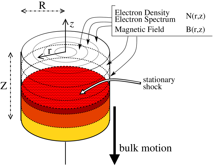
Figure 2: The geometry of the blob model. The volume is divided into different zones in $r$ and $z$ directions, each zone with its own electron distribution and magnetic field. We also schematically show the setup for the variability of the simulations presented here. The hatched layer represents the stationary shock (§2.6.1). The blob, simulation volume, is moving downward and crossing the shock front. Zones that crossed the shock at earlier times have had some time to radiate the newly injected energy and are plotted in lighter color shades.

2.2 Geometry

As illustrated in Fig. 2, the code is built with 2D cylindrical geometry, with symmetry in the azimuthal direction. The volume has radius $R$ and length $Z$, and it is divided evenly into zones in the radial and vertical directions ($r$ and $z$ coordinates, $n_{\mathrm{r}}$, $n_{\mathrm{z}}$). In all runs presented here $n_{\mathrm{r}}=9$ and $n_{\mathrm{z}}=30$. The number of zones sets the resolution of the simulation for what concerns spatial inhomogeneities in the physical properties, either as directly set up or because of their different evolution (e.g. radiation energy density will always develop a radial profile, in turn inducing a radial profile in the electron spectra). In the scheme adopted for this work the number of zones is also related to the duration of the Monte Carlo time-step (see § 2.3). For scenarios where the variability is produced by a perturbation crossing the simulation volume moving along the $z$ axis, spatial/temporal resolution in the $z$ direction is more important, hence we select a larger $n_{\mathrm{z}}$. For the simulations presented here our choice yields a Monte Carlo time resolution of $\Delta z/c/\delta\leq 500$ s in the observer’s frame, adequate to model the 2001 Mrk 421 data. It is possible to study faster variability, e.g. $<5$ minutes as observed in PKS 2155$-$304 (Aharonian et al., 2009), by increasing the number of zones at the expense of increased computational time. It is worth noting that as long as the choice of $n_{\mathrm{r}}$, $n_{\mathrm{z}}$ ensures that each zone is small enough to sample properly the variations on the physically relevant time-scales, the results of the simulations are substantially insensitive to these parameters.

This geometrical setup is adequate for the case we want to study since the assumption is that the active region is a slice of a collimated jet. In principle, the code setup is flexible enough that slightly different geometries could be simulated via the parameter settings in each zone.

Each zone has its own electron population (spectrum, density) and magnetic field. They can be setup individually and their time evolution is independent from each other, except for the effect of mutual illumination. Photons move freely among different zones, but the code assumes that electrons stay in their given zone and do not travel across zones; the electron Larmor radius is very small for the energies and (tangled) magnetic field strengths typical for the active region of a blazar jet, at least those studied here. For instance, for $\gamma=10^{6}$ and $B=0.03$ G, $r_{\mathrm{L}}=5.7\times 10^{10}$ cm, to be compared with source size of the order of $10^{16}$ cm. The radiation emitted by the blob is registered in the form of a pseudo-photon list (see §2.3.1), with time, direction and energy (see also Stern et al., 1995).

All the calculations are done in the blob rest frame. The transformation of all the quantities into the observer’s frame is performed afterwards. The output is analyzed using a separate post processing code to produce SEDs and light curves. Since the product of the code is effectively a photon list, we have significant freedom in the choices of bin sizes for time, energy, and angle, mostly limited by statistics, much in the same way as for actual observations. Hence, we can tailor the simulation results to the characteristic of the observations that we want to reproduce (e.g. time binning, energy bands).

In all cases presented here, the observed spectrum is obtained by integrating the beamed photons over a small solid angle centered around the angle $\theta$ between jet axis and observer, assumed as customarily to be $\theta=1/\Gamma$, for which also $\delta=\Gamma$. The typical width of the integration solid angle is $\Delta\cos(\theta)\sim\mathrm{few}\times 10^{-4}$.

2.3 The Monte Carlo section

The MC part of the code uses the current electron distribution, as updated in the F-P section of the code. It includes all processes that involves changes in the radiation field, such as Compton scattering and the production of new photons by various radiative processes, the most important of which for our case is synchrotron emission. Other notable processes are pair production and annihilation, and synchrotron self-absorption.

The MC time-step is currently a user-set parameter, part of a run input setup. It is adjusted depending on the geometry of the problem, e.g. shorter than the light crossing time of the smallest zone, and requirements of physical accuracy, for instance with respect to the fact that during each MC time-step the code does not change the electron distribution, which is evolved only during the F-P section of the code (i.e. ensuring that $\Delta t^{\prime}_{\mathrm{MC}}<\tau^{\prime}_{\mathrm{cool}}(\gamma)$ for the highest energy electrons.)

2.3.1 Monte Carlo particles

Since it is impossible to follow every individual photon a common technique used in radiative transfer problems is to group them into packets, pseudo-photons (e.g. Abbott & Lucy, 1985; Stern et al., 1995), to which we will refer as Monte Carlo particles. Every MC particle $k$ represents $n_{\mathrm{k}}$ photons with the same energy, the same velocity vector, at the same position and time, carrying a total energy of $E_{\mathrm{k}}=n_{\mathrm{k}}(\nu_{\mathrm{k}})\,h\nu_{\mathrm{k}}$. The $n_{\mathrm{k}}$ is also referred to as statistical weight of the MC particle.

The MC particles are born in the volume through emission processes, primarily synchrotron radiation in our case. The luminosity of the newly radiated synchrotron contribution is computed and converted into MC particles with a distribution according to the probability given by their SED.

The position within a given zone, time within the current time-step, and travel direction of the MC particle when it is generated are drawn randomly from the appropriate probability distributions.

At every time-step, each MC particle moves independently, with some probability of being IC scattered. Absorption is handled as a decrease of the statistical weight of the MC particles.

When a MC particle reaches the volume boundary, it is recorded with the full information of the escape time, position, direction, and energy, forming a list of emitted photons.

2.4 The Fokker–Planck equation

In each zone, the temporal evolution of the local electron population is obtained by solving the Fokker–Planck equation:

$$\begin{split}\frac{\partial N(\gamma,t)}{\partial t}&=-\frac{\partial}{\partial\gamma}\bigg{[}N(\gamma,t)\dot{\gamma}(\gamma,t)\bigg{]}\\ &+\frac{1}{2}\frac{\partial^{2}}{\partial\gamma^{2}}\bigg{[}N(\gamma,t)D(\gamma,t)\bigg{]}+Q(\gamma,t)-\frac{N(\gamma,t)}{t_{\mathrm{esc}}}\end{split}$$ (1)

$N(\gamma,t)$ is the electron spectrum, $\gamma$ is the random Lorentz factor of electrons, $\dot{\gamma}$ is the total heating/cooling rate. The IC cooling uses the time dependent radiation field calculated in the Monte Carlo part of the code, with LCTEs accounted for, which is considered constant for the duration of the F-P section of the code. The full Klein–Nishina (K-N) scattering cross section is used (see §2.6.3). $D(\gamma,t)$ is the dispersion coefficient which is not important for the type of scenarios presented in this work, and it then set to zero. For generality, the $D(\gamma,t)$ term is still included in the solving of the F-P equation. $Q(\gamma,t)$ is the electron injection term. Because, as noted in § 2.2, the electrons’ Larmor radius is much smaller than the size of the simulation zones, the particle escape term is not considered.

The time-step of the F-P loop is adjusted automatically depending on the rate of change (gain or loss) of energy of the particles to ensure a physically meaningful solution. It is constrained to be shorter than one fourth of the MC time-step.

Rather than using the discretization scheme proposed by Nayakshin & Melia (1998), as done in Böttcher et al. (2003), we choose to adopt the implicit difference scheme proposed by Chang & Cooper (1970). This scheme guarantees non-negative solutions, which in runs with the original scheme resulted in wild oscillations of the electron distribution at the high energy end (for a discussion of this issue please refer to the appendix of Chang & Cooper, 1970).

The energy grid used for the electrons is logarithmic in kinetic energy $x_{j}=\gamma_{j}-1$, with 200 mesh points from $x_{\mathrm{min}}=0.18$ to $x_{\mathrm{max}}=3.1\times 10^{7}$, i.e. $x_{j}=1.1\,x_{j-1}$.

After rewriting (1) as

$$\begin{split}\frac{\partial N(\gamma,t)}{\partial t}&=\frac{\partial}{\partial\gamma}\bigg{[}\bigg{(}-\dot{\gamma}(\gamma,t)+\frac{1}{2}\frac{\partial D(\gamma,t)}{\partial\gamma}\bigg{)}N(\gamma,t)\\ &+\frac{1}{2}D(\gamma,t)\frac{\partial N(\gamma,t)}{\partial\gamma}\bigg{]}+Q(\gamma,t)-\frac{N(\gamma,t)}{t_{\mathrm{esc}}}\end{split}$$ (2)

It is possible to discretize it as:

$$\begin{split}\frac{N_{j}^{n+1}-N_{j}^{n}}{\Delta t}&=\\ \frac{1}{\Delta x_{j}}&\Bigg{[}\frac{1}{\Delta x_{j+1/2}}C_{j+1/2}\ w_{j+1/2}\frac{1}{1-e^{-w_{j+1/2}}}N_{j+1}^{n+1}\\ -\,&\Bigg{(}\frac{1}{\Delta x_{j+1/2}}\ C_{j+1/2}\ W_{j+1/2}\ \\ +\,&\frac{1}{\Delta x_{j-1/2}}\ C_{j-1/2}\ w_{j-1/2}\ \frac{1}{1-e^{1-w_{j-1/2}}}\Bigg{)}N_{j}^{n+1}\\ +\,&\frac{1}{\Delta x_{j-1/2}}\ C_{j-1/2}\ W_{j-1/2}\ N_{j-1}^{n+1}\Bigg{]}\\ +\,&Q_{j}^{n+1}-\frac{1}{t_{\mathrm{esc}}}N^{n+1}_{j}\end{split}$$ (3)

with

$$B_{j+1/2}=-\frac{1}{2}\big{[}\dot{\gamma}_{j}+\dot{\gamma}_{j+1}\big{]}+\frac{D_{j+1}-D_{j}}{2\Delta x_{j+1/2}},$$

$$C_{j+1/2}=\frac{1}{4}(D_{j}+D_{j+1}),$$

$$w_{j+1/2}=\Delta x_{j+1/2}B_{j+1/2}/C_{j+1/2},$$

$$W_{j+1/2}=w_{j+1/2}/(\exp(w_{j+1/2})-1).$$

Here the $j\pm 1/2$ subscripts refer to quantities computed as the average values of the two adjacent grid points, such as

$$C_{j+1/2}=\frac{1}{2}(C_{j}+C_{j+1})$$

An exception is that of

$$\Delta x_{j}=\sqrt{\Delta x_{j+1/2}\Delta x_{j-1/2}}$$

with

$$\Delta x_{j+1/2}=x_{j+1}-x_{j}$$

$$\Delta x_{j-1/2}=x_{j}-x_{j-1}.$$

In order to avoid infinity in our calculation, we set $D=10^{-40}s^{-1}$ instead of $D=0$.

The tridiagonal matrix formed by equation (3) can be solved using the standard algorithm in Press et al. (1992).

2.5 Synchrotron and inverse Compton

The synchrotron spectrum is calculated adopting the single particle emissivity averaged over an isotropic distribution of pitch angles given by Crusius & Schlickeiser (1986) (Ghisellini et al., 1988):

$$\begin{split}P(\nu,\gamma)&=\\ \frac{3\sqrt{3}}{\pi}\,&\frac{\sigma_{\mathrm{T}}\,c\,U_{\mathrm{B}}}{\nu_{\mathrm{B}}}\,y^{2}\left\{K_{\frac{4}{3}}(y)K_{\frac{1}{3}}(y)-\frac{3}{5}\,y\left[K^{2}_{\frac{4}{3}}(y)-K^{2}_{\frac{1}{3}}(y)\right]\right\}\end{split}$$ (4)

where $\sigma_{\mathrm{T}}$ is the Thomson cross section and

$$\gamma=\frac{E}{m_{\mathrm{e}}c^{2}},\qquad\nu_{\mathrm{B}}=\frac{eB}{2\pi m_{\mathrm{e}}c},\qquad y=\frac{\nu}{3\gamma^{2}\nu_{\mathrm{B}}},$$

with $E$ the total electron energy, and $K_{x}(y)$ is the modified Bessel function of order $x$.

The total emitted synchrotron power and self-absorption coefficients are calculated according to the formulæ in Rybicki & Lightman (1979).

$$\alpha_{\nu}=\frac{c^{2}}{8\pi h\nu^{3}}\int dE\,P(\nu,E)\,E^{2}\,\left[\frac{N(E-h\nu)}{(E-h\nu)^{2}}-\frac{N(E)}{E^{2}}\right]$$ (5)

where $P(\nu,E)$ is the synchrotron spectrum given above (4).

For the total Compton cross section, we used the angle-averaged cross section given in Coppi & Blandford (1990):

$$\begin{split}\sigma(\omega,\gamma)&=\frac{3\sigma_{\mathrm{T}}}{32\gamma^{2}\beta\omega^{2}}\bigg{[}-\frac{x}{2}+\frac{1}{2(1+x)}+\\ &\bigg{(}9+x+\frac{8}{x}\bigg{)}\ln(1+x)+4Li_{2}(-x)\bigg{]}\Bigg{|}_{x=2\gamma(1-\beta)\omega}^{x=2\gamma(1+\beta)\omega}\end{split}$$ (6)

Where $Li_{2}(z)$ is the dilogarithm, which is evaluated numerically. To get the total cross section for a photon in an electron medium we need to integrate over $\gamma$, weighted by the electron energy distribution.

2.6 Other major changes

Besides changing the numerical scheme to solve the F-P equation, we implemented several other major changes in the code.

2.6.1 Injection of electrons

The model of the electron injection process, as implemented currently, involves a stationary shock perpendicular to the axis of the cylinder (jet) (Fig. 2). Hence, in the frame of the blob the shock is traveling across the blob with a speed equal to the bulk velocity of the blob $v_{\mathrm{bulk}}\sim c$. This scenario is similar to the one discussed by Chiaberge & Ghisellini (1999). The thickness of the shock is treated as negligible, in the sense that it is considered active only in one zone at any given time, i.e. it never splits across a zone boundary. However, during the time it takes to travel along a $Z$-zone, $\Delta z/c$, particles are injected in the entire zone volume. From this point of view the ‘shock’ thickness is not negligible. Provided that the $\Delta z$ of each zone is small this approximation is reasonable. As noted, for the cases presented here, $\Delta z/c/\delta\leq 500$ s. The total duration of injection is thus $t^{\prime}_{\mathrm{inj}}=Z/v_{\mathrm{bulk}}$, and each slice of the simulation volume along the $z$ axis will eventually have an injected energy of $L^{\prime}_{\mathrm{inj}}\Delta z/v_{\mathrm{bulk}}$, where $\Delta z=Z/n_{\mathrm{z}}$ is the thickness of one slice.

Electron injection is included in the Fokker–Planck equation through the term $Q(\gamma,t)$. The shock moves at the speed of $v_{\mathrm{bulk}}$ every F-P time-step. When the shock front is located in a given zone, electron injection is active ($Q\not=0$), otherwise $Q=0$. In the simulations presented here the injected electrons have a power law distribution with a high energy exponential cutoff

$$Q(\gamma)=Q_{0}\,\left(\frac{\gamma}{\gamma_{0}}\right)^{-p}\,\mathrm{e}^{-\gamma/\gamma_{\mathrm{max}}}\hfill\text{cm}^{-3}\,\text{s}^{-1}\hfill\gamma\geq\gamma_{\mathrm{min}},$$

The value of the normalization $Q_{0}$ is controlled by the parameter $L^{\prime}_{\mathrm{inj}}$.

Injection and acceleration time-scales and durations are in principle independent from other parameters and could be set directly on the basis of a hypothesis on the details of physical processes underlying them. In this work we are treating injection, and in turn the implied process for accelerating the newly injected particles, phenomenologically, affording ourselves the freedom to assume their spectrum and time-scales.

The underlying physical mechanism for the injection process is not specified. First order Fermi acceleration at a shock front or second order Fermi acceleration by a plasma turbulence are two possible processes (e.g. Drury, 1983; Blandford & Eichler, 1987; Gaisser, 1991; Protheroe, 1996; Kirk et al., 1998; Katarzyński et al., 2006).

2.6.2 Splitting of MC particles

A major difficulty of using the Monte Carlo method to model broadband IC emission, in the physical conditions typical of blazar jets, is the low pseudo-photon statistics at high frequencies. Observations are affected by a very similar problem.

Blazar SEDs are approximately flat in ($\nu F_{\nu}$) over wide range of energies. In blue blazars typical energies for the electrons responsible for the ($\nu F_{\nu}$) emission peaks, occurring in UV-X-ray and TeV bands, are $\gamma\sim 10^{4}-10^{5}$. When a photon (for us a MC particle) is scattered to the TeV range, the energy of that MC particle will increase by about 9–11 orders of magnitude depending on whether it was an X-ray or optical photon, and its ‘flux’ will decrease by the same factor, making the statistics of the high energy IC component very poor.

An additional challenge that we face is that the IC scattering probability is very small. Under most reasonable conditions the active blob is very optically thin.

In order to mitigate these problems, we introduced a method relying on the splitting of MC particles. The basic idea is that since every MC particle represents a packet of real photons treated together, it is always possible to divide them into smaller packets. If this splitting is applied in appropriate conditions, it is possible to achieve a reasonable statistics on MC particles at high frequencies with reasonable computer resources.

We have implemented MC particle splitting in three different instances within the context of the computation of IC scattering.

1. The first splitting is applied to every MC particle when it is considered for IC scattering. It is split into a large number of identical subparticles (e.g. $\sim 10^{3}$). The choice of this number depends on the trade off between improving the statistics of the high energy photon spectrum and cost in terms of computing resources (time and memory), and it was based on empirical testing. Whether a particle is scattered or not is determined by comparing the distance it would travel with a distance to the next scattering stochastically determined from its mean free path. Every MC subparticle draws a separate random number, and in turn has its own probability of being scattered. All non-scattered MC subparticles are recombined into a MC particle, and travel to a new position. The subparticles that do scatter (usually a small number) will be scattered separately, to independent energies and directions (but see below). This first splitting does not necessarily save a computational time, but it decreases dramatically the memory allocation requirement to achieve the desired statistics at the highest SED energies.

2. The second instance of splitting is applied to MC (sub)particles that are being scattered. They are divided into another large number (e.g. $\sim 10^{3}$), and each of these MC sub-subparticles will be scattered separately, to a frequency and direction uncorrelated with those of the other particles. This splitting allows us to concentrate computation cycles on the rare events of scatterings, which is what we are most interested in.

3. Even with this second splitting, at highest energies the statistics of the IC photon spectrum remains very poor. To alleviate this problem, we implemented a third instance of MC particle splitting. It is triggered when one of the already twice-split MC particles is scattered to very high frequency, above a threshold that is set a priori and constant for each run, tailored to the characteristics of the studied SED. This MC particle is split again, and each of its subparticles is re-scattered from the original frequency. That scattering is accepted only when the scattered frequency is higher than the preset threshold, otherwise it goes back and draws another random number. This third splitting offers the benefit of avoiding the use of a much larger number of subparticles in the second instance of splitting, and subsequently avoiding the production of a very large number of MC particles to be recorded in the computer memory.

Splitting causes the number of MC particles to grow during the simulation. Nevertheless, the advantage over directly setting up the simulation with more MC particles is significant both in terms of number of MC particles and more importantly because the new MC particles are created where they are most needed, thus increasing greatly the efficiency of the code. In typical runs the increase in the number of MC particles due to the splitting is modest, of the order of 10–20 per cent of the number of newly emitted synchrotron photons at each MC step.

2.6.3 Arbitrary electron energy distribution

Although the F-P equation can calculate the time dependent evolution of the electrons with arbitrary spectrum, earlier versions of the code forced the decomposition of the electron population into a low-energy thermal population plus a high-energy power law tail. The emissivity of cyclotron, non-thermal synchrotron and thermal bremsstrahlung radiation processes were calculated on the basis of this decomposition. The calculations of the synchrotron self-absorption coefficient and the total scattering cross section of a photon in the medium were dependent on this ‘thermal plus power law’ approximation as well. In order to make the code more general, and in particular more suitable for blazar simulations, in which there is usually a dominant non-thermal lepton population, we have entirely rewritten the relevant sections of the code. The code now calculates all physical quantities using the actual electron spectrum, as updated by solving the F-P equation (see § 2.5)

2.7 Deactivated Features

Some features of the code have been deactivated in this study. Among these are the cyclotron and bremsstrahlung emission and Coulomb scattering of electrons with protons, all considered not important in blazar jets. Others are turned off because they are not the focus of this paper; these include external sources of photons, which will be subject of future investigations.

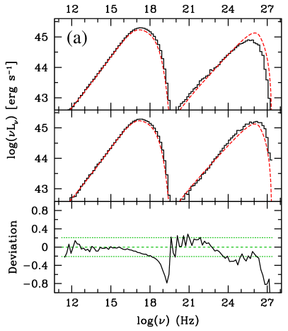
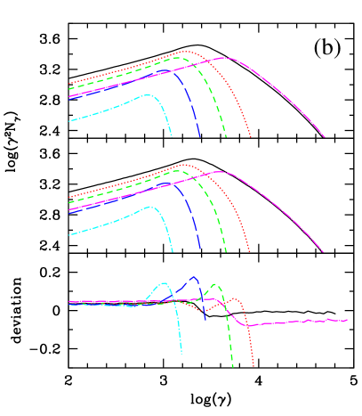
Figure 3: (a) Results of the steady state homogeneous model simulation. The smooth red lines are the SEDs from Fossati et al. (2008). The black histogram is the SED produced by our MC/F-P model run with the closest possible source setup. In the top panel we used the full K-N cross section, while in the middle we used a step function approximation as done in Fossati et al. (2008). The bottom panel shows the fractional deviation, $\Delta y/\langle y\rangle$, between these two latter SEDs. Positive sign corresponds to the one-zone spectrum having a larger value. (b) Results of the time-dependent homogeneous model simulation. Electron distributions, as $\gamma^{2}N(\gamma)$, for different times for our MC/F-P code (top), or the one-zone code of Chiaberge & Ghisellini (1999) (middle). In different colors and line types we plot the spectra at the following times (in units of $R/c$): 0.5 (magenta, long dash dot), 1 (black, solid), 1.25 (red, dotted), 1.5 (green, sort dash), 2 (blue, long dash), 3 (cyan, dot dash). In the bottom panel we show the fractional deviation, $\Delta y/\langle y\rangle$, between the spectra for the two codes. Lines are truncated at the energy where $\gamma^{2}N_{\gamma}$ drops a factor of 30 below its peak value.

3 Test Runs

In order to test the reliability and robustness of the code, we compared the results of our code with those of other authors using different codes, for cases where the codes’ capabilities are comparable. We first compare the results with a non time-dependent code to test the MC radiative part of the code. Then we compare the electron evolution with a time dependent code, in a single-zone homogeneous case. Generally the results match very well.

3.1 Steady state SED of homogeneous models

To test how the code handles the radiative processes, we try to reproduce the theoretical SED shown in Fossati et al. (2008), for the non-extreme parameter choice (solid line in their fig. 10a). That SED was computed with a single-zone homogeneous SSC model. The electrons are assumed to be continuously injected and reach a steady state (e.g. Ghisellini et al., 1998). For this test, we take the equilibrium electron distribution calculated in the homogeneous code as our input electron distribution, and turn off the F-P evolution of the electrons. We cut the volume into several identical zones just to make use of the parallel structure of the code. Since the single-zone model uses a spherical geometry, while our MC model uses a cylindrical geometry, we choose to use the same radius ($R=10^{16}$ cm), but with the height of the cylinder $Z=4/3R$, in order for the two models to have the same volume. The produced SED is shown in Fig. 3a in the top panel as black histogram, directly compared with that of Fossati et al. (2008). In general the two SEDs match well, except for a slight discrepancy around the peak of the IC component. This arises from the fact that the single zone model uses a step function to approximate the K-N cross section, while our code implements the full K-N cross section.

We then also tested our code with the step function approximation. The result in shown in Fig. 3a, middle panel. The overall shapes of the SEDs match better. The total luminosity seems a little higher in the MC model. However, it is worth noting that although we are matching the volume, the geometry is different in the two codes and this has a small effect on the IC component. Moreover, in order to achieve a reasonable statistics the emitted photons are integrated over a finite solid angle, i.e. a range of angles $\theta$ (photon direction angle with respect to the jet axis, in the observer frame). Hence for a given bulk Lorentz factor $\Gamma_{\mathrm{bulk}}=26$, we are effectively integrating over a range of Doppler factors $\delta\simeq 23.5\sim 28.7$, not exactly $\delta=26$ as for the comparison model.

3.2 Temporal evolution (one zone model)

The other important aspect of our MC/F-P code, the Fokker–Planck evolution of the electrons, was tested by comparing the code with the one-zone time dependent homogeneous SSC code by Chiaberge & Ghisellini (1999). We set the number of zones to one, and used a power law injection with the same parameters they used ($B=1$ G, $\gamma_{\mathrm{min}}=1$, $\gamma_{\mathrm{max}}=10^{5}$, $p=1.7$, $L^{\prime}_{\mathrm{inj}}=3.69\times 10^{41}$ erg/s, $t^{\prime}_{\mathrm{esc}}=1.5R/c$, $t^{\prime}_{\mathrm{inj}}=R/c$), except that our geometry is a cylinder with $R=1.1547\times 10^{16}$ cm, $Z=10^{16}$ cm, while they use a sphere with $R=10^{16}$cm.

The electron spectra at different times are shown in Fig. 3b; the upper panel shows the one produced by the MC code, the middle panel the one produced by the one-zone code, while the bottom panel shows the deviation. The two spectra match reasonably well, giving us confidence that our code handles the evolution of the electron distribution correctly.

4 Application to Mrk 421

Mrk 421 is the archetypical ‘blue’ blazar, the most luminous and best monitored object in the UV, X-ray and TeV bands. It was the first extragalactic source detected at TeV energies (Punch et al., 1992). As such it has been the target of multiple multiwavelength campaigns with excellent simultaneous coverage by X-ray and TeV telescopes. (Takahashi et al., 2000; Maraschi et al., 1999; Fossati et al., 2000a, b; Krawczynski et al., 2001; Błażejowski et al., 2005; Rebillot et al., 2006; Giebels et al., 2007; Fossati et al., 2008; Donnarumma et al., 2009).

For a first application of our code we focused on one of best flares ever observed, occurred on 2001 March 19 (Fossati et al., 2008). It was a well defined, isolated, outburst that was observed both in the X-ray and $\gamma$-ray bands from its onset through its peak and decay. It uniquely comprised several rare favorable features, namely absence of data gaps (except RossiXTE’s short orbital gaps), excellent TeV coverage by the HEGRA and Whipple telescopes and large amplitude variation in both X-ray and $\gamma$-ray bands.

4.1 Observational constraints and goals

We aim to reproduce several observational features. Some of them can be regarded as constraints on the setup of a baseline model, as they provide guidance on the general properties and parameter values yielding an acceptable fit to the SEDs (e.g. Tavecchio et al., 1998, Bednarek & Protheroe, 1997, and Fossati et al., 2008 for an example specific for the observations studied here). In this respect, we have five fundamental observables we want to match:

• The peak frequencies of the synchrotron and IC components, $\nu_{\mathrm{p,S}}$, $\nu_{\mathrm{p,IC}}$, which for Mrk 421 are observed in the X-ray and $\gamma$-ray bands.

• The peak luminosity and the relative strengths of the two SED components, $\nu L_{\mathrm{p,S}}$, $\nu L_{\mathrm{p,IC}}$.

• The variability timescale ($t_{\mathrm{var}}$). Combined with an hypothesis on the Doppler factor it provides a constraint on the size of the blob. For Mrk 421 in X-ray and $\gamma$-ray it is typically of the order of tens of kiloseconds.

Besides giving an indication about the size of the active region, the latter can be different for different energy bands and in turn its energy dependence can provide additional constraints on the model parameters and source geometry.

There is then a set of observational features whose explanation remains to a large extent an open question. They represent the ultimate goal of our work and the driver for the development of a time dependent multi-zone model.

1. The quasi-symmetry of flare light curves, showing similar rising and falling time-scales, both in X-rays and $\gamma$-rays. The symmetry seems to be a quite common feature at several wavelengths. It would seem to support the interpretation that the flare evolution is governed by the geometry of the active region (Chiaberge & Ghisellini, 1999; Kataoka et al., 2000). However, this could be true only if all other (energy dependent) time-scales are shorter than the blob crossing time, or relevant geometric time-scale, or only for emission at energies for which this is true.

2. The characteristics of the multiwavelength correlated intensity variations. The flare amplitude is generally larger in $\gamma$-rays than in the X-ray band, and flux variations show a quadratic (or higher order) relationship that holds during both the rise and the decay phases of the flare. This behavior was observed in Mrk 421 on 2001 March 19, and also for other ‘clean’ flares, including for other blue blazars (e.g. Aharonian et al., 2009, reporting a cubic variation for PKS 2155$-$304).

3. The existence and length of inter-band (X-ray vs. $\gamma$-ray) and intra-band (soft X-ray vs. hard X-ray) time lags, often with changing sign from flare to flare (see references given above for Mrk 421). In the isolated flare of 2001 March 19, Fossati et al. (2008) report a possible lag of about 2 kilo-seconds of the TeV flux with respect to a soft X-ray band (2–4 keV), whereas TeV and harder X-rays (9–15 keV) were consistent with no lag. In turn an X-ray intraband lag was detected.

4. The fact that even during large outbursts the optical flux changes little. This may constrain the characteristics of the particle injection, such as their spectrum (shape and density) and energy span. On the other hand, the time dependent spectral behavior of blazars has led people to speculate that there is more than one component contributing to the blazar emission (Fossati et al., 2000b; Krawczynski et al., 2004; Błażejowski et al., 2005; Ushio et al., 2009). It is not clear if this additional zone is co-spatial with the zone undergoing the flare or it is far enough elsewhere along the jet that the two do not interfere with each other and evolve independently.

5. SED shape, and its time variations, particularly around the two peaks. For Mrk 421 we mostly focus on the X-ray and TeV $\gamma$-ray spectra.

These features have been observed in several instances for Mrk 421, mostly cleanly in the case of the 2001 March 19 flare, and the other well studied TeV detected blue blazars. For the brightest blue blazars there is an extensive database of multiwavelength observations and studies of time resolved spectral variability. The phenomenology is richer and more complex than the few items just introduced, on which we focus. In this respect, one of the most interesting findings is the observation of a correlation between luminosity and position of the peak of the synchrotron component (e.g. Tavecchio et al., 2001; Fossati et al., 2000b; Tanihata et al., 2004; Tramacere et al., 2007).

In this work we are mostly aiming at illustrating the capabilities of our code with respect to investigating the above observational findings, by presenting the results of simulations of three simple scenarios.

Table 1: Summary of model parameters

Case		general source parameters					back-/fore-ground component					injected component
		$R$	$Z$	$\Gamma$	$B$		$\gamma_{\mathrm{min}}$	$\gamma_{\mathrm{b}}$	$\gamma_{\mathrm{max}}$	$n_{\mathrm{e}}$		$\gamma_{\mathrm{min}}$	$\gamma_{\mathrm{max}}$	$L^{\prime}_{\mathrm{inj}}$
		$10^{16}$	$10^{16}$											$10^{40}$
		cm	cm		G					cm-3				erg s-1
1: with ‘background’		1.0	1.33	33	0.1		50	$2\times 10^{4}$	$2\times 10^{5}$	4.0		$50$	$1.9\times 10^{5}$	5.5
2: with ‘foreground’		1.0	1.33	33	0.08		50	$1\times 10^{4}$	$1\times 10^{5}$	6.0		$50$	$1.9\times 10^{5}$	6.0
3: better TeV spectrum		1.5	2.0	46	0.035		50	$2\times 10^{4}$	$2\times 10^{5}$	1.56		$50$	$1.9\times 10^{5}$	3.2

All background or foreground components electron spectra are broken power laws (with exponential cutoff), with spectral indices $p_{1}=1.5$, $p_{2}=2.5$ ($=p_{1}+1$). The injected power law has spectral index $p=1.5$ in all cases.

4.2 On model parameters

This code affords us a great freedom. In particular, we could setup each zone with different initial conditions. However, for the scenarios presented in this work we took a conservative approach and setup each zone with identical values for the usual set of physical parameters.

Our homogeneous (at least initially) SSC model is defined by the following quantities (see also Table 1):

• source size/geometry ($R$, $Z$, or aspect ratio),

• Lorentz factor ($\Gamma$),

• magnetic field strength ($B$),

• various parameters describing the electron spectrum, e.g. four for an injected power law: $\gamma_{\mathrm{min}}$, $\gamma_{\mathrm{max}}$, $p$, $L^{\prime}_{\mathrm{inj}}$. For a broken power they would be six because there would be a spectral break $\gamma_{\mathrm{b}}$ and two spectral indices ($p_{1}$, $p_{2}$) instead of one.

With simple considerations we can reduce the number of model parameters to constrain from 8 (or 10) to 5 ($B$, $\Gamma$, $R$, $\gamma_{\mathrm{max}}$, $L^{\prime}_{\mathrm{inj}}$) and as illustrated in the previous section we have $5+$ fundamental observables to do it.

The source aspect ratio can be at least qualitatively constrained by the profile of the flare light curve, for in first approximation extreme geometries would yield fairly distinctive flare shapes due to LCTE. For this work we adopted a conservative, stocky, volume aspect ratio $R/Z=3/4$, i.e. width:length = 3:2.

Among the electron spectrum parameters, $\gamma_{\mathrm{min}}$ and $p$ (or $p_{1}$) can be set with reasonable confidence based on considerations on the SED shape and variability (or lack thereof) at frequencies below the synchrotron peak. The precise value of $\gamma_{\mathrm{min}}$ is however not well constrained by observations. The emission by electrons at $\gamma\leq 10^{3}$ would be below the optical band, where there is not much simultaneous coverage, and emission by much lower energy electrons would fall in a band (i.e. $\nu\leq 10^{11}$ Hz) where observations suggest that the SED is dominated by radiation from other regions of the jet (e.g. Kellermann & Pauliny-Toth, 1981). Moreover, cooling time-scales for electrons at those energies are long compared with the typical duration high-density multiwavelength campaigns (see eq. 11), making it difficult to set a constraint on $\gamma_{\mathrm{min}}$ based on variability. Higher values of $\gamma_{\mathrm{min}}$ affect the synchrotron emission in the optical band and in turn the IC component, mainly in the GeV band, and therefore we can assess their viability with current and future observations. Given that during the 2001 campaign (Fossati et al., 2008) there seemed to be a modest level of variability in the optical band, $\Delta m_{\mathrm{V}}\simeq 0.4$, though not directly from observations simultaneous with the March 19 flare, we simulated scenarios where the injected electron population has a relatively low $\gamma_{\mathrm{min}}=50$ (Table 1). We choose to truncate the electron distribution at this value also because the number of low energy electrons grows rapidly, thus increasing significantly the computational time without adding much to the investigation presented here; as noted, emission from lower energy electrons would not be detectable, and they would not significantly alter the properties of the emission and its variability observed in blue blazars. This is of course an assumption that is valid for this work but that should be revisited, for instance for the study of red blazars.

The spectral indices of the injected electron distributions $p$ or $p_{1}$ ($p_{2}=p_{1}+1$ as expected for a cooling break) are mostly constrained by the shape of the synchrotron SED at energies below the optical range. The preferred value for $p,p_{1}=1.5$ constitutes a somewhat hard spectrum but it is consistent with values discussed by several particle acceleration studies. In particular, stochastic (2^nd-order Fermi acceleration) and acceleration at relativistic shear layers have been suggested to produce very hard ($p<2$) particle spectra (Virtanen & Vainio, 2005; Stawarz & Ostrowski, 2002; Rieger & Duffy, 2004, 2006).

In the context of this discussion, it is worth adding that we considered scenarios with and without a pre-existing population of relativistic electrons or an external ‘diluting’ SED (see § 4.4 and § 4.5 for details), and their characteristics could be regarded as an additional degree of freedom of our modeling. In this respect, however, while a particular choice of values has some effect on the best parameters for the component responsible for the variability, its effect is fairly limited and the most important point is the existence or not of such secondary component (see § 5).

Next, we illustrate some general arguments and estimates for values of the fundamental physical parameters. We then present and discuss the results obtained with the set of parameters that we deemed more successful, and in turn ‘fit’ the SEDs and light curves of the 2001 March 19 outburst testing several different parameter combinations, including the possible dilution by emission from a different region of the jet not involved in the flare, and the presence of a pre-existing electron population in the region that becomes active.

4.3 Estimates of active region parameters from observables

Key parameters in the modeling of blazars with the SSC model include the Lorentz factor, the magnetic field strength, the size of the volume, and the energy of the electrons that are responsible for the synchrotron peak of the SED, $\gamma_{\mathrm{p}}$. This latter is associated with a break in the electron distribution or its maximum, depending on the spectral index. We use the observational results of Fossati et al. (2008) as the benchmark of our analysis. There are several observed features that constrain the value of these parameters (see previous section). Additionally, independent estimates of the relativistic beaming parameters of blazars, from observed superluminal motion as well population statistics, yield Lorentz factors of the order of tens (Urry & Padovani, 1995). As we mentioned before, we make the common assumption to be observing the source at the angle $\theta=1/\Gamma$, hence $\delta=\Gamma$ (see Cohen et al., 2007, for a deeper statistical analysis, showing that the most likely combination is $\Gamma\sin\theta\simeq 0.7$).

The observed peak of the synchrotron component (at energy $E_{\mathrm{p,S}}$) results from the combination of electrons’ $\gamma$, $B$ and $\delta$. Assuming mono-energetic emission the relationship is $E_{\mathrm{p,S}}=\nu_{\mathrm{B}}\,\gamma^{2}_{\mathrm{p}}\,\delta$. For Mrk 421 $E_{\mathrm{p,S}}\simeq 1$ keV. Parameterized on fiducial values for these three parameters the $\gamma_{\mathrm{p}}$ of the electrons emitting at the synchrotron peak is:

$$\gamma_{\mathrm{p}}\simeq 1.7\times 10^{5}\;\left(\frac{B}{0.1\ \mathrm{G}}\right)^{\!\!-1/2}\left(\frac{\delta}{30}\right)^{\!\!-1/2}\left(\frac{E_{\mathrm{p,S}}}{1\ \mathrm{keV}}\right)^{\!\!1/2}$$ (7)

If the IC component peak resulted from scattering of photons of the synchrotron peak in Thomson regime we could directly infer the energy of the electrons emitting at both SED peaks as

$$\gamma_{\mathrm{p}}\simeq\left(\frac{3\,E_{\mathrm{p,IC}}}{4\,E_{\mathrm{p,S}}}\right)^{\!\!1/2}\!\!\simeq 2.7\times 10^{4}\left(\frac{E_{\mathrm{p,IC}}}{1\ \mathrm{TeV}}\right)^{\!\!1/2}\left(\frac{E_{\mathrm{p,S}}}{1\ \mathrm{keV}}\right)^{\!\!-1/2}$$ (8)

with $E_{\mathrm{p,IC}}$ is the peak energy of the IC component. However, as discussed by Fossati et al. (2008, see Fig. 11 therein), the SED shape and variability time-scale observed in Mrk 421 in 2001 favor parameters such that the scattering between electrons at $\gamma_{\mathrm{p}}$ and synchrotron peak photons at $E_{\mathrm{p,S}}$ would happen in the K-N regime (see also Tavecchio et al., 1998; Bednarek & Protheroe, 1999). In this case the IC peak energy would be largely independent of $E_{\mathrm{p,S}}$ and the expression would instead be:

$$\gamma_{\mathrm{p}}\simeq\frac{E_{\mathrm{p,IC}}}{\delta\,m_{\mathrm{e}}c^{2}}\;\simeq\;6.5\times 10^{4}\left(\frac{E_{\mathrm{p,IC}}}{1\ \mathrm{TeV}}\right)\,\left(\frac{\delta}{30}\right)^{\!\!-1}\,.$$ (9)

Requiring that the condition for Thomson regime, $\gamma x^{\prime}\leq 3/4$ (where $x^{\prime}=E^{\prime}_{\mathrm{target}}/(m_{\mathrm{e}}c^{2})$), holds true for $E^{\prime}_{\mathrm{target}}=E^{\prime}_{\mathrm{p,S}}$ and $\gamma=\gamma_{\mathrm{p}}$, one can derive a rough estimate of what ($B$, $\delta$) combination would be necessary to push into the Thomson regime the scattering between $\gamma_{\mathrm{p}}$ and its own synchrotron photons, emitted at $E_{\mathrm{p,S}}$.

$$\left(\frac{B}{0.1\ \mathrm{G}}\right)\left(\frac{\delta}{30}\right)^{\!\!3}\geq 220\,\mathbf{\left(\frac{E_{\mathrm{p,S}}}{1\ \mathrm{keV}}\right)^{\!\!3}}$$ (10)

As shown by Fossati et al. (2008), it is indeed possible to achieve an acceptable SED fit with high $B$ and $\delta$. However, while this kind of model matches equally well a static SED, its smaller blob size and extreme Lorentz contraction make it implausible when compared with more dynamic observational findings, beginning with the variability time-scales.

The rest frame synchrotron cooling time can be expressed as function of electron energy and the magnetic field:

$$\tau^{\prime}_{\mathrm{cool,S}}=\frac{7.7\times 10^{8}}{\gamma B^{2}}~{}~{}\mathrm{s}$$ (11)

or, more directly related to observables, in terms of observed photon energies:

$$\tau^{\prime}_{\mathrm{cool,S}}=4.6\!\times\!10^{5}\,\left(\frac{B}{0.1\ \mathrm{G}}\right)^{\!\!-3/2}\left(\frac{\delta}{30}\right)^{\!\!1/2}\left(\frac{E_{\mathrm{S}}}{1\ \mathrm{keV}}\right)^{\!\!-1/2}~{}\mathrm{s}$$ (12)

or, in the observer’s frame,

$$\tau_{\mathrm{cool,S}}=15.1\,\left(\frac{B}{0.1\ \mathrm{G}}\right)^{\!\!-3/2}\left(\frac{\delta}{30}\right)^{\!\!1/2}\left(\frac{E_{\mathrm{S}}}{1\ \mathrm{keV}}\right)^{\!\!-1/2}~{}\mathrm{ks}$$ (13)

showing its dependence on the inverse square root of the energy of the observed photons.

A general constraint among the observed variability time-scale and source size and time-scale of the acceleration, injection or cooling process is:

$$t_{\mathrm{var}}\geq\frac{1}{\delta}\,\max\left(\tau^{\prime}_{\mathrm{cool}},\tau^{\prime}_{\mathrm{acc}},t^{\prime}_{\mathrm{inj}},\frac{R}{c},\frac{Z}{c}\right)$$ (14)

As noted in Section 2.6.1, in this work we take a simplified approach, whereby we do not specify the acceleration mechanisms underlying the particle injection, and we choose to link the injection time-scale to the geometry of the source, namely its dimension along the jet axis, $Z$. Hence we have a simplified relationship with the observed variability, and considering that the 2001 March 19 flare has a flux doubling and halving time of the order of $10^{4}$ s, we have approximately

$$\max\left(\tau^{\prime}_{\mathrm{cool}},\frac{R}{c},\frac{Z}{c}\right)\simeq\max\left(\tau^{\prime}_{\mathrm{cool}},\frac{R}{c}\right)\simeq 10^{4}\,\delta\quad\mathrm{s}$$ (15)

Please note that this constraint could actually vary with the observed band because some time-scales are likely to be energy dependent.

If the IC cooling rate is similar to the synchrotron cooling rate $\tau^{\prime}_{\mathrm{cool}}\sim\tau^{\prime}_{\mathrm{cool,S}}/2$. The condition $\tau^{\prime}_{\mathrm{cool}}<R/c$ translates into

$$E_{\mathrm{S}}>0.46\;\left(\frac{R}{10^{16}\ \mathrm{cm}}\right)^{\!\!-2}\,\left(\frac{B}{0.1\ \mathrm{G}}\right)^{\!\!-3}\,\left(\frac{\delta}{30}\right)\quad\mathrm{keV}$$ (16)

From the constraints and relationships illustrated above we infer that a good starting point to model the SED of Mrk 421 is a combination of $R\sim 10^{16}$  cm, $B\sim 0.1$  G, $\Gamma\simeq\delta\sim 30$, $\gamma_{\mathrm{p}}\sim 10^{5}$.

Because of computational limitations we did not perform an actual fit to identify the best set of parameters values reproducing the SED and the flare evolution properties. We explored a limited range of values for $R$, $B$, $\Gamma$ around the values obtained from the above analysis, and focused on changes of the maximum electron energy $\gamma_{\mathrm{max}}$ and the injected power $L^{\prime}_{\mathrm{inj}}$.

We ran a large number of short simulations aimed at sampling a reasonable range of values around our initial guesses and evaluated them mostly on the basis of their matching the X-ray spectra and variability. In a second stage we honed in on the best cases and adjusted the parameters by means of full length simulations.

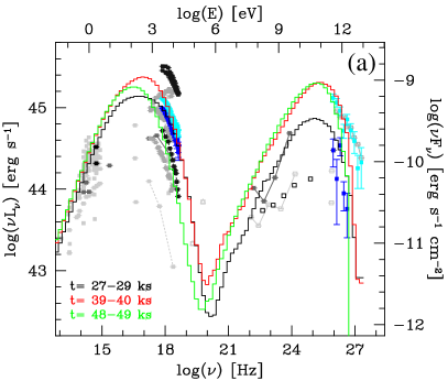
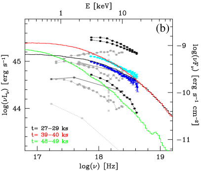
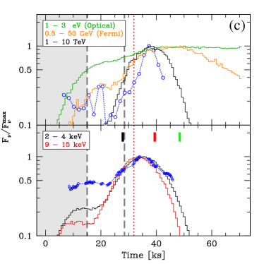
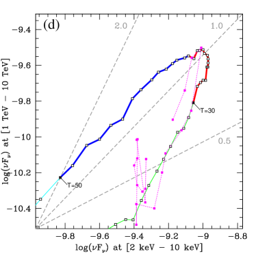
Figure 4: Summary of results of the first case, with pre-existing background electron population. All quoted times are in the observer’s frame. (a) Broad band SEDs for three representative times (see labels) during the simulation of the flare. Observed spectra for high and low states during the 2001 March 19 flare in X-ray and TeV $\gamma$-rays are plotted in cyan and blue. Other historical data points in grey or black are the same as in Fossati et al. (2008). The black empty squares in the GeV $\gamma$-ray band are the Fermi/LAT 1-year averages in five bands. (b) Zoom centered on the X-ray band. (c) Light curves at 5 different energy bands, on 700 seconds bins. Light curves are normalized to their peak values. In the bottom panel we show two X-ray energy bands, and in blue the RossiXTE/PCA 2–4 keV data. The top panel comprises the simulated TeV band light curve, to be compared with the blue data points, as well as light curves in optical and a band representative of the Fermi/LAT bandpass. The grey shaded area is intended to highlight the initial section of the light curve which is not meaningful because it corresponds to the interval during which the pre-existing electron population is being ‘prepared’. The long dashed vertical grey lines mark the injection period. The dotted red line marks the time corresponding to the largest cross-section of the active region along planes of equal observed times (see text, § 4.7). The colored short thick segments mark the times corresponding to the SEDs plotted in (a) and (b). (d) The flux vs. flux plot for X-ray and $\gamma$-rays. Simulations data have been smoothed with a one-hour width boxcar filter. Colors highlight different 10 ks time intervals. As labeled, red starts at t=30 ks. For the red and blue lines we used a thicker trait to highlight the central time interval of the outburst. The magenta points connected by a dotted line show the observed correlation of TeV flux in Crab units vs. X-ray in count rate for the 2001 March 19 flare. Because of the different units they are plotted at an arbitrary position.

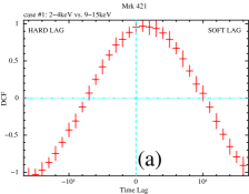
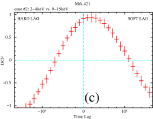
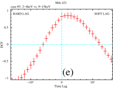
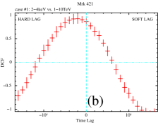
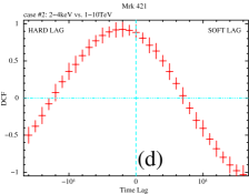
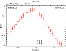
Figure 5: Discrete cross correlations analysis. Our simulated cases run left to right, (a, b) for the ‘background’ case, (c, d) for the ‘foreground’ case, (e, f) for the ‘better TeV spectrum’ case. Top panels show the intra-band X-ray correlation between X-ray ($2-4$ keV) and X-ray ($9-15$ keV), and bottom panels the inter-band correlation between soft(er) X-ray ($2-4$ keV) and TeV $\gamma$-rays.

4.4 Case 1: injection in a blob with a pre-existing (background) electron population

In all cases presented in this paper, the outburst is attributed to the injection into our active volume of a new population of higher energy electrons, with fixed injected spectrum (power law with exponential cutoff).

In this first scenario the blob is not empty, but it is filled with a ‘background’ population of electrons, homogeneous throughout the volume. These electrons serve as a slowly evolving component in the electron distribution and in turn the SED, which can be regarded as the remnants of a previous phase of activity. They participate fully in the time evolution of the blob, cooling and emitting radiation.

The overall best case has the following parameters: $R=10^{16}$ cm, $Z=4/3\times 10^{16}$ cm, $B=0.1$ G, $\Gamma=33$. Parameters for this and all following cases are summarized in Table 1.

At $t=0$ the electron spectrum for the ‘background’ population is a broken power law distribution:

$$N(\gamma) =N_{\mathrm{b}}\left(\frac{\gamma}{\gamma_{\mathrm{b}}}\right)^{-p_{1}} \text{cm}^{-3} \gamma_{\mathrm{min}}<\gamma<\gamma_{\mathrm{b}}$$

$$N(\gamma) =N_{\mathrm{b}}\left(\frac{\gamma}{\gamma_{\mathrm{b}}}\right)^{-p_{2}}\,e^{-\gamma/\gamma_{\mathrm{max}}} \text{cm}^{-3} \gamma_{\mathrm{b}}\leq\gamma$$

The spectral indices are $p_{1}=1.5$ and $p_{2}=2.5$. The break is at $\gamma_{\mathrm{b}}=2\times 10^{4}$, the high-energy cut-off at $\gamma_{\mathrm{max}}=2\times 10^{5}$. The number density of this ‘background’ population is $n_{\mathrm{e}}=4$ cm^-3. Their total energy content is $2.2\times 10^{46}$ ergs.

By the time when the new flare begins, i.e. the shock begins to cross the region and inject electrons, this pre-existing population has cooled to a $\gamma_{\mathrm{max}}$ of a few times $10^{4}$, yielding a synchrotron peak at around 50 eV. In the observer’s frame, the cooling time-scale for the peak of the ‘background’ component is of the order of 1 day and we could think of it as due to the aging of the electron spectrum from a previous active phase occurred a few days earlier. In most recent long observing campaigns Mrk 421 exhibited flares on about this time-scale (e.g. Takahashi et al., 2000).

The injection of electrons begins at $t^{\prime}_{\mathrm{start,inj}}=5\times 10^{5}$ s, with a power law distribution (§2.6.1). The parameters of the injected spectrum are: $p=1.5$, $\gamma_{\mathrm{min}}=50$, $\gamma_{\mathrm{max}}=1.9\times 10^{5}$, $L^{\prime}_{\mathrm{inj}}=5.5\times 10^{40}$ erg/s.

The emitted –beamed– photons are integrated over the angle of $0.99944<\cos(\theta)<0.99964$, which corresponds to a Doppler factor of $27<\delta<42$.

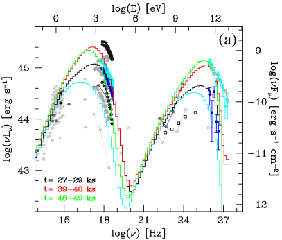
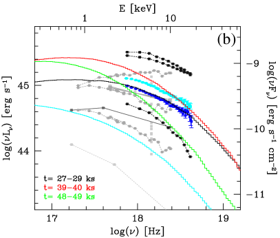
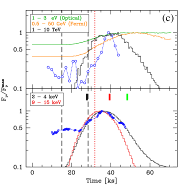
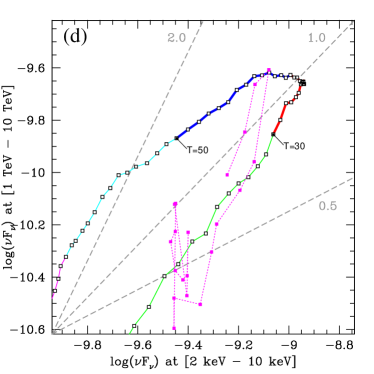
Figure 6: Summary of results for the second case (empty blob, with foreground emission). All panels, colors, symbols are the same used in Fig. 4, with the addition in a) and b) of a cyan SED representing the ‘foreground’ component. In this case there is no preliminary phase to prepare the active region.

4.4.1 Results

In Fig. 4a-d we show a summary of the main comparisons with observations, as SEDs, light curves and flux-flux correlation. The broadband SEDs at 3 different times are shown in Fig. 4a, with X-ray and TeV $\gamma$-ray spectra for 2001 March 19 and historical multiwavelength (from radio to TeV) data points. Corresponding SEDs zoomed around the X-ray band are shown in Fig. 4b. Light curves for 5 relevant energy bands are plotted in Fig. 4c, while the fluxes in the X-ray and TeV $\gamma$-ray bands are plotted against each other in Fig. 4d. About the light curves, it is important to note that the evolution during the first 15 kilo-seconds ($=t^{\prime}_{\mathrm{start,inj}}/\delta$) of simulation (highlighted with grey shading) simply reflects the initial setup of the pre-existing background electron population, reaching its (approximately) steady radiative state as the blob fills with the radiation from all the zones, and radiation begins to escape.

In Figures 5a,b we show the Discrete Correlation Function (DCF Edelson & Krolik, 1988) computed between the light curves in two X-ray bands (2$-$4 and 9$-$15 keV) and X-ray and TeV (2$-$4 keV and $>1$ TeV). They are shown for illustrative purposes, and no extensive statistical analysis has been performed to assess the uncertainty on the lag value.

In the framework of the observational issues outlined in Section 4, we note that:

1. The flare light curves are approximately symmetric for both the X-ray bands as well as for the TeV $\gamma$-rays. The GeV $\gamma$-ray light curve asymmetry reflects the relative duration of the light crossing times and of the cooling time-scales of the electrons emitting the seed photons and doing the IC scattering. For photons emitted by electrons (and seed photons) varying on a time-scale shorter than the geometric one this latter dominates the flare profile, hence making it symmetric. For bands whose emission processes are characterized by physical time-scales longer than the geometric ones, the –slower– cooling decay profile emerges.

2. The amplitude correlation between X-ray and $\gamma$-ray fluxes is a quadratic, i.e. $F_{\gamma}/F_{\gamma,0}\sim\left(F_{\mathrm{X}}/F_{\mathrm{X,0}}\right)^{\eta}$ with $\eta\simeq 2$, during the rise of the flare. Shortly after the peak the trend flattens, becoming linear. At this point the March 19 light curves were still showing a quadratic correlation, which lasted until the end of the TeV (Whipple) observational coverage (see magenta points in Fig. 4).

3. A soft lag is clearly discernible between the different X-ray bands, while a similarly short hard lag is present between the $\gamma$-ray and the softer X-ray band (see also Figures 5a,b). In the 2001 March 19 flare a short hard lag was observed in both cases (Fossati et al., 2008). We will discuss a possible important factor responsible for the soft intra-band X-ray lags and the role played by geometry and LCTE later, in Section 4.7.

4. Since the active region was previously filled by a population of electrons emitting a lower luminosity slowly varying SED this scenario easily accounts for the modest variability in the optical band.

5. While matching the observed X-ray spectra is relatively easy, for the $\gamma$-ray spectrum we encountered the usual challenge: the observed $\gamma$-ray spectrum is harder than what predicted by simulations (Fossati et al., 2000b; Błażejowski et al., 2005).

In order to investigate these points in more details, we explored two alternative scenarios, which we discuss in turn below.

4.5 Case 2: injection in empty blob, with emission diluted by a separate steady component (foreground)

With a similar setup we tested a scenario in which there is no background electron population pre-existing in the blob. The steady broader band emission observed in the optical band is attributed to a component from a different region in the jet, which we will call ‘foreground’ component. We assume that there is no interaction between the two regions. The ‘foreground’ component is combined a posteriori with the radiation from the flaring blob, simply by adding it as a steady SED to the emission from the time dependent simulation. A very important difference with respect to the previous case is that photons from this component do not contribute to the IC emission by the freshly injected electron population.

The volume size, geometry and Doppler factor of the active blob are the same as for the previous case. Because of the lack of extra local seed photons for the IC emission, in order to match the SED, in particular to boost the IC component with respect to the synchrotron one, it is necessary to decrease the magnetic field strength. The injection of electrons begins at $t^{\prime}_{\mathrm{start,inj}}=5\times 10^{5}$ s. The injected distribution has a spectrum with $p=1.5$, $\gamma_{\mathrm{min}}=50$, $\gamma_{\mathrm{max}}=1.9\times 10^{5}$, $L^{\prime}_{\mathrm{inj}}=6\times 10^{40}$ erg/s.

The foreground component is simulated with the same code, run separately. For convenience, its electrons are assumed to be in similar geometric and magnetic environment to the active region. They have a broken power law distribution, with spectral indices $p_{1}=1.5$ and $p_{2}=2.5$. The break is at $\gamma_{\mathrm{b}}=10^{4}$, the high-energy cut-off at $\gamma_{\mathrm{max}}=10^{5}$. The electron density is $n_{\mathrm{e}}=6$ cm^-3 (total energy content is $2.3\times 10^{46}$ ergs). These parameters for the putative ‘foreground’ emission are such that its time evolution is modest on the time-scales in which we are interested here.

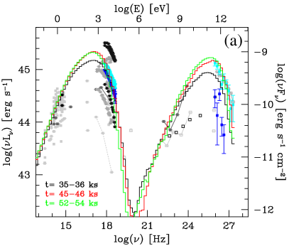
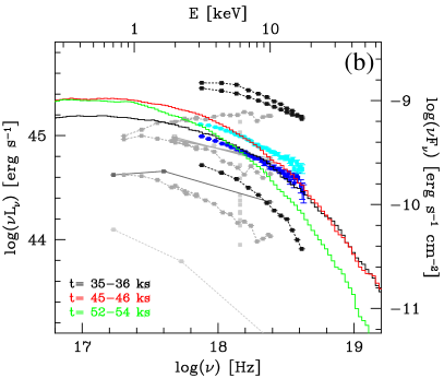
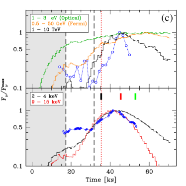
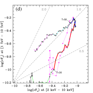
Figure 7: Summary of results for the case 3 (blob with pre-existing background electron population, with parameters adjusted to better match the TeV spectrum.) All panels, colors, symbols are the same used in Fig. 4.

4.5.1 Results

The resulting SEDs, light curves, and the X-ray vs. TeV flux-flux correlation are shown in Fig. 6a-d, the DCFs in Fig. 5c,d. This scenario does not reproduce the main features of the reference observations better than the first one.

1. The flare is asymmetric in TeV $\gamma$-rays and in the softer X-ray band. It remains symmetric for harder X-rays.

   The relative length of cooling and geometric time-scales is again an important factor, cleanly shown by the X-ray bands. In TeV $\gamma$-rays however this is compounded by the effect of LCTEs. The first steeper rise (up to $t\!=\!30$ ks) of TeV flux is driven by the increase of electrons as they are injected in the blob by the moving shock combined with the fact that we see a larger and larger fraction of the blob volume, modulated by external LCTE (see § 4.7). This is also signaled by the fact that the knee occurs at around the time when the observer would see the largest section of the blob (red dotted line in Fig. 6c). The slow rising, flat-top, phase ($30\!-\!45$ ks) of the TeV light curve is due to the increase of seed photons available at each location within the blob due to diffusion from the rest of the blob, delayed by internal LCTE. It’s a slow rise also because the high energy electrons responsible for most of the IC scattering to the TeV band are already cooling rapidly. At some point the radiation energy density in each location in the blob will stop increasing because enough time has passed for photons to diffuse throughout the blob. After that time the evolution is simply determined by particle cooling and external LCTE. Because the electrons emitting the bulk of the observed TeV flux have a cooling time larger than $R/c$, in this case the TeV flare decay shape is determined by cooling rather than LCTE.

2. As in case 1, the flux-flux amplitude correlation is reproduced only partially. The trend is almost quadratic during the rising phase of the flare, and it turns to sub-linear on the decaying phase, after a short horizontal shift corresponding to the flat top of the TeV light curve.

3. The path of the flux–flux diagram signals the presence of a time lag between the soft X-ray and the TeV $\gamma$-ray emission, which is shown in the DCF (Fig. 5d). The TeV $\gamma$-ray lags the 2-4 keV soft X-ray by about 2 kilo-seconds, comparable to the observation of the March 19 flare as in the first scenario. Also similar to case 1 is the soft lag between the two X-ray bands, opposite to what observed on 2001 March 19.

4. For what concerns the optical band, since we designed also this second scenario to address directly its minimal variability, it is not surprising that the light curve exhibits only a modest variation.

5. Finally, also in this scenario we have not been able to produce TeV $\gamma$-ray spectra as hard as the observations and in the end we limited ourselves to matching the flux level at around 1 TeV.

Some of the differences with respect to the first case are ultimately due to the weaker magnetic field making synchrotron cooling time-scales $\sim 60$% longer: for the highest energy electrons emitting in X-ray and TeV $\tau^{\prime}_{\mathrm{cool}}$ becomes longer than $R/c$. It is worth emphasizing that the decrease of $B$ is dictated by observational constraints, namely the relative luminosity of the synchrotron and IC components and the need to compensate for the absence of the additional source of seed photons for IC scattering provided in case 1 by the co-located ‘background’ component. This is in fact a good example of how the model is globally constrained.

4.6 Case 3: with pre-existing electron population, adjusted to better match the TeV spectrum

As we pointed out, in the previous two cases, the simulated SED in the TeV $\gamma$-ray range is softer than the observed spectra. To try to improve the match of the TeV part of the SED, we considered a modified version of the first scenario. We increased the Lorentz factor ($\Gamma\simeq 46$) and decreased the magnetic field strength ($B=0.035$ G), the goal being to move the inverse Compton peak to higher energy while leaving the synchrotron peak approximately unchanged. The parameters are: $R=1.5\times 10^{16}$ cm, $Z=2\times 10^{16}$ cm, $B=0.035$ G, $\Gamma=46$. At $t=0$ the ‘background’ electrons have the same broken power law distribution as in the first case, but with lower number density, $n_{\mathrm{e}}=1.56$ cm^-3. The volume is slightly larger yielding a total energy content of $2.9\times 10^{46}$ ergs.

The injected electrons have a power law distribution with $p=1.5$, $\gamma_{\mathrm{min}}=50$, $\gamma_{\mathrm{max}}=1.9\times 10^{5}$, $L^{\prime}_{\mathrm{inj}}=3.2\times 10^{40}$ erg/s. Injections starts in this case at $t^{\prime}_{\mathrm{start,inj}}=8\times 10^{5}$ s.

Results are integrated over $0.99971<\cos(\theta)<0.99981$, which corresponds to a Doppler factor range $37<\delta<57$.

4.6.1 Results

SEDs, light curves, and X-ray vs. TeV flux-flux correlation are shown in Fig. 7, and DCFs in Fig. 5e,f. The itemized summary of the main reference observations does not show improvements beyond the slightly higher VHE SED peak.

1. Because of the larger Doppler factor the electron emitting at the SED peaks have lower energy, which combined with a weaker magnetic field results in longer cooling time-scales (see eq. 12), in turn exceeding the source crossing time. This has the effect of increasing the asymmetry of the light curves in bands whose emission involves lower energy electrons and/or photons. The soft X-ray and TeV $\gamma$-ray light curves indeed have a slowly decaying tail.

2. Once again during the rising phase of the flare the $\gamma$-ray-X-ray correlation is approximately quadratic, until the peak of the X-ray light curve. After the TeV flare peak the correlation is approximately linear, as expected when the variation in both bands is driven only by the cooling of the (same) electrons, because the IC seed photons are emitted by particles with longer cooling time-scale.

3. The results concerning time-lags are equivalent to those of the other scenarios, perhaps with a hint of a smaller lag between TeV and softer X-ray. More extensive analysis would be necessary to quantify this possibility.

4. The slight shift of the IC peak to higher energy enables a better match with the observed spectra, although the actual spectral indices of the simulated SEDs remain softer than the observed values.

Further increases of the Doppler factor can still produce good SEDs, as long as we concurrently reduce the size of the volume. However, the light crossing time would rapidly become smaller than the observed flare duration, and it would have minimal impact on the observed phenomenology. Therefore the observed flare shapes must represent the true acceleration and cooling of the electrons, and the symmetry of the light curves must be caused by similar heating (or injection) and cooling time-scales.

4.7 Geometric Effects on Light Curves

There are complex geometry-related effects that have an impact not only on the shape of the observed light curve (e.g. its symmetry), but can also leave an imprint on other observables such as time lags and energy-dependent flare shape. Depending on how the particle injection and acceleration processes are distributed spatially, differences in physical time-scales for particles of different energy effectively may add a further geometric effect by inducing inhomogeneities (e.g. stratification) in the source (see also Chiaberge & Ghisellini, 1999; Sokolov et al., 2004).

We would like to illustrate with an extremely simple toy-model some aspects of the role of the geometry of the emitting region, and its interplay with some of the intrinsic physical time-scales, responsible for the fact that the peaks of the simulated X-ray light curves did not correspond to either the time when the shock exits the active region and injection is not present anywhere anymore, or to the time corresponding to the largest cross-section of the cylindrical volume along planes of equal observed times. In Figures 4c, 6c, 7c, these two times are marked as the second dashed grey line and the red-dotted line, respectively. Moreover, the shift changes with the light curve energy band as noticeable in the case of X-ray light curves.

To illustrate how time shifts are caused by the different size of the observable regions filled with electrons contributing most of the emission at those frequencies, we consider a purely geometrical model solely based on the ‘appearance’ of slices of different thickness through a cylinder.

Like in our real blob model, a shock is traveling along the axis of symmetry of the cylinder turning ‘on’ a thin local slice. Each point of this slice stays ‘on’ for a limited time, $\tau_{\mathrm{on}}$. We do not consider a variation of brightness with time, just an on/off state. We build light curves where ‘flux’ is simply the size of the volume that is seen ‘on’ by the observer at any given time. The ‘on’ volume visible at each time from the observer point of view is computed taking into account light travel times and it cuts through the cylinder along planes yielding constant arrival time to the observer. For an observer viewing the cylinder at an angle $\varphi$ with respect to its axis, the loci of points whose photons he sees simultaneously are planes with an inclination $\varphi/2$ with respect to the face of the cylinder ($90\degr-\varphi/2$ with respect to the cylinder axis). Figure 8 shows a 2D schematic of the geometry of the problem.

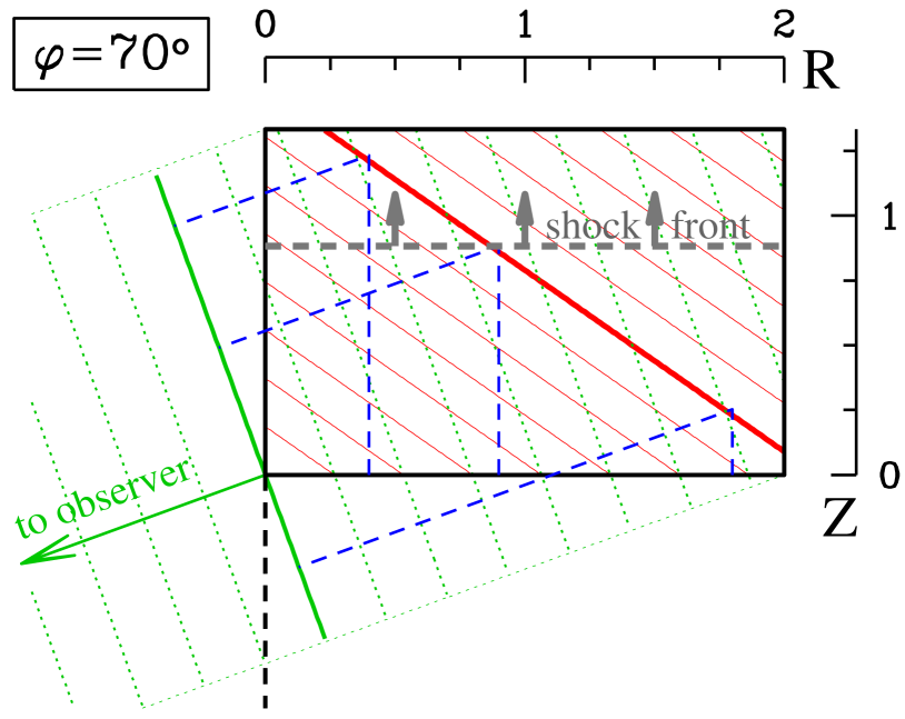
Figure 8: Diagram illustrating the geometry of the toy-model (see text, § 4.7). The black rectangle represents a side 2D view of the cylinder, with $R=1$ and $Z=4/3$ (same aspect ratio of our simulations). The grey dashed line represents the ‘shock front’ traveling at the speed of light through the cylinder, along its axis of symmetry, in the direction marked by the arrows. The green arrow represents the direction to the observer, while the green lines (solid and dotted) are planes perpendicular to the line of sight. In this example the viewing angle is $\varphi=70\degr$. The red lines represent the loci of points whose photons reach the observer simultaneously, taking into account the ‘shock‘ travel distance/time until of their activation and the light travel time to the observer since that moment. The blue dashed lines illustrate this by showing three paths of equal length from the beginning of the ‘flare’. The red loci form an angle $90\degr-\varphi/2$ with the line of sight or, equivalently, an angle $\varphi/2$ with the front face of the volume.

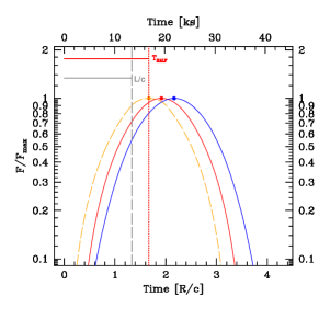
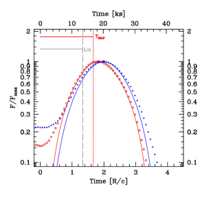
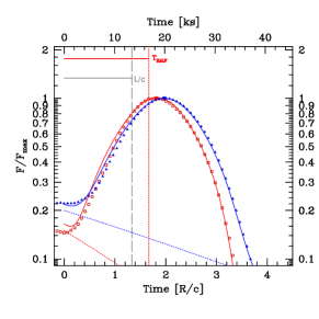
Figure 9: Light curves for a purely geometrical toy-model of the observations of a cylinder seen at an angle $\varphi=90\degr$ with respect to its axis. The meaning of the vertical lines is the same as in Fig. 4c, 6c, 7c, except that since the ‘injection’ begins at $t=0$, there is no first grey dashed line. (a) Three cases illustrating the time shift caused by the simple variation of $\tau_{\mathrm{on}}$. The (light) curves are computed for $\tau_{\mathrm{on}}=10^{-3}$ (orange), 0.5 (red), 1.0 (blue), in units of $R/c$. The orange case, with a $\tau_{\mathrm{on}}$ value yielding a negligible slice thickness, peaks at the expected time. (b) Attempt at matching light curves and simulation data without any baseline component contribution. The red curve is computed for $\tau_{\mathrm{on}}=0.35$, the blue for $\tau_{\mathrm{on}}=0.65$. The symbols are the simulated light curves of case 1, shown in Fig. 4c: red empty squares for 9$-$15 keV and blue triangles for 2$-$4 keV. (c) Same flare light curves combined with a slowly decaying baseline, with time-scale proportional to $\tau_{\mathrm{on}}$.

If the cylinder was moving with Lorentz factor $\Gamma$, because of relativistic aberration at a viewing angle $\theta\simeq 1/\Gamma$ we would be observing the radiation that in the comoving frame leaves the cylinder ‘sideways’, at 90$\degr$ from its axis. The observed frequencies would be blue-shifted and times compressed, but that would be simply a scaling factor applied uniformly to them and for convenience we can chose to use observed frequencies and times. Therefore observing the toy-model at $\varphi=90\degr$ is equivalent to observing the relativistically moving blob at $\theta=1/\Gamma$, and in turn this purely geometrical analysis captures some of the features of the realistic model studied in this paper.

The results are illustrated in Figure 9. In the first panel, we show the general features of the light curves obtained with this model, most importantly the effect of the change in the duration $\tau_{\mathrm{on}}$. In Figure 9a we plot the curves for three cases, showing the shift of the flare peak to later time as $\tau_{\mathrm{on}}$ increases. For very short $\tau_{\mathrm{on}}$ the maximum is reached at the expected time, that is when size of the plane that is the locus of points simultaneously seen by the observer (red lines in Fig. 8) is the largest possible for the given viewing angle. In general, however, the light curve peak will be shifted by $\Delta t=\tau_{\mathrm{on}}/2$. There is also a widening of the light curve, though much less noticeable than the peak shift. It is worth noting that at this extreme level of simplification geometric effects can not produce any asymmetry in the light curves.

We tried to reproduce with this toy-model the X-ray light curves from the simulations of the first scenario presented here. The results are shown in Figure 9b,c. The central panel shows the curves obtained by adjusting $\tau_{\mathrm{on}}$ to match the peak time of the two X-ray light curves (plotted with symbols), yielding a very satisfactory result for values around 0.35 and 0.65 $R/c$. However the overall shape of the flares can not be matched well without adding a baseline component, to mimic in some way the fact that in the simulations the blob was already ‘on’ at a low level prior to the beginning of the injection. We therefore added to the toy-model light curves a slowly decaying component, with an initial level such that the combination of the two components would match the data. Since in the simulations the pre-existing component is left to evolve (cool) starting at the beginning of the active phase, here we let the baseline component decay too. The visual matching is not critically sensitive to the exact values of the decay slopes, and to make the model more constrained we forced them to be in a fixed ratio with respect to the chosen $\tau_{\mathrm{on}}$, by considering that the cooling times of the electrons emitting the baseline photons are also related to their energies. For the results shown in Figure 9c the slope is equal to five times $\tau_{\mathrm{on}}$ for both cases.

The synchrotron cooling time-scale for electrons emitting in the $2-4$ keV and $9-15$ keV bands, following the approximate expression of eq. 12 are $\tau_{\mathrm{soft}}\simeq 0.73-1.04\,R/c$, $\tau_{\mathrm{hard}}\simeq 0.38-0.5\,R/c$. Given the steepness of the X-ray spectrum the emission in each band is dominated by the lower energy electrons, hence the longer $\tau$ is probably a more appropriate estimate. On the other hand, the above cooling time-scales only consider synchrotron cooling. Including some additional loss due to IC would decrease the value of $\tau$. In any case, the similarity between these crude estimates of cooling time-scales and the values of $\tau_{\mathrm{on}}$ corroborates the success of the geometrical toy-model at fitting the simulation light curves.

The ability of the purely geometrical toy-model to reproduce the two X-ray light curves is indeed remarkable. For X-rays this is facilitated by the fact that the synchrotron emission is independent on the internal delays due to photon diffusion that affect the evolution of the IC emission from the blob. It is not possible to apply a similar toy-model to the $\gamma$-ray light curves.

It is worth noting that although this test shows how dominant the effect of the geometry can be in shaping the light curve, at the same time we need to highlight that some geometry parameters, such as the ‘thickness’ of the visible slices, are in effect determined by the physical conditions of the emission region.

In this respect it is interesting to note that, at least in the setup of the scenarios presented in this work, despite the apparent dominance of the source geometry the effect of the energy dependent physics-induced geometrical factors is detectable. Hence multiwavelength datasets and time-resolved spectroscopy have the potential to disentangle them from the source geometry.

5 Discussion

We introduced a coupled Fokker–Planck and Monte Carlo code allowing us to study blazar phenomenology in unprecedented detail with a time dependent and multi-zone model properly taking into account all light travel time effects.

We presented three test scenarios, aimed at modeling the variability exhibited by Mrk 421 during the 2001 March 19 flare, and based on a relatively standard choice of parameters. The results of these tests are summarized in Table 2, side by side with the features observed in the actual multiwavelength observations (Fossati et al., 2008). There are a few fundamental issues that we wanted to address, which are common throughout the phenomenology of all well studied blue blazars.

1. The shape of the flares, often quasi-symmetric for a wide range of observational bands where the intensity variations are large (the main ones being X-ray and $\gamma$-ray).

2. The characteristics of the correlation between X-ray and $\gamma$-ray fluxes. There has been great interest in the slope of their relationship, in particular because of the observation of a quadratic, or higher order, relationship holding throughout some well sampled outbursts, challenging our understanding of the physical conditions and causes of the variability.

3. The phase of the correlation between variations in different bands, namely the existence of time lags and their duration.

None of the three test scenarios was able to reproduce all the characteristics of the 2001 March 19 flare. Two features have been particularly challenging to match: the relationship between X-ray and TeV $\gamma$-ray fluxes on the decay phase of the flare, and the intra-band X-ray time lag. Moreover, the shape (symmetry) of the flare light curves could be reproduced only by one of the three scenarios, case 1.

These aspects of phenomenology are among those more affected by the spatial extent and geometry of the source, whose influence varies with observed energy band because of the relative importance of geometrical and physical time-scales. The impact of the geometrical factor, both due to the source intrinsic structure and to the stratification of properties due to the physical processes, emphasizes the necessity of a code like the one we introduce here for modeling the variable high energy emission from blazar jets.

The difficulty of producing a quadratic relationship between the fluxes in the X-ray and $\gamma$-ray during the declining phase of the flare may indicate that radiative cooling cannot fully explain the electron cooling mechanism. The delayed evolution of the seed photon field due to internal LCTE compounds the problem. One alternative possibility could be a process causing energy loss over a wide range of electrons energies (such that the IC seed photons are also affected) on very similar/same time-scale, such as adiabatic cooling, which could be associated with expansion of the blob, or particle escape. They are often invoked in qualitative discussions and in the context of simpler models, treated by means of some phenomenological prescription. The addition of such mechanisms to the code in a proper astrophysical way is not immediate, but we are working on its implementation. The escape term present in the Fokker-Planck equation is actually neglected for these set of simulations. In a follow up work including particle acceleration and escape, this latter seems to be effective and we obtain a quadratic flux relationship and hard lags (e.g. Chen et al., 2011). About the effect of adiabatic expansion of the emitting blob, based on the simplified analysis of Katarzyński et al. (2005), Aharonian et al. (2009), argue against its viability once the implications of this expansion on the magnetic field and particle cooling are taken into account. Nevertheless, its effect should be assessed with actual time-dependent simulations of a source of finite size.

As to the hard intra-band X-ray lags, in Section 4.7 by means of a toy-model we illustrated an important factor affecting observations of time-lags: source ‘stratification’ combined with LCTE induces a systematic soft lag. The simulations presented in this work do not include an acceleration term, hence the lack of hard lags is not a complete surprise. Nevertheless, the induced systematic geometric soft lag introduces an additional constraint on viable electron acceleration and injection scenarios. In this respect, the results of the above mentioned study focused on X-ray lags (Chen et al., 2011) suggest that continuous acceleration, spatially extended (e.g. diffuse diffusive acceleration due to turbulence, Katarzyński et al., 2006), may be necessary, possibly accompanied by an achromatic energy loss mechanism. It is interesting that this type of scenario seems to be able to produce also a quadratic X-ray/TeV relationship throughout a flare.

One of the most interesting aspects of this analysis was the comparison between two possible hypotheses for the presence of an additional component contributing to the observed SED. The need for two components, a flaring and a quasi-steady one, to interpret some of the observations has become more evident with the improvement of multiwavelength observations (for an interesting decomposition of a Suzaku spectrum of Mrk 421 see Ushio et al., 2009). Disentangling these two components is necessary in order to understand the nature of the transient activity whose properties need to be seen more clearly. This decomposition might also yield information on the average properties of the relativistic jet, for which the less variable component might be more representative.

Table 2: Summary of Simulations Results

Feature	Obs.		Case 1		Case 2		Case 3
Flare symmetry
soft X-ray	Y		Y	$+$	N	$-$	N	$-$
hard X-ray	Y		Y	$+$	Y	$+$	Y	$+$
TeV $\gamma$-ray	Y		Y	$+$	N	$-$	N	$-$
Flux-Flux Correlation
trend up	2		2	$+$	2	$+$	2	$+$
trend down	2		1	$-$	1	$-$	1	$-$
Time Lags
X-ray $-$X-ray	hard (2 ks)		soft	$-$	soft	$-$	soft	$-$
X-ray $-$$\gamma$-ray	$\gamma$-ray (2 ks)		Y	$+$	Y	$+$	Y	$+$

We considered the two simplest possibilities: i) that the secondary component is due to a population of electrons that exists in the same region that will become active, and that will be affected by the flare and evolve with it. This pre-existing component can be interpreted as due to the remnants of a previous outburst. ii) That the secondary component is completely independent from the flare, and it contributes just a steady SED diluting the transient component from the observer point of view. Our simulations offer some hints as to their viability, and they favor the first type of scenario. One fundamental difference between the two alternatives concerns the production of IC emission, i.e. the TeV band. If the observed SED consists of the sum of two independent contributions, emitted by electrons at two different locations then the only seed photons for IC scattering will be those produced by the injected electrons themselves. Starting from an empty blob, the energy density of synchrotron seed photons needs some time to build up, which naturally results in a delay in the variation of the IC scattered $\gamma$-rays. This delay is caused by internal LCTE and it turned out to be quite significant as illustrated by the TeV light curve of case 2 (Fig. 6c), yielding a flat-top flare not seen in observations. That TeV light curve is in fact an excellent example of LCTEs at work and of the importance of a more advanced modeling code.

Naturally, the cases presented in this paper only represent an initial study aimed at investigating the importance of LCTE which for the first time could be fully accounted for. These results can not be considered conclusive. Nonetheless, despite their limited scope they make a strong case for a true time-dependent and multi-zone modeling.

The three scenarios discussed can be generally regarded as homogeneous blob scenarios. The magnetic field is the same throughout the simulation volume, and isotropic. For what concerns electrons, the initial setup is homogeneous and the injection is identical in all zones. It is, however, worth emphasizing that during the evolution of the simulation electrons properties become inhomogeneous because of the different radiative cooling they experience in different zones.

These simulations represent a first order implementation of a class of scenarios for blazar flares often discussed in the literature, envisaging a shock acting on a discrete blob/shell within the jet. We adopted a volume with relatively symmetric aspect ratio, to not depart too much from the sphere ‘implied’ by one-zone models while making it possible to appreciate the effects of geometry, and attributed the flare to the injection of a fresh electron population.

As discussed in Sections 4.1, 4.2, and 4.3 the main physical parameters are fairly well constrained and the results can be regarded as meaningful for what concerns the time-varying components of the model, as well as the nature of the secondary emission component. The simulations presented in this paper suggest that a simple injection in the radiating region of particles with a formed spectrum produced in a separate acceleration region whose emission is not significant, does not provide a satisfactory match with some basic observational facts. Moreover, the comparison of the background and foreground component scenarios, in particular with respect to the TeV $\gamma$-ray evolution, clearly favoring the first one (case 1), suggests that if a flare is caused by a change affecting the electron population it may be necessary for it to happen on a relatively hot blob, acting on the same particles, re-accelerating them. This in turn would support a scenario where flares are not fully independent of each other but rather occur in the same region.

5.1 Outlook

We are working on a few directions of expansion of this investigation. The main immediate focus is on the two unsolved issues of hard intra-band X-ray lags and X-ray-TeV flux correlation and we have introduced particle acceleration and escape (e.g. Chen et al., 2011).

Further areas of study concern inhomogeneities and different geometries, which can be easily studied with this code. We can introduce a spatial structure to the magnetic field, either static or changing according to some prescription, which could be motivated as caused by compression and amplification of the tangled field by a shock, and we plan to expand the code to deal with anisotropic magnetic field. We have started to simulate more ‘exotic’ geometries, e.g. elongated or flattened blobs, and the effect of an energy release in a small sub-region (bubble) embedded in the simulated volume.

A particularly timely line of investigation concerns red blazars like FSRQs. Because the peak of their high energy component occurs in the less accessible MeV–GeV band, they have received much more limited attention, except at the time of EGRET, that however lacked the sensitivity to follow even bright sources throughout their full variability cycles. Fermi/LAT has changed the status quo by providing continuous coverage of several bright blazars, and even more importantly by being able to detect them during their more quiescent phases. Among the most remarkable examples there are 3C 454.3 and PKS 1510$-$089 that already provided new clues about the nature of their $\gamma$-ray emission and the structure of the jet by the study of the correlated variations between $\gamma$-rays and their synchrotron or thermal emission (Abdo et al., 2009; Bonning et al., 2009; Marscher et al., 2010). Our code allows us to simulate EC scenarios, by illuminating the active region with an external radiation field with full treatment of the relativistic aberrations, thus allowing us to model external components with different spectral, spatial and temporal properties.

We would like to thank J. D. Finke for the invaluable help he provided during the development of this work. XC thanks Guy Hilburn for helpful discussions. We also acknowledge the anonymous referee for the pointed comments and suggestions that lead to a better manuscript. This research has been supported by NASA grants NAG5-11796 and NAG5–11853, Chandra AR9-0016X, and Fermi Guest Investigator award NNX10AO42G. GF thanks the European Southern Observatory for the extended hospitality in its Santiago offices. MB acknowledges support by NASA through Fermi Guest Investigator Grant NNX09AT82G and Astrophysics Theory Program Grant NNX10AC79G. This work was supported in part by the Shared University Grid at Rice funded by NSF under Grant EIA-0216467, and a partnership between Rice University, Sun Microsystems, and Sigma Solutions, Inc. This research has made use of NASA’s Astrophysics Data System and of the NASA/IPAC Extragalactic Database (NED) which is operated by the Jet Propulsion Laboratory, California Institute of Technology, under contract with the National Aeronautics and Space Administration.

References

- Abbott & Lucy (1985) Abbott, D. C., & Lucy, L. B. 1985, ApJ, 288, 679
- Abdo et al. (2009) Abdo, A. A. et al. 2009, ApJ, 699, 817
- Aharonian et al. (2009) Aharonian, F. et al. 2009, A&A, 502, 749
- Arbeiter et al. (2005) Arbeiter, C., Pohl, M., & Schlickeiser, R. 2005, ApJ, 627, 62
- Bednarek & Protheroe (1997) Bednarek, W., & Protheroe, R. J. 1997, MNRAS, 292, 646
- Bednarek & Protheroe (1999) —. 1999, MNRAS, 310, 577
- Blandford & Eichler (1987) Blandford, R., & Eichler, D. 1987, Phys. Rep., 154, 1
- Błażejowski et al. (2005) Błażejowski, M. et al. 2005, ApJ, 630, 130
- Błażejowski et al. (2000) Błażejowski, M., Sikora, M., Moderski, R., & Madejski, G. M. 2000, ApJ, 545, 107
- Bonning et al. (2009) Bonning, E. W. et al. 2009, ApJ, 697, L81
- Böttcher (2007) Böttcher, M. 2007, Ap&SS, 309, 95
- Böttcher & Chiang (2002) Böttcher, M., & Chiang, J. 2002, ApJ, 581, 127
- Böttcher et al. (2003) Böttcher, M., Jackson, D. R., & Liang, E. P. 2003, ApJ, 586, 389
- Böttcher & Liang (2001) Böttcher, M., & Liang, E. P. 2001, ApJ, 552, 248
- Böttcher et al. (2009) Böttcher, M., Reimer, A., & Marscher, A. P. 2009, ApJ, 703, 1168
- Canfield et al. (1987) Canfield, E., Howard, W. M., & Liang, E. P. 1987, ApJ, 323, 565
- Chang & Cooper (1970) Chang, J. S., & Cooper, G. 1970, Journal of Computational Physics, 6, 1
- Chen et al. (2011) Chen, X., Fossati, G., Liang, E., & Böttcher, M. 2011, Journal of Astrophysics and Astronomy, 10.1007/s12036-011-9045-0
- Chiaberge & Ghisellini (1999) Chiaberge, M., & Ghisellini, G. 1999, MNRAS, 306, 551
- Cohen et al. (2007) Cohen, M. H., Lister, M. L., Homan, D. C., Kadler, M., Kellermann, K. I., Kovalev, Y. Y., & Vermeulen, R. C. 2007, ApJ, 658, 232
- Coppi et al. (1993) Coppi, P., Blandford, R. D., & Rees, M. J. 1993, MNRAS, 262, 603
- Coppi (1992) Coppi, P. S. 1992, MNRAS, 258, 657
- Coppi & Blandford (1990) Coppi, P. S., & Blandford, R. D. 1990, MNRAS, 245, 453
- Costamante et al. (2001) Costamante, L. et al. 2001, A&A, 371, 512
- Crusius & Schlickeiser (1986) Crusius, A., & Schlickeiser, R. 1986, A&A, 164, L16
- Dermer (1998) Dermer, C. D. 1998, ApJ, 501, L157
- Dermer et al. (1992) Dermer, C. D., Schlickeiser, R., & Mastichiadis, A. 1992, A&A, 256, L27
- Donnarumma et al. (2009) Donnarumma, I. et al. 2009, ApJ, 691, L13
- Drury (1983) Drury, L. O. 1983, Reports on Progress in Physics, 46, 973
- Edelson & Krolik (1988) Edelson, R. A., & Krolik, J. H. 1988, ApJ, 333, 646
- Fabian et al. (2001a) Fabian, A. C., Celotti, A., Iwasawa, K., & Ghisellini, G. 2001a, MNRAS, 324, 628
- Fabian et al. (2001b) Fabian, A. C., Celotti, A., Iwasawa, K., McMahon, R. G., Carilli, C. L., Brandt, W. N., Ghisellini, G., & Hook, I. M. 2001b, MNRAS, 323, 373
- Fabian et al. (1986) Fabian, A. C., Guilbert, P. W., Blandford, R. D., Phinney, E. S., & Cuellar, L. 1986, MNRAS, 221, 931
- Finke (2007) Finke, J. D. 2007, PhD thesis, Ohio University
- Fossati et al. (2008) Fossati, G. et al. 2008, ApJ, 677, 906
- Fossati et al. (2000a) —. 2000a, ApJ, 541, 153
- Fossati et al. (2000b) —. 2000b, ApJ, 541, 166
- Fossati et al. (1998) Fossati, G., Celotti, A., Ghisellini, G., Maraschi, L., & Comastri, A. 1998, MNRAS, 299, 433
- Gaisser (1991) Gaisser, T. K. 1991, Cosmic Rays and Particle Physics (Cambridge: Cambridge University Press)
- Ghisellini et al. (1998) Ghisellini, G., Celotti, A., Fossati, G., Maraschi, L., & Comastri, A. 1998, MNRAS, 301, 451
- Ghisellini et al. (1988) Ghisellini, G., Guilbert, P. W., & Svensson, R. 1988, ApJ, 334, L5
- Ghisellini & Madau (1996) Ghisellini, G., & Madau, P. 1996, MNRAS, 280, 67
- Ghisellini et al. (2010) Ghisellini, G., Tavecchio, F., Foschini, L., Ghirlanda, G., Maraschi, L., & Celotti, A. 2010, MNRAS, 402, 497
- Giebels et al. (2007) Giebels, B., Dubus, G., & Khélifi, B. 2007, A&A, 462, 29
- Graff et al. (2008) Graff, P. B., Georganopoulos, M., Perlman, E. S., & Kazanas, D. 2008, ApJ, 689, 68
- Kataoka (2000) Kataoka, J. 2000, PhD thesis, Univ. of Tokyo
- Kataoka et al. (2000) Kataoka, J., Takahashi, T., Makino, F., Inoue, S., Madejski, G. M., Tashiro, M., Urry, C. M., & Kubo, H. 2000, ApJ, 528, 243
- Katarzyński et al. (2006) Katarzyński, K., Ghisellini, G., Mastichiadis, A., Tavecchio, F., & Maraschi, L. 2006, A&A, 453, 47
- Katarzyński et al. (2005) Katarzyński, K., Ghisellini, G., Tavecchio, F., Maraschi, L., Fossati, G., & Mastichiadis, A. 2005, A&A, 433, 479
- Katarzyński et al. (2008) Katarzyński, K., Lenain, J., Zech, A., Boisson, C., & Sol, H. 2008, MNRAS, 390, 371
- Kellermann & Pauliny-Toth (1981) Kellermann, K. I., & Pauliny-Toth, I. I. K. 1981, ARA&A, 19, 373
- Kirk et al. (1998) Kirk, J. G., Rieger, F. M., & Mastichiadis, A. 1998, A&A, 333, 452
- Krawczynski et al. (2002) Krawczynski, H., Coppi, P. S., & Aharonian, F. 2002, MNRAS, 336, 721
- Krawczynski et al. (2004) Krawczynski, H. et al. 2004, ApJ, 601, 151
- Krawczynski et al. (2001) —. 2001, ApJ, 559, 187
- Levinson (2006) Levinson, A. 2006, International Journal of Modern Physics A, 21, 6015
- Li & Kusunose (2000) Li, H., & Kusunose, M. 2000, ApJ, 536, 729
- Makino (1999) Makino, F. 1999, in Astronomical Society of the Pacific Conference Series, Vol. 159, BL Lac Phenomenon, ed. L. O. Takalo & A. Sillanpää, 190
- Mannheim (1998) Mannheim, K. 1998, Science, 279, 684
- Maraschi et al. (1999) Maraschi, L. et al. 1999, ApJ, 526, L81
- Maraschi et al. (1992) Maraschi, L., Ghisellini, G., & Celotti, A. 1992, ApJ, 397, L5
- Marscher et al. (2010) Marscher, A. P. et al. 2010, ApJ, 710, L126
- Marscher & Travis (1996) Marscher, A. P., & Travis, J. P. 1996, A&AS, 120, 537
- Mastichiadis & Kirk (1997) Mastichiadis, A., & Kirk, J. G. 1997, A&A, 320, 19
- McHardy et al. (2007) McHardy, I., Lawson, A., Newsam, A., Marscher, A. P., Sokolov, A. S., Urry, C. M., & Wehrle, A. E. 2007, MNRAS, 375, 1521
- Nayakshin & Melia (1998) Nayakshin, S., & Melia, F. 1998, ApJS, 114, 269
- Press et al. (1992) Press, W., Teukolsky, S., Vetterling, W., & Flannery, B. 1992, Numerical Recipes, the art of scientific computing second edition (Cambridge University Press)
- Protheroe (1996) Protheroe, R. J. 1996, in Towards the Millennium in Astrophysics: Problems and Prospects, Erice 1996, eds. M.M. Shapiro and J.P. Wefel (World Scientific: Singapore)
- Protheroe (2002) Protheroe, R. J. 2002, PASA, 19, 486
- Punch et al. (1992) Punch, M. et al. 1992, Nature, 358, 477
- Rachen (2000) Rachen, J. P. 2000, in Proc. of GeV-TeV Gamma Ray Astrophysics Workshop: Towards a Major Atmospheric Cherenkov Detector VI, Snowbird, eds. B.L. Dingus, M.H. Salamon, D.B. Kieda, AIP Conf. Proc. 515 (New York: AIP)., 41
- Ravasio et al. (2002) Ravasio, M. et al. 2002, A&A, 383, 763
- Rebillot et al. (2006) Rebillot, P. F. et al. 2006, ApJ, 641, 740
- Rieger & Duffy (2004) Rieger, F. M., & Duffy, P. 2004, ApJ, 617, 155
- Rieger & Duffy (2006) —. 2006, ApJ, 652, 1044
- Rybicki & Lightman (1979) Rybicki, G. B., & Lightman, A. P. 1979, Radiative Processes in Astrophysics, John Wiley & Sons ((New York): John Wiley & Sons)
- Sambruna et al. (2000) Sambruna, R. M. et al. 2000, ApJ, 538, 127
- Sikora et al. (1994) Sikora, M., Begelman, M. C., & Rees, M. J. 1994, ApJ, 421, 153
- Sikora et al. (2001) Sikora, M., Błażejowski, M., Begelman, M. C., & Moderski, R. 2001, ApJ, 554, 1
- Sikora & Madejski (2001) Sikora, M., & Madejski, G. 2001, in American Institute of Physics Conference Series, Vol. 558, , 275–288, booktitle was: American Institute of Physics Conference Series
- Sikora et al. (2009) Sikora, M., Stawarz, Ł., Moderski, R., Nalewajko, K., & Madejski, G. M. 2009, ApJ, 704, 38
- Sokolov & Marscher (2005) Sokolov, A., & Marscher, A. P. 2005, ApJ, 629, 52
- Sokolov et al. (2004) Sokolov, A., Marscher, A. P., & McHardy, I. M. 2004, ApJ, 613, 725
- Stawarz & Ostrowski (2002) Stawarz, Ł., & Ostrowski, M. 2002, ApJ, 578, 763
- Stern et al. (1995) Stern, B. E., Begelman, M. C., Sikora, M., & Svensson, R. 1995, MNRAS, 272, 291
- Takahashi et al. (2000) Takahashi, T. et al. 2000, ApJ, 542, L105
- Takahashi et al. (1996) —. 1996, ApJ, 470, L89
- Tanihata et al. (2004) Tanihata, C., Kataoka, J., Takahashi, T., & Madejski, G. M. 2004, ApJ, 601, 759
- Tavecchio et al. (1998) Tavecchio, F., Maraschi, L., & Ghisellini, G. 1998, ApJ, 509, 608
- Tavecchio et al. (2001) Tavecchio, F. et al. 2001, ApJ, 554, 725
- Tramacere et al. (2007) Tramacere, A., Massaro, F., & Cavaliere, A. 2007, A&A, 466, 521
- Ulrich et al. (1997) Ulrich, M.-H., Maraschi, L., & Urry, C. M. 1997, ARA&A, 35, 445
- Urry & Padovani (1995) Urry, C. M., & Padovani, P. 1995, PASP, 107, 803
- Ushio et al. (2009) Ushio, M. et al. 2009, ApJ, 699, 1964
- Virtanen & Vainio (2005) Virtanen, J. J. P., & Vainio, R. 2005, A&A, 439, 461