Star Formation Activity in the Galactic H ii Complex S255-S257

Abstract

We present results on the star-formation activity of an optically obscured region containing an embedded cluster (S255-IR) and molecular gas between two evolved H ii regions S255 and S257. We have studied the complex using optical, near-infrared (NIR) imaging, optical spectroscopy and radio continnum mapping at 15 GHz, along with Spitzer-IRAC results. It is found that the main exciting sources of the evolved H ii regions S255 and S257 and the compact H ii regions associated with S255-IR are of O9.5 - B3 V nature, consistent with previous observations. Our NIR observations reveal 109 likely young stellar object (YSO) candidates in an area of $\sim$ 4^′.9 $\times$ 4^′.9 centered on S255-IR, which include 69 new YSO candidates. To see the global star formation, we constructed the $V-I/V$ diagram for 51 optically identified IRAC YSOs in an area of $\sim$ 13^′ $\times$ 13^′ centered on S255-IR. We suggest that these YSOs have an approximate age between 0.1 - 4 Myr, indicating a non-coeval star formation. Using spectral energy distribution (SED) models, we constrained physical properties and evolutionary status of 31 and 16 YSO candidates outside and inside the gas ridge, respectively. The models suggest that the sources associated within the gas ridge are of younger population (mean age $\sim$ 1.2 Myr) than the sources outside the gas ridge (mean age $\sim$ 2.5 Myr). The positions of the young sources inside the gas ridge at the interface of the H ii regions S255 and S257, favor a site of induced star formation.

1 Introduction

OB stars have the most dramatic influence on the evolution of surrounding medium, thereby regulating the star-formation activity of a complex. However, their evolution in a clustered environment and how they interact with the cold interstellar medium and process local gas to form new generation young stars is still not clear. Ultracompact (UC) H ii regions are manifestations of newly formed massive (O or early B) stars deeply embedded in the parental cloud. The UC H ii regions further evolve into the less obscure stage of compact and classical H ii regions. During the expansion they may sweep low density material forming dense layers of gas or interact with pre-existing dense clumps leading to density enhancement. In both the cases, matter at a later stage becomes unstable against self gravity and may lead to new star formation (Elmegreen & Lada 1977). However, the expansion usually takes place in non-homogeneous medium and the surroundings of the H ii regions are generally rich in molecular chemistry, which result in a complicated morphology. Therefore, a detailed study of the star-forming region (SFR) at various wavebands is necessary to trace the evolutionary status of young sources and star-formation scenario of an H ii environment. In this paper, we present results of an optically obscured young massive SFR, located between two evolved H ii regions, namely S255 and S257 (Sharpless 1959).

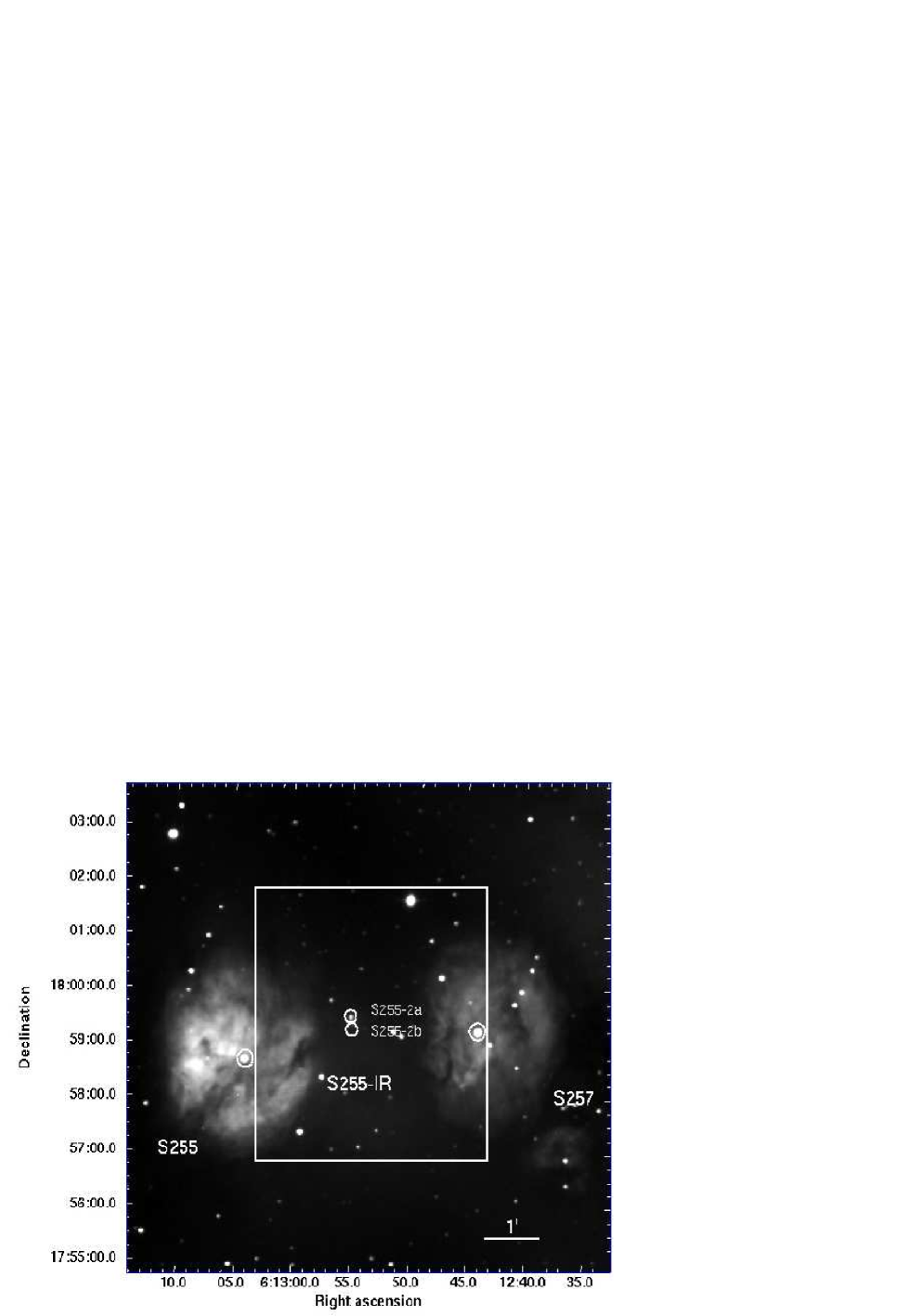
Figure 1: H$\alpha$+continuum image of the ionized gas associated with S255-S257 region obtained with ST (see Table 1) using the same set up described in Samal et al. (2007). The FOV is $\sim$ 10^′.0 $\times$ 9^′.5. The square box represents the observed region of the embedded cluster in NIR bands. The individual H ii regions and the cluster S255-IR are also marked. The circles represent the ionizing sources of the H ii regions, for which we have obtained optical spectroscopic information. North is up and east is to the left. RA and DEC coordinates are in J2000 epoch.

The photometric spectral type suggests the exciting sources of S255 and S257 are B0V (Moffat et al. 1979) and B0.5V (Reid 2008) type of stars. These two H ii regions are itself a part of a larger complex consisting of five H ii regions namely S254, S255, S256, S257 and S258. The complex is situated at a distance of $\sim$ 2.5 kpc (Russeil, Adami, & Georgelin 2007) and is a part of Gemini OB association (Huang & Thaddeus 1986). In the present study, we have adopted the distance of 2.5 kpc for our analysis. However, we also derived distance to the region using spectroscopic observations that come out to be close to the value of 2.5 kpc (see Section 3). A cluster S255-IR (also called as S255-2) containing infrared (IR)-excess sources (Howard, Pipher, & Forrest 1997) is embedded in the optically obscured region and is also associated with compact and UC Hii  regions, namely S255-2a, S255-2b, and S255-2c, whose exciting sources are B1 zero-age-main-sequence (ZAMS) stars (Snell & Bally 1986), of which two are optically visible. Radio observations also reveal an UC Hii  region $\sim$ 1^′ north of S255-2, which is a far-IR source detected by Jaffe et al. (1984) and is called S255N. Its total luminosity is approximately twice that of S255-IR (5 $\times$ 10⁴$L_{\odot}$ ; Minier et al. 2005). Sub-millimeter and millimeter emissions show large column of gas and dust with sub-structures (Zinchenko, Henning, & Schreyer 1997; Klein et al. 2005; Minier et al. 2005; Zinchenko, Caselli, & Pirogov 2009), elongated along the north-south directions and sandwiched between the two H ii regions S255 and S257. Figure 1 shows the H$\alpha$ continuum image, where individual H ii regions are marked. The dark lane between S255 and S257 is the subject of the present study and is devoid of optical stellar sources. However, this region shows several signatures of recent star formation such as: IR-excess sources (Howard, Pipher, & Forrest 1997; Miralles et al. 1997), Herbig-Haro objects (Miralles et al. 1997), compact and UC Hii  regions (Snell & Bally 1986; Kurtz, Churchwell, & Wood 1994), dense millimeter cores (Cyganowski, Brogan, & Hunter 2007) and masers (Goddi et al. 2007), therefore indicating that star formation is currently active in the dark lane. Since the dark lane contains a lot of gas and dust, as found by previous authors, hereafter we refer to this as “gas ridge” for further discussion in the paper.

A number of efforts were made in an attempt to combine various observed components into a coherent model to understand star-formation activity in the complex (Heyer et al. 1989; Carpenter 1995a,b; Chavarría et al. 2008). Here, we extend this work with our new observations, as part of our ongoing mutiwavelength investigation of star formation in and around Galactic H ii regions (e.g. Ojha et al. 2004a, 2004b, 2004c; Tej et al. 2006; Samal et al. 2007; Pandey et al. 2008; Samal et al. 2010). We studied the nature of stellar population in the gas ridge between S255-S257 with high resolution NIR observations covering an area of $\sim$ 4^′.9 $\times$ 4^′.9 of the gas ridge, along with radio continuum imaging at 14.94 GHz. Using spectroscopic observations we attempted to establish that the ionizing sources of the S255, S257 and the compact H ii regions of S255-IR cluster share a common plane in the sky. In order to unravel the star formation history, we also identified and characterized the stellar population beyond the gas ridge, using optical photometry in conjunction with mid-infrared (MIR) photometry from Chavarría et al. (2008), for an area of $\sim$ 13^′ $\times$ 13^′. We used Robitaille’s SED models for subsets of stellar sources in the gas ridge as well as outside to assess their likely evolutionary status. Our findings suggest that the sources in the gas ridge show signature of younger population. Since the gas ridge is sandwiched between two optically visible H ii regions, we tried to interpret a possible star formation scenario in the gas ridge. We have organised this paper as follows: In Section 2, we describe our observations and the reduction procedures. Section 3 describes spectral type of the ionizing sources of optically visible H ii regions and their possible associations. Section 4 describes the general morphology and nature of stellar sources and embedded cluster S255-IR. In Section 5, we discuss the age and mass of the stellar sources beyond the gas ridge. Section 6 describes the SED modeling of stellar sources. Section 7 is devoted to discussion on star formation scenario in the complex. We present the main conclusions of our results in Section 8.

2 Observations

2.1 Near-Infrared

The imaging observations of the S255 SFR centered on $\alpha_{2000}=06^{h}12^{m}53^{s}$, $\delta_{2000}=+17^{\circ}59^{\prime}21^{\prime\prime}$ in the $J$ ($\lambda$ = 1.25 $\mu$m), $H$ ($\lambda$ = 1.63 $\mu$m), and $K_{\rm s}$ ($\lambda$ = 2.14 $\mu$m) bands were obtained on 2000 October 13 with the 2.2 m UH telescope and SIRIUS, a three-color simultaneous camera (Nagashima et al. 1999; Nagayama et al. 2003). In this set up, each pixel of the 1024 $\times$ 1024 HgCdTe array corresponds to 0^′′.28 yielding a field of view (FOV) of $\sim$ 4^′.9 $\times$ 4^′.9 on the sky. A sky field which is 10^′ south of the target position (centered on $\alpha_{2000}=06^{h}12^{m}53^{s}$, $\delta_{2000}=+18^{\circ}09^{\prime}26^{\prime\prime}$) was also observed and used for sky subtraction. We obtained 18 dithered frames each of 20s, thus giving a total integration time of 360s in each band. The observing conditions were photometric and the average FWHM during the observing period was $\sim$0^′′.7-0^′′.9. Photometry was done using the PSF algorithm of DAOPHOT package (Stetson 1987) in IRAF, following the same procedure described in Samal et al. (2010). The photometric calibration was done by observing the standard star P9107 in the faint NIR standard star catalog of Persson et al. (1998) at air masses closest to the target observations. A comparison of present photometry with that of 2MASS photometry as a function of $J$ mag for the common sources is shown in Figure 2, where the 2MASS sources with photometric error $\leq$ 0.1 mag and ‘read-flag’ values between 1 to 3 are selected to ensure good quality (see Samal et al. 2010 for description). We find that the photometric scatter in magnitude increases at the fainter end, whereas the mean photometric uncertainties are $\leq$ 0.1 mag in all the three bands. Absolute position calibration of the detected sources was achieved using the coordinates of 20 isolated bright 2MASS sources. The astrometric accuracy is estimated to be $\sim$ 0^′′.05. To plot the data in color-color (CC) and color-magnitude (CM) diagrams, the $JHK_{\rm s}$ data were transformed to California Institute of Technology (CIT) system using the relations given by Nagashima et al. (2003).

2.2 Optical

2.2.1 Photometric Observations

The CCD $BV{(I)}_{c}$ observations of the S255 region centered on $\alpha_{2000}=06^{h}12^{m}54^{s}$, $\delta_{2000}=+17^{\circ}59^{\prime}11^{\prime\prime}$, were acquired on 2004 December 15, using the CCD camera mounted on the 104-cm Sampurnanand telescope (ST) of ARIES, Nainital (Sagar et al. 1999). In this set up, each pixel of the CCD corresponds to 0^′′.37 and yielding a field of view of $\sim$ 13^′ $\times$ 13^′ on the sky. The FWHM of the star images was $\sim$ 2^′′.5. To determine the atmospheric extinctions and to calibrate the CCD systems, we observed standard stars in the SA98 field (Landolt 1992) and short exposures of the target field using the ST on 2009 October 14. The observing conditions were photometric and the average FWHM during the observing period was $\sim$ 1^′′.8. The CCD data frames were reduced using DAOPHOT-II software (Stetson 1987) following the same procedure described in Samal et al. (2010). The standard deviations in the standardization residual, $\Delta$, between standard and transformed $V$ magnitude and colors are found to be less than 0.02 mag. We generated secondary standards from the short exposure images on 2009 October 14 to standardize the data observed on 2004 December 15. The mean and standard deviation of the photometric difference between the common stars of the target sources at $B$, $V$ and $I_{c}$ bands on both the nights are 0.009 $\pm$ 0.037, 0.006 $\pm$ 0.031 and 0.016 $\pm$ 0.054 respectively, therefore, we expect a calibration error less than $\sim$ 0.05 mag in all the bands. When brighter stars were saturated on deep exposure frames, their magnitudes have been taken from short exposure frames to make the final catalog. Since the photometric errors become large ($\geq$ 0.1 mag) for stars fainter than $V\simeq 21.6$ mag, the measurements beyond this magnitude limit are not used in the present study. An astrometric solution for the detected stars in the frame was determined using 15 isolated moderately bright stars with their positions from the 2MASS catalog and a position accuracy of better than $\pm$0^′′.1 has been achieved.

2.2.2 Spectroscopic Observations

We obtained optical spectra of the ionizing sources of S255 and S257, using 2-m telescope at IUCAA Girawali Observatory (IGO) on 2008 January 11. We used IUCAA Faint Object Spectrograph (IFOSC) with a silt of 1^′′.5 width in combination with a grism (IFOSC7) in the wavelength range 3800-6840 Å  at a spectral dispersion of 1.4 Å  pixel^-1. The spectra of the ionizing sources of S255-2a and S255-2b were obtained using 2.01-m Himalayan Chandra Telescope (HCT) on 2009 December 20 and 2010 January 18, respectively. The instrument is equipped with a SITe 2K $\times$ 4K pixel CCD. We used Himalaya Faint Object Spectrograph Camera (HFOSC) with a silt of 1^′′.9 width in combination with a grism (Gr 7) in the wavelength range of 3500-7000 Å  at a spectral dispersion of 1.45 Å  pixel^-1. The observing conditions were photometric, with a typical seeing of 1^′′.2 to 1^′′.3 during the nights. The one-dimensional spectra were extracted and wavelength calibrated following the procedure described in Samal et al. (2010). An rms scatter of 1 Å  is expected in the wavelength calibration.

The log of observations is given in Table 1.

2.3 Radio Continuum Imaging

We have also analysed the data of S255-IR at 14.94 GHz, taken from the National Radio Astronomy Observatory (NRAO) data archive (Project ID: AM697), obtained using the Very Large Array (VLA) in the D configuration. The observation was carried out in 28 November 2001. The flux calibrator was 0542+498 and 0625+146 was used as a phase calibrator. The NRAO AIPS was used for the reduction of the data. The estimated uncertainty of the flux calibration was within 5%. The image of the field was formed by the Fourier inversion and cleaning algorithm task IMAGR, with a Briggs weighting function (robust factor = 0) halfway between uniform and natural weighting. We applied two iterations of phase self-calibration to improve the map. The resulting image has a beam size of $\sim$ 4^′′.4 $\times$ 4^′′.2 and the rms noise in the map is 0.11 mJy/beam.

3 Ionizing Sources and the Ionized Gas Distribution

The one-dimensional spectra of the ionizing sources of S257, S255, S255-2a, and S255-2b in the range 3950-4950 Å are shown in Figure 3. We classified the observed spectra by comparing with those given by Walborn & Fitzpatrick (1990). In the case of O-type stars, the classifications of different subclasses are based on the strengths of the He ii line at 4541 Å  and He i line at 4471 Å. The equal strength of the lines implies a spectral type of O7, whereas the lesser the strength of 4541 Å  line as compared to 4471 Å  line implies a spectral type later than O7. The O-type luminosity class V spectra also have a strong He ii 4686 Å  in absorption. The main characteristics of early B-type stars are the absence of He ii lines, which are still present in late O-type stars. If the spectrum displays He ii line at $\sim$ 4200 Å, and weak He ii line at 4686 Å, along with OII/CIII blend at $\approx$ 4650 Å, this indicates the spectral type of the star must be earlier than B1. Specifically, He ii line at 4200 Å  is seen in stars of spectral type B0.5-B0.7. The presence of the He i lines in absorption constrains the spectral types to earlier than B5-B7. The He i lines may however be affected by the intense nebular emissions, which may fill the stellar absorption features of Balmer lines. It is not easy to subtract such emissions, which may be misleading to the spectral classification. The absence of significant Si ii line at 4128 Å  and presence of very weak Mg ii 4481 Å  line in the spectra indicate a spectral type earlier than B2 and the contributions of these lines increase towards spectral types later than B2 (Walborn & Fitzpatrick 1990). By comparing the strength of various lines, we classified the most probable spectral types of the ionizing sources of S255, S257 and S255-2a as O9.5, B0.5 and B2 respectively. The poor signal-to-noise ratio of the spectrum of the ionizing source of S255-2b limits the accuracy of classification, but the spectrum shows the signature of an early-B type star, possibly B2-B3. The luminosity criterion depends mainly upon the ratios of Si iii 4553 Å to He i 4387 Å and Si iv 4089 Å to He i 4121 Å, which shows a smooth progression along the main-sequence (MS) points to supergiant class. Though the assessment of luminosity class is difficult from the present spectra, we favor the luminosity as class V for the ionizing sources of S255 and S257 due to the presence of He ii 4686 Å and Si iii 4553 Å lines in absorption. As both S255-2a and S255-2b have characteristics comparable to those of compact H ii regions (Snell & Bally 1986), they are therefore not dynamically evolved objects. According to Meynet et al. (1994), an 18 $M_{\odot}$ star (corresponds to B0 spectral type) has MS lifetime of $\sim$ 8 Myr. Therefore, the luminosity class V seems to be more plausible for the ionizing sources of S255-2a and S255-2b.

To obtain the distance of S255-2a, we estimated the visual extinction ($A_{V}$) as 5.30 mag of the ionizing source, using a standard value of R_V $=$ 3.12 and adopting an intrinsic color $(B-V)_{0}$ = -0.24 (Cox 2000) for a B2 MS star, along with our measured photometric color $(B-V)$ = 1.46. Using the M_V -spectral type calibration table from Russeil (2003), the distance turns out to be 2.6 kpc. For the ionizing sources of S255 and S257 regions, we adopted magnitudes and colors from Moffat et al. (1979) as the sources are saturated in our photometry. For S255, we find $E(B-V)$ = 1.18 mag using $(B-V)$ = 0.88 and $(B-V)_{0}$ = -0.30, which corresponds to $A_{V}$ = 3.68 mag. Similarly, for S257, we find $E(B-V)$ = 0.87 mag using $(B-V)$ = 0.57 and $(B-V)_{0}$ = -0.30, which corresponds to $A_{V}$ = 2.71 mag. Following the same procedure as discussed above, the distance turns out to be 2.7 and 2.3 kpc for S255 and S257, respectively. The above analysis suggests probable association among the sources. The resulting average distance (2.53 $\pm$ 0.21 kpc) for the complex agrees well with the average distance 2.46 $\pm$ 0.17 kpc obtained by Russeil, Adami, & Georgelin (2007). There is however some ambiguity concerning the distance to the region. A number of authors suggested that the whole region corresponds to a cloud complex at 2.3 - 2.6 kpc (Chavarría et al. 2008 and references therein), which is also supported by our distance estimation. Therefore, in the present work we have adopted a distance of 2.5 kpc for further analysis. However, it is worth mentioning a recent study by Rygl et al. (2010) of the S255-IR region, which reported a distance of $\sim$ 1.6 kpc.

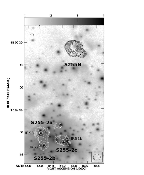
Figure 4: $K_{\rm s}$-band image in logarithmic scale overlaid with the VLA radio continuum contours at 14.94 GHz. The contour levels are at 0.11 $\times$ (3, 4, 5, 7, 10, 14, 19, 25, 32, 38, 50) mJy/beam, where $\sim$ 0.11 mJy/beam is the rms noise in the map at a resolution of $\sim$ $4\arcsec.4\times 4\arcsec.2$. The ionizing sources of the compact and UC Hii  regions S255-2a, S255-2b and S255-2c, are labeled with IRS3, IRS2 and IRS1b respectively, for further discussion in the paper (see Section 4.1)

The S255-IR region is a cluster forming environment which contains a number of OB-stars (Howard, Pipher, & Forrest, 1997), of which only two are visible in the optical band. Previous observations at 5 GHz show that this SFR usually contains four centimeter continuum sources (Snell & Bally 1986). Since the emissions from UC Hii and hyper-compact H ii regions are optically thick at this frequency, we analysed the radio continuum emission at 14.94 GHz obtained with VLA. Figure 4 shows contours of the 14.94 GHz radio free-free emission overlaid onto the $K_{\rm s}$-band image. The map mainly shows five compact radio emissions and four of them are marked in the figure as per nomenclature by Snell & Bally (1986). However, we detected one extra source that has not been previously identified in the literature. Though the 5 GHz map by Snell & Bally (1986) shows some weak radio emission approximately at the position of the source, the flux value of the source is not mentioned in their paper. Hence, to conclude whether the source is an extragalactic radio object or the true UC Hii region, one needs spectral index measurement which requires emission at two frequencies. Due to unavailability of the flux measurement at other frequencies, in the present analysis, we tentatively do not consider this radio source as a possible UC Hii region. However, the spectral indices between 5 GHz and the 14.94 GHz of the other radio sources suggest thermal origin. The regions of recent star formation in the $K_{\rm s}$-band image are traced by the bright nebulosity, whereas the H ii regions detected in centimeter surveys trace the high mass star-forming environment. It is well established that formation of high mass stars in young complexes is accompanied by a cluster of less massive sources. Hence, the NIR point sources in Figure 4 are likely candidates of intermediate to low mass stars. Out of the five compact radio emissions, the most intense emission associated with components S255N and S255-2c seems to be elongated along the east-west direction.

To derive the physical properties of the thermal radio sources, we measured peak position, integrated flux density and angular diameter deconvolved from the beam by fitting a two-dimensional elliptical Gaussian using the task JMFIT in AIPS. We calculated the physical parameters assuming the simplest geometry of uniform spherical model. The physical parameters are: $n_{e}$, the rms electron density; $EM$, the emission measure; $\tau$_c, the optical depth; $N_{Lyc}$, the number of Lyman continuum photons for a spherically symmetric H ii region and the ZAMS spectral type of the ionizing source. The ZAMS spectral type has been estimated from the $N_{Lyc}$ and the calibration table of Panagia (1973), for an electron temperature of 10⁴ K. These parameters were derived from the measured angular diameter and integrated flux density and using the formulae given by Panagia & Walmsley (1978) and Mezger & Henderson (1967) for spherical, homogeneous nebulae. The derived physical parameters are listed in Table 3. Since we derived the average properties, the rms electron density of the H ii regions is expected to be lower than the density at the peak positions. The spectral types suggest that all the sources are ionized by massive early B-type ZAMS stars and their physical parameters point to the evolutionary class between compact and UC Hii regions (Kurtz et al. 2000). Since the compact and UC Hii regions are not dynamically evolved objects, this indicates that the massive star formation has started recently at various locations of the gas ridge, whereas, the larger sizes and lower electron density values estimated from the 1.4 GHz observation by Snell & Bally (1986) for the H ii regions S255 (size $\sim$ 1.16 pc, n_e $\sim$ 100 cm^-3) and S257 (size $\sim$ 0.87 pc, n_e $\sim$ 111 cm^-3), indicate that both are in an advanced stage of evolution. This confirms that the ionizing sources of S255 and S257 are in a more evolved stage than the massive stars in the gas ridge.

4 Embedded Cluster

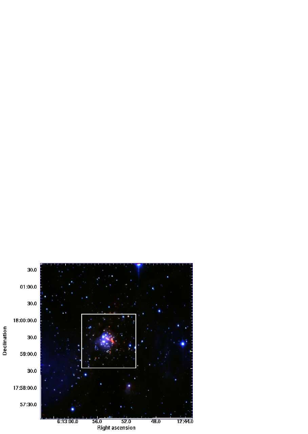
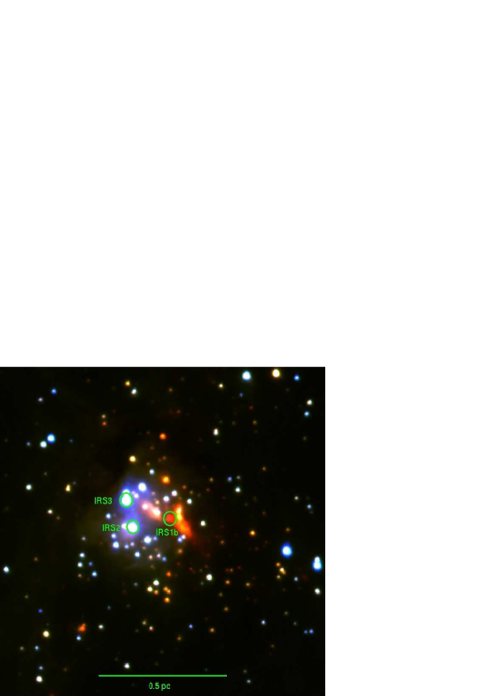
Figure 5: Left panel: $JHK_{\rm s}$ color-composite image of the S255-IR SFR ($J$, blue; $H$, green; and $K_{\rm s}$, red). The FOV is $\sim$ 4^′.9 $\times$ 4^′.9. The box corresponds to the FOV ($\sim$ 1^′.5 $\times$ 1^′.5) of the color-composite image shown in the right panel. Right panel: The enlarged view of the color-composite image of the cluster S255-IR. The ionizing sources of the compact and UC Hii  regions S255-2a, S255-2b and S255-2c (marked with circles), are labeled with IRS3, IRS2 and IRS1b respectively. North is up and east is to the left (see online electronic version for the color images).

Figure 5 represents a false $JHK_{\rm s}$ color-composite image ($J$, blue; $H$, green; and $K_{\rm s}$, red) of our observed region centered on the cluster S255-IR. In Figure 5, a clustering of stellar sources is apparent at the center of the image. The figure also displays several red sources, indicating the presence of likely young stellar population still deeply embedded in the molecular cloud, whereas, bluest stars mainly seen towards the eastern and western parts of the image, are likely evolved/foreground objects of the field. A prominent $K_{\rm s}$-band nebulosity is seen at the center of the cluster, with a dark lane surrounding it. The positions of the ionizing sources are marked with circles in the enlarged version of the color-composite image shown in the right panel of Figure 5, which reveals that most of the red sources in the vicinity of S255-IR lie towards the western side, possibly indicating that more young stars are concentrated in this direction. Apart from the main clustering at the center, patchy nebulosity and diffuse wisp emissions are also seen in the image and many red sources appear to be projected on these emissions. The single dish observations have established the presence of a large column of gas, elongated along the lane between S255 and S257 (Klein et al. 2005). Hence, these red sources are possibly young protostars that are associated with the gas reservoir.

4.1 Nature of the Stellar Sources

We now discuss the nature of the associated low mass stellar population using our NIR observations. To examine the nature of the stellar population in the gas ridge, we used NIR CM ($H-K$/$K$) and CC ($H-K$/$J-H$) diagrams of the sources detected in $HK_{\rm s}$ and $JHK_{\rm s}$ bands, respectively, by comparing with the CM and CC diagrams of a nearby control field. Since the extinction is more sensitive to the shorter wavelength ranges and also young protostars are more prominent at longer wavelengths, we use the sources detected only in $H$ and $K_{\rm s}$ bands to construct $H-K/K$ CM diagrams. Figure 6 shows the CM diagrams for the S255-IR SFR and for the nearby control field, where the nearly vertical solid lines represent ZAMS at a distance of 2.5 kpc, reddened by $A_{V}$ = 0, 2.5, 20, 40 and 60 mag, respectively. The parallel slanting lines represent the reddening vectors to the corresponding spectral type. We would like to mention that the uncertainty in spectral type determination is mainly due to the error in the distance determination as well as the $K_{\rm s}$-band excess of the individual sources. A comparison with the control field reveals that the majority of the cluster population shows an apparent separation from the foreground field stars distributed at ($H-K$) $\sim$ 0.2 mag. Figure 6 manifests that the majority of the sources in the S255-IR region are likely to be reddened MS members and/or pre-main-sequence (PMS) sources with strong infrared excess emission. Most of the sources with $H-K$ $\geq$ 2, not detected in the $J$-band, are likely candidates for young sources with disks and envelopes. Massive stars ($\geq$ 8 $M_{\odot}$) do not have PMS phase and appear on the ZAMS while still embedded in the molecular cloud, whereas, lower mass stars spend a significant amount of time in the PMS phase. Therefore, in Figure $6a$, all the sources may not be reddened ZAMS stars. There are 22 sources in Figure 6 which appear to be massive with spectral type earlier than B3. Probably, these sources appear luminous due to excess emissions in the $K_{\rm s}$-band because one would expect radio free-free emissions in the vicinity of such sources. However, we detected only four compact radio emissions at 14.94 GHz in the vicinity of SFRs S255-IR and S255-N. The map is sensitive down to 0.11 mJy/beam at 14.94 GHz, which corresponds to $\sim$ 2.9 $\times$ 10⁴⁶ number of Lyman continuum photons per second for an optically thin thermal source situated at a distance of 2.5 kpc, for an electron temperature of 10⁴ $K$. This corresponds to a ZAMS spectral type close to B2 (Panagia 1973) and therefore sets an upper limit of $\sim$ 10 $M_{\odot}$, for the sources that do not show compact radio emissions. The sources associated with the radio emissions are marked in the $H-K/K$ CM diagram (Figure 6), following the same nomenclature by Howard et al. (1997). Source IRS3 corresponds to the radio peak S255-2a, the strongest radio continuum source and the bluest of all the stars of the S255-IR cluster. The CM diagram indicates the star as B2 type. The source IRS2 corresponds to the radio peak S255-2b and is situated $\sim$ 2^′′ southwest of S255-2a. The CM diagram suggests the source as B2-B3 type. The infrared spectral type estimation for both the sources is consistent with the radio estimation at 14.94 GHz within a subclass. The position of star IRS1b coincides with the radio source S255-2c and the spectral type of the star appears to be earlier than O5, whereas the radio estimation suggests a spectral type of B1. Since the star shows large $\sim$ $H-K$ color and is not detected in the $J$-band, it is probably the youngest among the three radio sources. The polarization maps by Tamura et al. (1991) at $K$-band show a presence of a dusty disk towards this star. Therefore, we believe that the discrepancy of infrared and radio luminosities is caused by the presence of excess emission in $K_{\rm s}$-band due to the circumstellar disk. We do not discard the possibility of a few reddened background field stars, which might have contaminated the CM diagram. However, by taking into account the distribution of the high column density of ¹³CO molecular gas (Chavarría et al. 2008), it seems unlikely that the stellar sources in the gas ridge consist of significant background contamination.

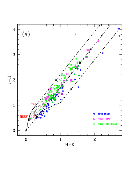
Figure 7: (a) NIR CC diagram of the S255-IR region for the sources detected in the $JHK_{\rm s}$ bands (small dots). The continuous line marks the locus of the MS and thick dashed line is the locus of giant stars. The three parallel dashed lines represent the reddening vectors, the crosses represent a visual extinction of $A_{\rm V}$ = 5 mag. The locus of CTTS is also shown with a dotted line. The positions of the ionizing sources of S255-2a and S255-2b (shown as circles), are labeled with IRS3 and IRS2 respectively. The squares are the IRAC identified Class II and Class I YSOs, whereas the crosses are the IR-excess YSOs identified using NIR plus IRAC bands (for color plot see online electronic version). (b) NIR CC diagram for the control region.

To characterize the different populations of the region, we use the $H-K/J-H$ CC diagram, as shown in Figure 7. The solid thin and thick dashed curves, taken from Bessell & Brett (1988), represent the loci of early MS and late giant stars, respectively. The left and middle parallel dashed lines are the reddening vectors for early MS and late giant stars (drawn from the base and tip of the two branches), respectively. The dotted line represents the locus of classical T Tauri stars (CTTS) (Meyer, Calvet, & Hillenbrand 1997) and the right parallel dashed line represents the reddening vector drawn from the tip of the locus of CTTS. The reddening vectors are plotted using $A_{J}/A_{V}$ = 0.265, $A_{H}/A_{V}$ = 0.155, $A_{K}/A_{V}$ = 0.090 for the CIT system (Cohen et al. 1981). The sources between the left and middle reddening vectors are considered to be either field stars or reddened MS stars or weak-line T Tauri stars, whereas sources with NIR-excess usually fall to the right of the middle reddening vector and are considered as YSOs with disk and envelope (Lada & Adams 1992). The NIR CC diagram can also be contaminated by foreground, background field stars and evolved stars. Therefore, to distinguish the cluster members and YSOs from these objects, we used a statistical approach by comparing the distribution of the sources in the NIR CC diagram of a nearby control region as shown in Figure 7b. Comparison reveals that sources lying between the left and middle reddening vectors with ${\it(J-H)}$ $\geq$ 1.1 and the sources to the right of the middle reddening vectors are likely to be members and YSOs of the region. We do not rule out the possibility that a few massive and intermediate mass members may fall below with ${\it(J-H)}$ $\leq$ 1.1, if they are reddened by the same amount like IRS3 and IRS2. However, considering the initial mass function (IMF) is dominated by the lower mass stars, most of the members should have ${\it(J-H)}$ $\geq$ 1.1 and are possibly reddened MS members or PMS stars with inner circumstellar disk. The evolutionary stages of these sources are difficult to estimate until we know about their SEDs. As can be seen in the CC diagram of the control field, the NIR-excess zone is free of field populations, therefore 83 sources found in the NIR-excess zone in Figure 7$a$ are likely to be YSO candidates. However, this number should be considered as a conservative lower limit, as there are also many sources detected only in $H$ $\&$ $K_{\rm s}$ bands and only in $K_{\rm s}$ band, but not in the $J$ band. The fraction of YSOs increases with high sensitivity observations at $L$- and $M$-band (e.g., Hoffmeister et al. 2008). Spitzer-IRAC observations by Chavarría et al. (2008) uncover several new clusters/groups as well as distributed population of YSOs in the direction of S255-S257 complex. Giving emphasis to the distribution of IRAC classified Class II and Class I sources, they found the ratio of the Class I/Class II sources is highest along the direction of the gas ridge between S255 and S257. In Figure 7$a$, squares represent the distribution of 21 IRAC classified Class I and Class II YSOs and crosses denote the 115 IR-excess YSOs by Chavarría et al. (2008). It is important to note that many sources appear as normal stars in the NIR CC diagram, whereas they show IR-excess in the Spitzer bands. This gives an important clue that many sources that appear likely to be reddened MS stars in the NIR CC diagram, could in reality be PMS sources with disks. In order to discuss the star-formation activity in the gas ridge, we used the spatial distribution of the 83 YSOs identified from the NIR CC diagram and 26 sources having $H-K$ $>$ 2, along with the YSO candidates identified by Chavarría et al. (2008) (see Section 4.4).

4.2 The $K_{\rm s}$-band Luminosity Function

The $K_{\rm s}$-band luminosity function (KLF) of an embedded cluster is useful in constraining the age of the cluster (Megeath et al. 1996; Ojha et al. 2004b,c). In order to derive the observed KLF, one needs to apply corrections for (1) the incompleteness of the star counts as a function of the $K_{\rm s}$ magnitude, and (2) the field star contribution in the line of sight of the cluster. The completeness was determined through artificial star experiments (see Ojha et al. 2004c). To correct for the foreground and background contamination, we used the stellar population synthesis Galactic model (Robin et al. 2003), using a similar procedure described in Ojha et al. (2004c). The star counts were predicted in the direction of S255-IR using the average extinction to the embedded cluster $A_{\rm V}$ = 10 mag for a distance of 2.5 kpc. After the determination of fraction of the contaminating stars over the total model counts, we scaled the model prediction to the star counts in the reference field, and subtracted the foreground and background contamination from the KLF of the S255-IR region.

After correcting for the foreground and background star contamination and photometric completeness, the resulting KLF for the S255-IR region is presented in Figure 8. In Figure 8, a power law with a slope, $\alpha$ [$dN(m_{K})/dm_{K}\propto 10^{\alpha m_{K}}$, where $N(m_{K})$ is the number of stars brighter than $m_{K}$] has been fitted to the KLF using a linear least-squares fitting routine. The KLF of the S255-IR region shows a slope of $\alpha$ = 0.17 $\pm$ 0.03 over the magnitude range 12.5 - 17 in the $K_{\rm s}$-band (solid line in Figure 8). The derived KLF slope is lower than those generally reported for the young embedded clusters ($\alpha\sim 0.4$, e.g., Lada et al. 1991; Lada, Young, & Greene 1993; Lada & Lada 2003), indicating a younger age of $\sim$ 1 Myr. However, a break in the power law can be noticed at $K_{\rm s}$ = 15.25 mag and the KLF seems to be flat in the magnitude range of 15.25 - 17.75. The slope of the KLF in the magnitude range of 12.5 - 15.25 (dashed line in Figure 8) comes out to be 0.25 $\pm$ 0.05 which is still lower than the average value of slopes ($\alpha\sim 0.4$) for young clusters of similar ages (Lada et al. 1991; Lada, Young, & Greene 1993; Lada & Lada 2003). A turn-off in the KLF has also been observed in a few young clusters, e.g. at $K$ $\sim$ 14.5 mag, $K$ $\sim$ 16.0 mag and $K$ $\sim$ 15.75 mag in the case of Tr 14 (distance $\sim$ 2.5 kpc; Sanchawala et al. 2007), NGC 7538 (distance $\sim$ 2.8 kpc; Ojha et al. 2004c) and NGC 1624 (distance $\sim$ 6.0 kpc; Jose et al. 2011), respectively.

4.3 Mass Spectrum of Stellar Sources

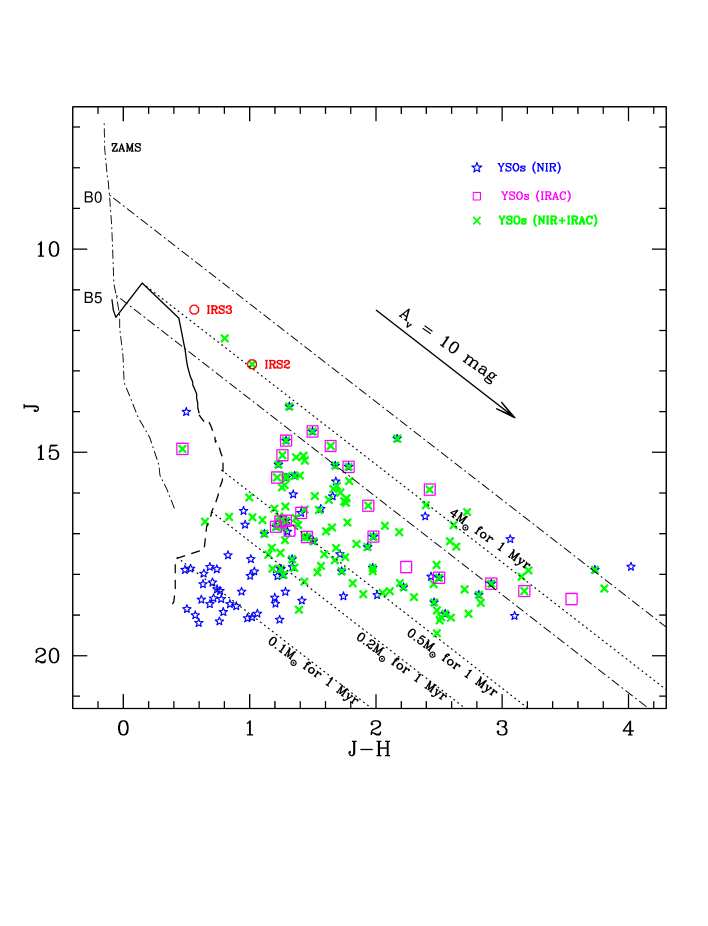
Figure 9: NIR CM diagram for YSOs in the S255 region. The asterisks represent the YSOs, identified on the basis of NIR CC diagram. The squares represent the sources that are identified as YSOs in the IRAC bands, whereas the crosses denote the IR-excess YSOs identified using NIR plus IRAC bands. The PMS isochrones of 1 Myr from Siess et al. (2000) and Baraffe et al. (1998) are drawn in solid and dashed curved lines, respectively, at a distance of 2.5 kpc and zero reddening. The reddening vectors corresponding to 0.1, 0.2, 0.5, and 4 $M_{\odot}$ are also shown in dotted slanting lines. The ZAMS, along with the reddening vectors (dashed-dotted slanting lines) from the tip of B0 and B5 stars are also shown. The ionizing sources of compact and UC Hii regions are marked in the same manner as in Figure 7 (for color plot see online electronic version).

As discussed in Section 4.1, the excess emission in the $K_{\rm s}$-band may make the YSOs luminous, hence the mass estimation on the basis of $H-K/K$ CM diagram will lead to an overestimation of the mass. To minimize the effect of NIR excess emission on mass estimation, we preferred $J$-band luminosity rather than $H$ or $K$ band. Figure 9 represents $J-H/J$ CM diagram for the sources detected in our observed area, where asterisks represent YSOs selected from the NIR $H-K$/$J-H$ CC diagram. We assumed an age of 1 Myr to estimate the mass, which would be appropriate because the mean age of 16 YSOs in the direction of the embedded cluster is found to be $\sim$ 1.2 Myr (see Section 6). The solid and dashed curves in the figure denote the loci of 1 Myr PMS isochrones by Siess et al. (2000) for 1.2 $M_{\odot}$ $\leq$ $M$ $\leq$ 7 $M_{\odot}$ and Baraffe et al. (1998) for 0.05 $M_{\odot}$ $\leq$ $M$ $\leq$ 1.4 $M_{\odot}$, respectively. The dotted slanting lines are the reddening vectors for 4, 0.5, 0.2 and 0.1 $M_{\odot}$ stars for 1 Myr isochrones, respectively. For an assumed age of 1 Myr, the lowest mass detected in our $J$-band image is about 0.1 $M_{\odot}$ for $A_{\rm V}$= 5 mag, and is about 0.3 $M_{\odot}$ for $A_{\rm V}$= 11.5 mag. In Figure 9, squares represent the Spitzer-IRAC identified Class I and Class II YSOs, which indicates that the IRAC observations in the gas ridge are sensitive only down to 0.5 $M_{\odot}$. Whereas the IR-excess YSOs (crosses) identified using NIR plus IRAC bands are sensitive down to 0.2 $M_{\odot}$ for $A_{\rm V}$= 5 mag. The lower sensitivity of IRAC observations are most likely due to the combined effect of saturation, bright polycyclic aromatic hydrocarbon (PAH) emission towards S255-IR region and lower resolution of the IRAC data. Indeed Chavarría et al. (2008) found that the area with PAH emissions in the complex decreases the sensitivity to detect faint sources at 5.8 and 8.0 $\mu$m compared to the area free of PAH emissions. These are the possible causes which might have limited the sensitivity of the IRAC bands to detect YSOs upto 0.5 $M_{\odot}$, less sensitive than our NIR detection ($\sim$ 0.1 $M_{\odot}$). The reddening vectors for the assumed age suggest that most of the YSOs have masses in the range of 0.1 - 4 $M_{\odot}$. With the assumed age, the distribution of YSOs with wide colors (Figure 9) probably indicates the combined effect of variable extinction, weak contribution of excess emission in $J$ and $H$ bands and/or sources in different evolutionary stages (see also Wang et al. 2011). We note that the estimated stellar masses from the infrared CM diagrams rely on the uncertain age and distance. The ambiguity is more severe among the early B-type stars because the inferred stellar mass for a 4 $M_{\odot}$ star from the 1 Myr PMS isochrone can be as high as 18 $M_{\odot}$ when estimated from the MS isochrones of a younger age. For this purpose, we have also drawn the reddening vectors (slanting dashed-dotted lines) from the tip of B0 and B5 ZAMS (dashed-dotted vertical curve) locus. The concept of PMS is not applicable to stars above 8 $M_{\odot}$ since the birth line and the ZAMS unify at those mass levels (Palla & Stahler 1993). Therefore, the ionizing sources IRS3 and IRS2, are likely to be reddened ZAMS massive stars. It is worth pointing out that Howard, Pipher, & Forrest (1997), based on the stellar fit of the observed NIR data points, indicated that the region is rich in B-type stars, containing 9 B0-type ($\sim$ 18 $M_{\odot}$) and 19 B5-type ($\sim$ 6 $M_{\odot}$) MS stars within an area of 1.69 arcmin² centered on S255-IR cluster ($\alpha_{2000}=06^{h}12^{m}53^{s}$, $\delta_{2000}=+17^{\circ}59^{\prime}23^{\prime\prime}$). The $J-H/J$ CM diagram does not reveal such massive members (at least earlier than B0) for an assumed age of 1 Myr, as most of the stars have masses less than 4 $M_{\odot}$. Moreover, one would expect radio emission from such sources. The circumstellar disks are rare among the intermediate mass to massive PMS stars with ages $\sim$ 1 Myr, therefore the mass uncertainty due to the circumstellar disk should not be the major cause for massive members. The discrepancy could be due to the contribution from the bright nebulosity to the photometric magnitudes.

4.4 Spatial Distribution of YSOs

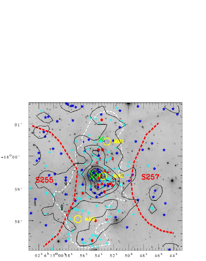
Figure 10: The spatial distributions of YSOs identified using NIR CC diagram (asterisks), sources detected only in $H$ and $K_{s}$ bands with $H-K$ $\geq$ 2 (filled circles) and the sources detected only in the $K_{s}$ band (plus symbols), overlaid on $K_{\rm s}$-band image. The white dashed line shows the outer periphery of the dust continuum emission at 870 $\mu$m, which is at three times of the rms noise (501 mJy/beam) in the sub-milimeter map. The yellow circles are the positions of 1.2 mm continuum cores (MM1, MM2 and MM3; top to bottom) in the gas ridge. The red dashed lines are the demarcation of the outer boundaries of S255 and S257 H ii regions. The large cross signs represent the positions of the radio continuum sources. The YSO SSND contours are shown in black lines. The contour levels are drawn from 20 stars/pc² with an increment of 30 stars/pc². North is up and east is to the left (for color plot see online electronic version).

The infrared excess in the case of YSOs can be due to circumstellar disk/envelope or weaker contribution from the reflected stellar radiation of the dust emission. In any case, infrared excess represents the association of young sources in a SFR and possibly traces the star formation history of a cloud. Figure 10 shows the spatial distribution of YSOs from NIR CC diagram (asterisks), possible YSOs detected only in the $H$ and $K_{\rm s}$ bands with $H-K$ $\geq$ 2 (filled circles) and sources detected only in the $K_{\rm s}$-band (crosses). The outer boundaries of 870 $\mu$m dust continuum emission (Klein et al. 2005) observed with a resolution of $\sim$ 26^′′ are shown with white dashed lines in the figure. This has the shape of a bar extending in the north-south direction and separates the two evolved H ii regions S255 and S257. The outer boundaries of S255 and S257 are also marked with the red thick dashed lines, which are extracted from the ionized gas traced by the radio continuum emission at 610 MHz observed with Giant Metrewave Radio Telescope (GMRT) at a resolution of $\sim$ 5^′′.5 $\times$ 6^′′.5, taken from Zinchenko et al. (in preperation). The yellow circles denote the positions of the three prominent 1.2 mm dust continuum clumps MM1, MM2 and MM3, revealed by Minier et al. (2005) at a resolution of 24^′′. The large crosses represent the positions of the radio continuum sources, three of which are found in the vicinity of the S255-IR cluster and one is associated with the S255N SFR. Most of the NIR YSOs are distributed in the close proximity of the S255-IR cluster and are also projected in the direction of the ionized emissions of the evolved H ii regions. The majority of the YSOs with $H-K$ $\geq$ 2 and those detected only in the $K_{\rm s}$-band are distributed along the bar of dust emission. The sources detected only in the $K_{\rm s}$-band show a scattered distribution along the gas ridge, with an enhanced concentration towards the western side of the S255-IR cluster and in the close vicinity of the molecular clump MM2. Towards S255N, MM1 and MM3, we do not see enhanced concentration of YSOs as seen towards S255-IR, possibly they are in a more embedded phase of star formation. In our observed NIR field, we identified 109 YSO candidates, which include 83 from NIR CC diagram and 26 sources with H-K $>$ 2. Out of 109 sources, we find that only 40 in our observed region are common to the sources classified as YSOs by Chavarría et al. (2008). Therefore, in the present work we identified 69 new YSO candidates in the region. To see the spatial distribution of all the YSO candidates, we overlaid the stellar surface number density (SSND) contour map on the $K_{\rm s}$-band image in Figure 10 using kernel method (Gomez et al. 1993; Silverman 1986). The SSND contour map was made using a total of 213 YSO candidates, which include the 69 new YSOs detected by us and the 144 YSOs found by Chavarría et al. (2008) using NIR and IRAC bands in the region observed by us. The stellar density distribution is smoothened by 0.1 pc $\times$ 0.1 pc sampling box. The contour levels are drawn from 20 stars/pc² with an increment of 30 stars/pc². The clustering towards S255-IR region is obvious in the SSND map along with substructures between S255-IR and MM1 and towards MM2. The main peak of the projected stellar density distribution was found to be $\alpha_{2000}=06^{h}12^{m}53^{s}$, $\delta_{2000}=17^{\circ}59^{\prime}25^{\prime\prime}$, with central density of 180 stars/pc², whereas one can also see a second peak at $\alpha_{2000}=06^{h}12^{m}54^{s}$, $\delta_{2000}=+18^{\circ}00^{\prime}06^{\prime\prime}$, with central density of 87 stars/pc². This distribution confirms the presence of enhanced concentration of YSOs in the gas ridge compared to that towards S255 and S257 and is therefore a relatively more active site of star formation.

5 Stellar Population Beyond the Gas Ridge

So far we have studied the properties of the stellar sources along or in the vicinity of the gas ridge. In order to correlate the star formation activity in the gas ridge with the stellar population beyond the gas ridge, we used the optical CM ($B-V/V$ & $V-I/V$) diagrams for the sources covering a field of $\sim$ 13^′ $\times$ 13^′ centered on S255-IR.

In order to ascertain the age of the stellar members, we attempted quantitative age determination with the help of the optical CM diagram, assuming that the emissions are purely photospheric and contribution from the disks and envelopes in the optical band is negligible. Figure 11 shows $B-V/V$ and $V-I/V$ CM diagrams of all the observed stars. The distribution of the stars in the $B-V/V$ CM diagram resembles the foreground population distribution shown in the $H-K/K$ CM diagram of the control field (see Figure 6b), when constructed using 2MASS PSC. Hence, we presume that a majority of these stars are foreground stars. Moreover, the OB associations are generally not so conspicuous since they extend usually over a large area in the sky and most of the faint stars in the area are actually unrelated foreground or background stars. The identification of the associated faint low-mass members among the field stars is rather difficult. From the $K$-band extinction map, Chavarría et al. (2008) have estimated a lower limit of the extinction value as A_K = 0.4 mag ($A_{\rm V}$ $\sim$ 4.4 mag) for the members of the region. However, it is worth noting that the region shows variable extinction due to non-uniform distribution of the molecular material. In Figure 11 we also plotted the ZAMS by Schmidt-Kaler (1982) using $E(B-V)$ = 1.41 mag (corresponds to $A_{\rm V}$ = 4.4 mag) and $E(V-I)$ = 1.25 $\times$ $E(B-V)$, for a distance of 2.5 kpc. It is worth pointing out that in comparison to $B-V/V$ CM diagram, $V-I/V$ CM diagram has a significant number of stars that fall to the right of reddened ZAMS. These could be low mass Galactic field populations and/or PMS stars of the region. The dynamical ages of the H ii regions S255 and S257 are less than 2 Myr (Chavarría et al. 2008). If we assume that the dynamical ages represent the age of the luminous exciting sources then we would expect a number of contracting low mass PMS stars, because the star formation is a continuous process and the contraction time of the YSOs to reach the MS increases with decrease in mass. For example, the high mass ($>$ 8 $M_{\odot}$) stars take $\sim$ few $\times$ 10⁵ yr to reach the MS, whereas, the low mass YSOs ($\sim$ $1$ $M_{\odot}$) can take 30 Myr to reach the MS. In the absence of proper motion studies and spectroscopic information, the distinction of true low mass members from the contaminating field stars projected along the line of sight is difficult. Therefore, we used the confirmed Class II, Class I and IR-excess YSOs identified by Chavarría et al. (2008). The 51 YSOs having optical counterpart are plotted in the $V-I/V$ CM diagram with circles, triangles and crosses, respectively (see Figure 11). We derived the extinction values of these YSOs by tracing them back along the reddening vector to the CTTS locus or its extension in the $H-K/J-H$ CC diagram. The mean extinction value for the sources above CTTS locus was found to be 4.6 $\pm$ 1.8 mag after excluding those sources that appear below the CTTS locus. These sources are probably reddened Herbig Ae/Be type stars of the region. It is worth noting that the CTTS locus has its own intrinsic broadening due to colors of T-Tauri stars, which could also be a possible reason for the sources that fall below the mean locus. We would like to mention that the approach to estimate the extinction is an approximate one. However, the mean value of $A_{\rm V}$ ($\sim$ 4.6 $\pm$ 1.8 mag) is in agreement with the lower limit of $A_{\rm V}$ ($\sim$ 4.4 mag) suggested by Chavarría et al. (2008).

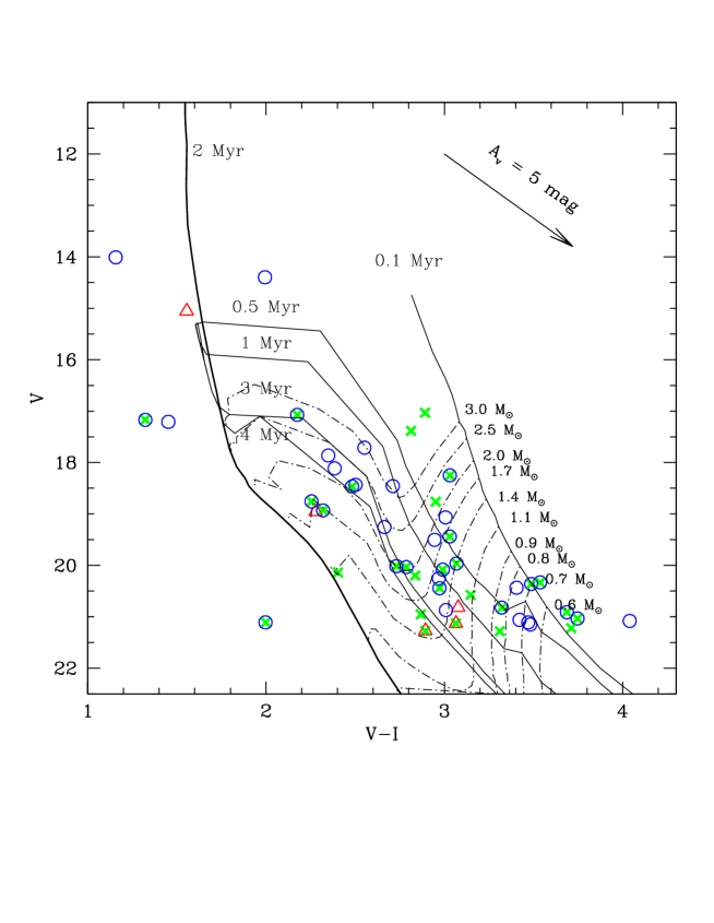
Figure 12: Optical CM diagram for Class II (circles), Class I (triangles) and IR-excess (crosses) YSOs found by Chavarría et al. (2008). The isochrone for 2 Myr age for solar metallicity by Girardi et al. (2002) (thick curve) and PMS isochrones of 0.1, 0.5, 1, 3 and 4 Myr (thin curves) along with evolutionary tracks of different mass (dashed-dotted lines) stars by Siess et al. (2000) are also shown. All the isochrones are corrected for the distance of 2.5 kpc and reddening A_V = 4.6 mag. The arrow indicates a reddening vector for A_V= 5 mag (for color plot see online electronic version).

Figure 12 shows the distribution of YSOs in the $V-I/V$ CM diagram, where the Class II, Class I and IR-excess sources are shown with circles, triangles and crosses, respectively. To estimate the age of the stellar sources, the isochrone for 2 Myr for solar metallicity by Girardi et al. (2002) and PMS isochrones by Siess et al. (2000) for ages of 0.1, 0.5, 1, 3 and 4 Myr have also been plotted. All the isochrones are corrected for a distance of 2.5 kpc and visual extinction of 4.6 mag. The distribution of the PMS stars in the CM diagram implies a span in ages up to 4 Myr. There are a few PMS stars located to the right of 0.1 Myr, these could be highly extincted sources. The age spread could also be an artifact of the combination effects, e.g., variable extinction along the line of sight and variability. However, a similar age spread has been observed in other SFRs as well (e.g., Jose et al. 2008; Sharma et al. 2007). A spectroscopic analysis may lead to a proper estimation of extinction, and a better picture of the age of the stellar sources. To see the mass distribution of PMS stars, we use the grids of evolutionary tracks by Siess et al. (2000), for stellar masses between 0.6 - 3.0 $M_{\odot}$, which are shown with dashed-dotted curved lines in Figure 12. The CM diagram indicates that PMS stars are younger than 4 Myr, with masses between 0.6 to 3.0 $M_{\odot}$. It is to be noted that Spitzer observations reveal that the complex contains several small groups of stellar sources (Chavarría et al. 2008), possibly at different evolutionary stages. Therefore, the observed age spread may represent the mixed population of different ages associated with the molecular cloud. The YSOs included in the optical CM diagram (Fig. 12), are distributed outside of the gas ridge between the two H ii regions S255 and S257, whereas, the YSOs detected in our $JHK_{\rm s}$ bands within the gas ridge are deeply embedded in the molecular cloud of $A_{\rm V}$ $\sim$ 10 mag, and are not detected in the optical bands.

6 Physical Properties of the YSOs

In the previous sections, we have identified YSOs at various locations and discussed their nature with the help of the optical and NIR CM diagrams. In this section, we model the SEDs using the recently available grid of models and fitting tools of Robitaille et al. (2006, 2007). The models are computed using a Monte-Carlo based radiation transfer code (Whitney et al. 2003a,b) using several combinations of central star, disk, in-falling envelope and bipolar cavity for a reasonably large parameter space. The basic model consists of a PMS star surrounded by a flared accretion disk and a rotationally flattened envelope with cavities carved out by a bipolar outflow. Interpreting SEDs using radiative transfer code is subject to degeneracies, and spatially resolved multiwavelength observations can break the degeneracy. Therefore, we only fit the SEDs to those Spitzer-IRAC YSO candidates, for which we have minimum of 6 data points in the wavelength range from 0.55 to 8 $\mu$m, in order to constrain the parameters of stellar photosphere and circumstellar environment. In this approach, we identified 31 sources detected in more than six bands in optical ($VI_{c}$), NIR ($JHK_{\rm s}$) and IRAC (3.6, 4.5, 5.8 & 8.0 $\mu$m) outside the gas ridge and 21 sources having NIR $JHK_{\rm s}$ and IRAC counterparts in the gas ridge. Since the models are valid only for single isolated objects, out of 21 sources in the gas ridge, our $K_{\rm s}$-band image shows presence of multiple sources in 5 cases within the IRAC apertures used by Chavarría et al. (2008) to extract the photometry. Therefore, we fitted SEDs to only 16 isolated sources in the gas ridge. Since the UC Hii regions are not dynamically evolved objects, we also fitted SED to the ionizing source of S255-2c. The SED fitting tool fits each of the models to the data, allowing both the distance and external foreground extinction to be free parameters. We give a distance range of 2.3 to 2.7 kpc (see Section 3) and $A_{V}$ is estimated using the NIR CC diagram. Considering the uncertainties that might have gone into the estimates, we used the estimated value of $A_{V}$ $\pm$ 2 mag as the input parameter. For the massive source associated S255-2c, we estimated $A_{V}$ from $H-K/K$ CM diagram. We further set 10 to 15$\%$ error in NIR and MIR flux estimates due to possible uncertainties in the calibration, extinction and intrinsic object variability. As emphasized by Robitaille et al. (2007), their SED fitting tool does not claim to determine only the set of parameters that provide a good fit to the SED, but it helps to find a range of reasonably well constrained parameters. Adopting a similar approach by Robitaille et al. (2007), we consider only those models to constrain the physical parameters, which satisfy the following equation :

$$\chi^{2}-\chi^{2}_{\rm min}\leq 2N_{\rm data},$$ (1)

where $\chi^{2}_{\rm min}$ is the goodness-of-fit parameter for the best-fit model and $N_{\rm data}$ is the number of input observational data points. Figure 13 shows examples of SEDs with the resulting models for Class II, Class I and ionizing source of the UC Hii region S255-2c. In the figure, a range of models are plotted in solid lines along with the best-fit model. The values of the parameters for the YSOs outside and inside the gas ridge are given in Tables 4 and 5. In the tables, the listed parameters are: the star mass ($M_{\star}$), temperature ($T_{\star}$), stellar age ($t_{\star}$), mass of the disk ($M_{\rm disk}$), disk accretion rate ($\dot{M}_{\rm disk}$), envelope accretion rate ($\dot{M}_{\rm env}$), foreground visual absorption ($A_{V}$) and the $\chi^{2}_{\rm min}$ of the best fit. The tabulated parameters are obtained from the weighted mean and standard deviation of all the models that satisfy Eq. 1, weighted by the inverse square of ${\chi}^{2}$ of each model. The associated errors shown in Tables 4 and 5 are large because we are dealing with a large parameter space, with limited number of observational data points. Additional observational data points from MIR to millimetre wavebands are required to constrain these parameters more precisely. Table 4 reveals that the age of the optically detected YSO candidates varies between 0.5 to 5 Myr, with a mean age of $\sim$ 2.5 Myr, whereas the visual extinction varies from 2.7 to 7.6 mag, with a mean around 4.4 mag. The mass of the YSOs shows a range from 0.9 to 3.0 $M_{\odot}$. These estimations are not distinctly different from the estimation based on the $V-I/V$ diagram. Table 5 shows that the age of the majority of YSOs, along or in the vicinity of the gas ridge, varies from 0.1 to 2 Myr with a mean age of $\sim$ 1.2 Myr, whereas the visual extinction varies form 4.5 to 22.1 mag. The derived cluster age ($\sim$ 2 Myr) is slightly lower than that obtained by Wang et al. (2011) from the intrinsic HR diagram. It is to be noted that the Wang et al. (2011) estimate was determined by adopting a distance of 1.6 kpc. Though direct comparison is not possible because of different approaches to estimate age, it is worth to mention here that adopting a lower distance in the HR diagram makes the age older. The mass of the YSOs shows a range from 0.6 to 7.6 $M_{\odot}$, implying we are sampling YSOs only upto 0.6 $M_{\odot}$. For ionizing source of the UC Hii region S255-2c, the acceptable SED fitting models suggest a massive star ($\sim$ 27 $M_{\odot}$), with an age of $\sim$ 0.1 Myr. The models also predict that the source is deeply embedded behind $\sim$ 42 mag of visual extinction and has an envelope accretion rate of 10^-3.4 yr^-1. Similarly, following the procedure given by Chavarría et al (2008), the dynamical age is estimated to be less than 10⁵ yr for the compact and UC Hii regions, for an assumed density of 10⁵ cm ^-3. These estimations indicate that the massive stars associated with the gas ridge are younger in nature. It is also apparent from Tables 4 and 5 that the disk accretion rate of the YSOs outside the gas ridge is in the range of 10^-7 $-$ 10^-8 $M_{\odot}$ yr^-1, less than that of YSOs in the gas ridge, which is in the range of 10^-6 $-$ 10^-7 $M_{\odot}$ yr^-1. Similarly, the envelope infall rates for most of the YSOs inside the gas ridge are relatively higher than the YSOs outside the gas ridge. These derived characteristics of the YSOs in the gas ridge are possibly the consequence of their younger age than the YSOs distributed outside. However, in the absence of MIR to millimeter data the above values should be treated with caution.

7 Discussion on Star Formation Activity

The derived characteristics of the YSOs along with the morphology of the complex and physical properties of the associated gas and dust can be used to discuss the evolutionary status of the star-forming sites and the overall star-formation activity of the complex.

7.1 Early stage of star formation in the clustered environment

An embedded cluster along with three prominent clumps MM1, MM2 and MM3 (Minier et al. 2005) appear to be sandwiched between the two evolved H ii regions S255 and S257. The clumps MM1 & MM2 contain a similar amount of dense gas of mass $>$ 200 $M_{\odot}$, and show a higher gas temperature of 40 K and are in agreement with that of Zinchenko et al. (2009). This is in contrast to MM3, which has a mass of $\sim$ 100 $M_{\odot}$ and the gas temperature is expected to be around 20 K. These observations led us to suggest that the temperature of MM1 and MM2 is significantly higher than the starless clumps, representing that the clumps are possibly internally heated by the protostars, whereas the clump MM3 represents the earlier stage of star formation as compared to MM1 and MM2. It is to be noted that the clump MM2 lies close to the infrared cluster S255-IR, where the cluster harbors two optically visible massive stars, along with several intermediate to low mass stars of different properties detected in the $JHK_{\rm s}$ bands, whereas, the sources in the vicinity of the clump MM2 are detected in the $K_{\rm s}$-band only, and possibly represent a more embedded phase of star formation. The clump MM2 is also associated with CH₃OH, H₂O and OH masers (Minier et al. 2005; Goddi et al. 2007). CH₃OH maser traces earliest stages of massive star formation (Walsh et al. 1998) and turns off shortly after the formation of UC Hii region. The detection of maser emission towards the centre of MM1, which has a characteristic lifetime of 2.5 $\times$ 10⁴ to 4.5 $\times$ 10⁴ yr (van der Walt 2005), indicates this is not a dynamically evolved object. It seems that the sources associated with the clump MM2 are most probably younger than the sources associated with S255-IR. The sources associated with the H ii regions S255-2a and S255-2b of the cluster S255-IR are not associated with millimetre continuum emission and hence, presumably are in the later stage of evolution. There was also evidence of bipolar outflows from the sources associated with the S255-2c (Wang et al. 2011; Zinchenko et al., in preparation), along with presence of dusty disk (Tamura et al. 1991), which supports the interpretation that the B-type stars may form via an accretion outflow process similar to that of low mass stars. Both these phenomena indicate an early evolutionary stage of the source (IRS1b) associated with S255-2c, which is supported by the dynamical age and the age derived from the SED fitting models (i.e age $\leq$ 0.1 Myr). An interesting question is whether the sources in the vicinity of MM2 and the massive stars of S255-IR have formed in the same region of space. Although presently we do not have the necessary data to address this issue and reach a firm conclusion, it is quite possible that both populations are spatially unrelated. We also do not discard the possibility that they may represent different evolutionary stages of the same cluster forming environment. For example, in the case of the high mass star-forming region, IRAS 20293+3952, Palau et al. (2007) found that the region consists of starless cores, millimeter sources, UC Hii region and more evolved NIR sources. They concluded that these sources are not forming simultaneously in this cluster environment. Rather, there may be different generations of star formation and this could be a possible case for S255-IR. In several cases, as for example W3 (Feigelson & Townsley 2008; Ojha et al. 2009) and IRAS 19343+2026 (Ojha et al. 2010), the massive embedded sources are found to be associated with a cluster of more evolved lower mass Class II and Class III sources, detectable in the NIR bands. This suggests that, in these regions the intermediate to massive protostars have formed after the first generation of low-mass stars. The clump MM1 is associated with an UC Hii region identified in the 14.94 GHz map and is possibly ionized by a B1 type star. Kurtz, Hofner, & Álvarey (2004) detected a Class I CH₃OH maser at 44 GHz and an H₂O maser at 22 GHz in the close vicinity of the UC Hii region. The non-detection of ionizing source(s) of the associated UC Hii region in the near to mid infrared band and the presence of H₂ knots tracing an outflow (Miralles et al. 1997), indicate a very young age. Since the initial phase of massive star formation is intimately linked to cluster formation and the fragmentation of the molecular clouds, this indicate that S255N is a site of cluster formation in its early stage. Indeed, Cyganowski, Brogan, & Hunter (2007) found evidence of a massive protocluster with the help of high resolution ($\sim$ 4^′′.7 $\times$ 2^′′.7) interferometric observations at 1.3 mm continuum emission and detected three compact cores with no infra-red counterparts. The masses of the cores range from 6 - 35 $M_{\odot}$. The identification of centimeter emission and multiple millimeter continuum sources towards the S255N region indicates an ongoing (proto)cluster formation. The features discussed above support the youthfulness of MM2 and MM1 regions and indicate the upper limit for star formation activity around MM2 and MM1 should not be more than $\sim$ 10⁵ yr. The clump MM3 shows no ionized gas emission in the proximity of the dust peak of mass $\sim$ 100 $M_{\odot}$. For a typical star formation efficiency of 0.3 (c.f Lada & Lada 2003), the clump would likely form a star greater than 8 $M_{\odot}$. If this happens then it is a site for the earliest stages of star formation in which the massive star has not yet reached the ZAMS. This indicates that it is likely to be less than $\sim$ 10⁵ years old because a single early B-star (M $\sim$ 10 $M_{\odot}$) reaches the ZAMS in about 10⁵ years. It is worth mentioning that Wang et al. (2011) detected low velocity outflows in MM3 (S255S) as compared to MM2 and MM1 and suggested that MM3 is likely in the collpase phase. The lower temperature of the clump MM3 and non-detection of stellar sources in the $K_{\rm s}$-band possibly indicates that MM3 is in the earliest evolutionary stage. The above discussion reveals that the star formation is non-coeval along the gas ridge, where the stars of ages from 0.1 - 2 Myr are spatially distributed along the different locations of the cloud.

7.2 Surroundings of S255-S257 Complex

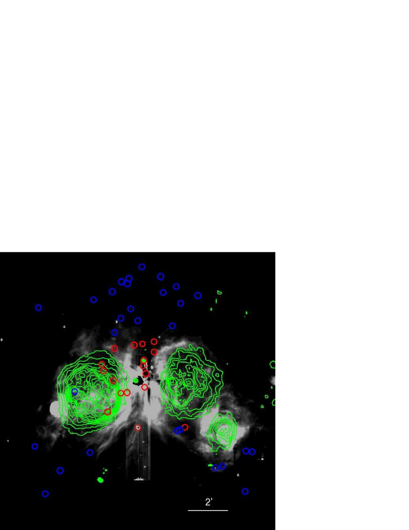
Figure 14: Spatial distribution of sources used for SED fitting, overlaid on the Spitzer IRAC channel 4 (8.0 $\mu$m) image. The green contours represent the 610 MHz emissions taken from Zinchenko et al. (in preparation). The blue circles represent sources with optical counterparts, whereas the red circles are the sources detected in NIR and longer wavelengths (see online electronic version for the color image).

The exciting stars of S255 and S257 are isolated sources, without any co–spatial clustering of low-mass stars around them (Zinnecker et al. 1993). However, Chavarría et al. (2008) hypothesize that a cluster (G192.63-0.00) is associated with S255. Future spectroscopic observations would confirm the association of G192.63-0.00 with S255. Figure 14 shows the surroundings of the evolved H ii regions S255 and S257, where the white background image represents the IRAC 8.0 $\mu$m emissions which generally trace PAHs coming from the photodissociation regions (PDRs) at the surface of the molecular cloud. Generally, these emissions are due to the absorption of far-UV radiation at the surface of the molecular cloud, which escape from the H ii region and the PAHs within PDRs are excited and remit their energy at MIR wavelength. The green radio contours show the ionized gas from radio continuum observations at 610 MHz (Zinchenko et al., in preparation). In radio, both S255 and S257 appear almost circular in size. The figure also displays that 8 $\mu$m emissions are prominent at the peripheries of S255 and S257, in the direction of the dark lane and are weaker towards the interiors of S255 and S257 from the lane, particularly for S257. These emission features correspond to the dark patches seen in the optical band and also roughly coincide with CO emissions found in these directions by Chavarría et al. (2008). The ¹³CO map by Chavarría et al. (2008) reveals that the distribution of the gas is rather non-uniform and clumpy, with its surface density reaching maximum along the gas ridge, where new embedded star formation is expected to occur.

S255-S257 is a part of Gemini OB1 association. The star formation in OB association is often quite complex. One common property of OB associations is that they are sub-structured and often consist of sub-groups of different ages. Carpenter et al. (1995a,b) detected several lower luminosity sources and presumably low mass cores scattered through the Gemini OB1 complex, whereas most of the massive dense cores are found adjacent to the optical H ii regions and often show arc-shaped structure. They interpreted that the induced star formation in the massive dense cores is prominent in the complex due to sweeping and compression of the molecular material. The complex S255-S257 shows a clear congregation of highly obscured YSOs, Herbig-Haro objects, astronomical masers, compact and UC Hii regions. All these sources are concentrated preferentially along the vertical dense bar of gas and dust at the interface of the two H ii regions seen by the ionized gas distribution at 610 MHz. The ionized gas emissions are delineated with PDR, and therefore indicate a definite evidence of physical interaction of the H ii regions with the surrounding molecular material and is responsible for the shaping of the ring like PDR structure. The ionizing sources of the two adjacent evolved H ii regions are MS O9-B0 stars. If they have evolved in the same ambient density, then they might have similar ages. The MS life time of O9 star is of the order of $\sim$ 6.5 Myr. It is difficult to constrain the precise age of the MS star with sufficient accuracy, to compare its relative age with that of the age of YSOs detected in the gas ridge. However, the dynamical age of both the evolved H ii regions is in the range of $\sim$ 0.8-1.6 Myr (Chavarría et al. 2008; Bieging et al. 2009), whereas, the low mass sources scattered in the complex show a mean age of $\sim$ 2.5 Myr. Low mass stars do not dramatically alter the environment in their vicinity, whereas the stellar radiations and winds from massive star(s) play a crucial role in the evolution of the nearby cloud and thus can induce next generation star formation (Elmegreen & Lada 1977). The minimum criteria to ascertain such processes is that the second generation star(s) should have younger age in comparison to nearby massive star(s). The physical properties of the compact and UC Hii  regions in the gas ridge suggest that they are younger than adjacent H ii regions S255 and S257 (see Section 3). The age of the sources inside the dense ridge is of the order of $\sim$ 1.2 Myr or less and considering 1.6 Myr as a typical value for the age of evolved H ii regions, it appears that the sources in the gas ridge are younger than the adjacent massive stars as well as lower mass stars of the complex. These signatures indicate that the sources found in the gas bar might have formed due to the interaction of the evolved H ii regions.

7.3 Triggered Star Formation

A number of mechanisms by which massive stars can affect the subsequent star formation in the region have been proposed. One such process is compression of pre-existing molecular clumps due to impinging of ionization/shock front, leading to density enhancement, which when it exceeds the local critical mass, collapse to form new stars (Bertoldi 1989; Lefloch & Lazareff 1994). The observational signature of such a process would be the limb-brighten rim, having a dense head and a tail, extending away from the ionizing sources (e.g., Miao et al. 2009). The morphology of the radio emissions and/or the H$\alpha$ emission around the sources S255-2a and S255-2b show symmetrical distribution, not like the cometary morphology with a bright rim as found in case of bright-rimmed clouds (e.g. Urquhart et al. 2006; Ogura & Sugitani 1998). The mm contours also do not show any asymmetric distribution of molecular matter, as expected in case of the cometary morphology (e.g. Morgan et al. 2004). The overall distribution of molecular material and the distribution of radio continuum do not give strong evidence in favour of star formation due to compression of pre-existing molecular clumps. However, the compression of pre-existing filamentary cloud cannot be ignored. Another proposed mechanism that can induce star formation around the H ii region is a “collect & collapse” process. In this mechanism, the neutral matter piles up between the ionization and the shock fronts of the expanding H ii region. This compressed material may be dynamically unstable and fragments into dense clumps which can then form new stars (Deharveng et al. 2005). We observed recent star formation activity at the interface of the S255 and S257. If the H ii regions are evolved in the same ambient medium, and S255 is being excited by a relatively early type source, then we expect to have a larger impact on the star formation process at the interface. Therefore, we compare the observed properties with that of the analytical model of star formation at the periphery of the expanding H ii region through “collect and collapse” process by Whitworth et al. (1994). The model predicts the time when the fragmentation starts ($t_{frag}$) and the radius at the time of fragmentation ($R_{frag}$), which weakly depend upon isothermal sound speed in the compressed layer ($a_{s}$), and varies from 0.2 - 0.6 km s^-1, the number of Lyman continuum photons ($Q_{Ly}$) emitted by the massive star and the density of the ambient medium ($n_{0}$) in which the expansion of H ii region occurs and are given by:

$$R_{frag} {\simeq} 5.8~{}a_{.2}^{4/11}~{}Q_{49}^{1/11}~{}n_{3}^{-6/11}~{}pc$$ (2)

$$t_{frag} {\simeq} 1.56~{}a_{.2}^{7/11}~{}Q_{49}^{-1/11}~{}n_{3}^{-5/11}~{}Myr,$$ (3)

where $a_{.2}$=[$a_{s}$/0.2 km s^-1], $Q_{49}$=[$Q_{Ly}$/10⁴⁹ s^-1] and $n_{3}$=[$n_{0}$/10³ cm^-2] are dimensionless variables. Adopting 0.2 km s^-1 for $a_{s}$, 2.4 $\times$ 10⁴⁸ photons s^-1 for $Q_{Ly}$ for the ionizing star (O9.5V) of S255 (Vacca et al. 1996) and 3 $\times$ 10³ for $n_{0}$ (Chavarría et al. 2008 and references therein), we obtained $t_{frag}$ $\approx$ 1.1 Myr and $R_{frag}$ $\approx$ 2.8 pc. This indicates that the fragmentation will start at a radius of 2.8 pc, whereas the young cluster and associated stellar sources are situated at a radius of $\sim$ 1.7 pc from the ionizing star of S255. If one considers the present age of the YSOs ($\sim$ 1.2 Myr) plus the fragmentation time ($\sim$ 1.1 Myr), one would expect an age difference of $>$ 2 Myr between the ionizing source of S255 (age $\sim$ 1.6 Myr) and the YSOs (age $\sim$ 1.2 Myr) in the core. At the same time, to reach from the fragmentation time of the shell to the present age of the YSOs ($\sim$ 1.2 Myr), one would expect a shell radius much beyond 2.8 pc. Though the above estimations are based on the assumptions on the sound speed in the compressed layer. Increasing the value of sound speed increases the fragmentation radius and time further. It appears that the H ii region is not old enough to produce the S255-IR cluster by “collect and collapse” process. Morphologically also, it seems that “collect and collapse” process is not viable here, as the cluster S255-IR is not associated with the ring of PAH emissions that surround the H ii regions S255 or S257, which generally represent the compressed neutral matter piled up between the ionization and shock fronts. Rather, the cluster is situated at the tip of the ring of PAH emissions. For example, in the case of a sample of H ii regions by Deharveng et al. (2005), where the star formation at their peripheries is expected due to “collect and collapse” process, one can see young sources/condensations, which are associated with the ring of PAH emissions that delineate the H ii regions. Also in an ideal case, one would expect regularly spaced clumps along the periphery of H ii regions and/or young protostars of roughly similar ages, distributed preferentially along the swept-up material, which is not the case here, whereas we are seeing sources at different evolutionary stages across the gas ridge and dense clumps. The radio emission from S255 and S257 at 610 MHz is rather spherical and does not show morphology similar to the Champagne flow or blister type H ii regions, where one would expect the evolution of the H ii region in a non-uniform medium. As a result, clump formation due to “collect and collapse” process may not be uniformly distributed. This discussion indicates that the “collect and collapse” process is also not at work here.

In the gas ridge which scenario should work better is difficult to conclude, but the existence of molecular clumps is not unique to the “collect & collapse” model. Moreover, in this process the clumps should be distributed in a ring like structure in the immediate H ii regions, not like the vertical bar structure which we are witnessing here. The morphological similarity of the matter sandwiched between S255-S257 resembles on a large scale the process of star formation that has been observed in the dense bar like structure in the Large Magellanic Cloud at the interfaces of two expanding supergiant shells LMC4 and LMC5 (Cohen et al. 2003), where it is believed that the collisions between the dense swept up neutral materials lead to star formation (Yamaguchi et al. 2001a,b). This similar kind of star formation activity might have happened here. The above discussion reveals that it is difficult to constrain a particular scenario that is at work with the present analysis, though we favour the last scenario. However, to strengthen the notion that the RDI and “collect & collapse” scenarios are not at work, it would be very useful to get radial velocity information and the age of the stellar members using spectroscopic observations to confirm their association and relative evolutionary status, in order to obtain a better picture of triggered star formation.

8 Conclusions

1. Deep $JHK_{\rm s}$ observations have been carried out in a region of 4^′.9 $\times$ 4^′.9 centered on the S255-IR cluster associated with the gas ridge between two evolved H ii regions S255 and S257. Using the NIR CC and CM diagrams as main diagnostics of the PMS nature of the objects, we identified 109 likely YSO candidates to a mass limit of 0.1 $M_{\odot}$, which include 69 new YSO candidates in the region observed by us. Our observations increased the number of previously identified YSOs in this region by 32%.

2. Using $J-H/J$ CM diagram and assuming an age of 1 Myr, we found that the masses of the YSOs are in the range of 0.1 - 4 $M_{\odot}$  and they are embedded in the molecular cloud (mean $A_{\rm V}$ $\sim$ 10 mag).

3. Throughout the observed region, the distribution of YSOs with excess emission is not uniform and is more concentrated along the gas ridge found at the interface of the two H ii regions S255 and S257. The YSO surface number density is found to be maximum ($\sim$ 180 stars/pc²) towards the cluster S255-IR, however one can also see sub-structures in the map, with a secondary peak ($\sim$ 87 stars/pc²) towards the northern side of the S255-IR.

4. Out of three massive (M $\geq$ 100 $M_{\odot}$) dust continuum clumps along the gas ridge, we observed radio continuum emission in two clumps. The physical properties of the radio emission are similar to those of compact and UC Hii regions, in agreement with previous observations. The spectral types estimated from the Lyman continuum photons suggest that they are powered by massive B1-B2 type of stars. We suggest that massive star formation has started in two clumps and the massive young sources (IRS 1-3 and S255N) are at different evolutionary stages and are probably younger than the low mass YSOs of the region.

5. The slope of the KLF in the gas ridge is found to be 0.17 $\pm$ 0.03, which is similar to that obtained for young clusters and indicates a young age of $<$ 1 Myr for the stellar sources. However, there is an indication of a break in the power law at $K_{\rm s}$ = 15.25 mag. The KLF slope in the magnitude range of 12.5 - 15.25 can be represented by $\alpha$ = 0.25 $\pm$ 0.05 and the KLF slope is found to be flat in the magnitude range of 15.25 - 17.75.

6. We constucted $V-I/V$ CM diagram of the YSOs (distributed outside the gas ridge) identified on the basis of NIR and IRAC observations. The positions of these YSOs in the CM diagram indicate approximate age between 0.1 - 4 Myr, suggesting a possibility of non-coeval star formation in the S255-S257 complex.

7. The evolutionary status of 31 YSO candidates located outside the gas ridge and 16 YSO candidates located within the gas ridge has been studied using the SED fitting models. The models predict that the mean age of the YSO candidates outside the gas ridge is $\sim$ 2.5 Myr, accreting with disk accretion rate in the range of 10^-7 $-$ 10^-8 $M_{\odot}$ yr^-1, while the mean age of the YSO candidates inside the gas ridge is $\sim$ 1.2 Myr, accreting with disk accretion rate in the range of 10^-6 $-$ 10^-7 $M_{\odot}$ yr^-1. This indicates that the YSOs inside the gas ridge are younger than those outside the gas ridge.

8. We find that the morphology of the molecular material and the distribution of YSOs at the interface of two optically visible evolved H ii regions, resembles, on a large scale, the star formation that has been observed at the interfaces of two supergiant bubbles LMC4 and LMC5, where it is believed that the star formation has occurred due to the collision of the swept up material by the bubbles. Hence, we believe this may be the site of induced star formation as found in the case of LMC4 and LMC5.

Table 1: Log of observational data

Date (UT)	Object	Filter	No of	Exp (sec)	Telescope
			frames	per frame
2004 Dec 15	S255/257	B	3	600	ST
2004 Dec 15		V	3	600	ST
2004 Dec 15		Ic	3	600	ST
2005 Oct 10		H${\alpha}$	1	900	ST
2009 Oct 14	S255/257	B	2	200	ST
2009 Oct 14		V	2	150	ST
2009 Oct 14		Ic	2	60	ST
2009 Oct 14	SA98	B	3	600	ST
2009 Oct 14		V	3	600	ST
2009 Oct 14		Ic	3	100	ST
2008 Jan 11	S255	IFOSC7	1	1200	IGO
2008 Jan 11	S257	IFOSC7	1	1200	IGO
2009 Dec 20	S255-2a	Gr 7	1	1800	HCT
2010 Jan 18	S255-2b	Gr 7	1	2400	HCT
2000 Oct 13	S255-IR	J	18	20	UH
2000 Oct 13		H	18	20	UH
2000 Oct 13		K	18	20	UH

Table 2: Observed integrated flux and angular size for associated H ii regions at 14.94 GHz

Source	Peak Position		Int. Flux	Angular Size
	$\alpha$(J2000)	$\delta$(J2000)	mJy
S255-2a	06:12:55.02	+17:59:29.06	3.307	5′′.9 $\times$ 3′′.9
S255-2b	06:12:54.91	+17:59:21.21	1.620	3′′.0 $\times$ 2′′.7
S255-2c	06:12:54.08	+17:59:24.20	3.060	3′′.2 $\times$ 1′′.3
S255-N	06:12:53.52	+18:00:26.16	9.259	2′′.5 $\times$ 1′′.4

Table 3: Derived physical parameters for the H ii regions from radio observations

Source	$\tau_{c}$	rms $n_{e}$	EM	log NLyc	ZAMS${\dagger}$
		(103 cm-3)	(106 cm-6 pc)	(ph. s-1)	Spectral type
S255-2a	0.0002	1.627	1.545	45.11	B1
S255-2b	0.0002	2.522	2.185	44.77	B2
S255-2c	0.0009	5.637	7.891	45.07	B1
S255-N	0.003	11.210	28.555	45.55	B1

Table 4: Inferred physical parameters of the YSOs detected outside the gas ridge from SED fits

ID	RA	DEC	M∗	T∗	t∗	Mdisk	$\dot{M}_{\rm disk}$	$\dot{M}_{\rm env}$	AV	$\chi^{2}_{\rm min}$
	(J2000)	(J2000)	($M_{\odot}$)	(104 K)	(106 yr)	( $M_{\odot}$)	(10-8 $M_{\odot}$/yr)	(10-6 $M_{\odot}$/yr )	mag
1	93.309601	17.895531	2.089 $\pm$ 0.522	7.642 $\pm$ 2.087	5.058 $\pm$ 2.919	0.005 $\pm$ 0.011	3.305 $\pm$ 3.065	0.233 $\pm$ 1.731	4.418 $\pm$ 1.022	3.78
2	93.296382	17.914910	2.023 $\pm$ 0.526	5.031 $\pm$ 0.620	2.076 $\pm$ 1.985	0.011 $\pm$ 0.017	2.761 $\pm$ 2.523	0.235 $\pm$ 0.744	3.017 $\pm$ 0.449	3.68
3	93.269846	17.930154	1.161 $\pm$ 0.562	4.349 $\pm$ 0.519	2.082 $\pm$ 1.830	0.003 $\pm$ 0.007	0.676 $\pm$ 0.646	2.234 $\pm$ 51.020	4.103 $\pm$ 0.856	9.62
4	93.248081	18.017855	2.544 $\pm$ 0.745	7.392 $\pm$ 2.437	3.671 $\pm$ 2.335	0.011 $\pm$ 0.027	8.455 $\pm$ 7.998	2.523 $\pm$ 11.920	6.701 $\pm$ 1.297	6.29
5	93.248309	18.031191	2.962 $\pm$ 0.818	9.344 $\pm$ 3.698	3.916 $\pm$ 2.449	0.010 $\pm$ 0.023	6.824 $\pm$ 6.509	3.625 $\pm$ 30.850	6.100 $\pm$ 1.084	4.75
6	93.242913	18.043001	2.396 $\pm$ 0.478	5.454 $\pm$ 1.749	1.281 $\pm$ 1.040	0.002 $\pm$ 0.007	0.468 $\pm$ 0.461	0.488 $\pm$ 1.667	3.110 $\pm$ 0.736	7.81
7	93.242141	18.073953	0.931 $\pm$ 0.471	4.170 $\pm$ 0.329	1.446 $\pm$ 0.757	0.001 $\pm$ 0.003	0.132 $\pm$ 0.161	2.134 $\pm$ 45.570	3.054 $\pm$ 0.549	3.40
8	93.233942	18.051073	2.968 $\pm$ 0.664	9.488 $\pm$ 2.604	4.572 $\pm$ 2.942	0.010 $\pm$ 0.032	7.818 $\pm$ 8.602	7.459 $\pm$ 38.170	6.374 $\pm$ 1.138	4.82
9	93.223580	18.021441	3.011 $\pm$ 0.615	11.250 $\pm$ 2.263	5.765 $\pm$ 2.013	0.002 $\pm$ 0.007	2.169 $\pm$ 2.493	0.005 $\pm$ 0.077	7.262 $\pm$ 0.624	1.57
10	93.227723	18.041165	1.871 $\pm$ 0.583	5.759 $\pm$ 1.848	3.599 $\pm$ 3.067	0.007 $\pm$ 0.013	2.584 $\pm$ 2.511	0.537 $\pm$ 4.343	4.763 $\pm$ 0.940	5.36
11	93.235539	18.076643	1.504 $\pm$ 0.424	4.723 $\pm$ 0.479	3.042 $\pm$ 2.250	0.004 $\pm$ 0.008	0.422 $\pm$ 0.398	1.186 $\pm$ 39.370	3.734 $\pm$ 0.542	5.84
12	93.192612	17.948321	1.748 $\pm$ 0.777	4.567 $\pm$ 0.491	0.707 $\pm$ 0.704	0.006 $\pm$ 0.014	1.571 $\pm$ 1.485	2.725 $\pm$ 14.350	3.390 $\pm$ 0.624	4.79
13	93.224064	18.086501	1.571 $\pm$ 0.493	4.970 $\pm$ 1.479	2.363 $\pm$ 1.938	0.001 $\pm$ 0.003	0.036 $\pm$ 0.047	0.583 $\pm$ 24.560	3.195 $\pm$ 0.872	2.42
14	93.190166	17.949554	1.216 $\pm$ 0.700	4.257 $\pm$ 0.442	0.622 $\pm$ 0.589	0.003 $\pm$ 0.008	0.761 $\pm$ 0.740	3.769 $\pm$ 13.420	4.099 $\pm$ 0.974	3.85
15	93.197295	18.036892	1.887 $\pm$ 0.658	4.721 $\pm$ 0.478	1.218 $\pm$ 1.014	0.001 $\pm$ 0.004	0.134 $\pm$ 0.144	0.929 $\pm$ 12.690	3.548 $\pm$ 0.683	6.77
16	93.193666	18.069832	2.044 $\pm$ 0.547	5.626 $\pm$ 2.224	2.218 $\pm$ 2.251	0.001 $\pm$ 0.004	0.446 $\pm$ 0.550	0.158 $\pm$ 0.946	3.115 $\pm$ 0.915	5.33
17	93.283778	17.981431	2.186 $\pm$ 0.983	5.235 $\pm$ 1.119	1.963 $\pm$ 2.030	0.022 $\pm$ 0.029	22.700 $\pm$ 21.050	8.179 $\pm$ 31.220	6.318 $\pm$ 0.902	5.02
18	93.266869	18.058787	1.789 $\pm$ 0.545	5.119 $\pm$ 1.401	2.315 $\pm$ 2.069	0.001 $\pm$ 0.007	0.160 $\pm$ 0.163	0.488 $\pm$ 11.720	2.702 $\pm$ 0.857	7.70
19	93.250234	18.065654	1.155 $\pm$ 0.520	4.357 $\pm$ 0.492	2.132 $\pm$ 1.771	0.003 $\pm$ 0.006	0.536 $\pm$ 0.503	1.430 $\pm$ 40.350	4.100 $\pm$ 0.811	2.75
20	93.236915	18.072354	1.157 $\pm$ 0.439	4.415 $\pm$ 0.504	2.911 $\pm$ 2.463	0.003 $\pm$ 0.005	0.623 $\pm$ 0.589	0.130 $\pm$ 1.057	3.701 $\pm$ 0.706	7.67
21	93.207396	18.078301	1.922 $\pm$ 0.638	5.837 $\pm$ 1.864	3.756 $\pm$ 3.162	0.007 $\pm$ 0.014	2.872 $\pm$ 2.699	1.231 $\pm$ 8.120	4.845 $\pm$ 1.100	5.13
22	93.158847	17.917292	2.593 $\pm$ 1.016	4.870 $\pm$ 0.927	0.466 $\pm$ 0.530	0.026 $\pm$ 0.035	22.490 $\pm$ 20.780	51.130 $\pm$ 125.800	4.292 $\pm$ 1.122	3.17
23	93.189721	18.055715	1.635 $\pm$ 0.332	4.946 $\pm$ 0.765	3.767 $\pm$ 2.472	0.005 $\pm$ 0.009	0.490 $\pm$ 0.451	0.032 $\pm$ 0.738	3.029 $\pm$ 0.473	2.35
24	93.152634	17.918401	2.797 $\pm$ 0.744	5.005 $\pm$ 0.589	0.775 $\pm$ 0.664	0.028 $\pm$ 0.041	10.700 $\pm$ 10.080	8.291 $\pm$ 35.320	5.701 $\pm$ 1.271	5.53
25	93.131845	17.931312	1.345 $\pm$ 0.758	4.421 $\pm$ 0.579	1.505 $\pm$ 1.314	0.005 $\pm$ 0.008	1.231 $\pm$ 1.159	1.389 $\pm$ 10.260	4.468 $\pm$ 1.066	4.62
26	93.315675	18.051981	1.686 $\pm$ 0.525	4.716 $\pm$ 0.457	1.823 $\pm$ 1.501	0.001 $\pm$ 0.005	0.144 $\pm$ 0.153	0.756 $\pm$ 14.140	3.591 $\pm$ 0.654	6.53
27	93.205126	18.064643	2.227 $\pm$ 0.603	7.665 $\pm$ 2.379	4.900 $\pm$ 2.760	0.010 $\pm$ 0.017	7.030 $\pm$ 6.758	3.788 $\pm$ 28.590	6.289 $\pm$ 1.184	1.77
28	93.126392	17.930826	2.996 $\pm$ 0.886	6.156 $\pm$ 1.675	2.112 $\pm$ 2.108	0.015 $\pm$ 0.023	6.593 $\pm$ 6.322	5.581 $\pm$ 22.520	4.009 $\pm$ 1.268	13.66
29	93.318921	17.935201	2.523 $\pm$ 0.782	4.918 $\pm$ 0.487	0.984 $\pm$ 0.674	0.003 $\pm$ 0.007	0.433 $\pm$ 0.417	2.171 $\pm$ 9.788	6.622 $\pm$ 0.847	7.73
30	93.174703	18.062276	1.487 $\pm$ 0.439	4.732 $\pm$ 0.468	3.549 $\pm$ 2.524	0.005 $\pm$ 0.009	0.770 $\pm$ 0.722	0.159 $\pm$ 2.644	3.599 $\pm$ 0.618	5.38
31	93.132735	17.897481	2.939 $\pm$ 0.520	8.590 $\pm$ 2.235	2.630 $\pm$ 1.010	0.008 $\pm$ 0.025	11.320 $\pm$ 10.910	1.551 $\pm$ 13.240	4.397 $\pm$ 0.623	2.92

Table 5: Inferred physical parameters of the YSOs detected inside the gas ridge from SED fits

ID	RA	DEC	M∗	T∗	t∗	Mdisk	$\dot{M}_{\rm disk}$	$\dot{M}_{\rm env}$	AV	$\chi^{2}_{\rm min}$
	(J2000)	(J2000)	($M_{\odot}$)	(104 K)	(106 yr)	( $M_{\odot}$)	(10-8 $M_{\odot}$/yr)	(10-6 $M_{\odot}$/yr )	mag
1	93.186031	17.951481	0.720 $\pm$ 0.775	3.687 $\pm$ 0.725	1.392 $\pm$ 2.219	0.006 $\pm$ 0.013	5.980 $\pm$ 7.953	17.490 $\pm$ 88.960	5.561 $\pm$ 1.291	1.69
2	93.254402	17.964297	1.987 $\pm$ 1.512	4.789 $\pm$ 1.812	0.670 $\pm$ 1.600	0.021 $\pm$ 0.052	18.750 $\pm$ 18.700	19.080 $\pm$ 33.470	7.314 $\pm$ 1.114	3.11
3	93.242582	17.980096	3.085 $\pm$ 0.819	5.541 $\pm$ 0.706	1.188 $\pm$ 0.620	0.007 $\pm$ 0.016	1.568 $\pm$ 1.430	27.540 $\pm$ 92.210	9.688 $\pm$ 1.637	2.71
4	93.237271	17.980611	3.131 $\pm$ 1.259	5.468 $\pm$ 2.361	0.751 $\pm$ 1.866	0.050 $\pm$ 0.079	120.200 $\pm$ 105.800	84.480 $\pm$ 197.000	13.660 $\pm$ 2.390	1.89
5	93.221573	17.984965	3.024 $\pm$ 1.152	5.435 $\pm$ 1.501	0.974 $\pm$ 1.195	0.026 $\pm$ 0.036	78.710 $\pm$ 72.440	20.010 $\pm$ 55.650	10.690 $\pm$ 1.938	4.54
6	93.249381	17.990787	1.236 $\pm$ 1.549	3.770 $\pm$ 0.716	0.744 $\pm$ 2.004	0.015 $\pm$ 0.041	36.180 $\pm$ 32.790	45.550 $\pm$ 134.000	4.519 $\pm$ 1.232	1.67
7	93.258103	17.998671	0.950 $\pm$ 0.879	4.021 $\pm$ 1.020	1.040 $\pm$ 1.873	0.007 $\pm$ 0.010	5.771 $\pm$ 5.241	8.943 $\pm$ 25.210	6.680 $\pm$ 1.622	3.30
8	93.222334	18.007723	7.690 $\pm$ 1.621	8.597 $\pm$ 4.189	0.199 $\pm$ 0.215	0.200 $\pm$ 0.339	376.800 $\pm$ 364.100	490.600 $\pm$ 470.200	6.678 $\pm$ 2.994	21.37
9	93.248134	18.017854	2.537 $\pm$ 0.602	7.599 $\pm$ 2.309	4.045 $\pm$ 2.705	0.015 $\pm$ 0.026	6.645 $\pm$ 6.236	2.594 $\pm$ 17.380	6.067 $\pm$ 1.379	3.81
10	93.231215	18.020677	1.806 $\pm$ 1.014	5.177 $\pm$ 1.952	1.797 $\pm$ 2.277	0.020 $\pm$ 0.022	27.530 $\pm$ 23.120	11.000 $\pm$ 35.700	5.791 $\pm$ 1.641	1.43
11	93.223622	18.021473	2.620 $\pm$ 0.990	6.463 $\pm$ 3.343	1.500 $\pm$ 2.165	0.010 $\pm$ 0.022	3.900 $\pm$ 3.650	9.623 $\pm$ 31.410	7.729 $\pm$ 1.217	3.85
12	93.213193	18.023401	0.657 $\pm$ 0.835	3.588 $\pm$ 1.041	0.787 $\pm$ 1.593	0.010 $\pm$ 0.022	10.920 $\pm$ 9.546	11.540 $\pm$ 42.730	5.333 $\pm$ 1.151	1.66
13	93.222891	18.003234	3.636 $\pm$ 0.959	10.110 $\pm$ 4.614	2.773 $\pm$ 2.665	0.015 $\pm$ 0.034	11.770 $\pm$ 11.330	16.330 $\pm$ 60.620	22.140 $\pm$ 2.431	2.08
14	93.259425	18.004278	1.175 $\pm$ 0.848	4.310 $\pm$ 1.007	1.183 $\pm$ 1.949	0.007 $\pm$ 0.011	6.775 $\pm$ 6.645	11.070 $\pm$ 32.760	5.208 $\pm$ 1.573	2.85
15	93.213312	18.014792	1.193 $\pm$ 1.341	4.194 $\pm$ 1.560	0.321 $\pm$ 1.316	0.014 $\pm$ 0.032	35.600 $\pm$ 42.540	15.450 $\pm$ 24.570	5.882 $\pm$ 1.219	1.05
16	93.220701	17.996683	1.943 $\pm$ 1.640	4.210 $\pm$ 0.337	0.096 $\pm$ 0.097	0.025 $\pm$ 0.064	31.580 $\pm$ 27.180	26.820 $\pm$ 21.810	9.245 $\pm$ 1.380	1.50

Figure 2: Comparison of UH/SIRIUS $JHK_{\rm s}$ photometry with the 2MASS data for the common sources. The difference $\Delta$ (UH - 2MASS) in mag is plotted as a function of $J$ mag.

Figure 3: The blue part of the spectra of the ionizing sources of the H ii regions. Spectra are normalised and shifted with arbitrary units.

.

Figure 6: (a) NIR CM diagram of the S255-IR SFR. The vertical solid lines from left to right indicate the MS track at 2.5 kpc reddened by $A_{\rm V}$= 0, 2.5, 20, 40, and 60 mag, respectively. Slanting horizontal lines represent the standard reddening vectors drawn from the MS locus corresponding to different spectral types. The positions of the ionizing sources of S255-2a, S255-2b and S255-2c (shown as circles), are labeled with IRS3, IRS2 and IRS1b respectively. (b) NIR CM diagram for the control region.

Figure 8: The completeness-corrected and field star-subtracted KLF of the S255-IR region. The linear fits for various magnitude ranges are represented by the straight lines (see the text).

Figure 11: The CM diagrams for stars lying in the S255-S257 cluster region. The dashed curve represents ZAMS by Schmidt-Kaler (1982) corrected for $E(B-V)$ = 1.41 mag ($A_{\rm V}$ = 4.4 mag) and distance of 2.5 kpc. The Class II (circles), Class I (triangles) and IR-excess (crosses) YSOs identified by Chavarría et al. (2008) are also marked.

Figure 13: The SEDs of IRAC identified YSOs with optical and NIR counterparts outside the gas ridge (left), only NIR counterparts inside the gas ridge (middle) and the YSO associated with UC Hii  region S255-2c (right). The solid lines show the family of models that fit the data reasonably with ${\chi}^{2}-{\chi^{2}_{\rm min}}\leq 2N_{\rm data}$, where ${\chi}^{2}_{\rm min}$ is the goodness-of-fit parameter for the best-fit model (see the text). The dashed line shows the SED of the stellar photosphere in the best-fitting model. The filled circles denote the input flux values (for color plot see online electronic version).

References

- Baraffe et al. (1998) Baraffe, I., Chabrier, G., Allard, F., & Hauschildt, P. H. 1998, A&A, 337, 403
- Bertoldi (1989) Bertoldi, F. 1989, ApJ, 346, 735
- Bessell & Brett (1988) Bessell, M. S. & Brett, J. M. 1988, PASP, 100, 1134
- Bieging et al. (2009) Bieging, J. H., Peters, W. L., Vila Vilaro, B., Schlottman, K., & Kulesa, C. 2009, AJ, 138, 975
- Carpenter (1995) Carpenter, J. M., Snell, R. L., & Schloerb, F. P. 1995a, ApJ, 450, 201
- Carpenter (1995) Carpenter, J. M., Snell, R. L., & Schloerb, F. P. 1995b, ApJ, 445, 246
- Chavarría et al. (2008) Chavarría, L. A., Allen, L. E., Hora, J. L., Brunt, C. M., & Fazio, G. G. 2008, ApJ, 682, 445
- Cohen (1981) Cohen, J. G., Persson, S. E., Elias, J. H., & Frogel, J. A. 1981, ApJ, 249, 481
- Cohen (2003) Cohen, M., Staveley-Smith, L., & Green, A. 2003, MNRAS, 340, 275
- Cox (2000) Cox, A.N. 2000, Allen’s Astrophysical Quantities, Fourth edition (New York: AIP Press; Springer), ed. Arthur N. Cox Point Sources (Pasadena: NASA / IPAC), http://irsa.ipac.caltech.edu/applications/Gator
- Cyganowski et al. (2007) Cyganowski, C. J., Brogan, C. L., & Hunter, T. R. 2007, AJ, 134, 346
- Deharveng et al. (2005) Deharveng, L., Zavagno, A., & Caplan, J. 2005, A&A, 433, 565
- Elmegreen & Lada (1977) Elmegreen, B. G., & Lada, C. J. 1977, ApJ, 214, 725
- Feigelson et al. (2008) Feigelson, E. D., & Townsley, L. K. 2008, ApJ, 673, 354
- Girardi et al. (2002) Girardi, L., Bertelli, G., Bressan, A., et al. 2002, A&A, 391, 195
- Goddi et al. (1989) Goddi, C., Moscadelli, L., Sanna, A., Cesaroni, R., & Minier, V. 2007, A&A, 461, 1027
- Gomez et al. (1989) Gomez, M., Hartmann, L., Kenyon, S. J., & Hewett, R. 1993, AJ, 105, 1927
- Heyer et al. (1989) Heyer, M. H., Snell, R. L., Morgan, J., & Schloerb, F. P. 1989, ApJ, 346, 220
- Hoffmeister et al. (2008) Hoffmeister, V. H., Chini, R., Scheyda, C. M., et al. 2008, ApJ, 686, 310
- Howard et al. (1997) Howard, E. M., Pipher, J. L., & Forrest, W. J. 1997, ApJ, 481, 327
- Huang et al. (1986) Huang, Y. -L., & Thaddeus, P. 1986, ApJ, 309, 804
- Jaffe et al. (1984) Jaffe, D. T., Davidson, J. A., Dragovan, M., & Hildebrand, R. H. 1984, ApJ, 284, 637
- Jose et al. (2008) Jose, J., Pandey, A. K., Ojha, D.K., et al. 2008, MNRAS, 384, 1675
- Jose et al. (2011) Jose, J., Pandey, A. K., Ogura, K., et al. 2011, MNRAS, 411, 2530
- Klein et al. (2008) Klein, R., Posselt, B., Schreyer, K., Forbrich, J., & Henning, Th. 2005, ApJS, 161, 361
- Kurtz et al. (1994) Kurtz, S., Churchwell, E., & Wood, D. O. S. 1994, ApJS, 91, 659
- Kurtz, Hofner, & Álvarez (2004) Kurtz, S., Hofner, P., & Álvarez, C. V. 2004, ApJS, 155, 149
- Kurtz et al. (2000) Kurtz, S., Cesaroni, R., Churchwell, E., Hofner, P., & Walmsley, C. M. 2000, in Protostars and Planets IV, eds. V. Mannings, A. P. Boss, & S. S. Russell (Tucson, AZ: Univ. Arizona Press), pp 299
- Lada et al. (1991) Lada, E. A., Depoy, D. L., Evans, N. J., & Gatley, I. 1991, ApJ, 371, 171
- Lada & Adams (1992) Lada, C. J., & Adams, F. C. 1992, ApJ, 393, 278
- Lada et al. (1993) Lada, C. J., Young, E. T., & Greene, T. P. 1993, ApJ, 408, 471
- Lada & Lada (2003) Lada, C. J., & Lada, E. A. 2003, ARA&A, 41, 57
- Landolt (1992) Landolt, A. U. 1992, AJ, 104, 340
- Lefloch & Lazareff (1994) Lefloch, B., & Lazareff, B. 1994, A&A, 289, 559
- Megeath et al. (1996) Megeath, S. T., Herter, T., Beichman, C., et al. 1996, A&A, 307, 775
- Meyer et al. (1997) Meyer, M. R., Calvet, N., & Hillenbrand, L. A. 1997, AJ, 114, 288
- Meynet et al. (1994) Meynet, G., Maeder, A., Schaller, G., Schaerer, D., & Charbonnel, C. 1994, A&AS, 103, 97
- Mezger et al. (1997) Mezger, P. G., & Henderson, A. P. 1967, ApJ, 147, 471
- Miao et al. (2009) Miao, J., White, G. J., Thompson, M. A., & Nelson, R. P. 2009, ApJ, 692, 382
- Minier et al. (2005) Minier, V., Burton, M. G., Hill, T., et al. 2005, A&A, 429, 945
- Miralles et al. (1997) Miralles, M. P., Salas, L., Cruz-González, I., & Kurtz, S. 1997, ApJ, 488, 749
- Morgan et al. (1994) Morgan, L. K., Thompson, M. A., Urquhart, J. S., White, G. J., & Miao, J. 2004, A&A, 426, 535
- Moffat et al. (1979) Moffat, A. F. J., Jackson, P. D., & Fitzgerald, M. P. 1979, A&AS, 38, 197
- Nagashima et al. (1999) Nagashima, C., Nagayama, T., Nakajima, Y., et al. 1999, in Proc. Star Formation 1999, ed. T. Nakamoto (Nagano: Nobeyama Radio Obs.), 387
- Nagashima et al. (2003) Nagashima, C., Dobbie, P. D., Nagayama, T., et al. 2003, MNRAS, 343, 1263
- Nagayama et al. (2003) Nagayama, T., Nagashima, C., Nakajima, Y., et al. 2003, Proc. SPIE, 4841, 459
- Ogura et al. (2004) Ogura, K., & Sugitani, K. 1998, PASA, 15, 91
- Ojha et al. (2004a) Ojha, D. K., Ghosh, S. K., Kulkarni, V. K., et al. 2004a, A&A, 415, 1039
- Ojha et al. (2004b) Ojha, D. K., Tamura, M., Nakajima, Y., et al. 2004b, ApJ, 608, 797
- Ojha et al. (2004c) Ojha, D. K., Tamura, M., Nakajima, Y., et al. 2004c, ApJ, 616, 1042
- Ojha et al. (2009) Ojha, D. K., Tamura, M., Nakajima, Y., et al. 2009, ApJ, 693, 634
- Ojha et al. (2010) Ojha, D. K., Kumar, M. S. N., Davis, C. J., & Grave, J. M. C. 2010, MNRAS, 407, 1807
- Palau et al. (2007) Palau, A., Estalella, R., Girart, J. M., et al. 2007, A&A, 465, 219
- Palla & Stahler (1993) Palla, F. & Stahler, S. W. 1993, ApJ, 418, 414
- Panagia (1973) Panagia, N. 1973, AJ, 78, 929
- Panagia (1978) Panagia, N., & Walmsley, C. M. 1978, A&A, 70, 411
- Pandey et al. (2008) Pandey, A. K., Sharma, S., Ogura, K., et al. 2008, MNRAS, 383, 1241
- Persson et al. (1998) Persson, S. E., Murphy, D. C., Krzeminski, W., Roth, M., & Rieke, M. J. 1998, AJ, 116, 2475
- Reid et al. (2008) Reid, M. J. 2008, IAU Symp. 248, A Giant Step: From Milli- to Micro-arcsecond Astrometry, ed. W. J. Jin, I. Platais, & M. A. C. Perryman (Cambridge: Cambridge Univ. Press), p 141-147
- Robitaille et al. (2006) Robin, A. C., Reylé, C., Derrière, S., & Picaud, S. 2003, A&A, 409, 523
- Robitaille et al. (2006) Robitaille, T. P., Whitney, B. A., Indebetouw, R., Wood, K., & Denzmore, P. 2006, ApJS, 167, 256
- Robitaille et al. (2006) Robitaille, T. P., Whitney, B. A., Indebetouw, R., & Wood, K. 2007, ApJS, 169, 328
- Russeil (2003) Russeil, D. 2003, A&A, 397, 133
- Russeil et al. (2007) Russeil, D., Adami, C., & Georgelin, Y. M. 2007, A&A, 470, 161
- Rygl et al. (2010) Rygl, K. L. J., Brunthaler, A., Reid, M. J., et al. 2010, A&A, 511, A2
- Sagar et al. (1999) Sagar, R. 1999, Current. Science, 77(5), 643
- Samal et al. (2007) Samal, M. R., Pandey, A. K., Ojha, D. K., et al. 2007, ApJ, 671, 555
- Samal et al. (2010) Samal, M. R., Pandey, A. K., Ojha, D. K., et al. 2010, ApJ, 714, 1015
- Sanchawala et al. (2007) Sanchawala, K., Chen, W. P., Ojha, D., et al. 2007, ApJ, 667, 963
- Schmidt-Kaler (1982) Schmidt-Kaler, Th. 1982, Landolt-Bornstein, Vol. 2b, ed. K. Schaifers, H. H. Voigt & H. Landolt (Berlin: Springer), 19
- Sharpless (1959) Sharpless, S. 1959, ApJS, 4, 257
- Sharma (2007) Sharma, S., Pandey, A. K., Ojha, D. K., et al. 2007, MNRAS, 380, 1141
- Siess et al. (2000) Siess, L., Dufour, E., & Forestini, M. 2000, A&A, 358, 593
- Silverman et al. (2010) Silverman, B. W. 1986, Density Estimation for Statistics and Data Analysis (London: Chapman & Hall)
- Snell et al. (1986) Snell, R. L., & Bally, J. 1986, ApJ, 303, 683
- Stetson (1987) Stetson, P. B. 1987, PASP, 99, 191 Astronomical Data Analysis Software and Systems, I., eds. D. M. Worral, C. Biemesderfer, & J. Barnes (San Francisco: ASP), p 297
- Tamura et al. (1991) Tamura, M., Gatley, I., Joyce, R. R., et al. 1991, ApJ, 378, 611
- Tej et al. (2006) Tej, A., Ojha, D. K., Ghosh, S. K., et al. 2006, A&A, 452, 203
- Urquhart et al. (2006) Urquhart, J. S., Thompson, M. A., Morgan, L. K., & White, G. J. 2006, A&A, 450, 625
- Vacca et al. (1996) Vacca, W. D., Garmany, C. D., & Shull, J. M. 1996, ApJ, 460, 914
- van der Walt (2005) van der Walt, J. 2005, MNRAS, 360, 153
- Walborn & Fitzpatrick (1990) Walborn, N. R., & Fitzpatrick, E. L. 1990, PASP, 102, 379
- Walsh et al. (1998) Walsh, A. J., Burton, M. G., Hyland, A. R., & Robinson, G. 1998, MNRAS, 301, 640
- Wang et al. (2011) Wang, Y., Beuther, H., Bik, A., et al. 2011, A&A, 527, A32
- Whi et al. (1994) Whitworth, A. P., Bhattal, A. S., Chapman, S. J., Disney, M. J., & Turner, J. A. 1994, MNRAS, 268, 291
- Whitney et al. (2003a) Whitney, B. A., Wood, K., Bjorkman, J. E., & Wolff, M. J. 2003a, ApJ, 591, 1049
- Whitney et al. (2003a) Whitney, B. A., Wood, K., Bjorkman, J. E., & Cohen, M. 2003b, ApJ, 598, 1079
- Yamaguchi et al. (2001a) Yamaguchi, R., Mizuno, N., Onishi, T., Mizuno, A., & Fukui, Y. 2001a, ApJ, 553, L185
- Yamaguchi et al. (2001b) Yamaguchi, R., Mizuno, N., Onishi, T., Mizuno, A., & Fukui, Y. 2001b, PASJ, 53, 959
- Zinchenko, Henning, & Schreyer (1997) Zinchenko, I., Henning, Th., & Schreyer, K. 1997, A&AS, 124, 385
- Zinchenko, Caselli, & Pirogov (2009) Zinchenko, I., Caselli, P., & Pirogov, L. 2009, MNRAS, 395, 2234
- Zinnecker et al. (1993) Zinnecker, H., McCaughrean, M. J., Rayner, J. T., Wilking, B. A., & Moneti, A. 1993, Rev. Mod. Astron., 6, 191