M

f

Abstract

We revisit the Mittag-Leffler functions of a real variable $t$, with one, two and three order-parameters $\{\alpha,\beta,\gamma\}$, as far as their Laplace transform pairs and complete monotonicity properties are concerned. These functions, subjected to the requirement to be completely monotone for $t>0$, are shown to be suitable models for non–Debye relaxation phenomena in dielectrics including as particular cases the classical models referred to as Cole–Cole, Davidson–Cole and Havriliak–Negami. We show 3D plots of the response functions and of the corresponding spectral distributions, keeping fixed one of the three order-parameters.

FRACALMO PRE-PRINT:  http://www.fracalmo.org

The European Physical Journal, Special Topics, Vol. 193 (2011) 161–171

Special issue: Perspectives on Fractional Dynamics and Control

Guest Editors: Changpin LI and Francesco MAINARDI

 

2010 Mathematics Subject Classification (MSC): 26A33, 33E12, 44A10.

2010 Physics and Astronomy Classification Scheme (PACS): 77.22.Gm.

Key Words and Phrases: Mittag-Leffler Functions, Complete Monotonicity, Laplace Transform, Fractional Differential Equations; Dielectric Relaxation, Complex Susceptibility, Relaxation Function, Response Function, Cole–Cole, Davidson–Cole, Havriliak–Negami.

Foreword to the second revised version,
February 2014

The colleagues Rudolf Gorenflo, Tibor K. Pogany and Živorad Tomovski, when collaborating on use of the Prabhakar function, found a mistake in our use of the theorem by Gripenberg et al. in Section 2.3 of the first version. In this revised version we will properly apply the conditions of this theorem in order to improve our previous results. We take this occasion to correct a number of misprints and improve Section 2.3. Furthermore, we will better rearrange the original text and update the bibliography. The authors are thus very grateful to these colleagues for having pointed out the deficiencies of the previous analysis whose final results, however, remain still valid but less general, as it will be shown in the following.

Foreword to the first revised version,
June 2011

This E-print reproduces the revised version of the paper published in EPJ-ST, Vol. 193 (2011), pp. 161–171. The revision concerns the proper use of the terms relaxation function and response function in the literature on dielectrics. In the published paper, starting from Eq.(1.1), the authors had referred the inverse Laplace transform of the complex susceptibility as the relaxation function. This is not correct because the inversion provides the so-called response function as pointed out to one of the authors (FM) by Prof. Karina Weron (KW) to whom the authors are very grateful. As a matter of fact the relationship between the response function and the relaxation function can better be clarified by their probabilistic interpretation investigated in several papers by KW. As a consequence, interpreting the relaxation function as a survival probability $\Psi(t)$, the response function turns out to be the probability density function corresponding to the cumulative probability function $\Phi(t)=1-\Psi(t)$. Then, denoting by $\phi(t)$ the response function, we have

$$\phi(t)=-\frac{d}{dt}\Psi(t)=\frac{d}{dt}\Phi(t)\,,\quad t\geq 0\,.$$

As KW has pointed out, both functions have very different properties and describe different physical magnitudes; only in the Debye (pure exponential) case the properties coincide. The relaxation function describes the decay of polarization whereas the response function its decay rate (the depolarization current). However, for physical realizability, both functions are required to be completely monotone with a proper spectral distribution so our analysis can be properly transferred from response functions to the corresponding relaxation functions, whereas the corresponding cumulative probability functions turn out to be Bernstein (or creep) functions, that is positive functions with a completely monotone derivative.

In the following we denote the response function $\phi(t)$ with $\xi(t)$ in order to be consistent with our notation $\widetilde{\xi}(s)$ with $s=i\omega$ for the complex susceptibility as a function of the frequency $\omega$.

1 Introduction

It is well recognized that relaxation phenomena in dielectrics deviate more or less strongly from the classical Debye law for which the Laplace transform pair for complex susceptibility ($s=-i\omega$) and response function ($t\geq 0$) reads in an obvious notation,

$$\widetilde{\xi}_{\hbox{D}}(s)=\frac{1}{1+s}\,\div\,\xi_{\hbox{D}}(t)=\hbox{e}^{\,\displaystyle-t}\,.$$

Here, for the sake of simplicity, we have assumed the frequency $\omega$ and the time $t$ normalized with respect to a characteristic frequency $\omega_{D}$ and a corresponding relaxation time $\tau_{D}=1/\omega_{D}$.

In the literature a number of laws have been proposed to describe the non-Debye (or anomalous) relaxation phenomena in dielectrics, of which the most relevant ones are referred to Cole – Cole (C-C), Davidson – Cole (D-C) and Havriliak – Negami (H-N) laws, see e.g., the classical books by Jonscher [18, 19]. Several authors have investigated these laws from different points of view, including Karina Weron and her associates, see e.g. [20, 21, 22, 41, 42, 45, 46], Hilfer [15, 16] and Hanyga and Seredyńska [9]. In particular, Hilfer surveyed the analytical expressions in the frequency and time domain for the main non-Debye relaxation processes and provided the response functions corresponding to the complex frequency-dependent Cole-Cole, Davidson-Cole and Havriliak-Negami susceptibilities in terms of Fox $H-$functions. This class of functions is quite general so it includes the Mittag-Leffler functions that we prefer to use to characterize the above laws in a more accessible way.

On the other hand, for linear systems, the connection between weak dissipativity and positive definiteness of the response functions as well as between monotone energy decay and complete monotonicity of the response functions were discussed by Hanyga and Seredyńska [9], and in references therein, in terms of functions of Mittag-Leffler type. A subordination model of anomalous diffusion leading to the two-power-law relaxation responses has been proposed by Stanislavsky et al. [41], where the authors have presented a novel two-power relaxation law and shown its relationship to the H-N law by using functions of Mittag-Leffler type. Moreover, Nigmatullin and Ryabov [32], Novikov et al. [33] and Sibatov et al. [40] have discussed anomalous relaxation in dielectrics providing evolution equations with fractional derivatives to describe the relaxation of the C-C, C-D and H-N types in dielectrics. For a treatise on fractional relaxation in dielectrics we refer the reader to the recent book by Uchaikin and Sibatov [44].

The purpose of this paper is to present a general model for anomalous relaxation in dielectrics that includes as particular cases the classical C-C, D-C and N-H laws. Our model is still based on the Mittag-Leffler functions but depending on three order-parameters that, in view of their complete monotonicity in the time domain, ensure the existence of a suitable spectrum of relaxation times required for the physical realizability. On the realizability requirements the reader can be addressed, in addition to [9], to the treatise by Zemanian [49].

The present paper is organized as follows. In section 2 we recall the definitions of the most common functions of Mittag-Leffler type, namely those depending on one, two and three positive order-parameters $\{\alpha,\beta,\gamma\}$. For these functions we exhibit the corresponding Laplace transform pairs and we discuss their properties of complete monotonicity. We show that the complete monotonicity is ensured if the independent variable is real and negative and the three positive order-parameters are subjected to the condition $\alpha\,\gamma\leq\beta\leq 1$ with $\alpha\leq 1$, For other properties on the Mittag-Leffler functions we refer the reader mainly to texts on Special Functions and Fractional Calculus, including e.g. [4, 14, 23, 24, 25, 26, 28, 29, 34], and to the recent survey by Haubold et al. [10]. In fact, as pointed out by Gorenflo and Mainardi [7, 27], functions of Mittag-Leffler type enter as solutions of many problems dealt with fractional calculus so that they like to refer to the Mittag-Leffler function to as the Queen function of Fractional Calculus, in contrast with its role of a Cinderella function played in the past.

In section 3 we show that for special cases of the triplet $\{\alpha,\beta,\gamma\}$ with $\alpha\gamma-\beta=0$ and $0\!<\!\alpha,\beta,\gamma\!\leq\!1$ our functions provide the response functions for the classical models of Cole–Cole ($\{0\!<\!\alpha\!=\!\beta\!<\!1,\gamma\!=\!1\}$), Davidson–Cole ($\{\alpha=1,0<\beta=\gamma<1\}$), and Havriliak–Negami ($\{0<\alpha,\!\gamma<1,\,\beta=\alpha\gamma\}$). As a consequence, we expect that in the more general case $\alpha\,\gamma-\beta\leq 0$ the corresponding Mittag–Leffler functions, being completely monotone, can provide further models for processes of anomalous (non-Debye) relaxation in dielectrics. For some study-cases, taking fixed two of the three order-parameters, we provide 3D plots of the responses functions and of the corresponding spectral distributions, in order to better visualize the positivity and the variability of the considered functions.

Finally, section 4 is devoted to conclusions and final remarks.

2 The Mittag-Leffler functions

2.1 Definitions

We start to recall the definition in the complex plane of the generalized Mittag-Leffler function introduced by Prabhakar [36], known as Prabhakar function or 3-parameter Mittag-Leffler function

$$E_{\alpha,\beta}^{\gamma}(z):=\sum_{n=0}^{\infty}\frac{(\gamma)_{n}}{n!\Gamma(\alpha n+\beta)}\,z^{n}\,,\;\alpha,\beta,\gamma\in{\rm C\hskip-4.8pt\vrule height=6.0pt,width=0.1831pt\hskip 5.0pt}\;\hbox{with}\;{\mbox{Re}}\{\alpha\}>0,$$

where

$$(\gamma)_{n}=\gamma(\gamma+1)\dots(\gamma+n-1)=\frac{\Gamma(\gamma+n)}{\Gamma(\gamma)}\,.$$

It turns out to be an entire function of order $\rho=1/{\mbox{Re}}\{\alpha\}$. For $\gamma=1$ we recover the 2-parameter Mittag-Leffler function

$$E_{\alpha,\beta}(z):=\sum_{n=0}^{\infty}\frac{z^{n}}{\Gamma(\alpha n+\beta)}\,,$$

and for $\gamma=\beta=1$ we recover the standard Mittag-Leffler function

$$E_{\alpha}(z):=\sum_{n=0}^{\infty}\frac{z^{n}}{\Gamma(\alpha n+1)}\,.$$

Henceforth we consider all three parameters to be real with $\alpha>0$.

2.2 The Laplace transform pairs

Let us now consider the relevant formulas of Laplace transform pairs related to the above three functions already known in the literature when the independent variable is real of type $at$ where $t>0$ may be interpreted as time and $a$ as a certain constant of frequency dimensions. For the sake of convenience we adopt the notation $\div$ to denote the juxtaposition of a function of time $f(t)$ with its Laplace transform $\widetilde{f}(s)=\int_{0}^{\infty}\!\hbox{e}^{-st}f(t)\,dt$. We have

$$t^{\beta-1}\,{\displaystyle E_{\alpha,\beta}^{\gamma}\left(at^{\alpha}\right)}\,\div\,{\displaystyle\frac{s^{-\beta}}{\left(1-as^{-\alpha}\right)^{\gamma}}}={\displaystyle\frac{s^{\alpha\gamma-\beta}}{\left(s^{\alpha}-a\right)^{\gamma}}}\,.$$

$$t^{\beta-1}\,{\displaystyle E_{\alpha,\beta}(at^{\alpha})}\,\div\,{\displaystyle\frac{s^{-\beta}}{1-as^{-\alpha}}}={\displaystyle\frac{s^{\alpha-\beta}}{s^{\alpha}-a}}\,,$$

$${\displaystyle E_{\alpha}(at^{\alpha})}\,\div\,{\displaystyle\frac{s^{-1}}{1-as^{-\alpha}}}={\displaystyle\frac{s^{\alpha-1}}{s^{\alpha}-a}}\,.$$

All the three parameters $\alpha,\beta,\gamma$ are required to be positive with $\mbox{Re}\{s\}>0$ and $\left|as^{-\alpha}\right|<1$, see e.g. [24, 26].

Let us report the proof of the general Laplace transform pair Eq.(2.4). Substituting the series representation of the Prabhakar function in the Laplace transformation yields the identity

$$\int_{0}^{\infty}\hbox{e}^{\displaystyle-st}\,t^{\beta-1}\,{\displaystyle E_{\alpha,\beta}^{\gamma}(at^{\alpha})\,{\mbox{d}}t}=s^{-\beta}\,\sum_{n=0}^{\infty}\frac{\Gamma(\gamma+n)}{\Gamma(\gamma)n!}\left(\frac{a}{s^{\alpha}}\right)^{n}\,.$$

On the other hand, recalling the binomial series with $\gamma>0$, we have

$$(1+z)^{-\gamma}=\sum_{n=0}^{\infty}\frac{\Gamma(1-\gamma)}{\Gamma(1-\gamma-n)n!}\,z^{n}=\sum_{n=0}^{\infty}(-1)^{n}\,\frac{\Gamma(\gamma+n)}{\Gamma(\gamma)n!}\,z^{n}\,.$$

Comparison of Eq.(2.7) with Eq.(2.8) yields the Laplace transform pair in Eq.(2.4) and consequently the pairs in Eqs.(2.5)-(2.6). We recognize that the condition $\beta>0$ is now necessary to ensure that the function be absolutely integrable close to the origin (hence locally integrable in $\vbox{\hbox to8.9pt{I\hskip-2.1ptR\hfil}}^{+}$) so the corresponding Laplace transform goes to zero as $s^{-\beta}$ for $\mbox{Re}\{s\}\to+\infty$. In conclusion for the Laplace transform provided in Eqs.(2.4) all the three parameters $\alpha,\beta,\gamma$ are required to be positive.

We also note that in general with five positive parameters $\alpha,\beta,\gamma,\delta,\rho$ the function ${\displaystyle t^{\rho-1}\,E_{\alpha,\beta}^{\gamma}\left(at^{\delta}\right)}$ has a Laplace transform expressed in terms of a transcendental function of Wright hypergeometric type, see Eq. (11.10) in [10]. Only for the special case $\rho=\beta$ and $\delta=\alpha$ the Wright function turns to be expressed in terms of the algebraic function in the RHS of Eq.(2.4).

2.3 Complete monotonicity

Let us recall that a real non-negative function $f(t)$ defined for $t\in{\mathbb{R}}^{+}$ is said to be completely monotone (CM) if it possesses derivatives $f^{(n)}(t)$ for all $n=0,1,2,3,..$ that are alternating in sign, namely

$$(-1)^{n}f^{(n)}(t)\geq 0\,\quad\ t>0\,.$$

The limit $f^{(n)}(0^{+})={\displaystyle\lim_{t\to 0^{+}}}f^{(n)}(t)$ finite or infinite exists. For the existence of the Laplace transform of $f(t)$ we require that the function be locally integrable in $\vbox{\hbox to8.9pt{I\hskip-2.1ptR\hfil}}^{+}$. Thus, for the Bernstein theorem that states a necessary and sufficient condition for the CM, the function can be expressed as a real Laplace transform of non-negative (generalized) function, namely

$$f(t)=\int_{0}^{\infty}\hbox{e}^{\displaystyle-rt}\,K(r)\,\hbox{d}r\,,\;K(r)\geq 0\,,\;t\geq 0\,.$$

For more details see e.g. the survey by Miller & Samko [31]. By the way, the above representation with the determination of such non-negative function $K(r)$ is a standard method to prove the CM of a given function defined in the positive real semi-axis $\vbox{\hbox to8.9pt{I\hskip-2.1ptR\hfil}}^{+}$. In physical applications the function $K(r)$ is usually referred to as the spectral distribution, in that it is related to the fact that the process governed by the function $f(t)$ with $t\geq 0$ can be expressed in terms of a continuous distribution of elementary (exponential) relaxation processes with frequencies $r$ on the whole range $(0,\infty)$. In the case of the pure exponential $f(t)=\exp(-\lambda t)$ with a given relaxation frequency $\lambda>0$ we have $K(r;\lambda)=\delta(r-\lambda)$.

Since $\widetilde{f}(s)$ turns to be the iterated Laplace transform of $K(r)$ we recognize that $\widetilde{f}(s)$ is the Stieltjes transform of $K(r)$ and therefore the spectral distribution can be determined as the inverse Stieltjes transform of $\widetilde{f}(s)$ via the Titchmarsh inversion formula, see e.g. [43, 48],

$$\widetilde{f}(s)=\int_{0}^{\infty}\!\frac{K(r)}{s+r}\,\hbox{d}r\,,\quad K(r)={\displaystyle\mp{1\over{\pi}}\,\hbox{Im}\left[\left.\widetilde{f}(s)\right|_{s=re^{\pm i\pi}}\right]}\,.$$

As a consequence, in order to prove the CM of the function in the L.H.S of Eq.(2.4) and determine the corresponding spectral distribution, its Laplace transform (expressed in two equivalent forms in the R.H.S. of Eq.(2.4)) will be the starting point of our analysis.

We recall that for the Mittag-Leffler functions in one and two-order parameter entering Eqs.(2.3) and (2.2) respectively, the conditions to be CM on the negative real axis were derived by Pollard [35] in 1948, that is $0<\alpha\leq 1$, and by Schneider [37] in 1996, that is $0<\alpha\leq 1$ and $\beta\geq\alpha$. See also Miller and Samko [30, 31] for further details.

Before deriving the conditions of CM and the corresponding spectral function for the Mittag-Leffler function in three parameters in Eq.(2.4), let us revisit the conditions of CM for the function in two parameters in Eq.(2.5) following the approach by Gorenflo and Mainardi [7]. Since the argument of our function $at^{\alpha}$ must be negative we assume $a=-1$ (without loss of generality) so the corresponding Laplace transform pair reads from Eq.(2.5),

$$t^{\beta-1}\,{\displaystyle E_{\alpha,\beta}(-t^{\alpha})}\,\div\,{\displaystyle\frac{s^{-\beta}}{1+s^{-\alpha}}}={\displaystyle\frac{s^{\alpha-\beta}}{s^{\alpha}+1}}\,.$$

We prove the existence of the corresponding spectral distribution using the complex Bromwich formula to invert the Laplace transform. Taking $0\!<\!\alpha\!<\!1$, the denominator does not exhibit any zero in the main branch so, bending the Bromwich path into the equivalent Hankel path (the well known loop around the negative real semi-axis for the reciprocal of the Gamma function), we get

$$t^{\beta-1}\,E_{\alpha,\beta}(-t^{\alpha})\!=\!\int_{0}^{\infty}\!\!\hbox{e}^{-rt}\,K_{\alpha,\beta}(r)\,\hbox{d}r\,,$$

with

$$K_{\alpha,\beta}(r)={\displaystyle-{1\over{\pi}}\,\hbox{Im}\left[\left.\frac{s^{\alpha-\beta}}{s^{\alpha}+1}\right|_{s=re^{i\pi}}\right]}={\displaystyle\frac{r^{\alpha-\beta}}{\pi}\,\frac{\sin\,[(\beta-\alpha)\pi]+r^{\alpha}\,\sin\,(\beta\pi)}{r^{2\alpha}+2r^{\alpha}\,\cos(\alpha\pi)+1}}\,.$$

We easily recognize

$$K_{\alpha,\beta}(r)\geq 0\quad\hbox{if}\quad 0<\alpha\leq\beta\leq 1\,,$$

including the limiting case $\alpha=\beta=1$ where our Mittag-leffler function reduces to the exponential $\exp(-t)$ and $K_{1,1}(r)=\delta(r-1)$. In fact, the denominator in Eq.(2.14) is non negative being greater or equal to $(r^{\alpha}-1)^{2}$ and the numerator is non negative as soon as the two sin functions are both non-negative.

We note that the conditions (2.15) on the parameters $\alpha$ and $\beta$ can also be justified by noting that in this case the resulting function is CM as a product of two CM functions. In fact $t^{\beta-1}$ is CM if $\beta<1$ whereas $E_{\alpha,\beta}(-t^{\alpha})$ is CM if $0<\alpha\leq 1$ and $\beta\geq\alpha$.

The particular case $\beta=1$ is recovered as

$$E_{\alpha}(-t^{\alpha})\!=\!\int_{0}^{\infty}\!\!\hbox{e}^{-rt}\,K_{\alpha}(r)\,\hbox{d}r\,,\;K_{\alpha}(r)\!=\!\frac{r^{\alpha-1}}{\pi}\,\frac{\sin(\alpha\pi)}{r^{2\alpha}+2r^{\alpha}\cos(\alpha\pi)+1}\,.$$

Finally, we devote to our attention to the more general function

$$\xi_{G}(t):=t^{\beta-1}\,{\displaystyle E_{\alpha,\beta}^{\gamma}\left(-t^{\alpha}\right)}\,,$$

with Laplace transform (as derived from (2.4) with $a=-1$)

$$\widetilde{\xi}_{G}(s)={\displaystyle\frac{s^{-\beta}}{1+s^{-\alpha}}}={\displaystyle\frac{s^{\alpha\gamma-\beta}}{\left(s^{\alpha}+1\right)^{\gamma}}}\,,$$

where the notation $\xi_{G}(t)$ has been introduced for future convenience in the applications to dielectrics.

In view of Titchmarsh formula (2.11) applied to the equivalent Laplace transforms (2.18) we get

$$\xi_{G}(t)=\int_{0}^{\infty}\hbox{e}^{-rt}\,K_{\alpha,\beta}^{\gamma}(r)\,{\mbox{d}}r\,,$$

with

$$\begin{array}[]{ll}K_{\alpha,\beta}^{\gamma}(r)&={\displaystyle\frac{r^{-\beta}}{\pi}\,{\mbox{Im}}\left\{{\mbox{e}}^{i\beta\pi}\left(\frac{r^{\alpha}+{\mbox{e}}^{-i\alpha\pi}}{r^{\alpha}+2\cos(\alpha\pi)+r^{-\alpha}}\right)^{\gamma}\right\}}\\ \\ &={\displaystyle-\frac{r^{\alpha\gamma-\beta}}{\pi}\,{\mbox{Im}}\left\{\frac{{\mbox{e}}^{i(\alpha\gamma-\beta)\pi}}{(r^{\alpha}{\mbox{e}}^{i\alpha\pi}+1)^{\gamma}}\right\}}\,.\end{array}$$

For $\gamma=1$ we obtain from Eq.(2.20) the spectral distribution of the two parameter Mittag-Leffler function outlined in (2.14). For $\gamma\neq 1$ it may be cumbersome to get an explicit expression for the spectral distribution so we content ourselves with the two equivalent expressions in Eq.(2.20) in view of the fact that in any case the distribution must be numerically computed.

By the way it is more relevant for us to derive the conditions on the parameters $\alpha,\beta,\gamma$ required to ensure the non negativity of the spectral distribution (2.20). In the following we will show that the required conditions consist in the inequalities that we write in two equivalent forms,

$$0<\alpha\leq 1,\;0<\beta\leq 1,\;0<\gamma\leq\frac{\beta}{\alpha}\Longleftrightarrow 0<\alpha\leq 1,\;0<\alpha\gamma\leq\beta\leq 1,$$

that for $\gamma=1$ reduce to the single inequality $0<\alpha\leq\beta\leq 1$ in Eq.(2.15) required for the two-parameter Mittag-Leffler function (2.12).

For this purpose we take advantage of the requirements stated in the treatise by Gripenberg et al. [8], see Theorem 2.6, pp. 144-145, that provide necessary and sufficient conditions to ensure the CM of a function $f(t)$ based on its Laplace transform $\widetilde{f}(s)$. Hereafter, we recall this theorem by using our notation.

Theorem The Laplace transform $\widetilde{f}(s)$ of a function $f(t)$ that is locally integrable on $\vbox{\hbox to8.9pt{I\hskip-2.1ptR\hfil}}^{+}$ and CM has the following properties:
(i) $\widetilde{f}(s)$ an analytical extension to the region ${\rm C\hskip-4.8pt\vrule height=6.0pt,width=0.1831pt\hskip 5.0pt}-\vbox{\hbox to8.9pt{I\hskip-2.1ptR\hfil}}^{-}$;
(ii) $\widetilde{f}(x)={\widetilde{f}}^{*}(x)$ for $x\in(0,\infty)$;
(iii) ${\displaystyle\lim_{x\to\infty}\widetilde{f}(x)}=0$;
(iv) $\hbox{Im}\{\widetilde{f}(s)\}<0$ for $\hbox{Im}\{s\}>0$;
(v) $\hbox{Im}\{s\,\widetilde{f}(s)\}\geq 0$ for $\hbox{Im}\{s\}>0$ and $\widetilde{f}(x)\geq 0$ for $x\in(0,\infty)$.
Conversely, every function $\widetilde{f}(s)$ that satisfies (i)–(iii) together with (iv) or (v), is the Laplace transform of a function $f(t)$, which is locally integrable on $\vbox{\hbox to8.9pt{I\hskip-2.1ptR\hfil}}^{+}$ and CM on $(0,\infty)$.

We recognize that the requirements (i)–(iii) for $\widetilde{\xi}_{G}(s)$ are surely satisfied with the first two conditions in the LHS of Eq.(2.21), that is $0<\alpha<1$, $0<\beta<1$ but for any $\gamma>0$. So for us it suffices to determine which additional condition is implied from the requirement (iv). We will prove that this relevant condition is just $0<\alpha\gamma-\beta\leq 0$, namely $0<\gamma\leq\beta/\alpha$, as stated in Eq.(2.21).

Assuming the second expression of the Laplace transform in Eq.(2.18), the requirement (iv) reads:

$$\Lambda(s):={\mbox{Im}}\left[\frac{s^{\alpha\gamma-\beta}}{(s^{\alpha}+1)^{\gamma}}\right]<0\quad{\rm where}\quad{\mbox{Im}}\{s\}>0\,.$$

Setting $s=re^{i\phi}$ in the complex upper half-plane (Im$\{s\}>0$) we consider

$$\Lambda(r,\phi):={\mbox{Im}}\left[\frac{(r\hbox{e}^{i\phi})^{\alpha\gamma-\beta}(1+r^{\alpha}\hbox{e}^{-i\alpha\phi})^{\gamma}}{\left|1+r^{\alpha}\hbox{e}^{i\alpha\phi}\right|^{2\gamma}}\right]\;\mbox{with}\;r>0,\;0<\phi<\pi.$$

To prove that $\Lambda(r,\phi)$ is negative it is sufficient to consider the numerator because the denominator is always non-negative. Setting

$$z=(r\hbox{e}^{i\phi})^{\alpha\gamma-\beta}\,(1+r^{\alpha}\hbox{e}^{-i\alpha\phi})^{\gamma}=\rho\,\hbox{e}^{i\Psi}\,,$$

we must verify that the conditions on $\{\alpha,\beta,\gamma\}$ stated in Eq.(2.21) ensure that $z$ has negative imaginary part so it is located in the lower half plane with

$$-\pi<\Psi<0\,.$$

Let

$$z_{1}=r^{\alpha\gamma-\beta}\,\hbox{e}^{i(\alpha\gamma-\beta)\phi}=\rho_{1}\,\hbox{e}^{i\Psi_{1}}\,,\quad\rho_{1}=r^{\alpha\gamma-\beta},\;\Psi_{1}=(\alpha\gamma-\beta)\phi\,,$$

$$z_{2}=r^{\alpha}\,\hbox{e}^{-i\alpha\phi}=\rho_{2}\,\hbox{e}^{i\Psi_{2}}\,,\quad\rho_{2}=r^{\alpha},\;\Psi_{2}=-\alpha\phi\,,$$

and

$$z_{3}=(1+z_{2})^{\gamma}=\rho_{3}\,\hbox{e}^{i\Psi_{3}}\,,\quad\rho_{3}=|1+r^{\alpha}\,\hbox{e}^{-i\alpha\phi}|^{\gamma},\;-\alpha\gamma\phi<\Psi_{3}<0\,,$$

so we can write the complex number in Eq.(2.24) as

$$z=z_{1}\cdot z_{3}=\rho_{1}\,\hbox{e}^{i\Psi_{1}}\rho_{3}\,\hbox{e}^{i\Psi_{3}}=\rho\,\hbox{e}^{i\Psi}\quad\mbox{with}\quad\rho=\rho_{1}\rho_{3},\;\Psi=\Psi_{1}+\Psi_{3}\,.$$

Now assuming $0<\phi<\pi$ a we find for $\alpha\gamma-\beta<0$:

$$-(\beta-\alpha\gamma)\pi<\Psi_{1}<0\,,$$

$$-\alpha\gamma\pi<\Psi_{3}<0\,.$$

For $\alpha\gamma-\beta=0$ we find $\Psi_{1}=0$ and $-\alpha\gamma\pi=-\beta\pi<\Psi_{3}<0$. As a consequence for $\alpha\gamma-\beta\leq 0$, by summing ($\Psi=\Psi_{1}+\Psi_{3}$), we finally get

$$-\pi<-\beta\pi<\Psi<0\,,$$

so the inequality (2.25) is proved since $0<\beta<1$.

3 Mathematical models for dielectric
relaxation

We intend to discuss how the Laplace transform pair outlined in Eq. (2.18) coupled with the conditions (2.21) on the 3-order parameters can be considered as the pair $\xi_{G}(t)$ ($t\geq 0$) and $\widetilde{\xi}_{G}(s)$ ($s=i\omega$) for a possible mathematical model of the response function and the complex susceptibility in the framework of a general relaxation theory of dielectrics.

We first show how the three classical models referred to Cole–Cole (C-C), Davidson–Cole (D-C) and Havriliak–Negami (H-N) are contained in our general model described by a response function expressed in terms the three-parameter Mittag-Leffler function, see Eqs.(2.17), (2.18) subjected to the conditions (2.21) with $\alpha\gamma-\beta=0$, according to the scheme

$$\left\{\begin{array}[]{lllll}{\displaystyle 0<\alpha<1\,,\,\beta=\alpha\,,\,\gamma=1}&&&{\mbox{C-C}}\;\{\alpha\}\,,\\ {\displaystyle\alpha=1\,,\,\beta=\gamma\,,\,0<\gamma<1}&&&{\mbox{D-C}}\;\{\gamma\}\,,\\ {\displaystyle 0<\alpha<1\,,\,\,0<\gamma<1}&&&{\mbox{H-N}}\;\{\alpha,\gamma\}\,.\\ \end{array}\right.$$

Then, we consider some study-cases when the inequality $0<\alpha\gamma\leq\beta$ holds provided $0<\alpha\leq 1$, $0<\beta\leq 1$ in agreement of Eq.(2.21). However, we have restricted our attention to values of $\gamma\in(0,1]$. For this purpose we exhibit 3D plots for the response function $\xi_{G}(t)$ and the corresponding spectral distribution $K_{\alpha,\beta}^{\gamma}(r)$, keeping fixed two of the three-order parameters.

3.1 The classical dielectric functions

The Cole–Cole relaxation model.

The C-C relaxation model is a non-Debye relaxation model depending on one parameter, say $\alpha\in(0,1)$, see [1, 2], that for $\alpha=1$ reduces to the standard Debye model. The corresponding complex susceptibility ($s=-i\omega$) and response function read

$$\widetilde{\xi}_{{\mbox{C-C}}}(s)\!=\!\frac{1}{1+s^{\alpha}}\div\ \xi_{{\mbox{C-C}}}(t)\!=\!t^{\alpha-1}E_{\alpha,\alpha}^{1}(-t^{\alpha})\!=\!-\frac{\hbox{d}}{\hbox{d}t}E_{\alpha}(-t^{\alpha}),\;0<\alpha<1.$$

This case is obtained for $\{0<\alpha=\beta<1,\;\gamma=1\}$ so that $\alpha\gamma-\beta=0$.

The Davidson–Cole relaxation model.

The D-C relaxation model is a non-Debye relaxation model depending on one parameter, say $\gamma\in(0,1)$, see [3], that for $\gamma=1$ reduces to the standard Debye model. The corresponding complex susceptibility and response function read

$$\widetilde{\xi}_{{\mbox{D-C}}}(s)\!=\!\frac{1}{\left(1+s\right)^{\gamma}}\div\xi_{{\mbox{D-C}}}(t)\!=\!t^{\gamma-1}E_{1,\gamma}^{\gamma}(-t)\!=\!\frac{t^{\gamma-1}}{\Gamma(\gamma)}\\ e^{-t},\;0<\gamma<1.$$

This case is obtained for $\{\alpha=1,\;0<\beta=\gamma<1\}$ so that $\alpha\gamma-\beta=0$ again.

The Havriliak–Negami relaxation model.

The H-N relaxation model is a non-Debye relaxation model depending on two parameters, $\alpha\in(0,1)$ and $\gamma\in(0,1)$, see [11, 12, 13], that for $\alpha=\gamma=1$ reduces to the standard Debye model. The corresponding complex susceptibility and response function read

$$\widetilde{\xi}_{{\mbox{H-N}}}(s)=\frac{1}{\left(1+s^{\alpha}\right)^{\gamma}}\,\div\,\xi_{{\mbox{H-N}}}(t)=t^{\alpha\gamma-1}\,E_{\alpha,\alpha\gamma}^{\gamma}(-t^{\alpha})\,,\;0<\alpha,\gamma<1\,.$$

This case is obtained for $\{0<\alpha<1,\;0<\gamma<1,\;\beta=\alpha\gamma\}$ so that $\alpha\gamma-\beta=0$ again. We note that this model for $\alpha\in(0,1)$ and $\gamma=1$ reduces to the C-C model, while for $\alpha=1$ and $\gamma\in(0,1)$ to the D-C model. We also recognize that whereas for the C-C and H-N models the corresponding response functions decay like a certain negative power of time (namely $t^{-\alpha-1}$ for a Tauberian theorem), the D-C response function exhibits an exponential decay being $\alpha=1$.

3.2 Survey of the general response functions with their spectral distributions

In order to visualize the effects of varying the three order-parameters in our general model we survey some particular cases by exhibiting separately the response functions $\xi_{G}(t)$ for $0<t<10$ given by Eq.(2.17) and the corresponding spectral distributions for $0<r<10$ given by Eq.(2.20). For this purpose we provide 3D plots by keeping fixed two of the three positive order-parameters $\{\alpha,\beta,\gamma\}$, all of them less than unity and subjected to the condition $\alpha\,\gamma<\beta$. In Figs.1 and 2, for fixed $\alpha=1/2$ we compare versus $\gamma\in(0,1)$ the plots of $\xi_{G}(t)$ and of the corresponding spectral distribution for $\beta=\gamma/2,2\gamma/3$. In Figs.3 and 4, for fixed $\gamma=1/2$ we compare versus $\alpha\in(0,1)$ the plots of $\xi_{G}(t)$ and of the corresponding spectral distribution for $\beta=\alpha/2,2\alpha/3$. In Figs.5 and 6, for fixed $\alpha=1/2,\gamma=1$ and $\alpha=2/3,\gamma=1/2$ we compare versus $\beta\in(1/3,1)$ the plots of $\xi_{G}(t)$ and of the corresponding spectral distribution.

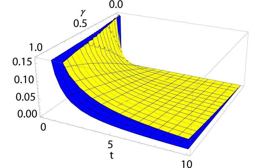
Figure 1: Plot of the response function $\xi_{G}(t)$ versus $\gamma\in(0,1)$ and $t\in(0,10)$ for $\{\alpha=1/2,\beta=\gamma/2,\gamma\}$ (dark grey/blue surface) and $\{\alpha=1/2,\beta=2\gamma/3,\gamma\}$ (light grey/yellow surface).

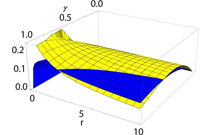
Figure 2: Plot of the spectral distribution $K_{1/2,\gamma/2}^{\gamma}(r)$ (dark grey/blue surface) and $K_{1/2,2\gamma/3}^{\gamma}(r)$ (light grey/yellow surface) for $0<\gamma<1$ and $0\leq r\leq 10$.

Figure 3: Plot of the response function $\xi_{G}(t)$ versus $\alpha\in(0,1)$ and $t\in(0,10)$ for $\{\alpha,\beta=\alpha/2,\gamma=1/2\}$ (dark grey/blue surface) and $\{\alpha,\beta=2\alpha/3,\gamma=1/2\}$ (light grey/yellow surface).

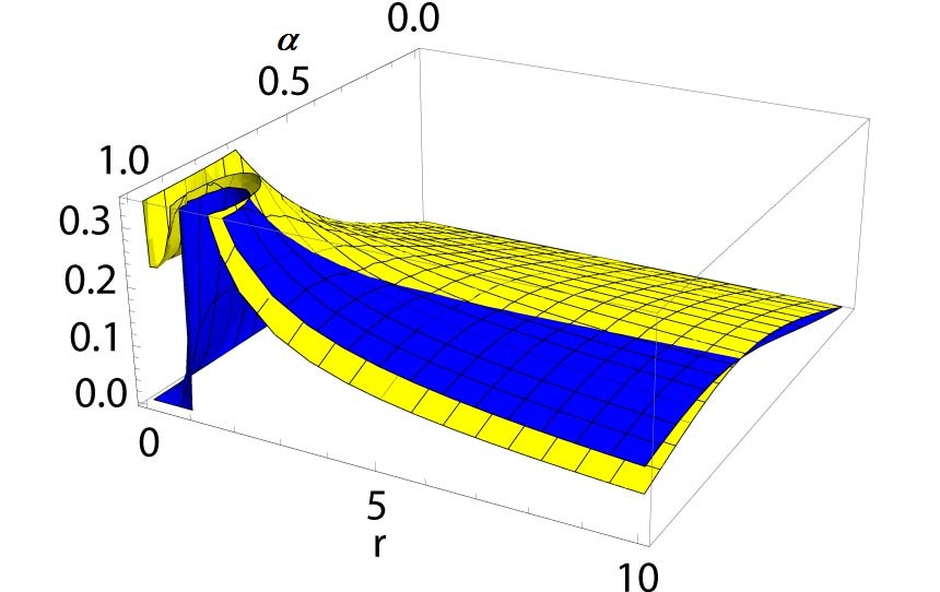
Figure 4: Plot of the spectral distribution $K_{\alpha,\alpha/2}^{1/2}(r)$ (dark grey/blue surface) and $K_{\alpha,2\alpha/3}^{1/2}(r)$ (light grey/yellow surface) for $0<\alpha<1$ and $0\leq r\leq 10$.

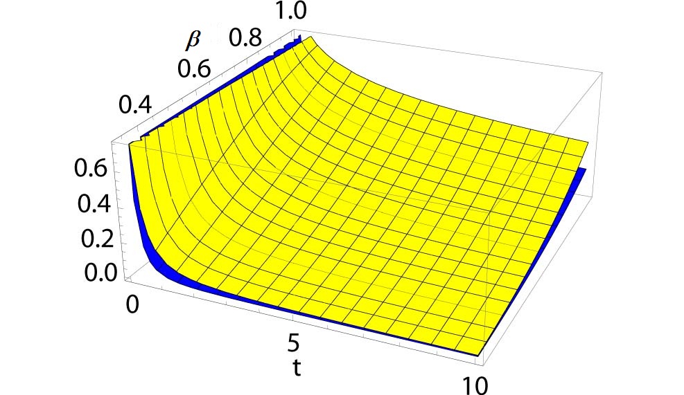
Figure 5: Plot of the response function $\xi_{G}(t)$ versus $\beta\in(1/3,1)$ and $t\in(0,10)$ for $\{\alpha=1/2,\beta,\gamma=1\}$ (dark grey/blue surface) and $\{\alpha=2/3,\beta=2\alpha/3,\gamma=1/2\}$ (light grey/yellow surface).

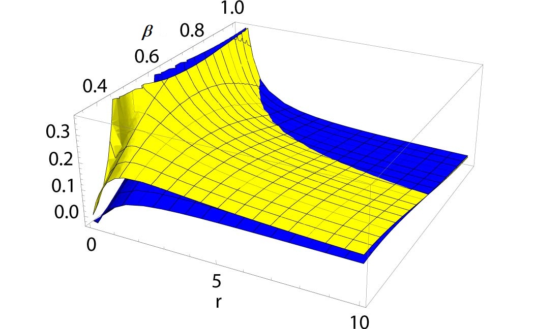
Figure 6: Plot of the spectral distribution $K_{1/2,\beta}^{1}(r)$ (dark grey/blue surface) and $K_{2/3,\beta}^{1/2}(r)$ (light grey/yellow surface) for $1/3<\beta<1$ and $0\leq r\leq 10$. Note that $K_{2/3,\beta}^{1/2}(r)<0$ when the condition $\beta\geq\alpha\gamma$ is not satisfied.

For our plots MATHEMATICA (Wolfram) was used. As far as we know, up to now no official routine exists for the Prabhakar function whereas for the two parameter Mittag-Leffler function a number of authors have provided specific routines and/or numerical methods, see e.g. [5, 6, 17, 38, 39, 47, 50].

4 Conclusions

In this revised paper we have presented a quite general mathematical model for dielectrics that exhibit deviations from the standard relaxation Debye law. This model is based on a time response function expressed in terms of a Mittag-Leffler function with three order-parameters. A restriction on these parameters is required to ensure its complete monotonicity for $t>0$, so that the resulting relaxation process can be seen as a continuous distribution of elementary exponential processes by means of a corresponding (non-negative) spectral distribution function.

Our approach allows one to derive from a unique mathematical framework the classical Cole-Cole, Davidson–Cole and Havriliak–Negami models that are usually adopted in the literature. However, other laws can be derived from our model that could better fit some experimental data.

For some study–cases we have exhibited plots of the response functions (versus $t$) along with their corresponding (non-negative) spectral distributions (versus $r$) keeping fixed two of the three order-parameters $\{\alpha,\beta,\gamma\}$ of our Mittag-Leffler function. We have verified that when the three conditions stated in Eq.(2.21): $0<\alpha\leq 1$, $0<\beta\leq 1$ and $0<\gamma\leq\beta/\alpha$ are not all satisfied the corresponding spectral distributions $K_{\alpha,\beta}^{\gamma}(r)$ turn out to be negative in some ranges of $r$.

As a matter of fact with this revised version we have shown a noteworthy result that improves the conditions outlined by Mainardi in his 2010 book [26] and then by us in our original paper published in Eur. Phys. J.-Special Topics, Vol. 193, pp. 161–171 (2011). With respect to the published versions, we note that condition $0<\gamma\leq 1$ can be relaxed provided that all inequalities in Eq.(2.21) hold true.

We point out that we were inspired by the approach by Hanyga and Seredyńska [9] who have applied the theorem by Gripemberg et al [8] in order to prove the CM of the 3-parameter Prabhakar function in the particular case $\beta=1$.

References

- [1] K. S. Cole and R. H. Cole, Dispersion and absorption in dielectrics. I. Alternating current characteristics, J. Chem. Phys. 9 (1941), 341–351.
- [2] K. S. Cole and R. H. Cole, Dispersion and absorption in dielectrics. II. Direct current characteristics. J. Chem. Phys. 10 (1942), 98–105.
- [3] D. W. Davidson and R. H. Cole, Dielectric relaxation in glycerol, propylene glycol, and -propanol, J. Chem. Phys. 19 (1951), 1484–1490.
- [4] K. Diethelm, The Analysis of Fractional Differential Equations. An Application-Oriented Exposition Using Differential Operators of Caputo Type. (Springer, Berlin, 2010). Springer Lecture Notes in Mathematics No 2004.
- [5] R. Garrappa and M. Popolizio, Evaluation of generalized Mittag–Leffler functions on the real line, Adv. Comput. Math., 39 No. 1 (2013), 205–225.
- [6] R. Gorenflo, J. Loutchko, and Y. Luchko, Computation of the Mittag–Leffler function and its derivative, Fract. Calc. Appl. Anal. 5 No 4 (2002), 491–518. Corrections in Fract. Calc. Appl. Anal. 6 No 1 (2003), 111–112.
- [7] R. Gorenflo and F. Mainardi, Fractional calculus: integral and differential equations of fractional order, in: A. Carpinteri and F. Mainardi (Editors), Fractals and Fractional Calculus in Continuum Mechanics (Springer Verlag, Wien, 1997), 223–276. [E-print: http://arxiv.org/abs/0805.3823].
- [8] G. Gripenberg, S. O. Londen and O. J. Staffans, Volterra Integral and Functional Equations (Cambridge University Press, Cambridge, 1990), pp. 143–147.
- [9] A. Hanyga and M. Seredyńska, On a mathematical framework for the constitutive equations of anisotropic dielectric relaxation. J. Stat. Phys 131 (2008), 269–303.
- [10] H. J. Haubold, A .M. Mathai and R. K. Saxena, Mittag-Leffler functions and their applications, Journal of Applied Mathematics 2-11 ID 298628, 51 pages [doi:10.1155/2011/298628] Hindawi Publ. Co.
- [11] S. Havriliak Jr and S.J. Havriliak, Comparison of the Havriliak-Negami and stretched exponential functions, Polymer 37 No. 18 (1996), 4107–4110.
- [12] S. Havriliak Jr. and S. Negami, A complex plane analysis of -dispersions in some polymer systems, J. Polymer Sci. C 14 (1966), 99–117.
- [13] S. Havriliak and S. Negami, A complex plane representation of dielectric and mechanical relaxation processes in some polymers, Polymer 8 (1967), 161–210.
- [14] H. Hilfer (Editor), Applications of Fractional Calculus in Physics. (World Scientific, Singapore, 2000).
- [15] H. Hilfer, Analytical representations for relaxation functions of glasses. J. Non-Cryst. Solids 305 (2002). 122–126.
- [16] H. Hilfer, function representations for stretched exponential relaxation and non-Debye susceptibilities in glassy systems. Phys. Rev. E 65 (2002), 061510/1–5.
- [17] R. Hilfer and H. Seybold, Computation of the generalized Mittag-Leffler function and its inverse in the complex plane, Integral Transform, Spec. Funct. 17 (2006), 637–652.
- [18] A. K. Jonscher, Dielectric Relaxation in Solids (Chelsea Dielectrics Press, London, 1983).
- [19] A. K. Jonscher, Universal Relaxation Law (Chelsea Dielectrics Press, London, 1996).
- [20] A. Jurlewicz and K. Weron, Infinite divisible waiting-time distributions underlying the empirical relaxation responses, Acta Phyisica Polonica B 31 (2000), 1077–1084.
- [21] A. Jurlewicz and K. Weron, Relaxation of dynamically correlated clusters, J. Non-Cryst. Solids 305 (2002), 112–121.
- [22] A. Jurlewicz, K. Weron and M. Teuerle, Generalized Mittag-Leffler relaxation: Clustering-jump continuous-time random walk approach. Phys. Rev. E 78 (2008), 011103/1–8.
- [23] A. A. Kilbas and M. Saigo, -transforms. Theory and Applications (Chapman and Hall/CRC, Boca Raton, FL, 2004).
- [24] A. A. Kilbas, H. M. Srivastava and J. J. Trujillo, Theory and Applications of Fractional Differential Equations (Elsevier, Amsterdam, 2006).
- [25] V. Kiryakova, Generalized Fractional Calculus and Applications (Longman, Harlow, 1994). [Pitman Research Notes in Mathematics, Vol. 301]
- [26] F. Mainardi, Fractional Calculus and Waves in Linear Viscoelasticity (Imperial College Press, London, 2010).
- [27] F. Mainardi and R. Gorenflo, Time-fractional derivatives in relaxation processes: a tutorial survey, Fractional Calculus and Applied Analysis 10 No 3 (2007), 269–308. [E-print http://arxiv.org/abs/0801.4914].
- [28] A. M. Mathai and H. J. Haubold, Special Functions for Applied Scientists (Springer Science, New York, 2008).
- [29] A. M. Mathai, R. K. Saxena and H. J. Haubold, The -function. Theory and Applications (Springer, New York, 2008).
- [30] K. S. Miller and S. G. Samko, A note on the complete monotonicity of the generalized Mittag-Leffler function. Real Anal. Exchange 23 (1997), 753–755.
- [31] K. S. Miller and S. G. Samko, Completely monotonic functions. Integral Transforms and Special Functions 12 (2001), 389–402.
- [32] R. Nigmatullin and Y. Ryabov, Cole-Davidson dielectric relaxation as a self similar relaxation process, Physics of the Solid State 39 No 1 (1997), 87–90.
- [33] V. V. Novikov, K. W. Wojciechowski, O. A. Komkova and T. Thiel, Anomalous relaxation in dielectrics. Equations with fractional derivatives, Material Science Poland 23 (2005), 977–984.
- [34] I. Podlubny, Fractional Differential Equations (Academic Press, San Diego, 1999).
- [35] H. Pollard, The completely monotonic character of the Mittag-Leffler function . Bull. Amer. Math. Soc. 54 (1948), 1115–1116.
- [36] T. R. Prabhakar, A singular integral equation with a generalized Mittag-Leffler function in the kernel. Yokohama Math. J. 19 (1971), 7–15.
- [37] W. R. Schneider, Completely monotone generalized Mittag-Leffler functions, Expositiones Mathematicae 14 (1996), 3–16.
- [38] H. J. Seybold and R. Hilfer, Numerical results for the generalized Mittag-Leffler function, Fract. Calc. Appl. Anal. 8 (2005), 127–139. (2005)
- [39] H. J. Seybold and R. Hilfer, Numerical algorithm for calculating the generalized Mittag–Leffler function. SIAM J. Numer. Anal. 47 No 1 (2008), 69-–88.
- [40] R. T. Sibatov, V. V. Uchaikin and D. V. Uchaikin, Fractional wave equation for dielectric medium with Havriliak-Negami response in D. Baleanu, J. A. Tenreiro Machado and A.C. J Luo, Fractional Dynamics and Control, Ch. 25, pp. 293–301 (Springer, Berlin 2012).
- [41] A. Stanislavsky, K. Weron and J. Trzmiel, Subordination model of anomalous diffusion leading to the two-power-law relaxation responses, European Physics Letters (EPL 91 (2010), 40003/1–6.
- [42] B. Szabat, K. Weron and P. Hetman, Heavy-tail properties of relaxation time distributions underlying the Havriliak–Negami and the Kohlrausch-Williams-Watts relaxation patterns, J. Non-Cryst. Solids 353 No 47-51 (2007), 4601–4607.
- [43] E. C. Titchmarsh, Introduction to the Theory of Fourier Integrals (Oxford University Press, Oxford, 1937).
- [44] V. V. Uchaikin and R. T. Sibatov, Fractional Kinetics in Solids. Anomalous Charge Transport in Semiconductors, Dielectrics and Nanosystems (World Scientific, Singapore, 2012).
- [45] K. Weron, A. Jurlewicz and M. Magdziarz, Havriliak-Negami response in the framework of the continuous-time random walk,. Acta Phyisica Polonica B 36 (2005), 1855–1868.
- [46] K. Weron and M. Kotulski, On the Cole-Cole relaxation function and related Mittag-Lettter distribution, Physica A 232 (1996), 180–188.
- [47] D. Verotta, Fractional compartmental models and multi-term Mittag–Leffler response functions, J. Pharmacokinet. Pharmacodyn. 37 No 2 (2010), 209–215.
- [48] D. V. Widder, The Laplace Transform (Princeton University Press, Princeton, 1946).
- [49] A. H. Zemanian, Realizability Theory for Continuous Linear Systems (Academic Press, San Diego, 1972).
- [50] C. Zeng and Y-Q Chen, Global Padé approximations of the generalized Mittag-Leffler function and its inverse, E-print arXiv::1310.5592, pp.17.