Abstract

Now that spike trains from many neurons can be recorded simultaneously, there is a need for methods to decode these data to learn about the networks that these neurons are part of. One approach to this problem is to adjust the parameters of a simple model network to make its spike trains resemble the data as much as possible. The connections in the model network can then give us an idea of how the real neurons that generated the data are connected and how they influence each other. In this chapter we describe how to do this for the simplest kind of model: an Ising network. We derive algorithms for finding the best model connection strengths for fitting a given data set, as well as faster approximate algorithms based on mean field theory. We test the performance of these algorithms on data from model networks and experiments.

1 Introduction

Now that we can record the spike trains of large numbers of neurons simultaneously, we have a chance, for the first time in the history of neuroscience, to start to understand how networks of neurons work. But how are we to proceed, once we have such data? In this chapter, we will review some ideas we have been developing. The reader will recognize that we are only describing the very first steps in a long journey. But we hope that they will help point the way toward real progress some time in the not-too-distant future.

What is it we want to learn from multi-spiketrain data? Here we will focus on finding the connectivity in the network under study. We hope that ultimately this can help us understand the dynamics of the network and how it implements computations. For example, in the hippocampus and entorhinal cortex, many interesting kinds of neurons (place cells, grid cells, etc.) have been identified, but we do not know how they interact. If we could find out how they are connected, we might be able to get a much better idea of how they compute the animal’s estimate of its location.

Of course, we will not be able to find the full connectivity unless we can record from all neurons, which is impossible, at least with any current techniques. Several orders of magnitude separate the number of electrodes in a recording array and the number of neuron in the area it covers, so any apparent effect of one neuron on another might actually be mediated by unobserved neurons. Thus, we (and everyone else in the field) are forced into using terms like “effective connections” or “functional connectivity.” In this chapter, for brevity, we will generally just write “connections” or “connectivity”, but we will always mean that they are “effective” or “functional” connections.

Given this fundamental limitation on our project, it is nevertheless worth remarking that while all connections are functional one, some kinds are more functional than others. Modeling approaches that are closer to biophysical reality stand a better chance of recovering something like the real synaptic connectivity than those which are farther away. The approach we describe here is at least a first step, albeit a modest one, in the right direction.

One can take a rather different attitude, proceeding formally and making a purely statistical model: a mathematical object with some parameters that characterize the data. However, even if such a model fits the data well, one has in general no way to assign biological meaning to the parameters. This is not to say that we don’t care about fit quality – we do. It is only to say that fitting, for example, equal-time neuronal firing correlations in the data perfectly with some model is not very satisfying if the parameters of the model cannot be related fairly directly to the connectivity of the network.

To present the models and formal approaches that we study, we have to start with our notation for the data. We work with time-binned spike trains under the assumption that firing rates are low enough that there is (almost) never more than one spike per bin. Time will be measured in units of the bin size. We denote the spike train of neuron $i$ by $S_{i}(t)$, where $S_{i}(t)=+1$ if it fires in bin $t$ and $S_{i}(t)=-1$ if it does not. (One can equivalently use $S_{i}=0$ for no spike, but we won’t do that here.) Thus we can visualize the data as a big array, the “spike matrix” ($N\times T$ if there are $N$ neurons and $T$ time bins), of $+1$s and $-1$s.

This representation of the data lends itself to formulating the problem in terms of a very simple, perhaps the simplest possible model: a McCulloch-Pitts network (McCulloch and Pitts, 1943), or what in physics is called an Ising model. In this chapter we will use several different kinds of Ising models to treat the problem of finding the connections in a network from its spiking history.

2 The Gibbs Equilibrium Model

A possible formal approach to the problem is this (Schneidman et al, 2006): One considers the data as the set of columns on the spike matrix, i.e., all the spike patterns observed, ignoring their temporal order, and asks what distribution they could have been sampled from. Since one is treating all the patterns as coming from the same distribution, one is implicitly assuming stationarity in the data. If one seeks the distribution with the largest entropy, consistent with the sample means $m_{i}=\langle S_{i}\rangle$ and correlations $\langle(S_{i}-m_{i})(S_{j}-m_{j})\rangle$, one finds something with a familiar look (at least if one is a statistical physicist):

$$P[{\bf S}]=\frac{1}{Z}\exp\left[\mbox{$\frac{1}{2}$}\sum_{ij}J_{ij}S_{i}S_{j}+\sum_{i}h_{i}S_{i}\right]$$ (1)

This is the Gibbs equilibrium distribution for the (pairwise) Ising model. Its parameters, $J_{ij}$ and $h_{i}$, are Lagrange multipliers that are used in the constrained maximization. The parameter $J_{ij}$ is the strength with which unit (neuron) $j$ influences unit $i$, and the bias “field” $h_{i}$ controls how likely unit $i$ is to be +1 (“fire”) in the absence of the other units. The expectation values of the $S_{i}$ under the distribution (1), denoted $m_{i}$ (“magnetizations” in the original context of the model), are related to the neuronal firing rates $r_{i}$ (in units of spikes/time bin) through $m_{i}=2r_{i}-1$.

One might like to think of $J_{ij}$ as something like a synaptic strength. However, the $\sf J$ matrix in (1) is necessarily symmetric, $J_{ij}=J_{ji}$. This is true for the couplings in magnets, but it is generally not true for synapses, so we have to be cautious about what $J_{ij}$ means.

A few remarks: In physics, the normalizing denominator $Z$ in (1) is called the partition function, and its log is the negative of the free energy. We are everywhere setting the temperature equal to 1, since changing the temperature just amounts to rescaling the $J_{ij}$s and $h_{i}$s by a constant factor.

Normally in statistical mechanics, one is given a model and its parameters, and the task is to find the moments $\langle S_{i}\rangle$, $\langle S_{i}S_{j}\rangle$, etc., which are the quantities that can be measured in experiments. But here we have an inverse problem: we are given the measured correlation functions and want to find the parameters of the model.

It has been known for some time how to solve this problem, at least in principle. One should adjust the $h_{i}$ and $J_{ij}$ to maximize the probability (1), evaluated on the data. Doing this by gradient ascent gives learning rules

$$\delta h_{i} = \eta(\langle S_{i}\rangle_{\rm data}-\langle S_{i}\rangle_{{\sf J},{\bf h}}),$$ (2)

$$\delta J_{ij} = \eta(\langle S_{i}S_{j}\rangle_{\rm data}-\langle S_{i}S_{j}\rangle_{{\sf J},{\bf h}}).$$ (3)

The averages in the second terms are under the model with the current values of the $J_{ij}$ and $h_{i}$, and $\eta$ is a learning rate, to be chosen small enough to get smooth convergence. To evaluate them exactly, we have to know the probabilities (1), which requires evaluating the partition function $Z$. To do this exactly one has to sum $2^{N}$ terms, which is feasible for systems up to $N\approx 20$. For larger $N$ one has to estimate the averages by Monte Carlo simulations of the model. This fact makes the learning slow, especially when working with data from long recordings. One wants the estimates of the model averages to be as good as the direct data averages in the first terms, so the length of each Monte Carlo run has to be about equal to the number of time bins in the data set. It may take many iterations to reach stationary values of the $J_{ij}$ and $h_{i}$, so this can be a lot of computing. Just what limit this places on the size of systems that can usefully be studied this way depends on patience and the computing resources available, but in our work we found it impractical to try to work with $N>100$.

These learning rules are a special case of what is called Boltzmann learning (Ackley et al, 1985), which also covers systems with “hidden”, i.e., unrecorded units. In this case, the first terms on the right-hand sides of (2) and (3), when evaluated for hidden units, are averages over the model with the visible units clamped to their measured values. This requires even more Monte Carlo runs.

2.1 Mean-field methods

It is possible to avoid long Monte Carlo runs using mean field methods. Two such methods have been proposed. One is based on heuristic mean-field equations first applied to magnetic systems by Weiss more than a century ago. The other is based on improved equations first proposed by Onsager. They were applied to spin glasses by Thouless, Anderson and Palmer (Thouless et al, 1977), so nowadays in statistical mechanics they are called TAP equations.

Both the original mean-field and TAP equations are approximate partial solutions to the forward problem, i.e., calculating the magnetizations $m_{i}$. From them, we will derive corresponding solutions to the inverse problem. These solutions are approximate, but become very good in the limits of weak coupling or, for dense connections, large $N$.

The idea of mean field theory is very simple. The exact $m_{i}$, conditional on a set of $S_{j}$ connected to $i$ by the coupling matrix $J_{ij}$, is the difference of Boltzmann probabilities

$$p(S_{i}=1|\{S_{j}\})-p(S_{i}=-1|\{S_{j}\}) = \frac{{{\rm e}}^{h_{i}+\sum_{j}J_{ij}S_{j}}-{{\rm e}}^{-h_{i}-\sum_{j}J_{ij}S_{j}}}{{{\rm e}}^{h_{i}+\sum_{j}J_{ij}S_{j}}+{{\rm e}}^{-h_{i}-\sum_{j}J_{ij}S_{j}}}$$ (4)

$$= \tanh\left(h_{i}+\sum_{j}J_{ij}S_{j}\right).$$

The approximation consists of replacing the $S_{j}$ inside the tanh by their averages $m_{i}$:

$$m_{i}=\tanh\left(h_{i}+\sum_{j}J_{ij}m_{j}\right).$$ (5)

This is apparently a good approximation when the sum on $j$ has many terms (a loose kind of central-limit argument). This is called the mean field limit.

Onsager argued that the contribution to the neighbor magnetizations $m_{j}$ from the central unit $S_{i}$ itself should not be counted in estimating the field acting on $S_{i}$. This leads to corrected mean-field equations,

$$m_{i}=\tanh\left[h_{i}+\sum_{j}J_{ij}m_{j}-m_{i}\sum_{j}J_{ij}^{2}(1-m_{j}^{2})\right].$$ (6)

TAP showed that these equations, rather than (5), should be used in spin glasses, where the $J_{ij}$ are random, with a zero or very small mean, because then the Onsager correction term is of the same order as the naive mean field. In this sense, these equations are the correct mean field equations for spin glasses. It has become conventional to call them “TAP equations”. We will use the abbreviation “nMF” for the naive mean field equations (5).

Plefka showed that (5) and (6) are the first two in a sequence of better and better approximations that can be derived systematically (Plefka, 1982), but we will only consider these first two here.

It is convenient to write the TAP equations in the form

$$h_{i}=\tanh^{-1}m_{i}-\sum_{j}J_{ij}m_{j}+m_{i}\sum_{j}J_{ij}^{2}(1-m_{j}^{2})$$ (7)

The matrix

$$\chi^{-1}_{ij}=\frac{\partial h_{i}}{\partial m_{j}}=\frac{\delta_{ij}}{1-m_{i}^{2}}-J_{ij}-2J_{ij}^{2}m_{i}m_{j}$$ (8)

is the inverse susceptibility matrix. In equilibrium statistical mechanics there is a theorem that the susceptibility matrix is (up to a factor of the temperature, which we are setting equal to 1) equal to the correlation matrix

$$C_{ij}=\langle(S_{i}-m_{i})(S_{j}-m_{j})\rangle$$ (9)

Thus, if we know the correlation matrix, we simply need to invert it and solve (for $i\neq j$)

$$({\sf C}^{-1})_{ij}=-J_{ij}-2J_{ij}^{2}m_{i}m_{j}$$ (10)

for $J_{ij}$ (Kappen and Rodriguez, 1998; Tanaka, 1998; Roudi et al, 2009). This is the TAP algorithm. There are $n(n-1)/2$ quadratic equations to be solved, but they are decoupled. For the original, “naive” mean field approximation, it is even simpler: The last term on the right hand side of (10) is absent, and we just have $J_{ij}=-({\sf C}^{-1})_{ij}$.

3 Kinetic Ising Models

The Ising model as described so far has no dynamics. It is defined solely by the Gibbs equilibrium distribution (1). Since the system we are trying to understand is a noisy dynamical one, we would like to fit its data – the spike trains – by a stochastic dynamical model. And the Ising model can be given a dynamics in a natural way, as follows (Glauber, 1963). At each time, every neuron has a chance $\propto dt$ of being updated in the infinitesimal interval $[t,t+dt)$ (i.e., neuron updates are independent Poisson processes). For a neuron that is updated, we compute the total “field”

$$H_{i}(t)=h_{i}(t)+\sum_{j}J_{ij}S_{j}(t).$$ (11)

(We can allow the external field $h_{i}$ to depend on time.) We then let $S_{i}$ take its next value $S_{i}(t+\Delta t)$ according to the probability

$$P(S_{i}(t+\Delta t)|\{S_{j}(t)\})=\frac{\exp[S_{i}(t+\Delta t)H_{i}(t)]}{2\cosh H_{i}(t)}=\mbox{$\frac{1}{2}$}[1-S_{i}(t+\Delta t)\tanh H_{i}(t)].$$ (12)

It is then possible to show that if $h_{i}$ is independent of $t$ and the matrix $\sf J$ is symmetric, this model has a stationary distribution given by (1).

Since we would like to identify the $J_{ij}$ with synaptic strengths, which are not symmetric, we relax the symmetry condition. Furthermore, here we will update all the neurons simultaneously instead of randomly asynchronous, because it makes the model easier to apply to time-binned data, such as we are assuming we have here. (We set $\Delta t=1$ from now on.) With either of these changes, the Gibbs equilibrium distribution (1) is no longer a stationary solution of the dynamics, even if the $h_{i}$ are time-independent. In the case that they are and $\sf J$ is symmetric, there is a stationary distribution,

$$P[{\bf S}]=\frac{\prod_{i}[2\cosh(\sum_{j}J_{ij}S_{j}+h_{i})]}{\sum_{\{\sigma\}}\prod_{i}[2\cosh(\sum_{j}J_{ij}\sigma_{j}+h_{i})]}$$ (13)

(Peretto, 1984). When the $h_{i}$ are time-independent and $\sf J$ is not symmetric, a stationary distribution may still exist, but it cannot be written down in closed from. Since such a state is not described by the Gibbs equilibrium distribution (1), we call it a non-equilibrium state, even though it is stationary.

3.1 Stationary case: exact algorithm

For simplicity, we consider first the case where the $h_{i}$ are time-independent and we assume a stationary distribution of the $S_{i}$. If we are given a set of spike trains in the form ${\bf S}=\{S_{i}(t)\}$, $1\leq i\leq N$, we can derive an algorithm for finding the model parameters $J_{ij}$ and $h_{i}$ by performing gradient ascent on the log-likelihood of the data under the model, which is

$$L[{\bf S},{\sf J},{\bf h}]=\sum_{it}[S_{i}(t+1)H_{i}(t)-\log 2\cosh H_{i}(t)],$$ (14)

with $H_{i}(t)$ given by (11). This gives learning rules

$$\delta h_{i} = \eta\left[\langle S_{i}(t+1)\rangle_{t}-\left\langle\tanh H_{i}(t)\right\rangle_{t}\right]$$ (15)

$$\delta J_{ij} = \eta\left[\langle S_{i}(t+1)S_{j}(t)\rangle_{t}-\left\langle\tanh H_{i}(t)S_{j}(t)\right\rangle_{t}\right]$$ (16)

(Roudi and Hertz, 2011a). Equations (15) and (16) have a form analogous to (2) and (3) for the equilibrium case: the right hand sides are differences between averages over the data and averages under the current model. However, here the latter can be evaluated directly and quickly from the data, so this algorithm is generally much faster than the equilibrium one.

It is practical in implementing this algorithm to express the neuronal firing variables in terms of the differences $\delta S_{i}(t)=S_{i}(t)-m_{i}$, with $m_{i}=\langle S_{i}(t)\rangle_{t}$ and to write $H_{i}(t)$ in the form

$$H_{i}(t)=b_{i}+\sum_{j}J_{ij}\delta S_{j}(t)$$ (17)

with

$$b_{i}=h_{i}+\sum_{j}J_{ij}m_{j}.$$ (18)

Then we have

$$\delta b_{i} = \eta\left[m_{i}-\left\langle\tanh H_{i}(t)\right\rangle_{t}\right]$$ (19)

$$\delta J_{ij} = \eta\left\{D_{ij}-\left\langle\left[\tanh H_{i}(t)-m_{i}\right]\delta S_{j}(t)\right\rangle_{t}\right\},$$ (20)

with

$$D_{ij}=\langle\delta S_{i}(t+1)\delta S_{j}(t)\rangle,$$ (21)

the one-step-delayed correlation matrix. The factor in brackets in the time average in (20) can be recognized as the expectation value of $\delta S_{i}(t+1)$, given the measured $S_{j}(t)$, so the second term is the one-time-step delayed correlation matrix for the model, conditional on the data at $t$.

This algorithm is exact, in the sense that for data generated by a kinetic Ising model of this form, it will recover the $J_{ij}$ and $h_{i}$ exactly, after infinite iterations, for infinite data. (By “infinite data” we mean an infinite number of time steps.)

3.2 Stationary case: mean-field methods

Like the equilibrium model, this model allows systematic and rapid mean-field and TAP approximations (Roudi and Hertz, 2011a). To derive the mean-field algorithm, we start by assuming that the $m_{i}$ (of the data) satisfy the mean-field equations (5). Then, on the right-hand side of (16), we write $S_{i}(t)=m_{i}+\delta S_{i}(t)$ and expand the tanh to first order in the $J_{ik}$. First-order terms in $\delta S$ cancel, and we are left with

$$\delta J_{ij}=\langle\delta S_{i}(t+1)\delta S_{j}(t)\rangle-(1-m_{i}^{2})\sum_{k}J_{ik}\langle\delta S_{k}(t)\delta S_{j}(t)\rangle.$$ (22)

If the $J_{ik}$ are the true ones, then we should have $\delta J_{ij}=0$. Thus we obtain a simple matrix equation

$${\sf D}={\sf A}{\sf J}{\sf C}$$ (23)

where

$$C_{ij} = \langle\delta S_{i}(t)\delta S_{j}(t)\rangle$$ (24)

$$A_{ij} = (1-m_{i}^{2})\delta_{ij}$$ (25)

The $J$ matrix can be found simply by matrix inversion and multiplication in terms of first- and second-order statistics of the data:

$${\sf J}={\sf A}^{-1}{\sf D}{\sf C}^{-1}.$$ (26)

Knowing the $J_{ij}$, the inversion task is then completed by solving the MF equations (5) for $h_{i}$:

$$h_{i}=\tanh^{-1}m_{i}-\sum_{j}J_{ij}m_{j}.$$ (27)

Likewise, we can get a TAP approximation by assuming that the $m_{i}$ of the data satisfy the TAP equations (6) and expanding the tanh to third order. After a little algebra, and ignoring some terms which are small for networks with weak, dense connections, we again find the formula (23), but where now

$$A_{ij}=(1-m_{i}^{2})(1-F_{i})\delta_{ij},$$ (28)

with

$$F_{i}=(1-m_{i}^{2})\sum_{k}J_{ik}^{2}(1-m_{k}^{2}).$$ (29)

We cannot solve for the $J_{ik}$ directly in this case, since now $A_{ij}$ depends on them through the $F_{i}$. One way to do it is by iteration, using, say, the mean-field result (26) in (29) to get an initial estimate of $F_{i}$, using this in (28) to get better $J_{ij}$s, and so on. However in the stationary case this iteration can be circumvented by a trick: Since we can write $J_{ik}$ as $J_{ik}^{nMF}/(1-F_{i})$, we can use (29) to obtain

$$F_{i}=\frac{(1-m_{i}^{2})\sum_{k}(J_{ik}^{nMF})^{2}(1-m_{k}^{2})}{(1-F_{i})^{2}},$$ (30)

which is a cubic equation that we can solve for $F_{i}$, given the mean-field $\sf J$. The relevant root is the one that goes to zero as $J_{ij}\to 0$. This root cannot exceed $1/3$, which restricts this method to fairly weak couplings. Still, it is an improvement on the mean-field approximation.

In the same way as for the MF case, once the $J_{ij}$ are found, we can go back to the TAP equations in the form (7) to obtain the $h_{i}$.

3.3 Nonstationary case: exact algorithm

Most of the above carries over to the nonstationary case, where the $h_{i}$ depend on $t$. However, now different time bins are not statistically equivalent, so we require data from (many) runs of the system. Thus, now we will write the spike trains as $S_{i}(t,r)$, where $r$ labels the different runs and $t$ is the time index within a run. The “magnetizations” are now $t$–dependent averages over runs,

$$m_{i}(t)=\langle S_{i}(t,r)\rangle_{r},$$ (31)

and we define $\delta S_{i}(t,r)=S_{i}(t,r)-m_{i}(t)$.

In (14) $S_{i}(t+1)$ and $H_{i}(t)$ acquire a run argument $r$. The learning rules analogous to (19) and (20) are again straightforward to derive by differentiating with respect to $b_{i}(t)$ and $J_{ij}$:

$$\delta b_{i}(t) = \eta\left[m_{i}(t+1)-\left\langle\tanh H_{i}(t,r)\right\rangle_{r}\right]$$ (32)

$$\delta J_{ij} = \eta T\left[D_{ij}-\left\langle\left[\tanh H_{i}(t,r)-m_{i}(t+1)\right]\delta S_{j}(t,r)\right\rangle_{r,t}\right],$$ (33)

where $T$ is the run length and

$$D_{ij}=\langle\delta S_{i}(t+1,r)\delta S_{j}(t,r)\rangle_{r,t}.$$ (34)

Note that it is not the same as the $D_{ij}$ (21) because now the $\delta S_{i}$ are defined relative to the time-dependent run averages $m_{i}(t)$, not the time-independent $m_{i}$.

When we use the word “exact” to describe this algorithm, we mean it in the same sense as for the stationary algorithm, but “infinite data” now means an infinite number of runs to average over in computing the statistics.

3.4 Nonstationary case: mean-field methods

First one needs time-dependent mean-field and TAP equations. These have been derived recently (Roudi and Hertz, 2011b), using a systematic scheme analogous to that employed by Plefka for the equilibrium case. The dynamic TAP equations for the time-dependent magnetizations take the form

$$m_{i}(t+1)=\tanh\left[h_{i}(t)+\sum_{j}J_{ij}m_{j}(t)-m_{i}(t+1)\sum_{j}J_{ij}^{2}(1-m_{j}^{2}(t))\right]$$ (35)

For (naive) mean field, the equations are the same except that the last term inside the brackets is absent.

Now the same procedure that led to (23) gives (Roudi and Hertz, 2011a)

$$D_{ij}=\sum_{k}J_{ik}\langle(1-m_{i}^{2}(t+1))C_{kj}(t)\rangle_{t},$$ (36)

where

$$C_{kj}(t)=\langle\delta S_{k}(t,r)\delta S_{j}(t,r)\rangle_{r}.$$ (37)

If we define a set of matrices ${\sf B}^{(i)}$ by

$$B^{(i)}_{kj}=\langle(1-m_{i}^{2}(t+1))C_{kj}(t)\rangle_{t},$$ (38)

we can again solve for $\sf J$ by simple matrix algebra:

$$J_{ij}=\sum_{k}D_{ik}[({\sf B}^{(i)})^{-1}]_{kj}.$$ (39)

The calculation is a little more time-consuming than the stationary one, because now we have to invert a different matrix ${\sf B}^{(i)}$ for each $i$. Nevertheless, it is still much faster than using the exact algorithm.

For TAP, in the same way as in the stationary calculation, a correction factor $1-F_{i}$ appears. Now $F_{i}$ is time-dependent,

$$F_{i}(t)=(1-m_{i}^{2}(t+1))\sum_{k}J_{ik}^{2}(1-m_{k}^{2}(t)),$$ (40)

and the $(1-F_{i})$-factor enters the time average that defines the matrices ${\sf B}^{(i)}$:

$$B^{(i)}_{kj}=\langle(1-m_{i}^{2}(t+1))(1-F_{i}(t))C_{kj}(t)\rangle_{t},$$ (41)

Now there is no simple equation one can solve for $F_{i}(t)$, as there was in the stationary case, so solving for the $\sf J$-matrix has to be done iteratively.

However, we have found that qualitatively good reconstruction can be done if we make the approximation of factoring the average in (41):

$$\langle(1-m_{i}^{2}(t+1))(1-F_{i}(t))C_{kj}(t)\rangle_{t}\approx(1-F_{i})\langle(1-m_{i}^{2}(t+1))C_{kj}(t)\rangle_{t},$$ (42)

where $F_{i}=\langle F_{i}(t)\rangle_{t}$. Now $F_{i}$ solves a cubic equation, as in the stationary case:

$$F_{i}(1-F_{i}^{2})=\sum_{k}(J_{ik}^{nMF})^{2}\langle(1-m_{i}^{2}(t+1))(1-m_{k}^{2}(t))\rangle_{t},$$ (43)

and, given $F_{i}$, one has $J_{ij}=J_{ij}^{nMF}/(1-F_{i})$, again as in the stationary case.

4 Errors

In a Bayesian way, we can interpret the likelihood $\exp L({\sf J},{\bf b})$ as a probability density for the $J$s and $b$s with a flat prior. This density will peak around the parameters found by the algorithm, and if the data are generated by the kinetic Ising model itself, the peak will lie at their true values in the limit of infinite data. The spread of the probability density around the peak gives a measure of how the parameters obtained from a single data set will vary from one data set to another. Because the log likelihood is proportional to the data set size, it is sufficient, for large $T$ (stationary case) or many runs (nonstationary case) to expand it to second order in the deviations $\delta J_{ij}$ from the values ${\sf J}_{0},{\bf b}_{0}$ at the maximum, so the resulting density is a Gaussian. Suppressing, for simplicity, the dependence on the $b$s and the overall normalization, we find, for the nonstationary case,

$$P({\sf J})\propto\prod_{i}\exp\left(L({\sf J}_{0},{\bf b}_{0})-\mbox{$\frac{1}{2}$}RT\sum_{jk}B_{jk}^{(i)}\delta J_{ij}\delta J_{ik}\right),$$ (44)

where $R$ is the number of runs and the $B_{jk}^{(i)}$ are the matrix elements that occurred above (41) in the mean-field algorithm. Here we can see that $RTB_{jk}^{(i)}$ are the elements of the Fisher information matrix of the distribution of $J$s. The factor of $RT$ means that the fluctuations of the $J$s around their central values go to zero like $1/\sqrt{RT}$ for large data sets. This makes more precise our statement that the exact algorithms described above recover the correct model parameters correctly in the limit of infinite data, if those data are generated by our kinetic Ising model.

To get a little more insight, consider the stationary case, where $B_{jk}^{(i)}=T(1-m_{i}^{2})C_{jk}$. The one can see (1) that $J_{ij}$s with different first (postsynaptic) indices are uncorrelated, and (2) $J_{ij}$s with different second (presynaptic) indices will have strongly correlated errors if they have large projections along eigenvectors of $\sf C$ that have small eigenvalues. Thus, elements of $\sf J$ identified as large by the mean field approximation (26) are exactly the ones for which the estimate is most uncertain. Finally, if correlations in the data are very weak, $\sf C$ is almost diagonal, and

$$\langle\delta J_{ij}\delta J_{ik}\rangle=\frac{\delta_{jk}}{T(1-m_{i}^{2})(1-m_{j}^{2})}.$$ (45)

These considerations show that reconstruction is harder when the data are strongly correlated and when rates are low ($m_{i}$ near -1).

For the mean-field or TAP algorithms, the distribution of $J$s will have a form like (44), but it will not be centered at the true maximum. The mean square errors will be

$$\langle\delta J_{ij}\delta J_{ik}\rangle=\frac{[({\sf B}^{(i)})^{-1}]_{jk}}{RT}+(J_{ij}^{0}-J_{ij}^{\rm true})(J_{ik}^{0}-J_{ik}^{\rm true}).$$ (46)

In cases (such as weak coupling) where the approximations are good, the mean square errors will show the $1/RT$-dependence for small data sets, but for large $RT$ they will level off at a residual value given by the second term in (46).

If the data come from a different model than our kinetic Ising one, we can never obtain its true parameters, even if we use the “exact” algorithms. In this case we say that the model that generated the data was “unrealizable”. The only “realizable” cases are ones where the model used to make the fit is the same as the one used to make the data. When the two models are in some sense close to each other and the $J$s have a meaning in the true model (for example, if we added a term with weak delayed interactions $\sum_{j}K_{ij}S_{j}(t-1)$ to (11)), we can have a situation like that for the approximate algorithms, with errors that first decrease with data set size and then level off at residual values. But in general all we can say is that we have found the best kinetic Ising model, i.e., the kinetic Ising model most likely to have generated the data.

The real “true” model, i.e., nature itself, is far from our kinetic Ising model. Neurons have much more complex dynamics than our model endows them with, and synapses have dynamics of their own that we have ignored entirely in the present formulation. Thus, in applying our methods to neural data, we have to be rather cautious about interpreting the connection strengths $J_{ij}$ that we obtain.

Furthermore, even if we could replace our simple binary units by models with realistic dynamics and include suitable models for the synapses, we could not expect to recover their parameters correctly from an inference procedure like this, because most of the neurons in the true network are not recorded. A typical experiment records spikes of about 100 neurons in a region of cortex of area about 10 ${\rm mm}^{2}$, which contains of the order of a million neurons. Hence, even ignoring the fact that neurons in this region are coupled to many outside it, we have data from only about 0.01% of the local network. It is clearly an audacious project to hope to learn about the network connections and dynamics from such limited data (hence the resort to terms like “functional connectivity” to describe the results).

On the other hand, we have to start somewhere, and the simple description of a neuron as a stochastic element that fires at a rate that is a sigmoidal function of its net input is at least qualitatively consistent with neurophysiology. While we cannot expect to associate all the $J_{ij}$s we find with direct synaptic connections, we would be surprised if the strongest $J_{ij}$s we found were not indicative of synapses between recorded neurons (assuming we had chosen the time bin size for our data sensibly, i.e., around the sum of typical synaptic and membrane time constants). Our findings (Roudi and Hertz, 2011a; Sect 10.6.2 below), as well as results obtained applying this approach to genetic regulatory network networks (Lezon et al, 2006), support this optimism.

5 Regularization

The algorithms above can be given a simple little extra twist that allows us to eliminate the smallest (presumably, least significant) connections in the network in a controlled way. The idea (Tibshirani, 1996; Ravikumar et al, 2010) is to try to minimize a cost function

$$E=-L[{\bf S},{\sf J},{\bf h}]+\lambda\sum_{ij}|J_{ij}|.$$ (47)

In a Bayesian perspective, the addition of this term is the imposition of a prior $\exp(-\lambda\sum|J_{ij}|)$ on the $J_{ij}$. It leads to a new term in the update rules (16), (20) and (33) for $J_{ij}$ proportional to $-\lambda{\rm sgn}J_{ij}$. To see its effect, think of the space of $J$s, with an axis for each pair $ij$. Under learning, the extra term pushes the $J$ vector toward the edges of a hyper-octahedron where many of its components vanish. The regularization parameter $\lambda$ is chosen small, so this is a weak effect for large $J_{ij}$. But it is a big effect for $J_{ij}\sim\lambda$ or smaller, and it tends to drive these $J$s to zero. Thus this modification of the learning performs a kind of automatic pruning of the network, the degree of which we can control by adjusting $\lambda$.

A possibility for another kind of regularization arises in using the nonstationary algorithms described above. The source of the time dependence of the driving fields $h_{i}(t)$ or $b_{i}(t)$ is the time dependence of the measured $m_{i}(t)$, i.e., of the firing rates. For realistic amounts of data (perhaps 100 repetitions of the stimulus in an experiment), one cannot expect to estimate a rate within a time bin to better than 10% accuracy. The apparent rates will fluctuate this much from one time bin to the next, and the inferred $h_{i}(t)$ will inherit these fluctuations. If we believe that the true rates vary more smoothly than this, we can add a further term to the cost function,

$$E_{smooth}=\mbox{$\frac{1}{2}$}\kappa\sum_{it}[h_{i}(t)-h_{i}(t+1)]^{2}.$$ (48)

The resulting extra term in $\delta h_{i}(t)$ is proportional to $\kappa[h_{i}(t-1)-2h_{i}(t)+h(t+1)]$. This smoothes $h_{i}$ by averaging $h_{i}(t)$ a little with $h_{i}(t\pm 1)$.

6 Testing the Models

We have tested these models on three kinds of data:

(1) Data generated by the models themselves, where we can measure directly how well they recover the (known) network parameters.

(2) Data generated by a semi-realistic computational model of a cortical network. This model is much more complex than the kinetic Ising model we try to fit its data with, but we still know the true connectivity of the network.

(3) Data recorded from a real biological network, in this case of salamander retinal ganglion cells.

6.1 Testing the models on themselves

Testing the algorithms described above on how well they reconstruct the couplings of a kinetic Ising model has two purposes: (1) For the exact algorithms, to verify that they work according to the theoretical picture set out above, in particular, checking that the mean square errors fall off like $1/T$ (stationary case) or $(RT)^{-1}$ (nonstationary case). (2) For the approximate algorithms, evaluating the average residual error in (46) and studying how it depends on the strength of the couplings in the model. We summarize the findings (Roudi and Hertz, 2011a) here.

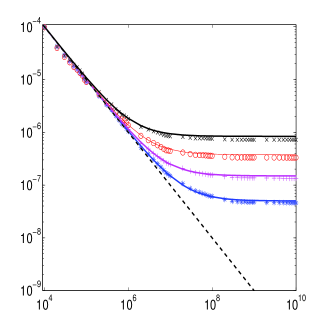
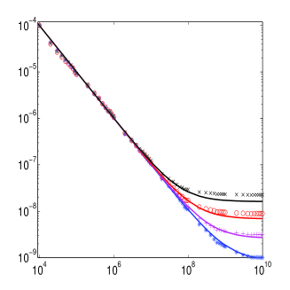
Figure 1: Mean square errors for nMF (a) and TAP (b) approximations, stationary kinetic Ising model, as a function of the number of time steps $T$ in the training data for noise levels g = 0.1 (*), 0.12 (+), 0.14 (circles), and 0.16 (x). The solid lines are the theoretical predictions from equations (52) (nMF) and (53) with finite-size corrections (TAP), and the symbols are the errors measured for the $J$s obtained from the algorithms. The dashed line is the rms error $1/T$ for the exact algorithm. (adapted from Roudi and Hertz, 2011)

Fig. 1 shows mean square errors in the $J$s for a model in which the $J_{ij}$ are chosen independently from a Gaussian distribution of mean zero and standard deviation $g/\sqrt{N}$, where $N$ is the number of neurons in the network. Here we have taken $N=20$ and all $h_{i}=0$. The nMF and TAP errors follow the exact-algorithm result $1/T$ for small $T$ and then flatten out at minimum values (higher for nMF that TAP).

The asymptotic nMF and TAP errors are systematic: For infinite data, nMF systematically underestimates the magnitude of the $J_{ij}$ and TAP overestimates them (though less so). In fact, the factor $1-F_{i}$ relating the TAP and nMF $J_{ij}$s is the lowest-order correction of the nMF underestimation. We can see this simply, for zero field, by expanding the tanh in (16) or (20) at $\delta J_{ij}=0$ to third order in the $J$s (instead of just to linear order as we did in (22)). We get

$$D_{ij}=\sum_{k}J_{ik}C_{kj}-\mbox{$\frac{1}{3}$}\sum_{klm}J_{ik}J_{il}J_{im}\langle S_{k}S_{l}S_{m}S_{j}\rangle+\cdots.$$ (49)

(All correlations here are equal-time.) In the sum over $k$, $l$ and $m$, terms with $k=l$, $l=m$ and $m=k$ dominate. Multiplying on the right by the inverse of ${\sf C}$ and using the nMF result (26), we find

$$J_{ij}^{\rm nMF}=J_{ij}-\left(\sum_{k}J_{ik}^{2}\right)J_{ij}$$ (50)

(plus corrections of relative order $1/N$). Now we can use the fact that for our SK-like model, the quantity $\sum_{k}J_{ik}^{2}=g^{2}$, again ignoring corrections of higher order in $1/N$, so we obtain

$$J_{ij}=\frac{J_{ij}^{\rm nMF}}{1-g^{2}}.$$ (51)

The denominator can be recognized as the TAP correction factor $1-F_{i}$ when the $h_{i}=0$. This implies an asymptotic mean square error

$$\epsilon_{\rm nMF}=\langle(J_{ij}-J_{ij}^{\rm nMF})^{2}\rangle=\frac{g^{6}}{N}.$$ (52)

The solid curves in Fig 1a are $1/T+\epsilon_{\rm nMF}$, evidently a quite good fit for the values of $g$ from 0.1 to 0.16 for which they are plotted. The black dots in Fig 2 show the nMF $J$s plotted against the true ones. When the size of the data set is increased from $10^{4}$ to $10^{6}$, the scatter is reduced and the systematic underestimation becomes clear. In the limit of infinite data, we expect the scatter to disappear, leaving a clean linear behavior near $J_{ij}=0$ with a slope $1-g^{2}$.

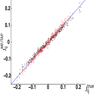
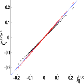
Figure 2: $J$’s obtained by nMF (circles) and TAP (crosses) algorithms, plotted against the true $J$s for a network of 20 neurons with $g=0.35$. (a) $T=10^{4}$; (b) $T=10^{6}$.

The TAP errors shown in Fig 1b are much smaller that the nMF ones, because they include the lowest-order correction (51). We can find the leading error in the TAP approximation by expanding the tanh in (16) to fifth order. A little algebra like that leading to (52) leads to an asymptotic error estimate

$$\epsilon_{TAP}=\frac{4g^{10}}{N}.$$ (53)

Furthermore, one can show that TAP systematically overestimates the magnitudes of the $J$s, in the same way that nMF underestimated them. For a large network, we expect this to describe the asymptotic TAP error. However, there are finite-size corrections, of order $g^{6}/N^{3}$. These would be negligible for $N\gg 1/g^{2}$, but they are not for the small network ($N=20$) at the values of $g$ studied here. However, taking both (53) and the finite-size corrections into account, we are able to account for the measured errors (Fig. 1b).

In Fig 2 one can see that the TAP $J$s (square markers) lie much closer to the true ones than the nMF $J$s (*) do, but a careful look at Fig 2b reveals the systematic overestimation.

Finally, we give an example of nonstationary inference. We generated $R=100$ runs, each of length $T=10^{5}$ steps for a model with $h_{i}=0.5\cos(2\pi t/100)$. The couplings are small enough ($g=0.05$) that nMF is quite accurate, as Fig 3a shows. Furthermore, the fields are also quite well recovered (dots, Fig 3c) by solving (35) (without the TAP term) for $h_{i}(t)$.

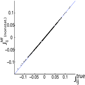
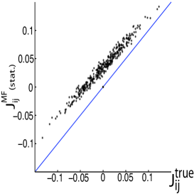
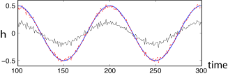
Figure 3: Nonstationary inference: 20 neurons, $g=0.05$, driven by a sinusoidal field with period 100 steps. (a) The couplings inferred using the nonstationary nMF algorithm are almost equal to the true ones. (b) Couplings inferred using the stationary algorithm are systematically overestimated. (c) The nonstationary algorithm recovers the driving field (solid curve) correctly (dots), while the amplitude of the field predicted from the mean field equations using the couplings found by the stationary algorithm (crosses) is too small. (adapted from Roudi and Hertz, 2011)

The $J$s obtained if one does the calculation assuming stationarity are systematically too large (Fig 3b). This is because of the apparent correlations induced in the data by the common external field. In calculating correlations we should actually compute $\langle\delta S_{i}(t)\delta S_{j}(t^{\prime})\rangle_{r}$ using $\delta S_{i}(t)=S_{i}(t)-m_{i}(t)$, with time-dependent $m_{i}(t)$. However, if we assume stationarity and use $\delta S_{i}(t)=S_{i}(t)-\langle m_{i}(t)\rangle_{t}$, instead, we will overestimate the correlations. (This is sometimes called “stimulus-induced correlations”.) These spurious correlations (all positive, in this case) then lead to a spurious increase in the inferred $J_{ij}$s. One can use these spurious $J$s in (35) (again, here with the TAP term absent) to infer $h_{i}(t)$, but because the $J$s are too big, the resulting $h_{i}(t)$ do not have a modulation amplitude as large as they should (Fig 3c, crosses).

6.2 Application To Data From Model Cortical Network

For a first nontrivial test of the approach, we try it on data generated by a realistic model cortical network (Hertz, 2010). This is a network of 1000 spiking neurons, 80% excitatory and 20% inhibitory, with Hodgkin-Huxley-like intrinsic dynamics. They are driven by an additional external population of 800 Poisson neurons firing tonically at 10 Hz. All neurons, both internal and external, are connected by conductance-based synapses in a random fashion, with a connection probability of 10% (except that the external neurons are not connected to each other). The strengths of these synaptic conductances were chosen so that the network was in a high-conductance balanced state (Amit and Brunel, 1997; van Vreeswijk and Sompolinsky, 1998) with average conductances in the range measured experimentally (Destexhe et al, 2003).

The magnitudes of the synaptic conductances did not vary within a class (excitatory-to-excitatory, excitatory-to-inhibitory, etc.), except for the fact that 90% of them were zero because of the random dilution, though they did vary somewhat in their temporal characteristics. For such a system, a natural and important question to ask is how well we can identify the connections that are actually present.

We choose for analysis the spike trains of the inhibitory neurons with rates over 10 Hz. There were 95 of them. Their mean rate was 32 Hz, with a maximum of 83 Hz. Higher firing rates give better statistics, and the inhibitory synapses are the strongest ones in this model, so this choice makes the task of fitting the model and identifying the connections present easier than it might otherwise be. However, it is useful to test the method on an easier problem before trying to solve a more difficult one. The data were put into the form to be used by the algorithms by binning the spikes with 10-ms bins.

To study how much data is necessary for the fit, we did the analysis using the exact stationary algorithm for data sets of size $T$ from 1000 up to 64000 time bins. For each such $T$, we calculated the log likelihood of the data. For comparison, we also calculated these numbers for independent-neuron models based on the same partial data sets. The results were adjusted with Akaike corrections equal to the number of parameters in the models (Akaike, 1974).

Fig 4 shows the log likelihoods (per time step, per neuron), with and without Akaike corrections. They appear to converge to a value of $-0.306\pm 0.001$, and evidently there is little point in using more than around 50000 time steps of data. Also shown are the log likelihoods for an independent-neuron model (all $J_{ij}=0$). For these, the Akaike correction is so small that the corrected and uncorrected curves would fall almost on top of each other, so only the adjusted values are actually plotted. The curve is nearly flat at at value of about -0.53. It is evident that the model with $J$s is much better than the one without them.

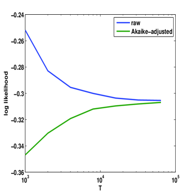
Figure 4: Cortical model data (tonic firing): Log likelihoods as a function of data set size $T$ for fits with kinetic Ising and independent-neuron models. Dashed line: log likelihood. Solid line: Akaike-adjusted log likelihood. Dotted line: independent-neuron model ($J_{ij}=0$). Despite its greater number of parameters, the model with couplings is clearly better, and the difference is evident for all the data set lengths in the range shown.

The Akaike-adjusted log likelihood is a suitable statistic for comparing model quality, but one does not have an clear idea of what a value of -0.306 means for the quality of the network reconstruction, in particular for the problem of identifying the connections present in this diluted network. To do this, we use another statistic, defined as follows.

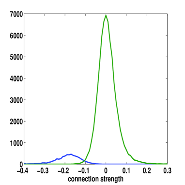
Figure 5: Distributions of connection strengths found for cortical model network data for inhibitory connections present in the network (solid line) and connections not present in the network (dashed line). Averages of results of performing nMF inference on 30 sets of 50 neurons chosen randomly from the 95 inhibitory neurons with rates $>10$ Hz.

Consider the values of $J_{ij}$ that the algorithm finds for the connections that are actually present in the network. These estimates will have some spread around their mean value, because of the limited data and the mismatch between the kinetic Ising model and the real network. For the same reason, the values assigned to the $J_{ij}$s for which the connections $\{ij\}$ are not present, which should be zero, will also be spread around their (small) mean value (Fig 5). If the spreads of these two distribution are small compared to the difference between their means, we can easily identify the true connections, even if we do not know which ones they are a priori. A measure of the difficulty of the task which we can compute (knowing the true connectivity) is the noise/signal ratio

$$d\equiv\frac{\sigma(J_{\rm true}\neq 0)+\sigma(J_{\rm true}=0)}{|\langle J\rangle_{J_{\rm true}\neq 0}-\langle J\rangle_{J_{\rm true}=0}|},$$ (54)

where the standard deviations and means are over the $J$s found by the algorithm. Fig 6 shows $d$ as a function of data set size $T$, calculated for the $J$s obtained by both the exact algorithm and the nMF and TAP approximate formulae. The TAP and nMF results are too close to each other to distinguish, so only the latter is plotted. The plot in Fig 5 was made using TAP results for $T=200000$ and shows the kind of errors one makes for $d\approx 0.47$: The false positive rate is 5.6% and the false negative rate is 7.2%. For $d\approx 0.3$, which one achieves with the exact algorithm, there are almost never any errors.

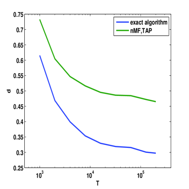
Figure 6: Fitting cortical network data: Noise/signal ratio $d$, as function of data set length $T$ for nMF (dashed) and exact (solid) learning algorithms.

Note, furthermore, that this reconstruction was achieved for a strongly undersampled network – There were 1000 neurons in the network but the reconstructions were done using only 50 of them at a time. This lends some support to our hope that reconstruction, at least for strong synapses, might be possible even though we cannot record from all the neurons in the network.

In this example, we used the stationary versions of the algorithms because the rate of the external driving population was constant. We have also studied a case where the external rate varies in time, performing the corresponding nonstationary analysis, which gives similar results. Results will be published elsewhere.

6.3 Application To Data From Salamander Retina

We have also analyzed a data set provided by Michael Berry of recordings from 40 ganglion cells in a salamander retina. The retina was stimulated 120 times by a 26.5-s movie clip (a total recording time of 3180 s). A nonstationary treatment is natural, in view of the time-dependent stimulus. We expect a significant contribution to the connections identified in a stationary analysis from stimulus-induced correlations, as in Fig 3b.

Such data have been analyzed in the past using the Gibbs equilibrium analysis described in Section 2 (Schneidman et al 2006), which assumes stationarity. It is interesting to see whether the $J_{ij}$s obtained that way are related to those obtained using a stationary kinetic Ising model. They are not expected to be the exactly the same, since the Gibbs $J$s are determined solely by the equal-time correlations and the kinetic Ising ones depend on the one-time-step delayed correlations. Nevertheless, we can hope that if we have chosen the time bin size sensibly, the connections identified by the two methods will be similar.

To find out, we fit both the Gibbs model and the stationary version of our kinetic Ising model to these data. Fig. 7a shows a scatter plot of the resulting two sets of $J_{ij}$s. While they are not so similar as to be concentrated along a straight line in the plot, they do tend to have the same sign (most of the points are in the first or third quadrants).

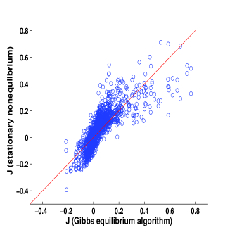
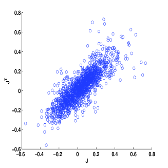
Figure 7: Fig 7. Salamander retina data: (a) Couplings found from the stationary kinetic Ising model algorithm plotted against those obtained from the Gibbs equilibrium algorithm. (b) Testing for the degree of symmetry in couplings: elements of the coupling matrix $\sf J$ plotted against those of its transpose.

The kinetic Ising model allows for an asymmetric $\sf J$ matrix, while symmetry is enforced in the Gibbs model. To see how asymmetric the kinetic Ising $\sf J$ matrix is here, we made a scatter plot of the elements of $\sf J$ against those of its transpose (Fig 7b). Evidently, the magnitudes of $J_{ij}$ and $J_{ji}$ can be different, but they do not differ wildly, and they almost always agree in sign. This is consistent with the fact that they agree qualitatively with the fully symmetric $J$s found for the Gibbs model and with our expectation that they may be the result, to a strong degree, of stimulus-induced correlations, which are symmetric by definition.

To find out to what degree, we then performed a nonstationary analysis, with time-dependent $b_{i}(t)$ in our kinetic Ising model. In addition, we made a fit for a model (also nonstationary) with independent neurons, in which all time dependence of firing rates is explained in terms of the time-dependent $b$s.

We compared these three models on the basis of the log likelihoods of the data under them, with Akaike corrections for the different numbers of model parameters. We found that the stationary model (Akaike-adjusted log likelihood per neuron per time bin $-0.128$ bits) was significantly worse than the nonstationary ones ($-0.0927$ bits for the independent model and $-0.0906$ bits for the full model). The difference between the fits given by the nonstationary models with and without $J_{ij}$s is quite small (0.0021 bits, only 2.4% of the total log likelihood). A full description of this analysis will be published elsewhere.

We conclude that essentially all the connections found for the stationary and Gibbs models come from stimulus-induced correlations. Once we include time-dependent $b$s in the model, adding $J$s gives almost no improvement in the fit. Although it is disappointing not to be able to identify any important intrinsic connections in this network, the result illustrates how the nonstationary analysis can uncover features of the system that stationary models (including the Gibbs model) can not.

7 Further Developments

In all the above, we restricted the treatment to the simplest kind of kinetic Ising model, for pedagogical purposes. It is not hard to extend the model in various ways to bring it closer to neurobiological reality. The most obvious way is to modify the memory-less dynamics (11-12) by letting the firing probability at $t+1$ depend on spikes earlier than $t$:

$$H_{i}(t)=h_{i}(t)+\sum_{j,s=1}^{\tau}J_{ij}(s)S_{j}(t-s+1).$$ (55)

Thus, each connection in the model is characterized by a temporal kernel $J_{ij}(s)$. It describes synaptic and membrane potential dynamics. It is straightforward to derive exact and mean-field learning algorithms for such a model.

Models of this kind, called generalized linear models (GLMs), have been studied in recent years (Truccolo et al, 2004; Okatan et al, 2006). They were used (Pillow et al, 2008) in an extensive study of the signaling by a population of 27 monkey retinal ganglion cells. They have also been used (Rebesco et al, 2010) to track changes in connection strengths in a network in which synaptic plasticity was induced by microstimulation. Thus, the feasibility and utility of such solutions of the inverse problem for real neural networks have been demonstrated. The simple cases described in this chapter can be thought of as “poor man’s” GLMs. Since they have fewer parameters, they may be particularly useful models when data are limited. It may also be useful to extend the mean-field methods discussed here to GLMs.

Another couple of directions in which further development of these models would be useful are the following:

(1) As mentioned above, one never records from all the neurons in a network. A systematic approach to the inference problem in the presence of “hidden units” is needed. This problem could usefully be explored first for the simplest model (11-12) in a realizable case, to gain some knowledge about how to model the hidden part of the population.

(2) Even the model with temporal synaptic kernels assumes “current-based” synapses, i.e., that a presynaptic spike causes a particular current to flow in or out of the postsynaptic neuron, independent of the state of that neuron. Actually, what the presynaptic spike causes is the stochastic opening and closing of a channel, selective for particular ions, in the postsynaptic membrane. The synaptic current (or, more precisely, its average over many presynaptic transmitter release events) is then the product of the conductance of the channel if it were open, the time-dependent probability that it is open, conditional on the presynaptic spike, and the difference between the instantaneous postsynaptic membrane potential and the reversal potential for that channel. The difference between such “conductance based” synapses and current-based ones may be quantitatively small for excitatory synapses, since their reversal potentials are far above the firing threshold, but they are not for inhibitory ones, whose reversal potentials are not much lower than typical subthreshold membrane potentials. It would be desirable and interesting to extend the kind of modeling here to include a little of this potentially relevant biophysics, starting perhaps with the limiting case of “shunting inhibition”.

(3) Finally, we mention a new mean-field inversion algorithm (Mézard and Sakallariou, 2011; Sakallariou et al, 2011) which reconstructs kinetic Ising models exactly when the $\sf J$ matrix is completely asymmetric. It would be interesting to see how well it works on data from more realistic models or experiments.

Ackley D, Hinton GE, Sejnowski TJ (1985) A learning algorithm for Boltzmann machines. Cognitive Science 9:147-169.
Akaike H (1974) A new look at the statistical model identification. IEEE Trans Aut Control 19:716 723.
Amit DJ, Brunel N (1997) Model of global spontaneous activity and local structured activity during delay periods in the cerebral cortex. Cerebral Cortex 7:237-252.
Destexhe A, Rudolph M, Paré D (2003) The high-conductances state of cortical neurons in vivo. Nature Reviews Neurosci 4:739-751.
Glauber RJ (1963) Time-dependent statistics of the Ising model. J Math Phys 4:294-307.
Hertz, J (2010) Cross-correlations in high-conductance states of a model cortical network. Neural Comp 22:427-447.
Kappen HJ, Rodriguez FB (1998) Efficient learning in Boltzmann machines using linear response theory. Neural Comp 10:1137-1156.
Lezon TR, Banavar JR, Cieplak M, Maritan A (2006) Using the principle of entropy maximization to infer genetic interaction networks from gene expression patterns. Proc Nat Acad Sci USA 103:19033 19038.
McCulloch WS, Pitts W (1943) A logical calculus of ideas immanent in nervous activity. Bull Math Biophys 5:115-133.
Mézard M, Sakallariou J (2011) Exact mean field inference in asymmetric kinetic Ising systems. arXiv:1103.3433.
Okatan M, Wilson MA, Brown EN (2005) Analyzing functional connectivity using a network likelihood model of ensemble neural spiking activity. Neural Comp 17:1927-1961.
Peretto P (1984) Collective properties of neural networks: a statistical physics approach. Biol Cybern 50:51-62.
Pillow JW, Shlens J, Paninski L, Sher A, Litke AM, Chichilnisky EJ, Simoncelli EP (2008) Spatio-temporal correlations and visual signalling in a complete neuronal population. Nature 454:995-999.
Plefka T (1982) Convergence conditions of the TAP equation for the infinite-ranged Ising spin glass model. J Phys A 15:1971-1978.
Ravikumar P, Wainwright M, Lafferty JD (2010). High-dimensional Ising model selection using $\ell_{1}$-regularised logistic regression. Ann Stat 38:1287-1319.
Rebesco JM, Stevenson IH, Körding KP, Solla SA (2010) Rewiring neural interactions by micro-stimulation. Frontiers System Neurosci 4:39.
Roudi Y, Hertz J (2011a) Mean-field theory for nonequilibrium network reconstruction. Phys Rev Lett 106:048702.
Roudi Y, Hertz J (2011b) Dynamical TAP equations for non-equilibrium spin glasses. J Stat Mech P03031.
Roudi Y, Tyrcha J, Hertz J (2009) The Ising model for neural data: model quality and approximate methods for extracting functional connectivity. Phys Rev E 79:051915.
Sakellariou J, Roudi Y, Mézard M, Hertz J (2011) Effect of coupling asymmetry on mean-field solutions of direct and inverse Sherrington-Kirkpatrick model. arXiv:1106.0452.
Schneidman E, Berry MJ II, Segev R, Bialek W (2006) Weak pairwise correlations imply strongly correlated network states in a neural population. Nature 440:1007-1012.
Tanaka T (1998) Mean-field theory of Boltzmann learning. Phys Rev E 58:2302-2310.
Thouless DJ, Anderson PW, Palmer RG (1977) Solution of ‘solvable model of a spin glass’. Phil Mag 35:593-601.
Tibshirani R (1996) Regression shrinkage and selection via the lasso. J Roy Stat Soc B 58:267-288.
Truccolo W, Eden UT, Fellows MR, Donoghue JP, Brown EN (2004) A point process framework for relating neural spiking activity to spiking history, neural ensemble, and extrinsic covariate effects. J Neurophysiol 93:1074-1089.
Van Vreeswijk C, Sompolinsky H (1998) Chaotic balanced state in a model of cortical circuits. Neural Comp 10:1321-1371.