The penetrable square-well model: extensive versus non-extensive phases

Abstract

The phase diagram of the penetrable square-well fluid is investigated through Monte Carlo simulations of various nature. This model was proposed as the simplest possibility of combining bounded repulsions at short scale and short-range attractions. We prove that the model is thermodynamically stable for sufficiently low values of the penetrability parameter, and in this case the system behaves similarly to the square-well model. For larger penetration, there exists an intermediate region where the system is metastable, with well defined fluid-fluid and fluid-solid transitions, at finite size, but eventually becomes unstable in the thermodynamic limit. We characterize the unstable non-extensive phase appearing at high penetrability, where the system collapses into an isolated blob of a few clusters of many ovelapping particles each.

I Introduction

Unlike simple fluids, complex fluids are typically characterized by a significant reduction in the number of degrees of freedom, in view of the hierarchy of different length and energy scales involved. As a result, coarse-grained potentials accounting for effective interactions between a pair of the complex fluid units adopt analytical forms that are often quite different from those considered paradigmatic for simple fluids Likos01 .

An important example of this class of potentials is given by those bounded at small separations, thus indicating the possibility of a partial (or even total) interpenetration. This possibility, completely unphysical in the framework of simple fluids, becomes on the contrary very realistic in the context of complex fluids. While the true two-body interactions always include a hard-core part, accounting for the fact that energies close to contact raise several orders of magnitude, effective interactions obtained upon averaging microscopical degrees of freedom may or may not present this feature, depending on the considered particular system.

Interesting examples with no hard-core part are given by polymer solutions, where effective polymer-polymer interactions can be argued to be of the Gaussian form Stillinger76 ; Bolhuis01 ; McCarty10 , and star polymers and dendrimers where the so-called penetrable sphere (PS) model is frequently employed Marquest89 ; Likos98 ; Mladek08 .

In spite of their markedly different phase behaviors Mladek08 , both these effective interactions have the common attributes of being bounded at zero separation and lacking an attractive part. The latter feature, however, appears to be particularly limiting in view of the several sources of attractive interactions typical of polymer solution, such as, for instance, depletion forces Bolhuis01 , that are typically accounted through simple attractive square-well (SW) tails.

A tentative of combining both the penetrability at small separation and the attraction at slighty larger scale, led to the introduction of the penetrable square-well (PSW) potential Santos08 ; Fantoni09 ; Fantoni10a ; Fantoni10b ; Mukamel2009 . This can be obtained either by starting from the PS model and adding an attractive well, or by starting from the SW model and reducing the infinite repulsive energy to a finite one. In this way, the model is characterized by two length scales (the soft core and the width of the well) and by two energy scales, the height $\epsilon_{r}$ of the repulsive barrier and the depth $\epsilon_{a}$ of the attractive well.

The ratio $\epsilon_{a}/\epsilon_{r}$, hereafter simply referred to as “penetrability”, is a measure of the accessibility of the repulsive barrier and, as we shall see, plays a very important role in the equilibrium properties of the fluid. When $\epsilon_{a}/\epsilon_{r}=0$, the PSW model reduces to the PS model (if $k_{B}T/\epsilon_{r}=\text{finite}$, where $T$ is the temperature) or to the SW model (if $k_{B}T/\epsilon_{a}=\text{finite}$). In the latter case, the model exhibits a fluid-fluid phase transition for any width of the attractive square well Vega92 ; deMiguel97 ; delRio02 ; Liu05 ; Giacometti09 , this transition becoming metastable against the formation of the solid for a sufficiently narrow well Liu05 . As penetrability $\epsilon_{a}/\epsilon_{r}$ increases, different particles tend to interpenetrate more and more because this becomes energetically favorable (the precise degree depending on the $\epsilon_{a}/\epsilon_{r}$ ratio). As a result, the total energy may grow boundlessly to negative values and the system can no longer be thermodynamically stable. The next question to be addressed is whether this instability occurs for any infinitesimally small value $\epsilon_{a}/\epsilon_{r}>0$ or, conversely, whether there exists a particular value where the transition from stable to unstable regime occurs.

As early as the late sixties, the concept of a well-behaving thermodynamic limit was translated into a simple rule, known as Ruelle’s criterion Fisher66 ; Ruelle69 , for the sufficient condition for a system to be stable. In a previous paper Santos08 , we have discussed the validity of Ruelle’s criterion for the one-dimensional PSW case and found that, indeed, there is a well-defined value of penetrability $\epsilon_{a}/\epsilon_{r}$, that depends upon the range of the attractive tail, below which the system is definitely stable. Within this region, the phase behavior of the fluid is very similar to that of the SW fluid counterpart. More recently Fantoni11 , we have tackled the same issue in the three-dimensional fluid. Here we build upon this work by presenting a detailed Monte Carlo study of the phase diagram for different values of penetrability and well width. In this case the PSW fluid is proven to satisfy Ruelle’s criterion below a well-defined value of penetrability that is essentially related to the number of interacting particles for a specific range of attractive interaction. For higher values of penetrability, we find an intermediate region where, although the system is thermodynamically unstable (non-extensive) in the limit $N\to\infty$, it displays a “normal” behavior, with both fluid-fluid and fluid-solid transitions, for finite number of particles $N$. The actual limit of this intermediate region depends critically upon the considered temperatures, densities, and size of the system. Here the phase diagram is similar to that of the SW counterpart, although the details of the critical lines and point location depend upon the actual penetrability value. For even higher penetrability, the system becomes unstable at any studied value of $N$ and the fluid evolves into clusters of overlapping particles arranged into an ordered phase at high concentration, with a phenomenology reminiscent of that displayed by the PS model, but with non-extensive properties.

The remaining of the paper is organized as follows. In Section II we define the PSW model and in Section III we set the conditions for Ruelle’s criterion to be valid. The behavior of the system outside those conditions is studied in Section IV, where we also determine the fluid-fluid coexistence curves for the PSW model just below the threshold line found before; in Section V we determine the instability line, in the temperature-density plane, separating the metastable normal phase from the unstable blob phase. Section VI is devoted to the fluid-solid transition and in Section VII we draw some conclusive remarks and perspectives.

II The Penetrable Square-Well model

The PSW model is defined by the following pair potential

$$\phi(r)=\left\{\begin{array}[]{cl}\epsilon_{r}~{},&r\leq\sigma~{},\\ -\epsilon_{a}~{},&\sigma<r\leq\sigma+\Delta~{},\\ 0~{},&r>\sigma+\Delta~{},\end{array}\right.$$ (4)

where $\epsilon_{r}$ and $\epsilon_{a}$ are two positive constants accounting for the repulsive and attractive parts of the potential, respectively, $\Delta$ is the width of the attractive square well, and $\sigma$ is diameter of the repulsive core.

As discussed above, this model encompasses both the possibility of a partial interpenetration, with an energy cost typical of the soft-matter interactions given by $\epsilon_{r}$, and a short-range attraction typical of both simple and complex fluids given by $\epsilon_{a}$. Both descriptions can be clearly recovered as limiting cases of the PSW potential: For $\epsilon_{r}\to\infty$ it reduces to the SW model, while for $\Delta=0$ or $\epsilon_{a}=0$ one recovers the PS model Malijevsky06 ; Malijevsky07 . Figure 1 displays the characteristics of the PSW potential (c), along with the two particular cases, SW (a) and PS (b). The interplay between the two energy scales $\epsilon_{r}$ and $\epsilon_{a}$ gives rise to a number of rather unusual and peculiar features that are the main topic of this paper.

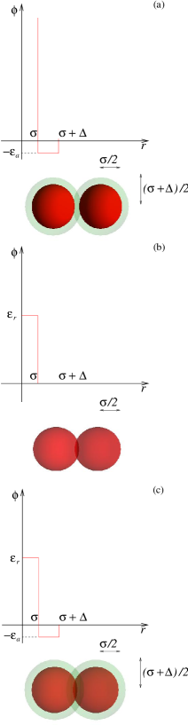
Figure 1: Sketch of the PSW potential used in the present work (c). This potential interpolates between the SW potential (a) and of the PS potential (b). In the SW case (a), spherical particles have a perfect steric hindrance of size $\sigma$ (the particle diameter) and attractive interactions of range $\sigma+\Delta$ highlighted as a halo in the picture. In the PS case (b), nearest-neighbor particles can partially interpenetrate, with some energy cost $\epsilon_{r}$, but have no attractive tail. In the PSW there is both the possibility of partial interpenetration (with cost $\epsilon_{r}$) and short-range SW attraction (with energy gain $\epsilon_{a}$).

In order to put the PSW model in perspective, let us briefly summarize the main features of the SW and PS potentials.

The SW model has a standard phase diagram typical of a simple fluid, with a fluid-fluid and a fluid-solid transitions in the intermediate range between the triple and the critical points in the temperature-density plane. The fluid-fluid transition becomes metastable, against crystallization, if the width of the well goes below a certain value that has been estimated to be $\Delta\approx 0.25\sigma$ Liu05 .

The PS fluid, on the other hand, does not display any fluid-fluid coexistence, in view of the lack of any attractive interactions. The fluid-solid transition is, however, possible and highly unconventional with the formation of multiple occupancy crystals coupled with possible reentrant melting in the presence of a smoother repulsive interaction, such as a Gaussian form Mladek08 ; Klein94 .

The PSW fluid combines features belonging to both limiting cases within a very subtle interplay between the repulsive and attractive energy scale that affects its thermodynamic stability Santos08 ; Fantoni09 ; Fantoni10a .

III Ruelle’s stability criterion

The issue of thermodynamic stability has a long and venerable history, dating back to the late sixties Fisher66 , and it is nicely summarized in Ruelle’s textbook that is a standard reference for this problem Ruelle69 .

A system is defined to be (Ruelle) thermodynamically stable Ruelle69 ; Fisher66 if there exists a positive number $B$, such that for the total potential energy ${\Phi}_{N}$ for a system of $N$ particles it holds

$${\Phi}_{N}\geq-NB.$$ (5)

The physical rationale behind this mathematical statement is that the ratio $-{\Phi}_{N}/N$ cannot grow unboundly as $N$ increases if the system is to be well behaving, but must converge to a well defined limit. This is usually referred to as Ruelle’s stability criterion.

Consider the PSW fluid. As density increases and temperature decreases, particles tend to lump together into clusters (“blobs”) as they pay some energetic price set by $\epsilon_{r}$ but they gain a (typically larger) advantage due to the attraction $\epsilon_{a}$. Therefore, as the ratio $\epsilon_{a}/\epsilon_{r}$ increases, one might expect to reach an unstable regime with very few clusters including a large number of significantly overlapping particles, so that ${\Phi}_{N}$ is no longer proportional to $N$.

The ratio $\epsilon_{a}/\epsilon_{r}$ (“penetrability”) plays in PSW fluids a very important role, as we shall see in the following sections. In Ref. Fantoni10a we proved that the one-dimensional (1D) PSW fluid satisfies Ruelle’s criterion if $\epsilon_{a}/\epsilon_{r}\leq 1/2(\ell+1)$, where $\ell$ is the integer part of $\Delta/\sigma$. In this case, we are then guaranteed to have a well defined equilibrium state.

Here we show that this result can be extended to a three-dimensional (3D) PSW fluid in that Ruelle’s criterion is satisfied if $\epsilon_{a}/\epsilon_{r}\leq 1/f_{\Delta}$, where $f_{\Delta}$ is the maximum number of non-overlapping particles that can be geometrically arranged around a given one within a distance between $\sigma$ and $\sigma+\Delta$. Of course, $f_{\Delta}$ depends on the width of the attractive interaction $\Delta$. For $\Delta/\sigma<\sqrt{2}-1$, for instance, one has $f_{\Delta}=12$, corresponding to a HCP closed packed configuration. In the following, we will use a generic $d$-dimensional notation and consider $d=3$ at the end.

The total potential energy of a PSW fluid formed by particles at positions $\mathbf{r}_{1},\ldots,\mathbf{r}_{N}$ can be written in general as

$${\Phi}_{N}\left(\mathbf{r}_{1},\ldots,\mathbf{r}_{N}\right)=\frac{1}{2}\sum_{i=1}^{N}\sum_{j\neq i}^{N}\phi\left(\left|\mathbf{r}_{i}-\mathbf{r}_{j}\right|\right)$$ (6)

Consider now such a configuration where particles are distributed in $M$ clusters along each direction, each made of $s$ perfectly overlapped particles, and with different clusters arranged in the close-packed configuration. In the Appendix we prove that indeed this is the lowest possible energy configuration in the two-dimensional (2D) case.

The total number of particles is $N=M^{d}s$. As clusters are in a close-packed configuration, particles of a given cluster interact attractively with all the particles of those $f_{\Delta}$ clusters within a distance smaller than $\sigma+\Delta$. Consequently, the potential energy has the form

$${{\Phi}_{N}(M)=\frac{1}{2}M^{d}s\left(s-1\right)\epsilon_{r}-\frac{M^{d}}{2}\left[{f_{\Delta}}-b_{\Delta}(M)\right]s^{2}\epsilon_{a}.}$$ (7)

The first term represents the repulsive energy between all possible pairs of particles in a given $s$-cluster, while the second term represents the attractive energy between clusters. Here $b_{\Delta}(M)$ accounts for a reduction of the actual number of clusters interacting attractively, due to boundary effects. This quantity clearly depends upon the chosen value of $\Delta/\sigma$ but we can infer the following general properties

$${b_{\Delta}(1)=f_{\Delta},\qquad b_{\Delta}(M>2)<f_{\Delta},\qquad\lim_{M\to\infty}b_{\Delta}(M)=0.}$$ (8)

In the 1D (with $\Delta/\sigma<1$) and 2D (with $\Delta/\sigma<\sqrt{3}-1$) cases, ${\Phi}_{N}(M)$ is given by Eqs. (19) and (26), respectively, so that $b_{\Delta}(M)=2M^{-1}$ (1D) and $b_{\Delta}(M)=2(4M^{-1}-M^{-2})$ (2D). In general, $b_{\Delta}(M)$ must be a positive definite polynomial of degree $d$ in $M^{-1}$ with no independent term, its form becoming more complicated as $d$ increases. However, we need not specify the actual form of $b_{\Delta}(M)$ for our argument, but only the properties given in Eq. (8).

Eliminating $s=N/M^{d}$ in favor of $M$ in Eq. (7) one easily gets

$$\frac{{\Phi}_{N}(M)}{N}=-\frac{\epsilon_{r}}{2}+\frac{N}{2}\epsilon_{a}M^{-d}F(M),$$ (9)

where we have introduced the function

$${F(M)\equiv b_{\Delta}(M)-\left(f_{\Delta}-\frac{\epsilon_{r}}{\epsilon_{a}}\right).}$$ (10)

Note that $F(M)$ is independent of $N$. If ${\epsilon_{a}}/{\epsilon_{r}}<1/f_{\Delta}$, $F(M)$ is positive definite and so ${\Phi}_{N}/N$ has a lower bound ($-\epsilon_{r}/2$) and the system is stable in the thermodynamic limit. Let us suppose now that ${\epsilon_{a}}/{\epsilon_{r}}>1/f_{\Delta}$. In that case, $F(1)={\epsilon_{r}}/{\epsilon_{a}}>0$ but $\lim_{M\to\infty}F(M)=-(f_{\Delta}-{\epsilon_{r}}/{\epsilon_{a}})<0$. Therefore, there must exist a certain finite value $M=M_{0}$ such that $F(M)<0$ for $M>M_{0}$. In the 1D (with $\Delta/\sigma<1$) and 2D (with $\Delta/\sigma<\sqrt{3}-1$) cases the values of $M_{0}$ can be explicitly computed:

$$M_{0} = \left(1-\frac{\epsilon_{r}}{2\epsilon_{a}}\right)^{-1},\quad(d=1),$$ (11)

$$M_{0} = \frac{2+\sqrt{1+{\epsilon_{r}}/{2\epsilon_{a}}}}{3}\left(1-\frac{\epsilon_{r}}{6\epsilon_{a}}\right)^{-1},\quad(d=2).$$ (12)

In general, it is reasonable to expect that $M_{0}\sim\left(1-{\epsilon_{r}}/{f_{\Delta}\epsilon_{a}}\right)^{-1}$. Regardless of the precise value of $M_{0}$, we have that $\lim_{N\to\infty}[-{\Phi}_{N}(M)]/N=\infty$ for $M>M_{0}$ and thus the criterion (5) is violated.

This completes the proof that, if ${\epsilon_{a}}/{\epsilon_{r}}<1/f_{\Delta}$, the system is thermodynamically stable as it satisfies Ruelle’s stability criterion, Eq. (5). Reciprocally, if ${\epsilon_{a}}/{\epsilon_{r}}>1/f_{\Delta}$ there exists a class of blob configurations violating Eq. (5). In those configurations the $N$ particles are concentrated on a finite (i.e., independent of $N$) number of clusters, each with a number of particles proportional to $N$. For large $N$ the potential energy scales with $N^{2}$ and thus the system exhibits non-extensive properties.

In three dimensions, $f_{\Delta}=12$, $18$, and $42$ if $\Delta/\sigma<\sqrt{2}-1$, $\sqrt{2}-1<\Delta/\sigma<\sqrt{3}-1$, and $\sqrt{3}-1<\Delta/\sigma<1$, respectively, and so the threshold values are ${\epsilon_{a}}/{\epsilon_{r}}=1/12$, $1/18$, and $1/42$, respectively. There might (and do) exist local configurations with higher coordination numbers, but only those filling the whole space have to be considered in the thermodynamic limit.

In general, Ruelle’s criterion (5) is a sufficient but not necessary condition for thermodynamic stability. Therefore, in principle, if $\epsilon_{a}/\epsilon_{r}>1/f_{\Delta}$ the system may or may not be stable, depending on the physical state (density $\rho$ and temperature $T$). However, compelling arguments discussed in Ref. Ruelle69 show that the PSW system with $\epsilon_{a}/\epsilon_{r}>1/f_{\Delta}$ is indeed unstable (i.e., non-extensive) in the thermodynamic limit for any $\rho$ and $T$. Notwithstanding this, even if $\epsilon_{a}/\epsilon_{r}>1/f_{\Delta}$, the system may exhibit “normal” (i.e., extensive) properties at finite $N$, provided the temperature is sufficiently high and/or the density is sufficiently low. It is therefore interesting to investigate this regime with the specific goals of (i) defining the stability boundary (if any) and (ii) outlining the fate of the SW-like fluid-fluid and fluid-solid lines as penetrability increases. This will be discussed in the next section, starting from the fluid-fluid coexistence lines.

IV Effect of penetrability on the fluid-fluid coexistence

We have performed an extensive analysis of the fluid-fluid phase transition of the three-dimensional PSW fluid by Gibbs Ensemble Monte Carlo (GEMC) simulations Frenkel96 ; Panagiotopoulos87 ; Panagiotopoulos88 ; Smit89a ; Smit89b . In all cases we have started with the SW fluid ($\epsilon_{a}/\epsilon_{r}=0$) and gradually increased penetrability $\epsilon_{a}/\epsilon_{r}$ until disappearance of the transition. Following standard prescriptions Frenkel96 ; Panagiotopoulos87 ; Panagiotopoulos88 ; Smit89a ; Smit89b , we construct the fluid-fluid coexistence lines using two systems (the gas and the liquid) that can exchange both volume and particles in such a way that the total volume $V$ and the total number of particles $N$ are fixed and the pressure and chemical potential coincide in both systems. $N=512$ particles were used. By denoting with $L_{i}$ and $V_{i}$ ($i=v,l$) the respective sizes and volumes of the vapor and liquid boxes, we used $2N$ particle random displacements of magnitude $0.15L_{i}$, $N/10$ random volume changes of magnitude $0.1$ in $\ln[V_{i}/(V-V_{i})]$, and $N$ particle swaps between the gas and the liquid boxes, on average per cycle.

Our code fully reproduces the results of Vega et al. Vega92 for the SW fluid, as further discussed below.

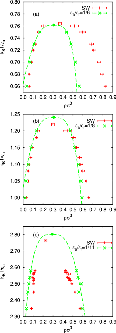
Figure 2: Fluid-fluid coexistence lines for different well widths $\Delta/\sigma$ and penetrabilities $\epsilon_{a}/\epsilon_{r}$. The SW results are those by Vega et al. Vega92 for the same value of $\Delta/\sigma$. Circles and boxes represent the estimated critical points for the PSW and the SW fluids, respectively, and the dotted lines represent the coexistence curves for the PSW case. (a) $\Delta/\sigma=0.25$ and $\epsilon_{a}/\epsilon_{r}=1/6$; (b) $\Delta/\sigma=0.5$ and $\epsilon_{a}/\epsilon_{r}=1/8$; (c) $\Delta/\sigma=1$ and $\epsilon_{a}/\epsilon_{r}=1/11$.

Figure 2 depicts some representative examples of the effect of penetrability on the SW results at different well widths $\Delta/\sigma$. As $\Delta/\sigma$ increases, the upper limit set by Ruelle’s stability condition $\epsilon_{a}/\epsilon_{r}\leq 1/f_{\Delta}$ decreases, and lower penetrability values $\epsilon_{a}/\epsilon_{r}$ have to be used to ensure the existence of the transition line. In Fig. 2, values $\epsilon_{a}/\epsilon_{r}=1/6,1/8,1/11$ were used for $\Delta/\sigma=0.25,0.5,1$, respectively. Figure 2 also includes an estimate of the critical points for the PSW fluid obtained from the law of rectilinear diameters, as discussed in Ref. Vega92 , that is

$$\frac{\rho_{l}+\rho_{v}}{2}=\rho_{c}+A(T_{c}-T)~{},$$ (13)

where $\rho_{l}$ ($\rho_{v}$) is the density of the liquid (vapor) phase, $\rho_{c}$ the critical density and $T_{c}$ the critical temperature. Furthermore, the temperature dependence of the density difference of the coexisting phases is fitted to the following scaling form

$$\rho_{l}-\rho_{g}=B(T_{c}-T)^{\beta}~{},$$ (14)

where the critical exponent for the three-dimensional Ising model $\beta=0.32$ was used to match the universal fluctuations. Amplitudes $A$ and $B$ where determined from the fit.

A detailed collection of the results corresponding to Fig. 2(a), (b), and (c) is reported in Table 1.

$\Delta/\sigma=0.25$, $\epsilon_{a}/\epsilon_{r}=1/6$
$k_{B}T/\epsilon_{a}$	$\rho_{v}\sigma^{3}$	$\rho_{l}\sigma^{3}$	$u_{v}/\epsilon_{a}$	$u_{l}/\epsilon_{a}$	$\mu_{v}-k_{B}T\ln\Lambda^{3}$	$\mu_{l}-k_{B}T\ln\Lambda^{3}$
$0.66$	$0.0377(6)$	$0.5634(6)$	$-0.343(8)$	$-3.441(13)$	$-2.410(7)$	$-2.51(12)$
$0.70$	$0.0724(15)$	$0.5256(15)$	$-0.614(16)$	$-3.100(13)$	$-2.253(5)$	$-2.27(6)$
$0.73$	$0.1093(45)$	$0.4805(42)$	$-0.862(38)$	$-2.920(45)$	$-2.157(12)$	$-2.29(8)$
$0.75$	$0.1684(95)$	$0.4368(95)$	$-1.204(67)$	$-2.682(27)$	$-2.211(8)$	$-2.01(2)$

$\Delta/\sigma=0.5$, $\epsilon_{a}/\epsilon_{r}=1/8$
$k_{B}T/\epsilon_{a}$	$\rho_{v}\sigma^{3}$	$\rho_{l}\sigma^{3}$	$u_{v}/\epsilon_{a}$	$u_{l}/\epsilon_{a}$	$\mu_{v}-k_{B}T\ln\Lambda^{3}$	$\mu_{l}-k_{B}T\ln\Lambda^{3}$
$1.00$	$0.0194(4)$	$0.5900(7)$	$-0.254(7)$	$-4.687(9)$	$-4.19(2)$	$-4.16(5)$
$1.05$	$0.0319(5)$	$0.5841(17)$	$-0.400(9)$	$-4.603(14)$	$-4.00(1)$	$-4.01(3)$
$1.10$	$0.0529(8)$	$0.5557(8)$	$-0.651(14)$	$-4.365(6)$	$-3.832(6)$	$-3.83(4)$
$1.15$	$0.0799(15)$	$0.5173(17)$	$-0.934(18)$	$-4.087(15)$	$-3.726(7)$	$-3.76(4)$
$1.20$	$0.1342(37)$	$0.4728(40)$	$-1.464(40)$	$-3.777(26)$	$-3.642(6)$	$-3.64(2)$

$\Delta/\sigma=1.0$, $\epsilon_{a}/\epsilon_{r}=1/11$
$k_{B}T/\epsilon_{a}$	$\rho_{v}\sigma^{3}$	$\rho_{l}\sigma^{3}$	$u_{v}/\epsilon_{a}$	$u_{l}/\epsilon_{a}$	$\mu_{v}-k_{B}T\ln\Lambda^{3}$	$\mu_{l}-k_{B}T\ln\Lambda^{3}$
$2.35$	$0.0327(4)$	$0.5920(11)$	$-0.693(8)$	$-8.931(12)$	$-8.90(2)$	$-8.87(6)$
$2.45$	$0.0476(5)$	$0.5593(16)$	$-1.004(11)$	$-8.439(21)$	$-8.66(1)$	$-8.61(3)$
$2.50$	$0.0577(8)$	$0.5844(12)$	$-1.201(17)$	$-8.653(17)$	$-8.54(2)$	$-8.59(5)$
$2.54$	$0.0670(12)$	$0.5511(37)$	$-1.377(25)$	$-8.231(42)$	$-8.48(2)$	$-8.51(2)$
$2.58$	$0.0769(9)$	$0.5361(19)$	$-1.556(20)$	$-8.030(22)$	$-8.41(1)$	$-8.38(3)$

Table 1: Vapor-liquid coexistence data from GEMC of $N=512$ PSW particles with $\Delta/\sigma=0.25$ and $\epsilon_{a}/\epsilon_{r}=1/6$ (top table), $\Delta/\sigma=0.5$ and $\epsilon_{a}/\epsilon_{r}=1/8$ (central table) and $\Delta/\sigma=1.0$ and $\epsilon_{a}/\epsilon_{r}=1/11$ (bottom table). We used $10^{7}$ MC steps. $T$, $\rho_{i}$, $u_{i}$, $\mu_{i}$ are, respectively, the temperature, the density, the internal energy per particle, and the chemical potential of the vapor ($i=v$) or liquid ($i=l$) phase ($\Lambda$ being the thermal de Broglie wavelength). Numbers in parentheses correspond to the error on the last digits. The estimated critical points are $k_{B}T_{c}/\epsilon_{a}=0.762$ and $\rho_{c}\sigma^{3}=0.307$.(top table), $k_{B}T_{c}/\epsilon_{a}=1.241$ and $\rho_{c}\sigma^{3}=0.307$ (central table) and $k_{B}T_{c}/\epsilon_{a}=2.803$ and $\rho_{c}\sigma^{3}=0.292$ (bottom table)

Note that seemingly stable transition curves are found in all representative cases depicted in Fig. 2, thus suggesting a “normal” fluid behavior for the finite-size system studied. Increasing penetrability $\epsilon_{a}/\epsilon_{r}$ at fixed $\Delta/\sigma$ progressively destabilize the transition, until a threshold value $(\epsilon_{a}/\epsilon_{r})_{\text{th}}$ is reached where no fluid-fluid transition is observed. Upon changing $\Delta/\sigma$, one can then draw a line of this values in the $\epsilon_{a}/\epsilon_{r}$ and $\Delta/\sigma$ plane. This is depicted in Fig. 3, where the instability line $(\epsilon_{a}/\epsilon_{r})_{\text{th}}$ is found to decrease as $\Delta/\sigma$ increases, thus gradually reducing the region where the fluid-fluid transition can be observed, as expected. The shadowed stepwise region identifies the thermodynamically stable region, as guaranteed by Ruelle’s criterion $\epsilon_{a}/\epsilon_{r}\leq 1/f_{\Delta}$ discussed above. Note that points $(\Delta/\sigma=0.25,\epsilon_{a}/\epsilon_{r}=1/6)$, $(\Delta/\sigma=0.5,\epsilon_{a}/\epsilon_{r}=1/8)$, and $(\Delta/\sigma=1,\epsilon_{a}/\epsilon_{r}=1/11$), corresponding to the values used in Fig. 2 and highlighted by circles, lie in the $1/f_{\Delta}\leq\epsilon_{a}/\epsilon_{r}\leq(\epsilon_{a}/\epsilon_{r})_{\text{th}}$ region, that is, outside the stable range guaranteed by Ruelle’s criterion.

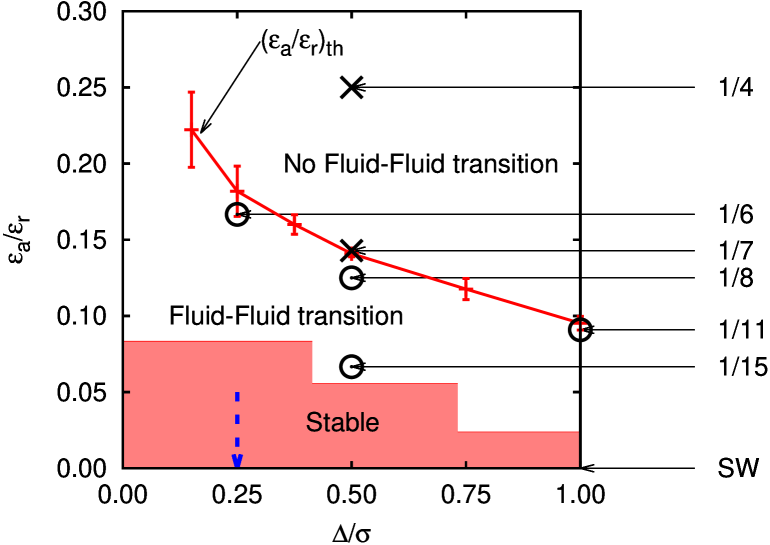
Figure 3: Plot of penetrability $\epsilon_{a}/\epsilon_{r}$ as a function of $\Delta/\sigma$. The displayed $(\epsilon_{a}/\epsilon_{r})_{\text{th}}$ line separates the parameter region where the PSW model, with $N=512$, admits a fluid-fluid phase transition (below this line) from that where it does not. The shadowed stepwise line highlights the region ($\epsilon_{a}/\epsilon_{r}\leq 1/12$ for $\Delta/\sigma<\sqrt{2}-1$, $\epsilon_{a}/\epsilon_{r}\leq 1/18$ for $\sqrt{2}-1<\Delta/\sigma<\sqrt{3}-1$, and $\epsilon_{a}/\epsilon_{r}\leq 1/42$ for $\sqrt{3}-1<\Delta/\sigma<1$) where the model is guaranteed to be thermodynamically stable for any thermodynamic state by Ruelle’s criterion. The SW model falls on the $\epsilon_{a}/\epsilon_{r}=0$ axis (with finite $k_{B}T/\epsilon_{a}$). The vertical dashed arrow points to the SW value $\Delta/\sigma\lesssim 0.25$ below which the fluid-fluid transition becomes metastable against the freezing transition Liu05 . The circles are the points chosen for the calculation of the coexistence lines (Figs. 2 and 9), while the crosses are the points chosen for the determination of the boundary phases discussed in Figs. 5 and 6.

V Stable, unstable, and metastable phases

Interestingly, in Ruelle’s textbook Ruelle69 , the three-dimensional PSW model corresponding to point $(\Delta/\sigma=1,\epsilon_{a}/\epsilon_{r}=1/11$) is exploited as an example of “catastrophic” fluid (see especially Fig. 4 and proposition 3.2.2 both in Ref. Ruelle69 ). This is clearly because this state point lies outside the stable region identified by Ruelle’s criterion, as discussed. As already remarked, however, this criterion does not necessarily imply that outside this region the system has to be unstable, but only that it is “likely” to be so. There are then two possibilities. First, that in the intermediate region $1/f_{\Delta}\leq\epsilon_{a}/\epsilon_{r}\leq(\epsilon_{a}/\epsilon_{r})_{\text{th}}$ the system is indeed stable in the thermodynamic limit, a case that is not covered by Ruelle’s criterion. Numerical results reported in Figs. 2 and 3 appear to support this possibility. The second possibility is that, even in this region, the system is strictly unstable, in the thermodynamic limit, but it appears to be a “normal” fluid when considered at finite $N$. This possibility cannot be ruled out by any simulation at finite $N$, and would be more plausible as hinted by Ruelle’s arguments.

In order to illustrate the fact that, at finite $N$, the system in the intermediate region $1/f_{\Delta}\leq\epsilon_{a}/\epsilon_{r}\leq(\epsilon_{a}/\epsilon_{r})_{\text{th}}$ behaves as a normal fluid, in Fig. 4 we show two representative snapshots of the gas and the liquid phases at the point $(\Delta/\sigma=0.5,\epsilon_{a}/\epsilon_{r}=1/8)$ that lies just below the $(\epsilon_{a}/\epsilon_{r})_{\text{th}}$ line (see Fig. 3). In both the gas and the liquid phases, the structure of the fluid presents the typical features of a standard SW fluid, with no significant overlap among different particles.

On the other hand, we have observed that above the threshold line $(\epsilon_{a}/\epsilon_{r})_{\text{th}}$ of Fig. 3, at a temperature close to the critical temperature of the corresponding SW system, the GEMC simulation evolves towards an empty box and a collapsed configuration in the liquid box.

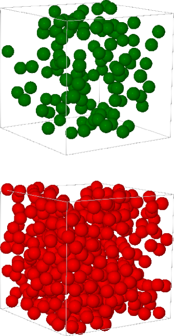
Figure 4: Two GEMC simulation snapshots ($N=512$) at $\Delta/\sigma=0.5$, $\epsilon_{a}/\epsilon_{r}=1/8$ (below the threshold value) and $k_{B}T/\epsilon_{a}=1.20$. The one on the top panel corresponds to the gas phase ($\rho_{v}\sigma^{3}=0.1342$), and the one on the bottom to the liquid phase ($\rho_{l}\sigma^{3}=0.4728$).

The second scenario described above can be supported or disproved by a finite-size study of the $N$-dependence of the transition, as described below.

Assume that at any finite $N$, the absolute minimum of the internal energy corresponds to the “collapsed” non-extensive configurations, referred to as “blob phase” in the following. As discussed in section III, the internal energy of these configurations scales with $N^{2}$ for large $N$. However, the system presumably also includes a large number of “normal” configurations with an internal energy that scales linearly with $N$. This will be referred to as “normal phase”.

There is then an energy gap between the total energy associated with the normal and the collapsed configurations with an energy ratio of order $N$. For finite $N$ and sufficiently high temperature, the Boltzmann statistical factor $e^{-{\Phi}_{N}/k_{B}T}$ of the collapsed configurations (in spite of the gap) might be not sufficiently large to compensate for the fact that the volume in phase space corresponding to normal configurations has a much larger measure (and hence entropy) than that corresponding to collapsed configurations. As a consequence, the physical properties look like normal and one observes a normal phase. Normal configurations have a higher internal energy but also may have a larger entropy. If $N$ is sufficiently small and/or $T$ is high enough, normal configurations might then have a smaller free energy than collapsed configurations. On the other hand, the situation is reversed at larger $N$ and finite temperature, where the statistical weight (i.e., the interplay between the Boltzmann factor and the measure of the phase space volume) of the collapsed configurations becomes comparable to (or even larger than) that of the normal configurations and physical properties become anomalous. This effect could be avoided only if $T$ grows (roughly proportional to $N$) as $N$ increases, since entropy increases more slowly with $N$ than $\Phi_{N}$.

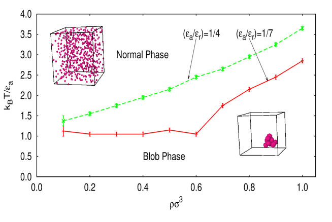
Figure 5: Regions of the phase diagram where the PSW fluid, with $\Delta/\sigma=0.5$ and two different values of $\epsilon_{a}/\epsilon_{r}$, is expected to exhibit a normal phase (above the instability line) or a blob phase (below the instability line) for $N=512$ particles. Note that the instability line corresponding to the higher penetrability case ($\epsilon_{a}/\epsilon_{r}=1/4$, dashed line) lies above the one corresponding to the lower penetrability ($\epsilon_{a}/\epsilon_{r}=1/7$, solid line). The two insets depict representative snapshots of respective typical configurations.

In a PSW fluid above the stable region ($\epsilon_{a}/\epsilon_{r}>1/f_{\Delta}$), we have then to discriminate whether the system is truly stable in the thermodynamic limit $N\to\infty$, or it is metastable, evolving into an unstable blob phase at a given value of $N$ depending on temperature and density.

In order to shed some more light into this dual metastable/unstable scenario, we performed NVT Monte Carlo simulations using $N=512$ particles initially distributed uniformly within the simulation box (“regular” initial condition). We carefully monitored the total potential energy of the fluid during the simulation and found that, at any given density, there exists a certain temperature $T_{\text{ins}}(\rho)$, such that the system behaves normally after $10^{7}N$ single particle moves (normal phase) if $T>T_{\text{ins}}$ and collapses to a few clusters of overlapped particles (blob phase) for $T<T_{\text{ins}}$.

This is shown in Fig. 5 for $\Delta/\sigma=0.5$ and two different penetrability values: $\epsilon_{a}/\epsilon_{r}=1/4$ (upper dashed line) and $\epsilon_{a}/\epsilon_{r}=1/7$ (lower solid line). The first value lies deeply in the instability region above the threshold $(\epsilon_{a}/\epsilon_{r})_{\text{th}}$ value of Fig. 3, while the second is sitting right on its top, for this value $\Delta/\sigma=0.5$ of the well width. Also depicted are two snapshots of two representative configurations found under these conditions. While the particles in the normal phase, $T>T_{\text{ins}}$, are arranged in a disordered configuration that spans the whole box (see upper snapshot of Fig. 5), one can clearly see that for $T<T_{\text{ins}}$ a “blob” structure has nucleated around a certain point within the simulation box with a few droplets of several particles each (see lower snapshot of Fig. 5).

The three fluid-fluid coexistence phase diagrams displayed in Fig. 2 are then representative of a metastable normal phase that persists, for a given $N$, up to $(\epsilon_{a}/\epsilon_{r})_{\text{th}}$ as long as the corresponding critical point $(\rho_{c},T_{c})$ is such that $T_{c}>T_{\text{ins}}(\rho_{c})$, as in the cases reported in Fig. 2. Below this instability line, the fluid becomes unstable at any density and a blob phase, where a few large clusters nucleate around certain points and occupy only a part of the simulation, is found. The number of clusters decreases (and the number of particles per cluster increases) as one moves away from the boundary line found in Fig. 5 towards lower temperatures. Here a cluster is defined topologically as follows. Two particles belong to the same cluster if there is a path connecting them, where we are allowed to move on a path going from one particle to another if the centers of the two particles are at a distance less than $\sigma$.

These results, while not definitive, are strongly suggestive of the fact that even the normal phase is in fact metastable and becomes eventually unstable in the $N\to\infty$ limit.

This can be further supported by a finite size scaling analysis at increasing $N$, as reported in Fig. 6 in the higher penetrability (and hence most demanding) case $\epsilon_{a}/\epsilon_{r}=1/4$.

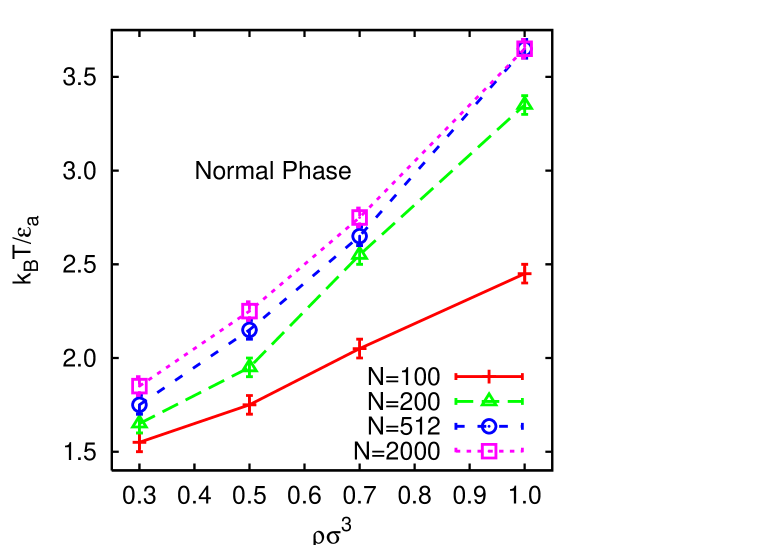
Figure 6: Size dependence of the instability line of Fig. 5 for the system $\epsilon_{a}/\epsilon_{r}=1/4$ and $\Delta/\sigma=0.5$.

In obtaining these results, we used NVT simulations with $10^{10}$ single particle moves in all cases.

As expected, the instability temperature line $T_{\text{ins}}(\rho)$ moves to higher values as $N$ increases, at fixed density $\rho\sigma^{3}$, from $N=100$ to $N=2000$, and the normal phase region significantly shrinks accordingly, being expected to vanish in the thermodynamic limit $N\to\infty$.

As said before, in all the above computations we started with a regular initial condition having all particles randomly distributed in the entire available simulation box. Under these circumstances, for $T<T_{\text{ins}}$ (where all particles are confined into a blob of a few clusters) a large number of MC steps is required in order to find the true equilibrium distribution. On the other hand, if we have a clustered configuration to start with, a much higher “melting” temperature $T_{\text{ins}}$, above which one recovers a normal phase, is expected. This “hysteresis” effect is indeed observed, as detailed below.

For $\epsilon_{a}/\epsilon_{r}=1/7$, $\Delta/\sigma=0.5$, and $\rho\sigma^{3}=1.0$ the normal-to-blob transition occurs upon cooling at $k_{B}T/\epsilon_{a}\approx 2.75$. Inserting the obtained configuration back in the MC simulation as an initial condition, and increasing the temperature, we find the blob phase to persist up to much higher temperatures $k_{B}T/\epsilon_{a}\approx 4$. The hysteresis is also found to be strongly size dependent. With the same system $\epsilon_{a}/\epsilon_{r}=1/7$, $\Delta/\sigma=0.5$, but for $\rho\sigma^{3}=0.6$, we found the blob-to-normal melting temperatures to be $k_{B}T/\epsilon_{a}=2$–$3$ for $N=256$, $k_{B}T/\epsilon_{a}=4$–$5$ for $N=512$, and $k_{B}T/\epsilon_{a}=6$-$7$ for $N=1024$. Analogously, in the state $\epsilon_{a}/\epsilon_{r}=1/4$, $\Delta/\sigma=0.5$, and $\rho\sigma^{3}=0.3$, the results are $k_{B}T/\epsilon_{a}=2.1$–$2.2$, $k_{B}T/\epsilon_{a}=3.7$–$3.8$, $k_{B}T/\epsilon_{a}=9.0$–$9.1$, and $k_{B}T/\epsilon_{a}=31$–$32$ for $N=100$, $N=200$, $N=512$, and $N=2000$, respectively.

In the interpretation of the size dependence of the hysteresis in the melting, one should also consider the fact that the blob occupies only part of the simulation box and therefore a surface term has a rather high impact on the melting temperature.

Additional insights on the sudden structural change occurring on the fluid upon crossing the threshold line $(\epsilon_{a}/\epsilon_{r})_{\text{th}}$ can be obtained by considering the radial distribution function (RDF) $g(r)$ tenWolde96 on two state points above and below this line. We consider a state point at $\Delta/\sigma=0.5$, $k_{B}T/\epsilon_{a}=1.20$, and $\rho\sigma^{3}=0.7$ and evaluate the RDF at $\epsilon_{a}/\epsilon_{r}=1/8$ (slightly below the threshold line, see Fig. 3) and at $\epsilon_{a}/\epsilon_{r}=1/7$. The latter case is sitting right on the top of the threshold line, according to Fig. 3. The results are depicted in Fig. 7.

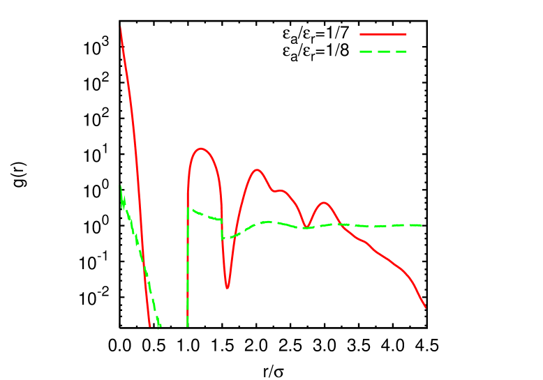
Figure 7: Radial distribution function for the PSW model at $\Delta/\sigma=0.5$, $k_{B}T/\epsilon_{a}=1.20$, and $\rho\sigma^{3}=0.7$ for two different values of the penetrability parameter $\epsilon_{a}/\epsilon_{r}$: $\epsilon_{a}/\epsilon_{r}=1/8$ (lying below the threshold line given in Fig. 3) and $\epsilon_{a}/\epsilon_{r}=1/7$ (that is on the top of it). The $g(r)$ axis is in a log scale.

Drastic changes in the structural properties of the PSW liquid are clearly noticeable. While in the normal phase ($\epsilon_{a}/\epsilon_{r}=1/8$) the RDF presents the typical features of a standard fluid for a soft-potential and, in particular, converges to unity, in the blob phase ($\epsilon_{a}/\epsilon_{r}=1/7$), the RDF presents a huge peak (note the log-scale) at $r=0$ and decays to zero after the first few peaks, a behavior that is suggestive of clustering and confinement of the system. The amplitude of the first maximum in the structure factor grows past the value of $2.85$, which is typically reckoned for an indication for a freezing occurring in the system, according to Ref. Hansen69 .

As a further characterization of the structural ordering of the system, we have also investigated a set of rotationally invariant local order indicators that have been often exploited to quantify order in crystalline solids, liquids, and colloidal gels tenWolde96 :

$$Q_{l}=\sqrt{\frac{4\pi}{2l+1}\sum_{m=-l}^{l}\left|\bar{Q}_{lm}\right|^{2}}~{},$$ (15)

where $\bar{Q}_{lm}$ is defined as

$$\bar{Q}_{lm}=\frac{\sum_{i=1}^{N_{c}}N_{b}(i)\bar{q}_{lm}(i)}{\sum_{i=1}^{N_{c}}N_{b}(i)}~{},$$ (16)

where $N_{c}$ is the number of clusters and

$$\bar{q}_{lm}\left(i\right)=\frac{1}{N_{b}\left(i\right)}\sum_{j=1}^{N_{b}\left(i\right)}Y_{lm}\left(\hat{\mathbf{r}}_{ij}\right)~{}.$$ (17)

Here $N_{b}(i)$ is the set of bonded neighbors of the $i$-th cluster, the unit vector $\hat{\mathbf{r}}_{ij}$ specifies the orientation of the bond between clusters $i$ and $j$, and $Y_{lm}(\hat{\mathbf{r}}_{ij})$ are the corresponding spherical harmonics.

A particularly useful probe of the possible crystal structure of the system is a value of $Q_{6}$ close to unity (see Appendix A of Ref. tenWolde96 ). Results for $Q_{6}$ from the PSW model are reported in Table 2 for the two values of penetrability considered in Fig. 5 ($\epsilon_{a}/\epsilon_{r}=1/4$ and $\epsilon_{a}/\epsilon_{r}=1/7$). In order to compute $Q_{6}$, the center of mass of each cluster (as topologically defined before) is identified. Then, the cutoff distance for the nearest-neighbors “bonds” is selected to be approximately equal to the second minimum of $g(r)$ ($r\approx 1.5\sigma$). As detailed in Table 2, we find $0.03\leq Q_{6}\leq 0.1$ for $\epsilon_{a}/\epsilon_{r}=1/4$ (top table) and $0.05\leq Q_{6}\leq 0.12$ for $\epsilon_{a}/\epsilon_{r}=1/7$ (bottom table), depending on the considered values of temperature and density. These values have been computed with $N=512$ particles but an increase up to $N=1024$ yields only a slight increase of $Q_{6}$.

$\epsilon_{a}/\epsilon_{r}=1/4$
$\rho\sigma^{3}$	$k_{B}T/\epsilon_{a}$	$N_{c}$	$Q_{6}$	$u/\epsilon_{a}$
0.1	1.0	13	0.04	-60
0.2	1.5	24	0.10	-57
0.3	1.7	115	0.03	-21
0.4	1.9	132	0.05	-19
0.5	2.1	116	0.05	-18
0.6	2.4	98	0.07	-19
0.7	2.6	84	0.04	-18
0.8	2.9	98	0.11	-19
0.9	3.2	74	0.09	-22
1.0	3.6	67	0.05	-23

$\epsilon_{a}/\epsilon_{r}=1/7$
$\rho\sigma^{3}$	$k_{B}T/\epsilon_{a}$	$N_{c}$	$Q_{6}$	$u/\epsilon_{a}$
0.1	1.0	51	0.12	-25
0.2	1.0	39	0.06	-37
0.3	1.0	41	0.05	-37
0.4	1.0	42	0.07	-33
0.5	1.1	50	0.29	-24
0.6	1.0	38	0.07	-36
0.7	1.7	55	0.05	-22
0.8	2.1	58	0.11	-22
0.9	2.4	60	0.06	-21
1.0	2.8	62	0.06	-21

Table 2: Number of clusters, $Q_{6}$ parameter, and internal energy per particle for the non-extensive phases found in the case $\Delta/\sigma=0.5$ and $\epsilon_{a}/\epsilon_{r}=1/4$ (top table) and $\epsilon_{a}/\epsilon_{r}=1/7$ (bottom table), just below the curves of Fig. 5. The parameter $Q_{6}$ was calculated on the final equilibrated particle configuration only, with a neighbor distance of $1.5\sigma$ in all cases.

Besides $Q_{6}$, in Table 2 we report other properties of the blob phases found with $\Delta/\sigma=0.5$ and $\epsilon_{a}/\epsilon_{r}=1/4$ and $\epsilon_{a}/\epsilon_{r}=1/7$, such as the number of clusters and the internal energy per particle $u/\epsilon_{a}$. We observe that the number of clusters is rather constant (typically $40$–$60$) for penetrability $\epsilon_{a}/\epsilon_{r}=1/7$. For the higher penetrability $\epsilon_{a}/\epsilon_{r}=1/4$ the number of clusters is generally larger, as expected, but is quite sensitive to the specific density and temperature values. As for the internal energy per particle, we observe that its magnitude is always more than four times larger than the kinetic contribution $\frac{3}{2}k_{B}T$.

No conclusive pattern appears from the analysis of results of Table 2, as there seems to be no well-defined behavior in any of the probes as functions of temperature and density, and this irregular behavior can be also checked by an explicit observation of the corresponding snapshots. Nonetheless, these results give no indications of the formation of any regular structure.

The final conclusion of the analysis of the fluid-fluid phase diagram region of the PSW model is that the system is strictly thermodynamically stable for $\epsilon_{a}/\epsilon_{r}<1/f_{\Delta}$ and strictly thermodynamically unstable above it, as dictated by Ruelle’s stability criterion. However, if $\epsilon_{a}/\epsilon_{r}>1/f_{\Delta}$ there exists an intermediate region where the system looks stable for finite $N$ and becomes increasingly unstable upon approaching the thermodynamic limit.

The next question we would like to address is whether this scenario persists in the fluid-solid transition, where already the PS model displays novel and interesting features. This is discussed in the next section.

VI The fluid-solid transition

It is instructive to contrast the expected phase diagram for the SW model with that of the PSW model.

Consider the SW system with a width $\Delta/\sigma=0.5$ that is a well-studied intermediate case where both a fluid-fluid and a fluid-solid transition have been observed Liu05 . The corresponding schematic phase diagram is displayed in Fig. 8 (top panel), where the critical point is $(k_{B}T_{c}/\epsilon_{a}=1.23,\rho_{c}\sigma^{3}=0.309)$ in the temperature-density plane, and its triple point is ($k_{B}T_{t}/\epsilon_{a}=0.508,P_{t}\sigma^{3}/\epsilon_{a}=0.00003)$ in the temperature-pressure plane, with $\rho_{l}\sigma^{3}=0.835$ and $\rho_{s}\sigma^{3}=1.28$ Liu05 . In Ref. Liu05 no solid stable phase was found for temperatures above the triple point, meaning that the melting curve in the pressure-temperature phase diagram is nearly vertical (see Fig. 8, top panel).

Figure 8: Schematic phase diagram of the SW fluid for $\Delta/\sigma=0.5$ (top panel) and phase diagram of the PSW fluid for $\Delta/\sigma=0.5$ and $\epsilon_{a}/\epsilon_{r}=1/8$ (bottom panel).

Motivated by previous findings in the fluid-fluid phase diagram, we consider the PSW model with $\Delta/\sigma=0.5$ and two different penetrability values $\epsilon_{a}/\epsilon_{r}=1/15$ and $\epsilon_{a}/\epsilon_{r}=1/8$ in the intermediate region $1/f_{\Delta}\leq\epsilon_{a}/\epsilon_{r}\leq(\epsilon_{a}/\epsilon_{r})_{\text{th}}$ (see Fig. 3), where one expects a normal behavior for finite $N$, but with different details depending on the chosen penetrability. In the present case, the first chosen value ($\epsilon_{a}/\epsilon_{r}=1/15$) lies very close the boundary ($\epsilon_{a}/\epsilon_{r}=1/f_{\Delta}$) of the stability region predicted by Ruelle’s criterion, whereas the second chosen value lies, quite on the contrary, close to the threshold curve $(\epsilon_{a}/\epsilon_{r})_{\text{th}}$.

We have studied the system by isothermal-isobaric (NPT) MC simulations, with a typical run consisting of $10^{8}$ MC steps (particle or volume moves) with an equilibration time of $10^{7}$ steps. We considered $N=108$ particles and adjusted the particle moves to have acceptance ratios of approximately $0.5$ and volume changes to have acceptance ratios of approximately $0.1$. Note that the typical relaxation time in the solid region is an order of magnitude higher than that of the liquid region.

Consider the case $\epsilon_{a}/\epsilon_{r}=1/8$ first. The result for the isotherm $k_{B}T/\epsilon_{a}=1$ is reported in Fig. 9, this temperature being smaller than the critical one $k_{B}T_{c}/\epsilon_{a}=1.241$. From this figure we can clearly see the jumps in the density corresponding to the gas-liquid coexistence region and to the liquid-solid coexistence region.

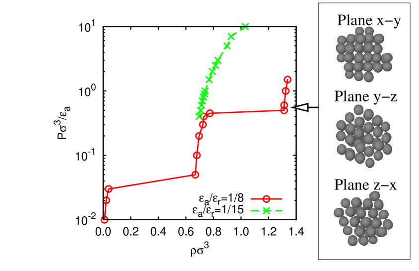
Figure 9: Isotherm $k_{B}T/\epsilon_{a}=1$ for the PSW system with $\Delta/\sigma=0.5$ and $\epsilon_{a}/\epsilon_{r}=1/8$ and $\epsilon_{a}/\epsilon_{r}=1/15$, as obtained from NPT MC simulations with $N=108$ particles. The pressure axis is in logarithmic scale. Three views of the same snapshot of the centers of mass of the clusters in the solid are shown on the right-hand side.

On the basis of the obtained results, we can foresee a phase diagram of the PSW system for this particular value of penetrability to be the one sketched in Fig. 8 (bottom panel). In particular, the melting curve has a positive slope in the pressure-temperature phase diagram, unlike the almost vertical slope of the SW counterpart, as discussed. This implies that penetrability allows for a “softening” of the liquid-solid transition, so the liquid and the solid can coexist at a temperature higher than the triple one without the need of a huge increase of pressure.

Next we also consider a fluid with $\epsilon_{a}/\epsilon_{r}=1/15$, just outside the Ruelle stability region, at the same temperature as before. The results are also reported in Fig. 8 and show no indications of a stable solid in the considered range of pressures, in agreement with the fact that at this very low value of penetrability the behavior of the system is very close to the SW counterpart.

A specific interesting peculiarity of the PSW system in the intermediate region $1/f_{\Delta}\leq\epsilon_{a}/\epsilon_{r}\leq(\epsilon_{a}/\epsilon_{r})_{\text{th}}$ of Fig. 3 is a lack of full consistency with known thermodynamic relations. In this case, in fact, unlike the SW counterpart, we were unable to trace the coexistence curve between the liquid and the solid using Kofke’s method Kofke93a ; Kofke93b , which is equivalent to the numerical integration of the Clausius–Clapeyron equation

$$\left(\frac{d\ln P}{d\beta}\right)_{c}=-\frac{\Delta h}{\beta P\Delta v},\quad\beta\equiv\frac{1}{k_{B}T},$$ (18)

with $\Delta h=h_{l}-h_{s}$ and $\Delta v=v_{l}-v_{s}$, where $h_{i}$ and $v_{i}$ denote, respectively, the molar enthalpy and volume of phase $i$ ($i=l$ for the liquid phase and $i=s$ for the solid phase); the subscript $c$ indicates that the derivative is taken along the coexistence line. Once a single point on the coexistence curve between the two phases is known one can use a trapezoid integration scheme Kofke93b to integrate Eq. (18).

In our calculation, we have selected a penetrability $\epsilon_{a}/\epsilon_{r}=1/8$ and the isotherm of Fig. 8, $k_{B}T/\epsilon_{a}=1$, as a reference point. The coexistence pressure at that temperature is $P\sigma^{3}/\epsilon_{a}\approx 0.475$ and the molar volume jump is $\Delta v/\sigma^{3}\approx 1/0.775-1/1.313\approx 0.529$. We have then calculated the molar enthalpy in the NPT ensemble by computing $\langle PV+U\rangle/N$ (where $U$ is the total internal energy of the system) with the result $\Delta h/\epsilon_{a}\approx-5.042-(-7.593)=2.551$. Choosing a spacing in $\beta$ of $-0.05/\epsilon_{a}$ we get from Eq. (18) a predicted coexistence pressure $P\sigma^{3}/\epsilon_{a}\approx 0.789$ at $k_{B}T/\epsilon_{a}=1/0.95\simeq 1.053$. Instead, however, at the latter temperature we found the coexistence pressure between $0.5$ and $0.6$. Despite this quantitative discrepancy, Eq. (18) is useful to understand that the relatively mild slope of the PSW liquid-solid coexistence line in the pressure-temperature phase diagram is essentially due to the fact that the internal energies of the coexisting liquid and solid phases are not too disparate.

A close inspection of several snapshots of the obtained solid phase suggests that, in the intermediate penetrability case, the obtained crystal is made of clusters of overlapping particles located at the sites of a regular crystal lattice with $Q_{6}\approx 0.35$ tenWolde96 and a triclinic structure characterized by a unit cell of sides $a=b=c=\sigma$ and angles $\alpha=\beta=\pi/3$ and $\gamma=\cos^{-1}(1/4)$ (see three views of a common snapshot in Fig. 9).

It is worth stressing that the additional degree of penetrability, not present in the SW counterpart, is responsible for the coexistence of the liquid and the solid at not excessively large pressures. Clearly, we cannot rule out the possibility of other additional solid-solid coexistence regions at higher pressures.

VII Conclusions

In this paper, we have studied the phase diagram of the three-dimensional PSW model. This model combines penetrability, a feature typical of effective potential in complex fluids, with a square-well attractive tail, accounting for typical effective attractive interactions that are ubiquitous in soft matter. It can then be regarded as the simplest possible model smoothly interpolating between PS ($\epsilon_{a}/\epsilon_{r}\to 0$, $k_{B}T/\epsilon_{r}=\text{finite}$) and SW ($\epsilon_{a}/\epsilon_{r}\to 0$, $k_{B}T/\epsilon_{a}=\text{finite}$) fluids, as one changes penetrability $\epsilon_{a}/\epsilon_{r}$ and temperature.

We have proved that the model is thermodynamically stable when $\epsilon_{a}/\epsilon_{r}<1/f_{\Delta}$, as it satisfies Ruelle’s stability criterion Ruelle69 . Above this value, the fluid is, strictly speaking, unstable in the thermodynamic limit, exhibiting non-extensive properties. For finite $N$, however, it displays a rather rich and interesting phenomenology. In particular, there exists an intermediate region $1/f_{\Delta}\leq\epsilon_{a}/\epsilon_{r}\leq(\epsilon_{a}/\epsilon_{r})_{\text{th}}$ in the penetrability-width plane (see Fig. 3) where the fluid displays normal or anomalous behavior depending on the considered temperatures and densities. For sufficiently large temperatures ($T>T_{\text{ins}}(\rho)$) the fluid presents a metastable normal behavior with (apparently) stable liquid-liquid and liquid-solid transitions, provided the relative critical temperatures are above the instability line $T=T_{\text{ins}}$. In this case, we have studied the effect of penetrability on the fluid-fluid transition (see Fig. 2) close to the threshold line $(\epsilon_{a}/\epsilon_{r})_{\text{th}}$ and found that in general the transition has a higher critical temperature than the SW counterpart. We have attributed this result to the additional degree of freedom given by penetrability that tends to oppose the formation of a crystal until a sufficient large density is achieved.

Below the instability line $T_{\text{ins}}(\rho)$, however, different particles tend to overlap into a few isolated clusters (blobs) confined in a small portion of the available volume and the total energy does no longer scale linearly with the number of particles $N$. As a consequence, the fluid becomes thermodynamically unstable and its properties very anomalous (Fig. 5). The metastable region shrinks as either $\epsilon_{a}/\epsilon_{r}$ or $N$ increase (Fig. 6).

Above the threshold line $(\epsilon_{a}/\epsilon_{r})_{\text{th}}$ (see Fig. 3) the fluid-fluid coexistence disappears, since in this case $T_{\text{ins}}$ is too high to allow any phase-separation (for a given $N$).

An additional interesting feature of the metastable/unstable dualism is included in the hysteresis dependence on the initial condition. When the initial configuration is an unstable one (i.e., a blob) the system melts back to a normal phase at temperatures that are in generally significantly higher than those where the transition normal-to-blob is achieved upon cooling. We have attributed this behavior to the small statistical weight of the blob configuration in the Boltzmann sampling, in spite of its significantly larger energetic contribution.

We have also studied the fluid-solid transition in the intermediate metastable region $1/f_{\Delta}\leq\epsilon_{a}/\epsilon_{r}\leq(\epsilon_{a}/\epsilon_{r})_{\text{th}}$. We find that the solid density typically increases with respect to the corresponding SW case, due to the formation of clusters of overlapping particles in the crystal sites, as expected on physical grounds. The melting curve is found to have a relatively smooth positive slope, unlike the SW counterpart, and this anomalous behavior is also reflected in the thermodynamic inconsistency present in the Clausius–Clapeyron thermodynamic equation, thus confirming the metastable character of the phase. When penetrability is sufficiently low to be close to the Ruelle stable region, the system behaves as the corresponding SW system.

One might rightfully wonder whether the finite $N$ metastable phase presented here should have any experimental consequence at all. We believe the answer to be positive. Imagine to be able to craft, through a clever chemical synthesis process, a fluid that may be described by an effective interaction of the PSW form. Our work has then set the boundary for observing a very intriguing normal-to-collapsed phase by either tuning the temperature/density parameters, or by increasing the number of particles in the fluid. In this case, it is the finite $N$ state, rather than the true thermodynamic limit $N\to\infty$, the relevant one.

Appendix A Ruelle’s stability criterion in $d=2$

Let us consider the two-dimensional PSW model characterized by $\epsilon_{a}/\epsilon_{r}$ and $\Delta/\sigma<\sqrt{3}-1$. The latter condition implies that in a hexagonal close-packed configuration a particle can interact attractively only with its nearest neighbors, so that $f_{\Delta}=6$.

Given the number of particles $N$, we want to get the configuration with the minimum potential energy ${\Phi}_{N}$. We assume that such a configuration belongs to the class of configurations described by $m$ rows, each row made of $M$ clusters, each cluster made of $s$ perfectly overlapped particles. The centers of two adjacent clusters (in the same row or in adjacent rows) are separated a distance $\sigma$. The total number of particles is $N=mMs$. Figure 10 shows a sketch of a configuration with $m=4$ rows and $M=6$ clusters per row.

Figure 10: Sketch of a configuration with $m=4$ rows and $M=6$ clusters per row.

The potential energy of an individual row is the same as that of the one-dimensional case Santos08 , namely

$${\Phi}^{\text{row}}=Ms\frac{s-1}{2}\epsilon_{r}-\left(M-1\right)s^{2}\epsilon_{a}.$$ (19)

The first term accounts for the repulsive energy between all possible pairs of particles in a given $s$-cluster, while the second term accounts for attractions that are limited to nearest neighbors if $\Delta/\sigma<\sqrt{3}-1$ in $d=2$. The potential energy of the whole system is $m{\Phi}^{\text{row}}$ plus the attractive energy of nearest-neighbor clusters sitting on adjacent rows (and taking into account the special case of boundary rows). The result is

$${\Phi}_{N}(m,s) = m\left[Ms\frac{s-1}{2}\epsilon_{r}-\left(M-1\right)s^{2}\epsilon_{a}\right]-(m-1)\left[1+2(M-1)\right]s^{2}\epsilon_{a}$$ (20)

$$= N\frac{s-1}{2}\epsilon_{r}-\left[\frac{3m-2}{m}N-(2m-1)s\right]s\epsilon_{a}.$$

For a given number of rows $m$, the value of $s$ that minimizes ${\Phi}_{N}(m,s)$ is found to be

$$s_{*}(m) = N\frac{3m-2}{2m(2m-1)}\left[1-\frac{m}{2(3m-2)}\frac{\epsilon_{r}}{\epsilon_{a}}\right],$$ (21)

which is meaningful only if $\epsilon_{a}/\epsilon_{r}>m/2(3m-2)>1/6$. Otherwise, $s_{*}(m)=1$. Therefore, the corresponding minimum value is

$${\Phi}_{N}^{*}(m) \equiv {\Phi}_{N}(m,s_{*}(m))$$ (22)

$$= -\frac{N}{2}\epsilon_{r}\begin{cases}1+N\frac{(3m-2)^{2}}{2m^{2}(2m-1)}\frac{\epsilon_{a}}{\epsilon_{r}}\left[1-\frac{m}{2(3m-2)}\frac{\epsilon_{r}}{\epsilon_{a}}\right]^{2},&\frac{\epsilon_{a}}{\epsilon_{r}}>\frac{m}{2(3m-2)},\\ 2\left(\frac{3m-2}{m}-\frac{2m-1}{N}\right)\frac{\epsilon_{a}}{\epsilon_{r}},&\frac{\epsilon_{a}}{\epsilon_{r}}<\frac{m}{2(3m-2)}.\end{cases}$$

Let us first suppose that $\epsilon_{a}/\epsilon_{r}<1/6$. In that case, $\epsilon_{a}/\epsilon_{r}<m/2(3m-2)$ regardless of the value of $m\geq 1$ and, according to Eq. (22), the minimization of ${\Phi}_{N}^{*}(m)$ is achieved with $m=M=N^{1/2}$. As a consequence, Ruelle’s stability criterion (5) is satisfied in the thermodynamic limit with $B=3\epsilon_{a}$.

Let us now minimize ${\Phi}_{N}^{*}(m)$ with respect to $m$ if $\epsilon_{a}/\epsilon_{r}>m/2(3m-2)$. This yields the quadratic equation $(6-\epsilon_{r}/\epsilon_{a})m^{2}-12m+4=0$, whose solution is

$$m_{**}=\frac{2}{3-\sqrt{3+\epsilon_{r}/\epsilon_{a}}}.$$ (23)

The condition $\epsilon_{a}/\epsilon_{r}>m_{**}/2(3m_{**}-2)$ is easily seen to be equivalent to the condition $\epsilon_{a}/\epsilon_{r}>1/6$. Therefore, the absolute minimum of the potential energy in that case is

$${\Phi}_{N}^{**} \equiv {\Phi}_{N}^{*}(m_{**})$$ (24)

$$= -\frac{N}{2}\epsilon_{r}\left[1+\frac{N}{8}\frac{\epsilon_{a}}{\epsilon_{r}}\left(3-\sqrt{3+\epsilon_{r}/\epsilon_{a}}\right)^{3}\left(1+\sqrt{3+\epsilon_{r}/\epsilon_{a}}\right)\right].$$

The corresponding value of $s_{*}$ is

$$s_{**} \equiv s_{*}(m_{**})$$ (25)

$$= \frac{N}{4}\left(3-\sqrt{3+\epsilon_{r}/\epsilon_{a}}\right)^{2}.$$

Comparison between Eqs. (23) and (25) shows that $N=m_{**}^{2}s_{**}$, i.e., the number of clusters per row equals the number of rows, $M_{**}=m_{**}$, as might have anticipated by symmetry arguments.

Equation (24) shows that, if $\epsilon_{a}/\epsilon_{r}>1/6$, $\lim_{N\to\infty}(-{\Phi}_{N}^{**})/N=\infty$ and thus Ruelle’s stability condition (5) is not fulfilled.

We could have restricted to a symmetric arrangement from the very beginning, i.e., $m=M$ and $N=M^{2}s$, in which case Eq. (20) yields

$${\Phi}_{N}(M,s=N/M^{2}) = M^{2}s\frac{s-1}{2}\epsilon_{r}-\left(3M^{2}-4M+1\right)s^{2}\epsilon_{a}$$ (26)

$$= \frac{N}{2}\left(\frac{N}{M^{2}}-1\right)\epsilon_{r}-\left(3M^{2}-4{M}+1\right)\frac{N^{2}}{M^{4}}\epsilon_{a}.$$

The minimum value (if $\epsilon_{a}/\epsilon_{r}>1/6$) corresponds to the value $M=m_{**}$ given by Eq. (23), as expected.

References

- (1) C. N. Likos, Phys. Rep. 348, 267 (2001).
- (2) F. H. Stillinger, J. Chem. Phys. 65, 3968 (1976).
- (3) J. McCarty, I. Y. Lyubimov, and M. G. Guenza, Macromol. 43, 3964 (2010).
- (4) P. G. Bolhuis, A. A. Louis, J. P. Hansen, and E. J. Meijer, J. Chem. Phys. 114, 4296 (2001).
- (5) C. Marquest and T. A. Witten, J. Phys. (France) 50, 1267 (1989).
- (6) C. N. Likos, M. Watzlawek, and H. Löwen, Phys. Rev. E 58, 3135 (1998).
- (7) B. M. Mladek, P. Charbonneau, C. N. Likos, D. Frenkel, and G. Kahl, J. Phys.: Condens. Matter 20, 494245 (2008).
- (8) A. Santos, R. Fantoni, and A. Giacometti, Phys. Rev. E 77, 051206 (2008).
- (9) R. Fantoni, A. Giacometti, A. Malijevský, and A. Santos, J. Chem. Phys. 131, 124106 (2009).
- (10) R. Fantoni, A. Giacometti, A. Malijevský, and A. Santos, J. Chem. Phys. 133, 024101 (2010).
- (11) R. Fantoni, J. Stat. Mech., P07030 (2010).
- (12) D. Mukamel and H. A. Posch, J. Stat. Mech. P03014 (2009).
- (13) A. Giacometti, G. Pastore, and F. Lado, Mol. Phys. 107, 555 (2009).
- (14) L. Vega, E. de Miguel, L. F. Rull, G. Jackson, and I. A. McLure, J. Chem. Phys. 96, 2296 (1992).
- (15) E. de Miguel, Phys. Rev. E 55, 1347 (1997).
- (16) F. del Río, E. Ávalos, R. Espíndola, L. F. Rull, G. Jackson, and S. Lago, Mol. Phys. 100, 2531 (2002).
- (17) H. Liu, S. Garde, and S. Kumar, J. Chem. Phys. 123, 174505 (2005).
- (18) M. E. Fisher and D. Ruelle, J. Math. Phys. 7, 260 (1966).
- (19) D. Ruelle Statistical Mechanics: Rigorous Results, (Benjamin 1969); ch. 3.
- (20) R. Fantoni, A. Malijevský, A. Santos and A. Giacometti, Europhys. Lett. 93, 26002 (2011).
- (21) A. Malijevský and A. Santos, J. Chem. Phys. 124, 074508 (2006).
- (22) A. Malijevský, S. B. Yuste, and A. Santos, Phys. Rev. E 76, 021504 (2007).
- (23) W. Klein, H. Gould, R. A. Ramos, I. Clejan, and A. I. Mel’cuk, Physica A 205, 738 (1994).
- (24) D. Frenkel and B. Smit Understanding Molecular Simulation (Academic Press, London, 1996).
- (25) A. Z. Panagiotopoulos, Mol. Phys. 61, 813 (1987).
- (26) A. Z. Panagiotopoulos, N. Quirke, M. Stapleton, and D. J. Tildesley , Mol. Phys. 63, 527 (1988).
- (27) B. Smit, Ph. De Smedt, and D. Frenkel, Mol. Phys. 68, 931 (1989).
- (28) B. Smit and D. Frenkel, Mol. Phys. 68, 951 (1989).
- (29) P. R. ten Wolde, M. J. Ruiz-Montero, and D. Frenkel, J. Chem. Phys. 104, 9932 (1996).
- (30) J. P. Hansen and L. Verlet, Phys. Rev. 189, 151 (1969).
- (31) D. A. Kofke, Mol. Phys. 78, 1331 (1993).
- (32) D. A. Kofke, J. Chem. Phys. 98, 4149 (1993).