Abstract

A stochastic theory for a branching process in a neutron population with two energy levels is used to assess the applicability of the differential self-interrogation Feynman-alpha method by numerically estimated reaction intensities from Monte Carlo simulations. More specifically, the variance to mean or Feynman-alpha formula is applied to investigate the appearing exponentials using the numerically obtained reaction intensities.

1 Introduction

Energy dependent aspects of neutron counting have been used to detect and determine the content of nuclear materials for several decades. The prime application is the Differential Die-Away Analysis (DDAA) method [1, 2, 3, 4, 5]. It is a deterministic method in which the time dependence of the detection rate of fast neutrons, after that an initial pulse of fast neutrons is injected to the sample, is used to determine the presence of fissile materials such as ${}^{235}U$ and ${}^{239}Pu$. Its application is suitable when the fissile material is embedded in a moderating surroundings such that the source neutrons induce thermal fission after having slowed down.

The drawback of pulsed measurements such as the DDAA method is the necessity of the use of a neutron generator. The stochastic generalization of the DDAA method was recently suggested as an alternative method which eliminates the need for such an external source, namely the so-called Differential Die-away Self-Interrogation (DDSI) technique [6]. The DDSI method utilizes the inherent spontaneous neutron emission of the sample. In the absence of a trigger signal, the temporal decay of the correlations as a function of the time delay between two detections of fast neutrons is used in the DDSI method. This corresponds to a Rossi-alpha measurement with two energy groups.

In Ref. [6] the functional form of the DDSI formula, i.e. the two-group Rossi-alpha formula, was derived in an empirical way. This formula was therefore later derived from first principles with the use of backward-type Kolmogorov equations [7, 8]. A two-group theory of the Rossi- and Feynman alpha formulae is interesting also in areas other than nuclear safeguards, such as pulsed and stationary source driven experiments measuring the reactivity in fast cores of accelerator driven sub-critical systems. In such experiments it was found that two exponentials appear, indicating that the temporal behavior of the fast and thermal neutrons is separated, especially in fast reflected cores. This amplifies the need for the two group versions of the Feynman and Rossi-alpha formulae [7, 8].

In this contribution, a stochastic theory for a branching process in a neutron population with two energy levels is investigated based on the previous results of Refs [7, 8, 9]. In particular, a counterpart of the DDSI formula, the Differential Self-interrogation Variance to Mean or Feynman-alpha formula, which we shall call the DSVM formula, is derived by using the master equation or Kolmogorov forward approach. The model includes a spontaneous fission source of fast neutrons, absorption in both groups, down-scattering (removal) from the fast to the thermal group, thermal fission, and detection of fast neutrons.

Practical applicability of the method, which is based on the observation of two different exponentials, depends on the quantitative values of the various within- and inter-group neutron reaction intensities, which appear as coefficients in the equations. This is in contrast to the energy-independent theory of multiplicity where the only appearing parameter is the first collision probability. To assess the applicability and expected performance of the DSVM method in practical situations, the above mentioned reaction intensities were determined from numerical Monte Carlo (MCNP4c) simulations. Significance of different values of the reaction intensities of thermal and fast neutrons in the performance of the method is discussed.

2 A variance to mean formula for the detected fast neutrons

In this section we will briefly discuss the fundamentals of the derivation of the variance to mean or Feynman-alpha for the two particle type system by using the Kolmogorov forward approach following Ref. [9]. In the model we have included a compound Poisson source of fast neutrons described by the source strength $S_{1}$ that releases $n$ particles with probability $p_{q}(n)$ at an emission event (i.e. spontaneous fission). We have assumed that the source is switched on at time $t=t_{0}<0$, although the dependence on $t_{0}$ will not be denoted. The detection rate of particles is included and is denoted by the intensity $\lambda_{d}$. We will start by giving a presentation of the analytical model consisting of a differential equation for the probability $P(N_{1},N_{2},Z_{1},t)$ for having $N_{1}$ fast, $N_{2}$ thermal neutrons at time $t$ in the system and having detected $Z_{1}$ fast particles in the interval $(0,t)$. In deriving this differential equation we have summed all mutually exclusive events during an infinitesimally small time interval $dt$ and we find for the probability $P(N_{1},N_{2},Z_{1},t)$ the differential equation

$$\frac{\partial P(N_{1},N_{2},Z_{1},t)}{\partial t} = -(\lambda_{1}N_{1}+\lambda_{2}N_{2}+S_{1})P(N_{1},N_{2},Z_{1},t)$$ (1)

$$+ \lambda_{1a}(N_{1}+1)P(N_{1}+1,N_{2},Z_{1},t)$$

$$+ \lambda_{2a}(N_{2}+1)P(N_{1},N_{2}+1,Z_{1},t)$$

$$+ \lambda_{R}(N_{1}+1)P(N_{1}+1,N_{2}-1,Z_{1},t)$$

$$+ \lambda_{2f}(N_{2}+1)\sum_{k}^{N_{1}}f(k)P(N_{1}-k,N_{2}+1,Z_{1},t)$$

$$+ \lambda_{d}(N_{1}+1)P(N_{1}+1,N_{2},Z_{1}-1,t)$$

$$+ S_{1}\sum_{n}^{N_{1}}p_{q}(n)P(N_{1}-n,N_{2},Z_{1},t).$$

Here, $\lambda_{1}$ and $\lambda_{2}$ are the decay constants (total reaction intensities) for fast and thermal particles, whereas $\lambda_{1a}$, $\lambda_{2a}$ are the absorption (actually, capture) intensities of fast and thermal particles, respectively. The removal of fast particles into the thermal group is described by $\lambda_{R}$ while fission resulting from the thermal particles happens with the intensity of $\lambda_{2f}$. The total intensities are given by

$$\lambda_{1}=\lambda_{1a}+\lambda_{R}+\lambda_{d},$$ (2)

and

$$\lambda_{2}=\lambda_{2a}+\lambda_{2f}.$$ (3)

We derive the equations for the factorial moments by using the generating function of the form

$$G(X,Y,Z,t) = \sum_{N_{1}}\sum_{N_{2}}\sum_{Z_{1}}X^{N_{1}}Y^{N_{2}}Z^{Z_{1}}P(N_{1},N_{2},Z_{1},t),$$ (4)

and describe the time evolution of the process by a partial differential equation in terms of the generating function as,

$$\frac{\partial G}{\partial t} = (\lambda_{1a}+\lambda_{R}Y+\lambda_{d}Z-\lambda_{1}X)\frac{\partial G}{\partial X}+(\lambda_{2a}+\lambda_{2f}q(X)-\lambda_{2}Y)\frac{\partial G}{\partial Y}$$ (5)

$$+ S_{1}(r(X)-1)G,$$

where

$$q(X) = \sum_{k}f_{k}X^{k},\;\;\;\;\;\;\;\;\;\;\mbox{and}$$ (6)

$$r(X) = \sum_{n}p_{q}(n)X^{n}.$$ (7)

Here, $f_{k}$ is the probability of having exactly $k$ neutrons produced in an induced fission event. We have used the definition of the derivatives of the expressions (6) and (7) as $\nu_{1}=dq/dX|_{X=1}$ and $r_{1}=dh/dX|_{X=1}$, which stand for the expectations of the number of neutrons from induced and sponaneous fissions, respectively [10]. We note that for $t_{0}\rightarrow-\infty$, the expectations of fast neutrons ($\langle N_{1}\rangle$) and thermal neutrons ($\langle N_{2}\rangle$) will reach steady state due to the stationary source term with intensity $S_{1}$. The solutions to the system of differential equations are found by differentiation of equation (5) with respect to ($X,Y,Z$) and then letting ($X=Y=Z=1$). These read as

$$\langle N_{1}\rangle = \bar{N}_{1}=\frac{\lambda_{2}S_{1}r_{1}}{\lambda_{1}\lambda_{2}-\nu_{1}\lambda_{R}\lambda_{2f}}=\frac{\lambda_{2}S_{1}r_{1}}{\omega_{1}\omega_{2}},$$ (8)

$$\langle N_{2}\rangle = \bar{N}_{2}=\frac{\lambda_{R}S_{1}r_{1}}{\omega_{1}\omega_{2}},$$ (9)

$$\langle Z_{1}\rangle = \varepsilon\lambda_{2f}\bar{N}_{1}t,$$ (10)

where $\varepsilon=\lambda_{d}/\lambda_{2f}$ and we have used the additional definitions $\omega_{1}$ and $\omega_{2}$ and $\nu_{eff}$ as

$$-\omega_{1} = -\frac{1}{2}(\lambda_{1}+\lambda_{2})+\frac{1}{2}\sqrt{(\lambda_{1}-\lambda_{2})^{2}+4\lambda_{1}\lambda_{2}\nu_{eff}},$$ (11)

$$-\omega_{2} = -\frac{1}{2}(\lambda_{1}+\lambda_{2})-\frac{1}{2}\sqrt{(\lambda_{1}-\lambda_{2})^{2}+4\lambda_{1}\lambda_{2}\nu_{eff}},$$ (12)

$$\nu_{eff} = \nu_{1}\frac{\lambda_{R}\lambda_{2f}}{\lambda_{1}\lambda_{2}}.$$ (13)

It can be noted that in reactor physics terminology, $\nu_{eff}$ is identical with $k_{eff}$ of a multiplying system and that the expectation of the detections increases linearly with time. This is due to the fact that it is determined by integration of the expectation of the neutron number with respect to time. In order to find the variance of the detector counts we need to determine the second moments by yet another differentiation with respect to ($X,Y,Z$) followed by letting ($X=Y=Z=1$). We find the variance of the detector counts through the relation $\sigma_{Z}^{2}=\langle Z_{1}\rangle+\mu_{ZZ}$ where the modified variance $\mu_{ZZ}$ is defined as $\mu_{ZZ}=\langle Z(Z-1)\rangle-\langle Z\rangle^{2}=\sigma_{ZZ}^{2}-\langle Z\rangle$ while in general we have $\mu_{XY}=\langle XY\rangle-\langle X\rangle\langle Y\rangle$. The differentiation procedure results in a system of six ordinary differential equations for the second order modified moments. The differentiation procedure gives a system of six dynamical equations of the modified second moments as

$$\frac{\partial}{\partial t}\mu_{XX} = -2\lambda_{1}\mu_{XX}+2\nu_{1}\lambda_{2f}\mu_{XY}+\nu_{2}\lambda_{2f}\bar{N}_{2}+S_{1}r_{2},$$ (14)

$$\frac{\partial}{\partial t}\mu_{XY} = -(\lambda_{1}+\lambda_{2})\mu_{XY}+\lambda_{R}\mu_{XX}+\nu_{1}\lambda_{2f}\mu_{YY},$$ (15)

$$\frac{\partial}{\partial t}\mu_{YY} = -2\lambda_{2}\mu_{YY}+2\lambda_{R}\mu_{XY},$$ (16)

$$\frac{\partial}{\partial t}\mu_{ZX} = -\lambda_{1}\mu_{ZX}+\nu_{1}\lambda_{2f}\mu_{ZY}+\lambda_{d}\mu_{XX},$$ (17)

$$\frac{\partial}{\partial t}\mu_{ZY} = -\lambda_{2}\mu_{ZY}+\lambda_{R}\mu_{ZX}+\lambda_{d}\mu_{XY},$$ (18)

$$\frac{\partial}{\partial t}\mu_{ZZ} = 2\epsilon\lambda_{2f}\mu_{XZ},$$ (19)

The equation system and its solution is rather analogous to the case of the Feynman-alpha equations with one neutron energy group but including delayed neutrons, as given in Ref. [11]. Although an analytical solution for the general time-dependent system of equations (14) - (19) would be hard to find, we note that in the stationary state the system breaks down into two systems such that the solution of the first three equations is independent from the second, such that the moments $\langle\mu_{XX}\rangle=\bar{\mu}_{XX}$, $\langle\mu_{XY}\rangle=\bar{\mu}_{XY}$ and $\langle\mu_{YY}\rangle=\bar{\mu}_{YY}$ are constants. The equations describing detected particles need to be solved retaining the full time evolution by e.g. Laplace transforms. Moreover, it is found that the sought moment $\langle\mu_{ZZ}\rangle$ is determined by quadrature of moment $\langle\mu_{XZ}\rangle$. We find the constant 2nd moments as,

$$\bar{\mu}_{XX} = \frac{(\lambda_{2}^{2}+\omega_{1}\omega_{2})(\nu_{2}\lambda_{2f}\bar{N}_{2}+S_{1}r_{2})}{2(\lambda_{1}+\lambda_{2})\omega_{1}\omega_{2}},$$ (20)

$$\bar{\mu}_{XY} = \frac{\lambda_{2}\lambda_{R}(\nu_{2}\lambda_{2f}\bar{N}_{2}+S_{1}r_{2})}{2(\lambda_{1}+\lambda_{2})\omega_{1}\omega_{2}},$$ (21)

$$\bar{\mu}_{YY} = \frac{\lambda_{R}^{2}(\nu_{2}\lambda_{2f}\bar{N}_{2}+S_{1}r_{2})}{2(\lambda_{1}+\lambda_{2})\omega_{1}\omega_{2}}.$$ (22)

Here we have used the notations $\nu_{2}=d^{2}q/dX^{2}|_{X=1}$ and $r_{2}=d^{2}h/dX^{2}|_{X=1}$ for the second factorial moments [10]. The objective now is to solve (17) and (18) by Laplace transform methods and we find the transformed identity as,

$$\tilde{\mu}_{XZ}=\frac{\nu_{1}\lambda_{d}\lambda_{2f}\bar{\mu}_{XY}}{sH(s)}+\frac{(s+\lambda_{2})\lambda_{d}\bar{\mu}_{XX}}{sH(s)}$$ (23)

with

$$H(s)=s^{2}+(\omega_{2}+\omega_{1})s+\omega_{1}\omega_{2}.$$ (24)

Note that we have assumed that the initial values of the moments $\mu_{XZ}$ and $\mu_{YZ}$ were equal to zero at $t=0$ (at the start of the measurement), hence the roots of $H(s)$ determine the temporal behavior of the Feynman-alpha formula. Moreover, the solution has many similarities to that found in Ref. [11]. We determine the variance to mean or Feynman-alpha formula by utilizing the relation for the variance $\sigma_{ZZ}=\langle Z\rangle+\mu_{ZZ}$ and after some algebra we find,

$$\frac{\sigma_{ZZ}(T)}{\langle Z_{1}\rangle}=1+Y_{1}(1-\frac{1-e^{-\omega_{1}T}}{\omega_{1}T})+Y_{2}(1-\frac{1-e^{-\omega_{2}T}}{\omega_{2}T}).$$ (25)

Here, the complete expressions for $Y_{1}$ and $Y_{2}$ are quite lengthy. However, it turns out that the sum $Y_{0}=Y_{1}+Y_{2}$ takes a rather simple form that also determines the value of the Feynman-alpha for large measurement times $T\rightarrow\infty$ as,

$$Y_{0}=Y_{1}+Y_{2}=\nu_{2}\frac{\lambda_{d}\lambda_{2}\lambda_{R}\lambda_{2f}}{\omega_{1}^{2}\omega_{2}^{2}}.$$ (26)

In the next section we will consider some quantitative examples of the variance to mean formula in Equation (25).

3 Quantitative assessment of the variance to mean formula

We will now discuss the quantitative application of the variance to mean formula (25) for a MOX fuel assembly, considering setups when the MOX fuel was homogeneously mixed with a different amount of polyethylene moderator. The fuel sample was in form of a sphere which has the same amount of material as one single fuel pin, yielding a radius of 3.36 cm, of typical MOX fuel (U(94.14%)O2 + Pu(5.86%)O2) with approximately 4% fissile content. The amount of moderator mixed into the fuel was taken as that corresponding to an outer reflector shell of 4 different thicknesses: 5, 10, 15 and 20 cm. In all cases the neutron source was assumed in the sample centre. In addition, a case was considered where the source was assumed to be equally distributed in the volume (designated as VDS, Volume Distributed Source) with the amount of moderator corresponding to 5 cm thickness. The geometry of the calculations is displayed in the r.h.s. of Figure 1, whereas the l.h.s. of the Figure shows the equivalent heterogeneous model, displaying a surrounding moderator which was mixed homogeneously in the sample for the simulations. We have hence carried out five Monte-Carlo (MCNP4с) simulations [12] in order to estimate the reaction intensities in the spent fuel assemblies with varying amount of moderation where the radius is taken as fissile material + moderator ($3.36+d$ cm). In the simulations we have assumed a two energy group approximation with a $0.46$ eV energy cut-off. Moreover, the energies of the source neutrons were sampled from the Watt fission spectrum, originating from the spontaneous fission of ${}^{240}Pu$. The energy spectrum is determined by the function,

$$p(E)\sim e^{-E/a}\sinh(bE)^{1/2}$$ (27)

where $a=0.799$ MeV and $b=4.903$ $MeV^{-1}$.

Table 1: Simulation Results

Intensity	5 cm	10 cm	15 cm	20 cm	VDS
$\lambda_{1}$ $[1/s]$	1.560	1.230	0.625	0.185	1.490
$\lambda_{2}$ $[1/s]$	0.637	1.220	1.260	1.180	0.325
$\lambda_{R}$ $[1/s]$	0.450	0.621	0.391	0.094	0.452
$\lambda_{2f}$ $[1/s]$	0.243	0.285	0.171	0.094	0.118

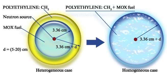
Figure 1: Show the geometry used for the Monte Carlo (MCNP4c) simulations for the homogenized cases (left figure showing fuel mixed with different amounts of polyethylene moderator) compared to the heterogeneous cases (right).

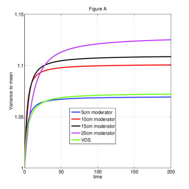
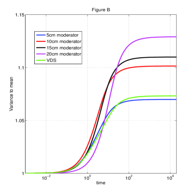
Figure 2: (A and B) The Feynman-alpha formula is shown for the cases generated by Monte Carlo (MCNP4c) simulations with 5-20 cm moderator in lin-lin scale (Figure A) and lin-log scale (Figure B).

The simulation results are shown in Table 1 for the cases described above. The reaction intensities obtained from the simulations were normalized to one starting neutron and are obtained with a relative error less than 1%. The resulting reaction intensities are used in the variance-to-mean expression in Eq. (25) and the results are displayed in Figures 2 A and B. In Figure 2A, the variance to mean in lin-lin scale is shown for the parameters in Table 1 whereas the remaining parameters are $\nu_{1}=2.87$, $\nu_{2}=4.635$, $\lambda_{d}=0.1$, $r_{1}=1.0$ and $r_{2}=0.0$. We find that that the difference between the variance to mean for the volume distributed source (VDS in table (1), green line) and the point source with 5 cm moderator (blue line) is very small indicating that the point source model is sufficient for describing the system. We note that the values of $\nu_{eff}$ are 0.316, 0.338, 0.244, 0.116 and 0.316 for the cases with 5 cm, 10 cm, 15 cm, 20 cm moderator and the VDS, respectively. In Figure 2B the variance to mean from Figure 2A is displayed in lin-log scale using the same parameter values as in Figure 2A. The reaction intensities of the moderated cases are approximately of the same order of magnitude and thus the two exponentials are not easily distinguished.

4 Discussion and conclusions

We have developed a forward Kolmogorov approach for the two group theory of the Differential Die-Away Self Interrogation Variance to Mean (DSVM), including a compound Poisson source and the detection process. The results agree with those calculated by the backward approach as reported in [7, 8]. We have used Monte Carlo simulations to find the reaction intensities needed to quantitatively assess the DSVM formula. We find that, unlike in the DDSI method (i.e. the two-group version of the Rossi-alpha method), the presence of two exponents in the solution is most often not clearly visible. This means that detection of the presence of fissile material may not be as obvious as with the Rossi-alpha method. By using the two group Rossi-alpha expression 4.34 in Ref. [7], we find the reverse situation, where in most cases with moderator the two exponentials appear. On the other hand, the determination of the exponents $\omega_{1}$ and $\omega_{2}$ by curve fitting could be more accurate in certain cases than with the DDSI method. Elucidating on the diagnostic value of the exponents in terms of determination of the sample parameters is not clear yet, and it requires further investigations, which will be reported in future work.

5 Acknowledgements

This work was supported by the Swedish Radiation Safety Authority (SSM).

References

- [1] W. Kunz, J. T. Caldwell, J. D. Atencuo, Apparatus and method for quantitative assay of generic transuranic wastes from nuclear reactors., US Patent 4,483,816, March (1982)
- [2] S. Croft, B. Mc Elroy, L. Bourva, M. Villani, WM R03 Conf. Proc. (2003)
- [3] K. A. Jordan, Detection of Special Nuclear Material in Hydrogenous Cargo Using Differential Die-Away Analysis, PhD Thesis, Dept. Nucl. Engineering, University of California, Berkeley (2006)
- [4] K. A Jordan, T. Gozani, Nucl. Instr. and Meth. B 261, 365 (2007)
- [5] K. A Jordan, T. Gozani, J. Vujic, Nucl. Instr. and Meth. A 598, 436 (2008)
- [6] H.O. Menlove, S.H. Menlove and S.T. Tobin, Nucl. Instr. and Meth. A 602 588 2009
- [7] L. Pál and I. Pázsit, Eur. Phys. J. Plus 126:20 (2011).
- [8] I. Pázsit and L. Pál, A stochastic model of the differential die-away analysis (DDAA) method, Proceedings 51st INMM 11 - 15 July, Baltimore, USA (2010)
- [9] J. Anderson, I. Pázsit and L. Pál, On the Feynman-alpha formula for fast neutrons, Poceedings 33rd ESARDA 16-20 May, Budapest, Hungary (2011)
- [10] I. Pázsit and L. Pál, “Neutron Fluctuations - a Treatise on the Physics of Branching Processes”. Elsevier Ltd, Oxford New York Tokyo (2008)
- [11] I. Pázsit and Y. Yamane, Ann. Nucl. Energy, Vol. 25, No. 9, 667 (1998)
- [12] J. F. Breismeister Ed., MCNP, General Monte Carlo N-Particle Transport Code, Version 4С, Los Alamos National Laboratory Report, LA - 12625 (1995).