Pre–Main-Sequence stellar populations across Shapley Constellation III.
I. Photometric Analysis and Identification

Abstract

We present our investigation of pre–main-sequence (PMS) stellar populations in the Large Magellanic Cloud (LMC) from imaging with Hubble Space Telescope WFPC2 camera. Our targets of interest are four star-forming regions located at the periphery of the super-giant shell LMC 4 (Shapley Constellation III). The PMS stellar content of the regions is revealed through the differential Hess diagrams and the observed color-magnitude diagrams (CMDs). Further statistical analysis of stellar distributions along cross-sections of the faint part of the CMDs allowed the quantitative assessment of the PMS stars census, and the isolation of faint PMS stars as the true low-mass stellar members of the regions. These distributions are found to be well represented by a double Gaussian function, the first component of which represents the main-sequence field stars and the second the native PMS stars of each region. Based on this result, a cluster membership probability was assigned to each PMS star according to its CMD position. The higher extinction in the region LH 88 did not allow the unambiguous identification of its native stellar population. The CMD distributions of the PMS stars with the highest membership probability in the regions LH 60, LH 63 and LH 72 exhibit an extraordinary similarity among the regions, suggesting that these stars share common characteristics, as well as common recent star formation history. Considering that the regions are located at different areas of the edge of LMC 4, this finding suggests that star formation along the super-giant shell may have occurred almost simultaneously.

1. Introduction

Considerable star formation in the Large Magellanic Cloud (LMC) takes place in interstellar shells, ranging from small bubbles to large super-giant shells (see, e.g., Chu, 2009). Among the latter, LMC 4 (Meaburn, 1980) is the largest super-giant shell in the Local Group, encompassing a remarkable Hi cavity of diameter $\sim$ 1.9 kpc (Dopita, Mathewson, & Ford, 1985). Centered on Shapley Constellation III (Shapley, 1951) the area of LMC 4 comprises over 500 clusters, associations and emission nebulae (Bica et al., 1999). In the Milky Way, the youngest stellar associations with $\tau<10$ Myr are surrounded by bright Hii regions, and comprise high-mass main sequence (MS) stars as well as intermediate- and low-mass pre-main sequence (PMS) stars. While the high-mass (OB-type) MS and intermediate-mass (Herbig Ae/Be) PMS populations are the direct signature of the youthfulness of their hosting associations, the low-mass PMS stars preserve a record of the complete recent star formation history of the region over long periods, since their evolution is extremely slow and can last up to many tens of Myr. Bearing this in mind, we undertake a research project that aims at a comprehensive study of the stellar populations in LMC star-forming regions, with emphasis on the recent star formation history in the vicinity of LMC 4 as recorded in the low-mass PMS populations.

Table 1Description of the WFPC2 observations within our HST Program GO-11547.

Association	Visit	R.A.	Decl.	Data set	Filter	Exposure	Observation
(Field)	No	(J2000.0)	(J2000.0)	filename		time (s)	Date
LH 63	1	05h27m47$.\!\!^{\rm s}$91	$-$67∘25′43$.\!\!^{\prime\prime}$0	ub0h010	F300W	$1\times~{}10$, $6\times 160$	2008 Jul 15
					F450W	$1\times~{}10$, $6\times 160$	2008 Jul 15
					F555W	$4\times 300$, $2\times 350$	2008 Jul 15
					F656N	$1\times 300$, $1\times 260$, $1\times 800$	2008 Jul 15
					F814W	$4\times 260$, $2\times 300$	2008 Jul 15
	2	05h28m05$.\!\!^{\rm s}$60	$-$67∘25′35$.\!\!^{\prime\prime}$1	ub0h020	F555W	$4\times 300$, $2\times 350$	2008 Jul 19
					F814W	$4\times 260$, $2\times 300$	2008 Jul 19
LH 60	3	05h27m10$.\!\!^{\rm s}$89	$-$67∘27′27$.\!\!^{\prime\prime}$3	ub0h030	F300W	$1\times~{}10$, $6\times 160$	2008 Jul 18
					F450W	$1\times~{}10$, $6\times 160$	2008 Jul 18
					F555W	$4\times 300$, $2\times 350$	2008 Jul 18
					F656N	$1\times 300$, $1\times 260$, $1\times 800$	2008 Jul 18
					F814W	$4\times 260$, $2\times 300$	2008 Jul 18
	4	05h27m28$.\!\!^{\rm s}$56	$-$67∘27′19$.\!\!^{\prime\prime}$4	ub0h040	F555W	$4\times 300$, $2\times 350$	2008 Jul 19
					F814W	$4\times 260$, $2\times 300$	2008 Jul 19
LH 72	5	05h32m26$.\!\!^{\rm s}$03	$-$66∘28′15$.\!\!^{\prime\prime}$8	ub0h050	F300W	$1\times~{}10$, $6\times 160$	2008 Jul 21
					F450W	$1\times~{}10$, $6\times 160$	2008 Jul 21
					F555W	$4\times 300$, $2\times 350$	2008 Jul 21
					F656N	$1\times 300$, $1\times 260$, $1\times 800$	2008 Jul 21
					F814W	$4\times 260$, $2\times 300$	2008 Jul 21
	6	05h32m08$.\!\!^{\rm s}$59	$-$66∘28′24$.\!\!^{\prime\prime}$0	ub0h060	F555W	$4\times 300$, $2\times 350$	2008 Jul 14
					F814W	$4\times 260$, $2\times 300$	2008 Jul 14
LH 88	7	05h35m55$.\!\!^{\rm s}$13	$-$67∘34′39$.\!\!^{\prime\prime}$9	ub0h570	F300W	$1\times~{}10$, $6\times 160$	2008 Sep 1
					F450W	$1\times~{}10$, $6\times 160$	2008 Sep 1
					F555W	$4\times 300$, $2\times 350$	2008 Sep 1
					F656N	$1\times 300$, $1\times 260$, $1\times 800$	2008 Sep 1
					F814W	$4\times 260$, $2\times 300$	2008 Sep 1
	8	05h35m37$.\!\!^{\rm s}$72	$-$67∘34′50$.\!\!^{\prime\prime}$5	ub0h080	F555W	$4\times 300$, $2\times 350$	2008 Jul 9
					F814W	$4\times 260$, $2\times 300$	2008 Jul 9
Field 1		05h41m38$.\!\!^{\rm s}$52	$-$68∘17′01$.\!\!^{\prime\prime}$8	u9e5550	F555W	$2\times 500$	2008 Feb 21
					F814W	$2\times 500$	2008 Feb 21
Field 2		05h24m04$.\!\!^{\rm s}$72	$-$67∘21′57$.\!\!^{\prime\prime}$7	u9px070	F555W	$2\times 500$	2007 May 20
					F814W	$2\times 500$	2007 May 20

Note. — Observations of Fields 1 and 2, for the assessment of the general LMC field population, are observed within HST programs GO-10583 (PI: C. Stubbs) and GO-10903 (PI: A. Rest) respectively. These data were retrieved from the HST Data Archive.

The existence of such stars in star-forming regions of the LMC became recently known thanks to the angular resolution and wide-field coverage provided by Hubble Space Telescope (HST). Archival images taken with the Wide-Field Planetary Camera 2 (WFPC2) of the young LMC association LH 52 (Lucke & Hodge, 1970), located at the northeastern edge of LMC 4, revealed for the first time that low-mass PMS stars can be directly identified in the color-magnitude diagram (CMD) from photometry in $V$- and $I$-equivalent filters (Gouliermis, Brandner, & Henning, 2006). While the WFPC2 images of LH 52 provided the first proof of the existence of such young stars in LMC star-forming regions, they were not deep enough to allow a statistically sound investigation of these stars. Subsequent deep photometry with the Advanced Camera for Surveys (ACS) in the same filters of the association LH 95, located at the northwest periphery of LMC 4, revealed an outstanding sample of more than 2,500 low-mass PMS stars down to the (model-dependent) mass-limit of $\sim$ 0.2 M_⊙, the smallest stellar mass ever observed in another galaxy (Gouliermis et al., 2007).

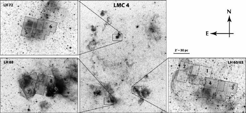
Figure 1.— Maps of the regions observed. The general area of the super-giant shell LMC 4 is shown in the center from a scanned UK Schmidt telescope plate observed in the $R$ band, available from the DSS. The extracted subregions, shown on the left and right of the figure, cover about 10^′ $\times$ 7^′ around the targets. The observed WFPC2 pointings are overlaid and annotated according to the corresponding visit number (see also Table 1). The scale indicator corresponds to the fields-of-view of the individual regions around the observed clusters. The field-of-view of the image of the general LMC 4 area is $\sim$ 1.7^∘ $\times$ 2.2^∘ (about 1.5 kpc $\times$ 2 kpc).

These data are characterized by an unprecedented completeness in their photometry due to their deepness. They provided us, thus, a unique sample of PMS stars, which we utilized to address in detail the formation of a young stellar cluster in another galaxy. Specifically, we addressed the initial mass function (IMF) of LH 95 down to the sub-solar regime (Da Rio, Gouliermis, & Henning, 2009) and the age of the cluster, as well as the duration of the star formation process in it, via the detection of an age-spread among its low-mass PMS stars (Da Rio, Gouliermis, & Gennaro, 2010). The aforementioned investigations provide a unique insight of the faintest stars in two star-forming regions within LMC 4. However, a more complete analysis of PMS populations in this area requires the collection of data on a larger sample of such objects. Within our HST program GO-11547 we obtained multi-band imaging of four additional star-forming regions located at the periphery of LMC 4 in order to accomplish a thorough characterization of PMS, MS and evolved stars in their vicinity, study their formation process, determine the stellar IMF and its variations in different environments, and provide an ample set of physical parameters of all observed stellar types in these regions.

In this first paper we present the photometry, identify the low-mass PMS stellar populations in the observed regions, and determine their cluster membership via their CMD positions. Specifically, in § 2 we present the observations of this program and describe the photometric process, as well as its accuracy and completeness. Our measurements of the interstellar reddening towards the targets, based on the photometry of the brighter MS stars, are presented in § 3. We present the observed CMDs in § 4, where we also discuss the CMD of the general LMC field. The identification and a qualitative assessment of the PMS stars in the observed regions takes place in § 5, where the Hess diagrams and a Monte Carlo technique for the statistical subtraction of field stars from the observed CMDs are described. In § 6 we present the quantitative determination of the true PMS populations of the observed regions from the stellar distributions along cross-sections of the observed CMDs. We discuss our findings in § 7. Concluding remarks and our plans for subsequent analyses are given in § 8.

2. Observations and Photometry

2.1. Observations

Our investigation is based on the analysis of data collected within our HST program GO-11547 (PI: D. Gouliermis) that imaged young stellar clusters located at the apparent edge of the super-giant shell LMC 4. Our targets are the young associations LH 60, LH 63, LH 72 and LH 88 (Lucke & Hodge, 1970), embedded in the bright emission nebulae DEM L 201, 228 and 241 (Davies, Elliott, & Meaburn, 1976), coinciding with the Hii regions LHA 120-N 51A,C, N 55A and N 59C (Henize, 1956), respectively. Maps of the general region of LMC 4 and the immediate areas of the targets are shown in Fig. 1. As such star-forming regions extend to sizes up to a few 10 pc (1^′ $\simeq$ 15 pc at the distance of the LMC), our investigation requires the best combination of high angular resolution, to overcome crowding effects for faint stars, and wide field-of-view to effectively sample each region. During Cycle 16 the most appropriate instrument for this task was WFPC2. To achieve large spatial coverage each cluster was observed with two overlapping pointings. The first pointing was centered on the brightest part of the associated Hii region and WFPC2 imaging was performed in the broad-band filters F300W, F450W, F555W, F814W and the narrow-band filter F656N, roughly equivalent to standard $U$, $B$, $V$, $I$ and H$\alpha$, respectively. We refer to each of these first group of multi-band pointings on the Hii regions as Pointing 1. The second WFPC2 pointings of each cluster, referred to as Pointing 2, are centered off the bright nebula and were observed only in the F555W and F814W filters.

Since we wish to eliminate confusion effects, especially for the detection of the low-mass PMS populations, all observations are performed with a suitable dithering, using a sub-pixel pointing pattern, in order to improve the spatial resolution. Furthermore, long exposures were split into intervals to aid in the removal of cosmic rays without any significant cost in the $S/N$ of the final combined image. Short exposures in the F300W and F450W filters are used to obtain photometry for the brightest and youngest stars in these regions. Previous ground-based photometry is also available for these stars (e.g., Hill, Madore, & Freedman, 1994; Olsen, Kim, & Buss, 2001). The consideration of the guide star acquisition, reacquisition of the telescope, and the instrument overhead times (e.g., change of filter, CCD readout, dithering) resulted in one set of four orbits for each Pointing 1 and two orbits for each Pointing 2. The orbits for each pointing were grouped as a visit, for a total of 8 visits using a total of 24 orbits (Fig. 2). A detailed summary of the observations is given in Table 1. For the assessment of the stellar populations in the general field of the LMC in the vicinity of the observed systems we used WFPC2 observations of the LMC field available in the HST Data Archive. We retrieved and analyzed images obtained in two campaigns, observed with parameters similar to ours. Details about these data are given also in Table 1.

Figure is omitted due to size limitations.

Copy available upon request to the first author.

Figure 2.— Color composite images of the primary WFPC2 observations of our program GO-11547 constructed from the reduced images taken in the filters F555W (blue) and F814W (red). Top panel shows all Pointings 1, i.e., visits 1, 3, 5, and 7. Bottom panel shows the Pointings 2, i.e., visits 2, 4, 6, and 8. The corresponding cluster names are also given.

Table 2Statistics on stars detected in filter-pairs with our photometry in each of Pointings 1.

	F300W	F450W	F555W	F814W	F656N
LH 63
F300W	579	565	453	515	418
F450W		2 538	2 389	2 464	500
F555W			5 027	4 869	394
F814W				5 753	452
F656N					559
LH 60
F300W	348	340	294	316	257
F450W		2 509	2 436	2 467	357
F555W			5 237	5 050	309
F814W				5 551	332
F656N					409
LH 72
F300W	445	435	362	401	282
F450W		2 022	1 920	1 963	344
F555W			3 801	3 698	264
F814W				4 493	306
F656N					421
LH 88
F300W	206	201	173	180	141
F450W		1 777	1 719	1 737	229
F555W			3 819	3 715	201
F814W				4 321	207
F656N					285

2.2. Photometry

Photometry is performed using the package HSTphot (Ver. 1.1) specifically designed for WFPC2 imaging (Dolphin, 2000). HSTphot is tailored to handle the undersampled nature of the point-spread function (PSF) in WFPC2 images and uses a self-consistent treatment of the charge transfer efficiency (CTE) and zero-point photometric calibrations. This package has the ability to perform photometry simultaneously for all exposures in different filters. Another advantage of HSTphot is that it allows the use of PSFs which are computed directly to reproduce the shape details of star images as obtained in the different areas of WFPC2 chips. For this reason, we adopt the PSF fitting option in the photometry routine, rather than use aperture photometry. Photometric calibrations and transformations were made according to Dolphin (2000), and CTE corrections were made according to Dolphin (2002). We used the HSTphot subroutine mask to take advantage of the data quality files by removing bad columns and pixels, charge traps and saturated pixels. The same procedure is also able to properly solve the problem of the vignetted regions at the chip edges. The subroutine crmask was used for the removal of cosmic rays.

The HSTphot photometry routine, hstphot, returns data quality parameters for each detected source, which can be used for the removal of spurious objects. After removing bad detections based on the quality parameters, we derived the final photometric catalogs of all stars found in at least two of the considered filters. The numbers of stellar detections with good photometric quality for each of the WFPC2 Pointings 1 are given in Table 2, paired in all observed filters. From these numbers it can be seen that the richest stellar samples are derived in the filters F555W and F814W ($V$- and $I$-equivalent). This is due to the higher sensitivity of the camera in the corresponding wavelengths in combination with the applied long exposure times in these filters. As far as Pointings 2 are concerned, observed only in these two filters, the numbers of stars detected in both filters with high photometric accuracy are 4 397 in LH 63, 5 094 in LH 60, 3 886 in LH 72, and 3 958 in LH 88.

Table 3Sample of the multi-band photometric catalog of stars primarily detected in both F555W and F814W filters.

Star	R.A.	Decl.	X	Y	$m_{\rm 300}$	$\epsilon_{\rm 300}$	$m_{\rm 450}$	$\epsilon_{\rm 450}$	$m_{\rm 555}$	$\epsilon_{\rm 555}$	$m_{\rm 814}$	$\epsilon_{\rm 814}$	$m_{\rm 656}$	$\epsilon_{\rm 656}$
#	(deg J2000)		(pixels)
1	81.9437485	$-$67.4254913	149.25	562.03	20.489	0.127	19.280	0.007	18.407	0.002	17.205	0.002	17.361	0.022
2	81.9597015	$-$67.4308624	642.66	148.52	17.245	0.008	18.327	0.003	18.381	0.002	18.437	0.003	18.274	0.030
3	81.9557800	$-$67.4288330	466.22	241.60	99.999	9.999	20.181	0.007	19.108	0.002	17.397	0.002	17.737	0.017
4	81.9397507	$-$67.4293671	432.98	729.03	17.231	0.009	18.404	0.004	18.472	0.002	18.565	0.003	18.171	0.033
5	81.9583130	$-$67.4300308	571.80	180.04	17.182	0.006	18.321	0.003	18.402	0.002	18.477	0.003	18.214	0.025
6	81.9457169	$-$67.4278641	343.66	531.86	17.543	0.008	18.570	0.003	18.537	0.002	18.368	0.003	18.164	0.026
7	81.9394455	$-$67.4292374	421.46	736.55	17.805	0.012	18.637	0.005	18.623	0.002	18.643	0.003	18.251	0.042
8	81.9534912	$-$67.4265442	276.55	282.40	17.527	0.009	18.653	0.003	18.727	0.002	18.775	0.003	18.486	0.028
9	81.9536591	$-$67.4270477	316.44	283.45	18.109	0.012	18.827	0.004	18.852	0.002	18.818	0.003	18.609	0.035
10	81.9566727	$-$67.4309464	635.36	240.53	20.855	0.079	19.856	0.007	19.213	0.003	18.185	0.002	18.255	0.024
11	81.9431229	$-$67.4300385	501.62	635.93	18.301	0.019	19.129	0.007	19.098	0.002	19.022	0.004	18.708	0.054
12	81.9473572	$-$67.4330444	755.68	545.32	18.312	0.019	19.074	0.005	19.082	0.003	19.069	0.004	18.818	0.056
13	81.9619293	$-$67.4312439	682.93	86.19	17.757	0.021	18.759	0.007	18.822	0.004	18.882	0.005	18.577	0.032
14	81.9591370	$-$67.4265823	305.71	113.45	21.080	0.072	19.995	0.013	19.314	0.004	18.262	0.003	18.312	0.024
15	81.9490433	$-$67.4320602	687.11	482.87	18.534	0.016	19.196	0.004	19.176	0.002	19.176	0.004	18.942	0.058

Note. — In this example the 15 first records of the catalog for LH 63 is shown. ‘99.999 $\pm$ 9.999’ values correspond to non-detection of the source in the specific filter.

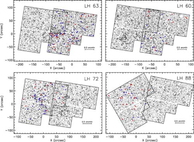
Figure 3.— Stellar charts of all stars detected with our WFPC2 photometry in both F555W and F814W filters in each of the observed Hii regions. Coordinates are given in seconds of arc from a reference point, which is selected to coincide with the center of WFPC2 Pointing 1 for every region. North is up and East is to the left of the charts. Bright candidate accreting PMS stars, identified from their H$\alpha$-excess (see § 4.1), and OB-type stars found with our photometry in shorter wavelengths (§ 4) are marked with red and blue symbols repsectively.

Figure is omitted due to size limitations.

Copy available upon request to the first author.

Figure 4.— Uncertainties of photometry as derived by HSTphot for all filters in the fields covered by Pointings 1 for each cluster.

Figure is omitted due to size limitations.

Copy available upon request to the first author.

Figure 5.— Completeness as it is evaluated by our artificial star experiments for the four broad-band filters in the regions covered by each Pointing 1.

We combined the photometric catalogs derived from the two pointings per cluster into one final catalog of stars detected in each targeted region. This process revealed 12 511 stars in LH 60, 11 785 in LH 63, 9 756 in LH 72 and 10 597 in LH 88 detected in both F555W and F814W filters. According to the methodology originally presented by Gouliermis, Brandner, & Henning (2006), and subsequently applied to various star-forming regions in both of the Magellanic Clouds (see, e.g., Sabbi et al., 2007; Gouliermis et al., 2007; Schmalzl et al., 2008; Cignoni et al., 2009; Vallenari, Chiosi, & Sordo, 2010), deep HST imaging in $V$- and $I$-equivalent wavelengths provides an efficient detection of PMS stellar populations from their positions in the corresponding CMD. Therefore, we assess the PMS stars in the observed regions from the complete photometric catalogs of stars detected in both the F555W and F814W filters in both pointings of each cluster. The corresponding stellar charts of the regions are shown in Fig. 3. In addition, since these filters provide the richest stellar samples, we also base the final multi-band photometric catalog of each cluster on the catalog of sources detected in both the F555W and F814W filters. A sample of this photometric catalog is shown in Table 3. Naturally, the photometry of stars identified in other pairs of filters are extremely useful and will be considered in subsequent analyses. For example the samples of stars detected in both F300W and F656N ($U$- and H$\alpha$-equivalent) certainly host PMS stars with accretion, which will be revealed from their $U$- and H$\alpha$-excess emission (see, e.g., Romaniello, Robberto, & Panagia, 2004; De Marchi, Panagia, & Romaniello, 2010); an analysis that we will apply in a forthcoming study. Moreover, multi-wavelength coverage of bright main-sequence (MS) stars is essential for the assessment of the interstellar reddening, which we perform later in this study.

2.3. Photometric accuracy and completeness

Photometric uncertainty and incompleteness are two factors that strongly depend on the targeted region. As a consequence both are higher in the frames centered on the Hii nebulae, due to higher stellar crowding and confusion by diffuse nebular emission. Fig. 4 shows typical uncertainties of photometry as a function of the magnitude for all filters, as obtained from our photometry on Pointings 1. As seen in Fig. 4 , photometric uncertainties behave similarly for each region in the F450W, F555W, and F814W filters. The F555W and F814W observations reach much fainter magnitudes accurately than those with the F300W and F450W filters. On average, the uncertainties of our photometry have $\epsilon<$ 0.1 mag for $m_{555}\ \raise-2.0pt\hbox{\hbox to0.0pt{\hbox{$\sim$}\hss}\raise 5.0pt\hbox{$<$}\ }$ 25.4 in all systems.

The completeness of our photometry was evaluated on the basis of artificial star experiments performed with the native artificial star function built into HSTphot for the creation of simulated images by distributing artificial stars of known positions and magnitudes. This utility allows the distribution of stars with similar colors and magnitudes as in the real CMD. It should be mentioned that due to the small image size of artificial stars generated within HSTphot the appearance of few bright saturated stars in each observed region leads to a somewhat underestimated completeness. The results of this process for the four broad-band filters used for Pointings 1 of each cluster are shown in Fig. 5. From these plots it can be seen that our photometry in Pointing 1 is more complete systematically for stars found in filters F555W and F814W. In most of the clusters, the photometric completeness in the F300W filter drops at brighter magnitudes, $m_{\rm 300}\simeq$ 22, while in F450W it is somewhat fainter. On average, we reach the limit of 50% completeness at $m_{\rm 555}\approx$ 26. Completeness in both F555W and F814W in WFPC2 Pointings 2 is slightly improved due to lower crowding and confusion.

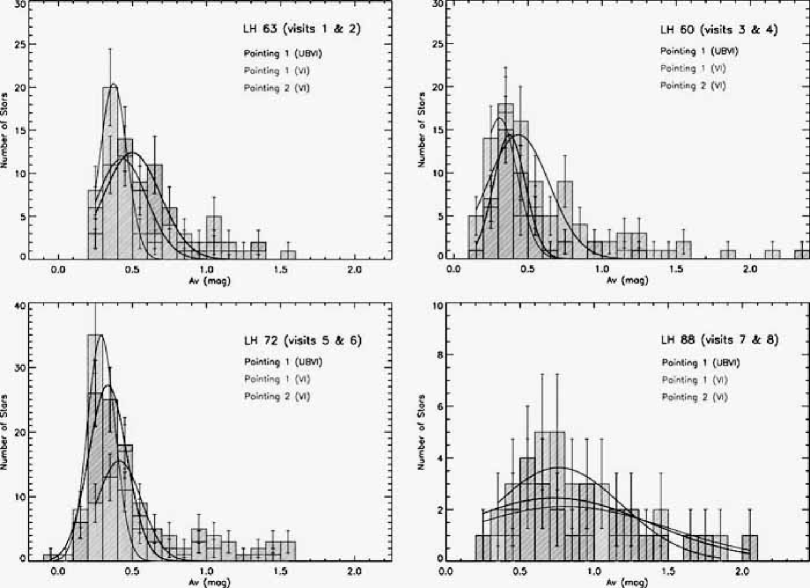
Figure 6.— Visual extinction distributions as derived from upper MS stars with $S/N>10$ with the use of observations in all four broad-band filters in Pointings 1, and in the $V$- and $I$-equivalents for Pointings 2 for every region. We evaluate extinction in Pointings 1 also with the use of only $V$- and $I$-equivalent filters for reasons of completion and comparison to those for Pointings 2. The best-fitting distributions to the histograms are overlaid. The derived average (peak) $A_{V}$ values and the corresponding 1$\sigma$ uncertainties are given in Table 4. [A color version of this figure will be available in the online journal.]

3. Interstellar Reddening

In this section we quantify the effect of interstellar extinction in the observed regions. We apply a statistical measurement of the visual extinction, $A_{V}$, in each observed region by constructing the distribution of the best-observed MS stars according to their extinction and obtaining its average value and 1$\sigma$ uncertainty. The calculation of $A_{V}$ toward the first WFPC2 pointing of each system is directly achieved from our observations in all four broad-band filters through comparison of data points in color-color diagrams to a model MS in the WFPC2 photometric system (Girardi et al., 2002). For this calculation we considered only stars with $S/N>10$ in all four bands, corresponding roughly to $m_{\rm 450}<19.5$ and $m_{\rm 300}-m_{\rm 450}<0$. However, the second WFPC2 pointing of each system is observed only in the bands F555W and F814W, and therefore we apply an additional independent $A_{V}$ measurement based on the comparison of the observed CMD positions of the upper MS stars to that expected according to the model MS. This measurement is applied for MS stars with $S/N>10$ in both bands, corresponding to $m_{\rm 555}<19.5$ and $m_{\rm 555}-m_{\rm 814}<0.5$.

The extinction law depends on the nature and composition of interstellar dust grains. Therefore the law will vary depending on environment such as Galactic star forming regions or for different galaxies like the Large and Small Magellanic Clouds (Gochermann & Schmidt-Kaler, 2002). Several investigations of the reddening law in the LMC show that the average LMC extinction curve does not differ from that of the Milky Way at wavelengths covered by $B$-, $V$- and $I$-equivalent filters (e.g., Koornneef & Code, 1981; Nandy et al., 1981; Fitzpatrick, 1986; Sauvage & Vigroux, 1991; Misselt et al., 1999), but with differences appearing in the $U$ band and for shorter wavelengths. Therefore, for the evaluation of extinction we assume the typical Galactic extinction law (e.g., Cardelli et al., 1989; Fitzpatrick & Massa, 1990), parameterized by a value of $R_{V}=A_{V}/E(B-V)=3.1$. Relative extinction was determined in the WFPC2 passbands from the analytical expression of stellar extinction of Fitzpatrick & Massa (1990).

Table 4Visual Extinction, $A_{V}$, toward the observed regions.

Region	WFPC2 Pointing 1		WFPC2 Pointing 2
	“$UBVI$”	“$VI$”	“$VI$”
LH 63	0.49 $\pm$ 0.19	0.37 $\pm$ 0.09	0.43 $\pm$ 0.17
LH 60	0.37 $\pm$ 0.10	0.31 $\pm$ 0.12	0.44 $\pm$ 0.21
LH 72	0.33 $\pm$ 0.13	0.29 $\pm$ 0.09	0.41 $\pm$ 0.15
LH 88	0.73 $\pm$ 0.64	0.81 $\pm$ 0.70	0.76 $\pm$ 0.42

Note. — The given $\pm$ values are the measured spreads, $\sigma$, in $A_{V}$, not the uncertainties in the measured values.

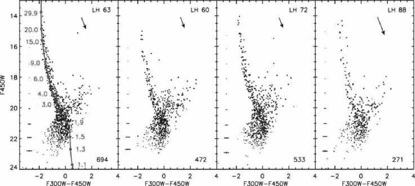
Figure 7.— The $UB$-equivalent CMDs of the stars detected with our photometry in both F300W and F450W filters in Pointings 1 of the observed regions. Arrows represent the maximum $A_{V}$ measurements given in Table 4. Typical photometric errors in both magnitudes and colors are shown on the left of each CMD. The numbers of stars with $\bar{\delta_{2}}\leq 0.1$ mag are given at the bottom-right of each diagram. The positions of these stars are indicated in the CMDs by thicker points. The ZAMS from the Girardi et al. (2002) grid of models is overlaid with indicative stellar mass values for MS stars. [A color version of this figure will be available in the online journal.]

Our results are shown in Fig. 6, where we plot the derived $A_{V}$ distributions for each Pointing of every observed region. The average extinction values per region and pointing are given with their 1$\sigma$ errors in Table 4. The fits applied to the histograms of Fig. 6 consider all stars within the selected $S/N$. It should be noted, however, that the CMD positions stars and most distant from the MS coincide with those of emission-line star-disk systems such as Be, B[e] stars (e.g., Wisniewski et al., 2007; Kraus, 2009), or of Herbig Ae/Be stars (e.g., Nishiyama et al., 2007; Clayton et al., 2010), which are expected in such star-forming regions. In addition, the appearance of binaries among MS stars will naturally lead to a small overestimation of the evaluated reddening. As a consequence, the derived values and errors of $A_{V}$ should be considered as the upper limits for the actual extinction. It is worth noting that, as shown from the values of Table 4, while in general Pointing 2 is less crowded and less affected by the Hii emission than Pointing 1, $A_{V}$ there is generally larger than in the latter. This is due to the higher concentration of dust on the rim of the Hii region, as is typical in such star-forming regions, which produces higher extinction on the periphery of the nebula.

In our subsequent analysis we will consider these upper values, rather than any lower average $A_{V}$ derived from the distributions after trimming the higher values bins. We will specifically use the maximum $A_{V}$ value, derived from the values of Table 4 as ${\langle A_{V}\rangle}_{\rm max}+\sigma_{\rm max}$ for each region. The reason for this approach is the fact that low-mass PMS stars in star-forming regions of the Magellanic Clouds occupy the fainter-redder part of the visual CMD, which can be strongly affected by reddening (see, e.g., Gouliermis et al., 2010). As a consequence faint low- and intermediate-mass MS stars may be confused for low-mass PMS stars due to reddening. Therefore, since it is important to apply a safe distinction between faint reddened MS and true PMS stars we quantify the maximum possible effect of visual extinction to the observed stellar samples in our qualitative distinction between PMS and reddened MS stars in the Hess diagrams and field-subtracted CMDs of the observed regions (see § 5). On the other hand, the quantitative selection of PMS stars according to their cross-section CMD distributions is not affected by the considerations of maximum reddening values, because these distributions in the CMDs of the less affected regions LH 60, LH 63 and LH 72 peak at colors redder than those of the expected most-reddened MS stars according to our reddening determinations (see § 6).

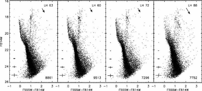
Figure 8.— The $VI$-equivalent CMDs of the stars detected with our photometry in both F555W and F814W filters in both Pointing 1 and 2 of each observed region. The numbers of stars with $\bar{\delta_{2}}\leq 0.1$ mag are given at the bottom-right of each diagram. The loci of the PMS stars cover the red sequence at $m_{\rm 814}$  $\sim$$>$  21, which is almost parallel to the MS. The intrinsic characteristics of these objects and possibly different ages among them are responsible for the spread of their CMD positions (see discussion in § 7. It is interesting to note that the CMD of LH 88 shows clear signs of extensive differential extinction in the system, apparent in the broad MS and elongated RC.

4. Color-Magnitude Diagrams

The $m_{\rm 300}-m_{\rm 450}$ versus $m_{\rm 450}$ ($UB$-equivalent) and $m_{\rm 555}-m_{\rm 814}$ versus $m_{\rm 814}$ ($VI$-equivalent) CMDs of the stars detected in the areas of the clusters are plotted in Figs. 7 and 8, respectively. Since only Pointing 1 was observed in the $U$- and $B$- equivalent wavebands, the corresponding CMDs show the stellar populations included only in this pointing of each cluster. On the other hand, both Pointing 1 and 2 were observed in the $V$- and $I$- equivalent wavelengths, and therefore the corresponding CMDs show the stellar populations covered by both pointings. Reddening vectors corresponding to the highest $A_{V}$ values derived in § 3, as they are given in Table 4, are also plotted in the CMDs. In order to select stars with the overall best photometry, we have used the average error in the two bands, $\bar{\delta_{2}}$, considered for every CMD set, given as

$$\bar{\delta_{2}}=\sqrt{\frac{\epsilon_{\rm 300}^{2}+\epsilon_{\rm 450}^{2}}{2}}~{}~{}{\rm or}~{}~{}\bar{\delta_{2}}=\sqrt{\frac{\epsilon_{\rm 555}^{2}+\epsilon_{\rm 814}^{2}}{2}}~{}~{},$$ (1)

respectively. The numbers of stars with $\bar{\delta_{2}}\leq 0.1$ mag in every stellar catalog are given at the bottom-right of each CMD.

In the CMDs of Figs. 7 and 8 it is shown that all observed regions are characterized by a variety of stellar species. The two sets of CMDs for every region, due to the selected filters and exposure times, track different types of stars, which nevertheless belong to the same system. In particular, the $UB$ CMDs of Fig. 7 indicate a sharp upper main-sequence (UMS) populated by the blue intermediate- and high-mass stars, which typically characterize embedded young LMC associations. According the the ZAMS model (plotted over the CMD for LH 63) all observed clusters host well-populated UMS mass functions with the most massive stars being O-type dwarfs with masses between 20 and 30 M_⊙. These stars and their relation to the observed clusters will be the subject of another subsequent analysis of the massive stellar content of these clusters. The OB stars revealed in the observed clusters from the $UB$-equivalent CMDs are shown with blue symbols in the stellar charts of Fig. 3.

In the present analysis we concentrate on the rich $VI$ CMDs of the clusters (Fig. 8). These CMDs are populated by a larger variety of stellar sources, covering the MS (faint and bright), the turn-off (TO), the red clump (RC), the red giant branch (RGB) and the PMS. These features represent two separate populations in the LMC, i.e., the evolved population of the general galaxy-field and the young and currently forming stellar populations of the clusters themselves. We describe each of these features in the following text. It should be noted that the observations presented in Fig. 8 are mainly focused on the faint stars, and therefore long exposures were performed in these filters. As a consequence, the UMS and the tip of the RGB are saturated and thus not shown. All four CMDs of Fig. 8 share all aforementioned features, and specifically apart from the UMS there is a pronounced TO at $m_{\rm 814}\simeq 21$ and a RGB with its RC located at $m_{\rm 814}\simeq 18$ and $m_{\rm 555}-m_{\rm 814}\simeq 1.0$. These two features are known to be typical of the LMC field, as we demonstrate later (in § 4.2; see also Fig. 10). Below the TO, moving to fainter magnitudes, the low main sequence (LMS) is the dominant feature of the CMDs. Previous HST imaging of other LMC star-forming regions has demonstrated that this population belongs entirely to the general LMC field and not the stellar systems (Gouliermis et al., 2007; Vallenari, Chiosi, & Sordo, 2010). On the other hand, the faint stellar membership of the young clusters at roughly the same brightness range with the LMS is located at redder colors in the CMDs, where a prominent broad sequence of PMS stars can be clearly seen in three of the observed regions. As we show later (§ 5) these stars belong only to the star-forming regions, and they are not related to the general LMC field.

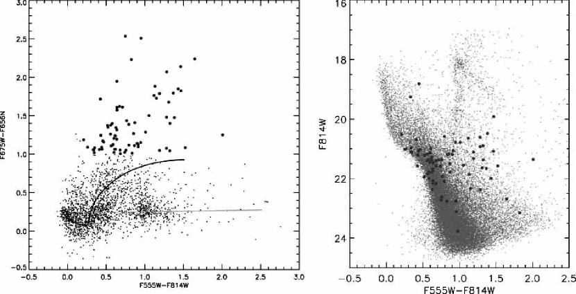
Figure 9.— Left: Diagnostic for stars with H$\alpha$ excess emission in the $R-{\rm H}\alpha$, $V-I$-equivalent color-color diagram. In this diagram the positions of normal stars without H$\alpha$ emission, i.e., field or weak-line T Tauri stars, are indicated by the blue line, and reddened field stars by the green. The group of stars with $R-{\rm H}\alpha\geq 1.0$ mag are mostly stars, which exhibit H$\alpha$ excess (plotted with red symbols). Right: The $VI$-equivalent CMD of the whole sample of observed stars in all four regions with H$\alpha$ excess emission candidate stars overlaid with red thick symbols. In this plot the CMD positions of bright PMS stars with H$\alpha$ excess can be readily identified, but the faint PMS populations are not covered due to the low sensitivity of the H$\alpha$ filter. The nature of the detected bright blue sources, as well as of cool objects with H$\alpha$ excess will be investigated in a subsequent study. [A color version of this figure will be available in the online journal.]

4.1. Stars with H$\alpha$ excess

PMS stars exhibit excess in their H$\alpha$ emission due to accretion. As a consequence the appearance of H$\alpha$ emission from stars in the clusters is a direct evidence of the existence of PMS stars in them. Nevertheless, if the age of the observed clusters is of the order of $\sim$ 3 Myr, H$\alpha$ emission stars should be very rare (see, e.g., Sung et al., 2004). In addition, the accretion rate of most PMS stars in the clusters may be very low, and therefore only few active stars would show H$\alpha$ emission, because only stars with equivalent widths $W({\rm H}{\alpha})>10$ Å can be detected photometrically with confidence (Sung et al., 2008). Sources with H$\alpha$ excess emission can be photometrically identified by the comparison of their H$\alpha$ and $R$-equivalent magnitudes (e.g., Sung et al., 1997). As our dataset lacks observations in the $R$-equivalent WFPC2 filter F675W, we determined a “synthetic” $m_{\rm 675}$ magnitude for every star derived by interpolation between data in the F555W and F814W bands, as described by De Marchi, Panagia, & Romaniello (2010). In total, 2 263 stars are detected in all three F555W, F814W and F656N bands with the best photometric quality in all four observed regions. We identify the H$\alpha$ excess stars in our sample by plotting the $m_{\rm 675}-m_{\rm 656}$ color index against the $m_{\rm 555}-m_{\rm 814}$ (Fig. 9, left). This diagnostic is equivalent to the use of the mean magnitude of $V$ and $I$ as a pseudocontinuum magnitude at H$\alpha$ (see, e.g., Sung et al., 2000; Sung & Bessell, 2004).

Considering that the reddening vector in Fig. 9 (left) is nearly parallel to the $m_{\rm 555}-m_{\rm 814}$ axis, the clump of stars around $m_{\rm 555}-m_{\rm 814}\sim 1.0$ and $m_{\rm 675}-m_{\rm 656}\sim 0.3$ represents highly reddened background stars. The green line in the figure indicates the meanline of these non-emission stars (e.g., Panagia et al., 2000; Sung & Bessell, 2004). In Fig. 9 (left) a large scatter in the $m_{\rm 675}-m_{\rm 656}$ index of normal stars, i.e., field stars or weak-line T Tauri stars, can also be seen. Taking into account the positions of these stars, indicated in the figure by the blue line, it is safe to select stars with $m_{\rm 675}-m_{\rm 656}$  $\sim$$>$  1.0 as candidate H$\alpha$ emission stars. As a consequence, for a first-order identification of the best candidates we apply tentatively the selection criterion requiring all H$\alpha$ emission stars to have $m_{\rm 675}-m_{\rm 656}\geq 1.0$ mag. Objects bluer than $m_{\rm 555}-m_{\rm 814}\simeq 0.2$ are probably Ae/Be stars (De Marchi, Panagia, & Romaniello, 2010), but considering the youthfulness of the clusters we should also expect a few massive PMS stars, i.e., Herbig Ae/Be stars. This selection revealed 78 sources, which appear in red in the $m_{\rm 675}-m_{\rm 656}$, $m_{\rm 555}-m_{\rm 814}$ diagram. These sources are marked with red symbols in the $VI$-equivalent CMD of all detected sources shown in Fig. 9, (right), and in the stellar maps shown in Fig. 3.

While our F656N observations provide direct evidence that the observed clusters host accreting PMS stars of intermediate and high mass, they are designed for the investigation of the bright stellar content of the clusters, and therefore they are not deep enough to cover the more populous low-mass PMS stellar content of the clusters. In fact, the aforementioned process identified PMS accreting candidates down to only $m_{\rm 814}\simeq 22$, much brighter than the vast majority of the low-mass PMS stars in the clusters. For the statistical identification of the latter we make use of the rich $VI$-equivalent CMDs, as described in the following sections. Nevertheless, a further thorough investigation of bright PMS stars with accretion, based on their H$\alpha$ equivalent widths, as well as their excess emission in the $U$-equivalent filter, and the analysis of the relation between H$\alpha$ strength and $U$-excess with accretion rate will be presented in a forthcoming paper.

4.2. Contribution of the general LMC Field

Naturally, the CMDs of Fig. 8 are ‘contaminated’ by the stellar populations of the general field of the LMC. In order to assess the field stellar population in the area of the observed regions, and evaluate this contamination, we retrieved from the HST Data Archive WFPC2 observations of empty regions of the LMC. Special care was taken to select observations, which are the most representative of the LMC field in the general vicinity of our LMC 4 target regions. In addition the fields should preferably have negligible differential extinction, and observational setup comparable to our own. Two WFPC2 pointings covered in the F555W and F814W bands matched best these criteria. The fields are observed within HST programs GO-10583 (PI: C. Stubbs) and GO-10903 (PI: A. Rest), both focused on the detection of LMC microlensing events in Cycles 14 and 15 respectively. Details on these observations are given in Table 1. Both our clusters and the general field were observed with almost identical setup of the instrument and exposure times, allowing a direct comparison between the $VI$ CMDs of the clusters and the local LMC field.

The CMDs of these LMC control-fields, shown in Fig. 10, outline the complete star formation history (SFH) of the galaxy, which has been well constrained by earlier studies with WFPC2 imaging. The results of these studies provide an accurate account of the evolutionary status of the stars we see in the CMDs of Fig. 10. According to these results, in general, the LMC disk is characterized by a continuous SFH for the last $\sim$ 10 to 15 Gyr (e.g., Smecker-Hane et al., 2002), with events of enhanced star formation that took place between 1 and 4 Gyr ago (Gallagher et al., 1996; Elson, Gilmore, & Santiago, 1997; Geha et al., 1998; Castro et al., 2001; Javiel, Santiago, & Kerber, 2005). These events are well recorded in the control-field CMDs of this study, as shown by the isochrones overlaid on the overall field CMD of Fig. 11 (left). These isochrones correspond to ages of roughly 0.8, 1.25, 2, 3, and 8 Gyr, proving this area to be somewhat younger than those described in the aforementioned studies, which are located outside LMC 4. A negligible visual extinction of $A_{V}=0.075$ mag, and the metallicity ($Z=0.008$) and distance of the LMC ($m-M=18.5$ mag) are applied to these models.

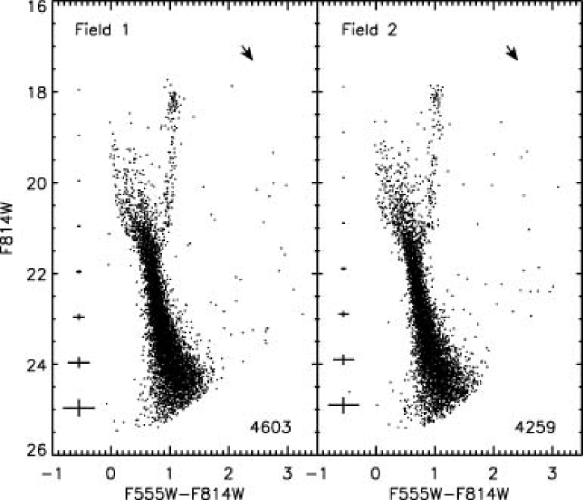
Figure 10.— The $VI$-equivalent CMDs of the stars detected with our photometry in both F555W and F814W filters in the two selected empty areas for the assessment of the general field of LMC in the region of LMC 4. These WFPC2 images were retrieved from the HST Data Archive (see § 2 and Table 1). The numbers of stars with $\bar{\delta_{2}}\leq 0.1$ mag are given at the bottom-right of each diagram.

5. Identification of PMS Stars in The Observed Regions

Low-mass PMS stars in LMC star-forming regions are known to cover the red-faint part of their $VI$-equivalent CMDs (see, e.g., Vallenari, Chiosi, & Sordo, 2010), and the regions observed here do not seem to be an exception. Indeed, a visual comparison between the CMDs of Fig. 8 and those of Fig. 10 verifies the existence of a broad sequence of PMS stars almost parallel to the LMS in the CMDs of the star-forming regions, which is completely missing from the control-field CMDs. In addition, the reddening range of early-type stars in the star-forming regions (Table 4), in comparison to that of the control-field ($A_{V}\simeq 0.075$) shows that reddening alone cannot explain the existence of very red population almost parallel to the LMS in the CMDs of the observed regions. In this part of the analysis we focus on methods for the identification of these PMS in the observed regions. In the cases of LH 60, LH 63, and LH 72 the appearance of PMS stars in the CMD is rather clear, but in the LH 88 region the higher reddening produces confusion in the unambiguous identification of PMS stars. The radical difference in the comprised populations between clusters and field is demonstrated more clearly in Fig. 11, where next to the overall control-field CMD with overlaid isochrones for evolved populations (left panel), the CMD of LH 60 is plotted with overlaid isochrones for PMS populations (right panel). These PMS models are constructed with the Frascati Raphson Newton Evolutionary Code (FRANEC, Chieffi & Straniero, 1989; Degl’Innocenti et al., 2008) for the metallicity of the LMC and the WFPC2 photometric system. They correspond to ages of 0.5, 1, 2, 3, 4, 5, 7.5, 10, 15, 20 and 30 Myr. This broad age-coverage demonstrates a well-documented problem in such observations, i.e., the wide spread of faint PMS stars, which does not necessarily correspond to any real age-spread among these stars, but it may well be the result of biases introduced by observational constrains, i.e., photometric accuracy and confusion, and the physical characteristics of these stars, such as variability, binarity and circumstellar extinction (see, e.g., Da Rio, Gouliermis, & Gennaro, 2010, for a detailed discussion).

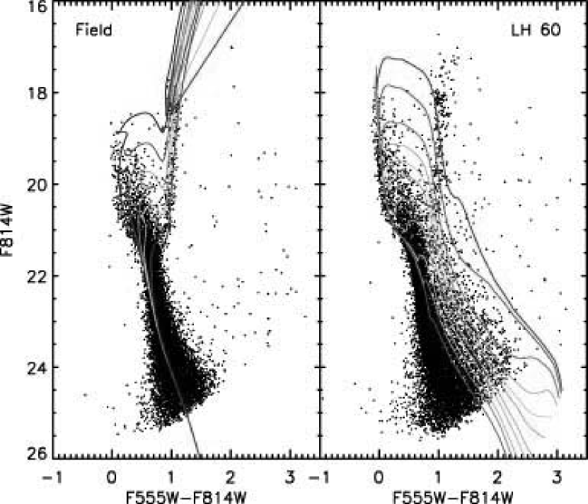
Figure 11.— Left: $VI$-equivalent CMD of the stars in the general LMC field at the vicinity of LMC 4 with isochrones for evolved stars overlaid. The models are taken from the Padova grid (Girardi et al., 2002) for the LMC metallicity ($Z=0.008$) and correspond to ages between roughly 1 and 10 Gyr in accordance with the established SFH of the galaxy. Right: $VI$-equivalent CMD of the stars in the observed region of LH 60 with isochrones for PMS stars overlaid. The models are constructed with the FRANEC code in the WFPC2 photometric system and the metallicity of the LMC (see § 5). [A color version of this figure will be available in the online journal.]

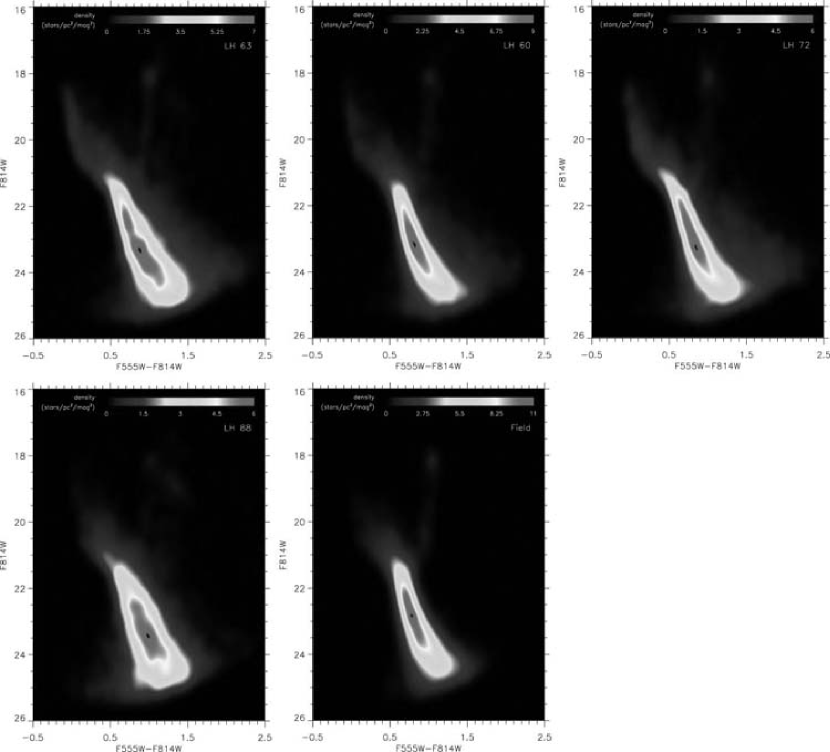
Figure 12.— Hess diagrams of the observed regions, and the general LMC field, constructed from their $VI$-equivalent CMDs. The diagrams are color-coded according to their stellar number densities indicated in the color bars. [A color version of this figure will be available in the online journal.]

The visual comparison of the CMDs of Fig. 11 outline three important aspects concerning the observed stellar populations: (1) The completely different evolutionary status of the field stars from that of the stellar content of the young clusters. (2) The great difficulty in distinguishing the evolved from the PMS populations at magnitudes brighter than $m_{\rm 814}\simeq 21.5$. (3) At fainter magnitudes the heavy contamination of the cluster CMD by the field populations, particularly in the LMS. Taking into account these aspects, it is important to establish an effective methodology for the determination of the true PMS stellar population of each observed young cluster/star-forming region. In this section we present such a scheme with the application of a qualitative approach based on the use of differential Hess Diagrams, and of a statistical field-subtraction technique based on the Monte Carlo method. Although these techniques provide a first distinction of the redder PMS from the bluer MS low-mass population of the clusters, they are indirect approaches in the determination of the true PMS populations. In particular, with each of these methods one can assess the field MS stellar contribution in the observed CMD in terms of stellar densities in the CMD, rather than on a star-by-star basis. Therefore, with these methods we cannot define the actual stars that should be considered as the most probable PMS stars, except for the reddest ones. As a consequence, we utilize these methods in order to demonstrate in a qualitative manner the existence of low-mass PMS stars in the observed regions. A quantitative statistical determination of the actual membership of each PMS candidate will take place in the next section with the construction of the stellar distributions of the observed stars along cross-sections of the faint part of each CMD. With this method a PMS membership probability is assigned to each red star, according to its CMD position with respect to the cross-sections stellar distributions across the CMD. In our analysis we consider only stars with the best photometric measurements, i.e., with $\bar{\delta_{2}}\leq 0.1$.

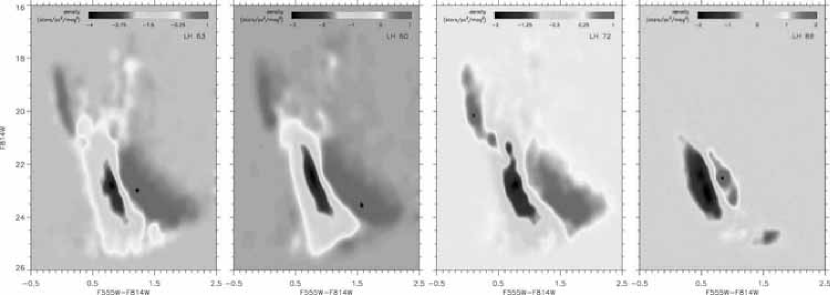
Figure 13.— Differential Hess diagrams of the observed regions derived by the subtraction of the Hess diagram of the general LMC field from those of the observed regions. [A color version of this figure will be available in the online journal.]

5.1. Differential Hess Diagrams

Fig. 12 shows the $VI$-equivalent Hess diagrams of the stars in the observed regions, as well as that of the overall general LMC field, i.e., the combined stellar content of the two control-fields. These diagrams are produced by binning the corresponding CMDs in 0.15 mag intervals in $m_{\rm 555}-m_{\rm 814}$ and 0.17 mag in $m_{\rm 814}$. The size of the binning is selected to be small enough to reveal the fine-structure in the stellar density, but also large enough to construct a realistic representation of the observed CMDs. Very small bin sizes would produce ‘noisy’ Hess diagrams, i.e., high numbers of small density peaks distributed throughout the diagrams, while large bin sizes would produce unrealistically thick Hess diagrams, which would smooth out any apparent effect of reddening or any true positional spread of stars in the CMD. The resulting two-dimensional distributions were smoothed by interpolation with a boxcar average. From the Hess diagrams of Fig. 12 it can be seen that the highest concentration of stars in all observed regions appears in the LMS. This part of the CMD is well-known to belong entirely to the general LMC field (§ 4.2). In the cases of LH 60, LH 63 and LH 72, at redder colors from the LMS and almost parallel to it, there is an apparent lower concentration of stars, which does not appear in the field. This feature corresponds to the faint PMS stars of the star-forming regions.

The differences between the observed systems and the field are more apparent in the residual or differential Hess diagrams. These are constructed with the subtraction of the field Hess diagram from those of the observed regions. Before this subtraction, we simulated the CMD of the observed regions by shifting fraction of stars in the CMD of the control field according to the reddening law, so that the morphology of the RGB in the simulated CMD is similar to that of the observed ones. Then we adjusted the number of RGB stars of the simulated field CMD to that of the target region. In addition, a broadening of the MS band due to photometric error was also simulated using a Monte Carlo technique. The resultant differential Hess diagrams are shown in Fig. 13. These diagrams for LH 60, LH 63 and LH 72 highlight the characteristic features of the $VI$-equivalent CMDs of typical LMC star-forming regions, i.e., a prominent UMS down to the intermediate-mass regime and a broad sequence of red faint PMS stars reaching the sub-solar mass-regime. In the differential Hess diagrams of Fig. 13 there are some residual stellar concentrations remaining in particular at the RC and some locations of the RGB. They are most likely due to the small number of stars in the corresponding grids, which do not allow a proper subtraction from the CMD of the observed regions. In addition, in the differential Hess diagrams of Fig. 13 there are no intermediate-mass PMS found in the Kelvin-Helmholtz contraction phase, located between the upper PMS and the MS, although there should be some such stars at least in LH 60, LH 63 and LH 72. A possible reason for this lack is the over subtraction of field stars on the TO. These points suggest that the differential Hess diagrams are subject to the normalization of the stellar numbers of the field, which nevertheless does not represent the real background field in the observed regions, as well as to the simulation process for the reproduction of this real field. Therefore, we rely on the Hess diagrams only for demonstrating the existence of a true PMS population of each region, and not for quantifying its members.

Considering the stellar distributions in the red-faint part of the CMDs of LH 60, LH 63 and LH 72, while the appearance of a sequence of stars in this part of the CMDs is quite obvious (see Figs 8, 12 and 13), one may argue that this part of the CMD is populated as a result of the effect of differential reddening on MS stars, rather than by actual PMS stars. However, if we consider the visual extinction measurements performed in § 3 and the maximum of the derived values given in Table 4, as well as the corresponding uncertainties, we cannot fully assign the observed red-faint stellar sequences to reddening of the MS alone. In particular, while the brightest part of the red-faint stellar sequence, at $m_{\rm 814}\simeq 21$ and $m_{\rm 555}-m_{\rm 814}\simeq 1$, may be partly explained by extinction, the colors covered by the faint part of the sequence are completely independent from a hypothetical differential reddening of the MS, as well as from the measured photometric errors at these magnitudes. This can be directly verified on the CMDs shown in Fig. 8 by considering the directions of the reddening vectors.

The analysis thus far shows that the PMS feature in the CMDs and Hess diagrams of the observed clusters appears to be quite distinct from a well-defined MS in the cases of LH 60, LH 63 and LH 72. On the other hand, the case of LH 88 seems to be quite different, because 1) we do not observe the same sequence of stars in the red faint part of the observed CMD and the corresponding Hess diagram of this region, and 2) the MS of LH 88 as seen in these diagrams is quite broader than those of the other regions and the field. This behavior can be explained by the higher extinction and its differential nature in the vicinity of LH 88. Indeed, there is a dense, thin residual sequence of stars to the red part of the LMS in the differential Hess diagram of LH 88 (Fig. 13), which does match the loose broad sequence of PMS stars seen in the other regions. This sequence could be misinterpreted as an ‘old’ PMS population, because the extinction measured for LH 88 (Table 4) can easily span its width. This stellar feature, thus, may include both reddened LMS stars and PMS stars. While we can not exclude the presence of PMS stars in LH 88, their loci should be well contaminated by reddened MS stars, and therefore their identification is not as straightforward as in the other regions.

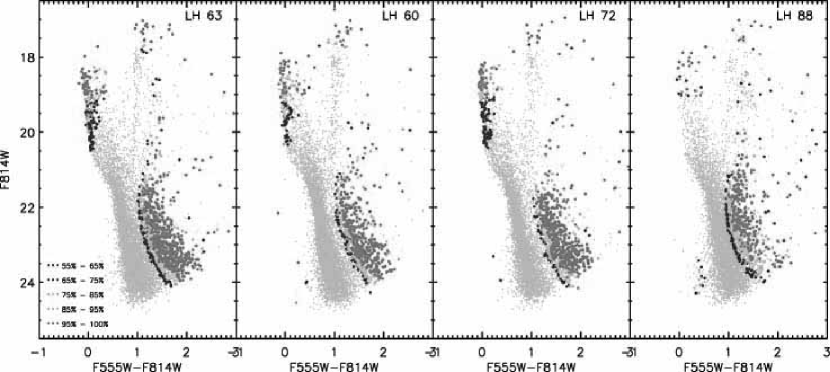
Figure 14.— Field-subtracted $VI$-equivalent CMDs for the observed star-forming regions. The remaining stellar members are color-coded according to their membership probabilities derived from the repeated application of our Monte Carlo method for the field decontamination (see § 5.2). [A color version of this figure will be available in the online journal.]

5.2. Statistical Identification of PMS stars: Subtraction of the field stars contamination

The stellar populations observed in the regions of the clusters are subject to strong contamination by the general LMC field. This contamination can be assessed statistically with the use of CMDs of the LMC field (Figs. 10, 11 left) and subtracted from the cluster CMDs with the application of a Monte Carlo method. For this method we consider a set of elliptical subregions around each star in the CMD of each cluster and the same set of subregions in the CMD of the LMC field. We then statistically subtract from the CMD of each system the corresponding number of randomly selected stars in the field CMD for each of these subregions. We perform 100 iterations of the Monte Carlo subtraction for each cluster, and we assign, thus, a percentage of membership probability, $p$, to every remaining star-member. The resultant field-subtracted CMDs of the clusters are shown in Fig. 14, overlaid on the originally observed CMDs (in grey). The stars remaining after the subtraction process are color-coded according to their assigned membership probability with $p\geq 55$%. In this figure it is shown that, as was the case in the Hess diagrams of the previous section, stars located in both the faint red and bright blue part of the CMDs are flagged as true members of the clusters. As it is observed also in the Hess diagrams of Fig. 13, after the field-subtraction there are few red evolved stars, which are falsely flagged as cluster members. These are residuals of the subtraction technique, which was not possible to be removed due to natural inconsistencies between the CMDs of the regions and that of the control-field.

The large majority of residual cluster-member stars with membership probability $p\geq 95$%, occupy the PMS part of the CMDs in Fig. 14. Naturally, this behavior characterizes the cases of LH 60, LH 63 and LH 72, where the PMS part of the CMD is fully populated by cluster-member stars down to the faintest detected magnitudes. On the other hand, in the case of LH 88, residual red stars with high membership probabilities correspond to somewhat brighter magnitudes and form a sequence connected to the residual field stars of the sub-giant branch and RC. Considering the high extinction of this region, the appearance of these red sources in a thin sequence almost attached to the red part of the LMS can be best explained by the effect of differential reddening on MS stars, rather than by these stars being PMS stars. The case for LH 63, which is also affected by - nonetheless lower - extinction, is not similar to that of LH 88, because the stars with high-membership probability populate completely the PMS part of the CMD as in the cases of LH 60 and LH 72. It is interesting to note that in the cases of these two clusters, which show the lowest extinction, there is a clear gap between the LMS and the PMS stars, making the distinction of the latter more straightforward.

Nevertheless, it should be noted that the results of the Monte Carlo subtraction technique are subject to its parameters. In particular the resulted ‘clean’ CMDs and the remaining stellar numbers depend on the size of the individual elliptical regions around each star considered for the random elimination of the field stars. Also this technique makes use of a general control-field rather than the actual field at the area of each observed region. Therefore, we treat the results of the Monte Carlo technique qualitatively and not quantitatively, as we did for the Hess diagrams. A quantitative analysis for the determination of the most probable PMS member-stars of each region is performed in the next section. Taking into account the results of this section, and in order to eliminate the appearance of reddened field stars in our PMS samples, in our subsequent analysis we concentrate on the fainter part of the CMDs with $m_{\rm 814}\ \raise-2.0pt\hbox{\hbox to0.0pt{\hbox{$\sim$}\hss}\raise 5.0pt\hbox{$>$}\ }21$.

6. Membership determination of PMS stars in the observed regions

In this section we perform a statistical determination of the membership of the PMS stars in each observed star-forming region by constructing the stellar distributions along cross-sections of the observed CMDs. Since, as discussed above, at magnitudes brighter than $m_{814}\sim 21$ there is a confusion between PMS and evolved stars, we limit our treatment to the fainter part of each CMD. We consider again only the stars found with photometric uncertainties $\bar{\delta_{2}}\leq 0.1$.

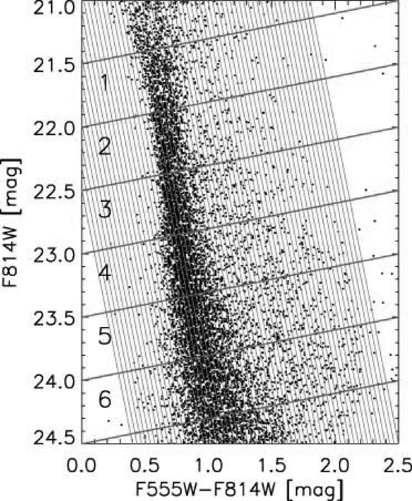
Figure 15.— Example of the stellar counting process for the construction of the distribution of stars along cross-sections through the observed $VI$-equivalent CMD of LH 60. The six selected cross-sections perpendicular to the MS and the PMS locus are indicated by the red lines, covering the whole faint part of the observed magnitude range. The strips selected for the binning of the stars along the cross-sections, and the construction of the corresponding stellar distributions are indicated by the blue lines, almost parallel to the MS. [A color version of this figure will be available in the online journal.]

6.1. Stellar distributions along cross-sections of the CMD

A more quantitative analysis of the observed PMS populations is achieved by counting the number of stars as a function of their ($m_{555}-m_{814}$) colors along a series of CMD cross-sections perpendicular to the PMS locus. This method is previously established for the identification of PMS stars in $VI$ CMDs of Galactic star-forming regions (see, e.g., Sherry, Walter, & Wolk, 2004). An example of the counting process for the construction of the stellar distributions along six cross-sections, selected to cover the magnitude range of interest, i.e., 21.5  $\sim$$<$  $m_{814}$  $\sim$$<$ 24.5, is shown in Fig. 15 for LH 60. The cross-sections are indicated by the red lines with their numbers marked. Stars are binned in strips perpendicular to the cross-sections and thus almost parallel to the MS. These strips, which are also almost parallel to typical PMS isochrones derived from PMS evolutionary models (e.g., Palla & Stahler, 1999; Siess, Dufour, & Forestini, 2000), are indicated in Fig. 15 by the blue lines.

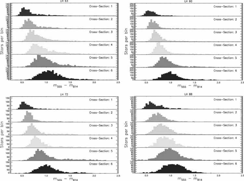
Figure 16.— Stellar distributions along selected cross-sections of the CMDs of the observed regions. Since we are interested in the faint PMS populations of the clusters we constrain our analysis to six cross-sections through the CMD, covering the magnitude range 21.5  $\sim$$<$  $m_{814}$  $\sim$$<$ 24.5. Stars are counted in bins 0.035 mag wide and the derived distributions are plotted with respect to the corresponding average color ($m_{\rm 555}-m_{\rm 814}$) of each bin. Different colors are used for the distributions of different cross-sections. Stellar numbers are corrected for incompleteness. These plots reveal the PMS populations of the observed clusters as a secondary distribution red-ward from that peaked on the field MS stars. [A color version of this figure will be available in the online journal.]

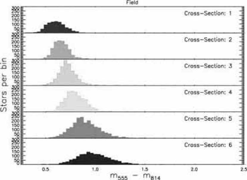
Figure 17.— Same as Fig. 16 for the total population of the general LMC field. [A color version of this figure will be available in the online journal.]

The constructed stellar distributions are shown in Fig. 16. Stellar numbers are corrected for incompleteness according to our completeness measurements described in § 2.3. Since the distribution of stars and nebula is not uniform across each observed field, confusion may also vary across each region, being higher at the most crowded regions. As a consequence, photometric completeness not only is a function of the observed magnitudes but also depends on the position of each star across the field. Therefore, we corrected the numbers of stars per bin in every strip on a single-star basis according to the magnitude and position of each star in the observed field. In Fig. 16 it can be seen that the distribution of stars for each cross-section is peaked on the field MS, which comprises the large majority of the observed stars in each target. Our aim is to identify the stellar distributions that correspond to the redder PMS population of the star-forming regions. Indeed, as it can be seen for the regions LH 60, LH 63 and LH 72, their stellar distributions are not symmetrically peaked on the MS and are clearly extended to the red, especially for cross-sections with $m_{814}$  $\sim$$<$ 24.0. It should be noted that, the red-ward asymmetry of their stellar distributions cannot be attributed to reddening alone based on our visual extinction estimates.

For comparison to these distributions we show in Fig. 17 the corresponding stellar distributions derived from the CMD of the control fields (Figs. 10, 11). From the distributions of Fig. 17 it is shown that field stars, in contrast to those of the star-forming regions, are distributed symmetrically around the MS. Again, the case of LH 88 fits more this behavior, rather than that of the other three regions of our sample. The stellar distributions in LH 88, shown in Fig. 16, appear symmetrically peaked on the MS, as in the case of the LMC field, but much broader than the general field, most probably due to the high extinction that characterizes this region. Under these circumstances, even if there are PMS stars in LH 88, we cannot accurately assess their numbers. In all of the discussed distributions, the wider spread of stars for cross-sections corresponding to fainter magnitudes can be naturally attributed to the larger photometric uncertainties.

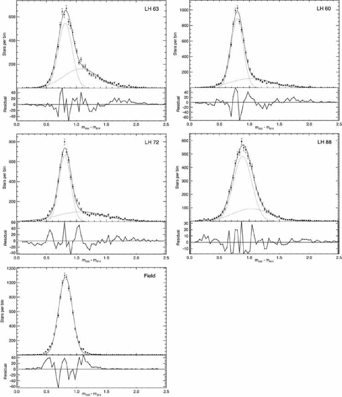
Figure 18.— Cumulative stellar distributions along all considered cross-sections of the CMDs for the magnitude range 21.5  $\sim$$<$  $m_{814}$  $\sim$$<$ 24.5. Stars are counted in bins 0.035 mag wide and their numbers are corrected for incompleteness. The distributions are plotted with respect to the average color ($m_{\rm 555}-m_{\rm 814}$) of each strip (bin). The best-fit double Gaussian function is overlaid with a red line. Each component of this function is also drawn with orange lines. Errors represent Poisson statistics. Residuals are plotted below each fit, demonstrating the goodness-of-fit. [A color version of this figure will be available in the online journal.]

Considering the above, the distribution of stars along cross-sections through the CMDs of the star-forming regions can be well represented by the sum of two distributions; one for the field MS stars and one of the native PMS stars of the regions. For demonstration we apply such a fit to the cumulative stellar distribution for each region and the field. These distributions are constructed by counting the stars in the selected strips parallel to the MS for the whole considered magnitude range, i.e., in all six selected cross-sections, as they are shown in Fig. 15. In this manner, the peak of the distribution will keep following the original peaks on the MS of the individual cross-sections. On the other hand, since the counting bins (strips) are not vertical to the color axis, each bin in the cumulative distribution does not correspond to a single color value. Therefore, we assign to each bin the average color index, which roughly corresponds to that of the average magnitude of $m_{814}\simeq 23$.

We fit the number of stars per bin of the cumulative distributions to a double Gaussian function of the form

$$y=\displaystyle\sum\limits_{i=1}^{2}N_{i}e^{-0.5((x-\mu_{i})/\sigma_{i})^{2}}.$$ (2)

The first term describes the distribution of field MS stars and the second that of the PMS stars. We use a least-squares multiple Gaussian fit performed by the interactive IDL routine xgaussfit (by Don Lindler) to solve for six parameters, $N_{i}$, $\mu_{i}$, and $\sigma_{i}$, where $i=1$ is for the field and $i=2$ for the PMS stars. The constructed cumulative stellar distributions across the CMDs of the observed regions and the LMC field are shown in Fig. 18. The best-fitted Gaussian distributions derived from our fitting process are also drawn; the total fit is indicated with a red line, while each of the two Gaussian components is drawn with an orange line. The corresponding residuals of the fits are accordingly drawn in order to show the goodness of each fit.

From the plots of this figure for LH 60, LH 63 and LH 72 one can see that the red component of the stellar distributions along the cross-sections of the CMDs is indeed important and successfully represented by a Gaussian distribution. In the case of LH 88 the contribution of the red component to the stellar distribution turns out – as expected – not to be significant, as can be seen by the fits. The cumulative distribution of stars in the field CMD is shown also in Fig. 18 for comparison. Naturally, only a single-Gaussian fit could be applied to this distribution. The coefficients of the fits shown in Fig. 18 are given in Table 5. The values of this table show the remarkable coincidence of the primary peak in the distributions of the star-forming regions with the Gaussian function representing the general field. This coincidence, which is more prominent in LH 60, LH 63 and LH 72, provides additional evidence of the field origin of the MS population observed in the CMDs of these star-forming regions.

Table 5Coefficients of the best-fitting double Gaussian function to the cumulative distributions of faint stars across the CMDs.

	Gaussian component 1			Gaussian component 2
Region	$N_{1}$	$\mu_{1}$	FWHM1	$N_{2}$	$\mu_{2}$	FWHM2
LH 63	547	0.82	0.27	162	1.08	0.68
LH 60	888	0.80	0.24	118	1.03	0.78
LH 72	663	0.81	0.23	96	1.08	0.94
LH 88	483	0.89	0.36	93	1.03	0.71
Field	1071	0.82	0.27

This fitting process is performed for the stellar distributions along each of the selected cross-sections for each observed CMD. The distribution of the field stars per se is not interesting, but it is crucial because the number of PMS stars depends upon the extrapolation of the field star distribution through the PMS locus. The total number of PMS stars along a cross-section is determined by the normalization of the Gaussian fit to the PMS distribution, $N_{2,j}$ (where $j=1,...,6$ is the cross-section number), and by $\sigma_{2,j}$, which defines the width of the Gaussian. The full width at half maximum (FWHM) of the PMS population is 2${\sigma_{2,j}}{\sqrt{2ln(2)}}$. The $\mu_{2,j}$ parameter is the color $m_{555}-m_{814}$ of the peak of the PMS distribution along a cross-section. Since each cross-section is a predefined line across the CMD, $\mu_{2,j}$ specifies the magnitude that corresponds to the peak of the PMS distribution. The coefficients of the best-fit second Gaussian component, representative of the PMS population, for each cross-section are given in Table 6.

We fit the field and PMS distributions jointly, and we derive the total number of PMS stars from the second Gaussian component of each fit by assigning a membership probability to each star. This probability is determined by the ratio of the second Gaussian component of the fit to the total fit along each cross-section through the CMD, i.e., the sum of both Gaussian components of the fit. Membership probabilities calculated in this manner vary from 0% to the blue of the PMS locus to $>$90% near the peak of the PMS distribution and for redder colors in all cross-sections. We thus derive 1 815 stars in LH 63, 1 230 in LH 60, 1 223 in LH 72 and only 314 in LH 88 with probabilities of cluster membership $p\geq 95\%$. These numbers are completeness corrected.

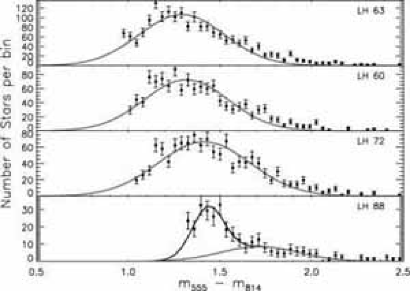
Figure 19.— Cumulative stellar distributions across the CMDs of the observed regions for the stars found with membership probability $p\geq 95\%$. The PMS populations of LH 60, LH 63 and LH 72 demonstrate an extraordinary similarity, which possibly indicates their common characteristics. On the other hand the distribution for LH 88 demonstrates the difficulty in disentangling the true stellar population of the region, since stars with high membership probability seem to represent reddened MS stars and not PMS stars, which are possibly represented by the second (faint) peak. [A color version of this figure will be available in the online journal.]

Table 6Coefficients of the best-fitting Gaussian component 2 of the fits to each of the individual cross-sections distributions of faint stars across the CMDs.

	LH 63			LH 60			LH 72			LH 88
Cross-section	$N_{2}$	$\mu_{2}$	FWHM2	$N_{2}$	$\mu_{2}$	FWHM2	$N_{2}$	$\mu_{2}$	FWHM2	$N_{2}$	$\mu_{2}$	FWHM2
1	17	0.79	0.49	11	0.85	0.45	9	1.00	0.58	8	1.17	0.43
2	21	0.93	0.51	14	0.90	0.45	14	0.92	0.66	14	0.93	0.45
3	53	0.86	0.41	31	0.89	0.42	14	1.09	0.76	24	0.98	0.49
4	37	1.09	0.60	24	1.07	0.70	18	1.17	0.86	18	1.14	0.53
5	31	1.25	0.76	32	1.13	0.73	20	1.32	1.05	20	1.09	0.81
6	14	1.45	0.73	16	1.30	0.89	13	1.46	0.74	6	1.61	0.14

This particular statistical technique for the determination of cluster membership probabilities of PMS stars is quite self-consistent, because it makes use of the LMC field as it is observed within each region and not of a generic remote field as in the case of the Monte Carlo field subtraction presented in § 5.2. Moreover, the use of the cross-sections distributions for the determination of the most probable PMS stars is independent of the reddening measurements in each region. It is interesting to note that this technique returned two times more PMS member candidates (with $p\geq 95\%$) than the Monte Carlo field subtraction, except in the case of LH 88, where the derived numbers are comparable. The reason for this difference lies on the elimination by the Monte Carlo technique of the red wing of the LMS from the CMDs of the star-forming regions as field candidates. Since this technique is based on the iterative random subtraction of candidate field contaminants within individual CMD-regions around each observed star, the subtraction of different stars in each repetition results in low membership probabilities for all stars in CMD-regions where field stars are expected to be located. On the other hand, the cross-sections technique, being dependent solely on the actual CMD positions of the observed stars and their distributions, returns a purely probabilistic membership determination for each star, independent of the appearance of field stars or not in its surrounding CMD-region.

7. Discussion

In Fig. 19 we show the cumulative distributions along the CMD only for the PMS stars of each region, i.e., for those stars found with a membership probability $p\geq$  95%. These distributions are constructed as those for all observed stars by counting them in strips (bins) parallel to the MS, as described in § 6.1. As for those distributions, the color index per bin is the average, corresponding to that at magnitude $m_{814}\simeq 23$. The distributions of Fig. 19 show an extraordinary similarity for the cases of LH 60, LH 63 and LH 72. Indeed, the fitting coefficients of the best-fitted Gaussian functions (drawn in red) are almost identical. Specifically, the peaks $\mu$ of the fitting functions are equal to 1.32, 1.29 and 1.41, and the corresponding widths $\sigma$ are 0.23, 0.23 and 0.25 for LH 60, LH 63 and LH 72 respectively. The case of LH 88 is again an outlier and it is shown only for completeness. The CMD distribution of the ‘best candidate’ stellar members for LH 88 is not represented by a single but by two Gaussians, with the first component of the fit (drawn in blue) being very narrow. This clearly suggests that the stars flagged in the previous section as best candidates for members of the star-forming region, and especially those at bluer colors, are in fact misidentified reddened MS stars. The smaller red Gaussian component may represent traces of the PMS population of the system, which is contaminated by reddened evolved stars, but this result cannot be conclusive.

The CMD distributions of the stellar members of LH 60, LH 63 and LH 72 show that these PMS stars cover a broad area of the CMDs of these regions. Indeed, the loci of PMS stars in the CMDs of Milky Way star-forming regions often show a widening, which could be evidence for age-spread (Briceño et al., 2007). This is also observed in young clusters and associations of both the Magellanic Clouds imaged with HST (see e.g., Gouliermis et al., 2010), and our results so far show that the regions investigated here are not exceptions. However, simulations performed previously by us have shown that characteristics of PMS stars, such as variability, binarity and circumstellar extinction can cause considerable scatter of the positions of the PMS stars in the CMD, giving false evidence of an age-spread within the systems (Hennekemper et al., 2008; Da Rio, Gouliermis, & Gennaro, 2010). Consequently we cannot attribute the observed CMD broadening of PMS stars solely to age-spread.

Nevertheless, the distributions of Fig. 19 convey valuable information about the most probable ages of the systems and their indicative age-spreads. Taking the peaks of the cumulative distributions at ‘face value’ one can conclude that LH 63 should be somewhat older than LH 60 and LH 72, because it corresponds to a bluer color, and thus to an older age. However, considering the PMS stellar distributions in the individual cross-sections across the CMDs for all three regions, they are all consistent with each other, peaking at colors along isochrones of ages between $\sim$ 3 and 5 Myr, with the cases of LH 60 and LH 72 showing to be somewhat closer to the $\sim$ 3 Myr isochrone. As far as the widths of the PMS distributions are concerned, they overlap with each other so well so that one cannot conclude any specific age difference among the three clusters. The derived age span of $\sim$ 3 to 5 Myr is in excellent agreement with the age of the star-forming region LH 95, located at the north-western edge of the super-giant shell LMC 4, derived by a self-consistent age determination technique developed by us (Da Rio, Gouliermis, & Gennaro, 2010). In a subsequent study we will apply this technique to the data presented here, in order to constrain further the ages of the systems. It is worth noting that taking also the widths of the distributions at ‘face value’, they correspond to a significant spread between 2 and 10 Myr. This result, however, is to be tested in our forthcoming study.

Another factor to be considered as responsible for the CMD broadening of PMS stars is differential reddening. However, while the PMS stars are expected to be somewhat dislocated due to reddening, our measurements of visual extinction, discussed in § 3, show that differential reddening cannot either be fully responsible for the scattering of PMS stars in the CMDs of these three regions. Our measurements show that $A_{V}$ in all investigated systems, except of LH 88, is quite low with a small variation with a maximum of $A_{V}\simeq 0.68$ mag (for LH 63), corresponding roughly to color excess of $E({\rm F555W}-{\rm F814W})\simeq 0.27$ mag, much smaller than the FWHM of the observed PMS broadening. On the other hand, LH 88 suffers from the highest extinction, with a maximum of $A_{V}\simeq 1.5$ mag, which appears to be adequate to account for the observed CMD spread of stars.

In conclusion, for the regions LH 60, LH 63 and LH 72, the cross-sections distributions of the PMS stars with $m_{\rm 814}$   $\sim$$>$  21.5 seem to be quite similar to each other in respect to their total numbers of stars, to their peaks and widths, as well as to the average color index at which the peak in stellar numbers appears. These extraordinary similarities clearly imply that the PMS stars found in three different young clusters, embedded in star-forming regions along the periphery of LMC 4, have possibly similar characteristics, and probably share a common star formation history.

8. Summary and Concluding Remarks

In this paper we present the first part of our investigation of PMS stellar populations in the LMC. Our targets of interest are four star-forming regions, LH 60, LH 63, LH 72 and LH 88, located along the rim of the super-giant shell LMC 4. We present the reduction of the multi-wavelength images taken with HST WFPC2 within our program GO-11547 (PI: D. Gouliermis), and our photometric analysis. We determine the accuracy and completeness of our photometry, and we measure the visual extinction towards the regions. We identify the stellar populations comprised in the observed fields in terms of the constructed CMDs. We evaluate the contribution by the field stellar populations with the use of archival WFPC2 images of the local LMC field. We make use of our rich photometric catalogs in the F555W and F814W ($V$- and $I$-equivalent) filters to assess the stellar content of the clusters embedded in the observed regions.

We demonstrate that the true stellar content of the star-forming regions comprises both bright young stars observed at the UMS of their CMDs and faint stars still in the PMS phase of their evolution. An outlier from this general behavior is the region of LH 88, the high extinction of which does not allow a clear identification of its true populations. The identification of the PMS stars in the observed clusters is performed through the assessment of the contamination of the observed populations by the stellar content of the LMC field. This is achieved qualitatively by the construction of the differential Hess diagrams of the observed regions (§ 5.1), and the derivation of the “clean” CMDs of the clusters after the statistical subtraction of the contaminant field population from the observed CMDs (§ 5.2).

The probabilistic identification of the PMS stars in the observed regions is further performed, in a quantitative manner, by the distributions of the stars along cross-sections of the observed CMDs (§ 6). We particularly focus on the faint PMS populations of the clusters, and we constrain our analysis to the fainter part of the CMDs with $m_{\rm 814}\ \raise-2.0pt\hbox{\hbox to0.0pt{\hbox{$\sim$}\hss}\raise 5.0pt\hbox{$>$}\ }21.5$, which is less contaminated by evolved field populations. We construct the number distributions of the stars across each observed CMD along six selected magnitude ranges and we fit these distributions with a two Gaussian components. The first component represents the MS field stars observed in each region, while the second corresponds to the PMS member stars of the region. For each star we assign a membership probability, $p$, derived from the ratio of the second fitted Gaussian to the sum of the two components along each cross-section. We isolate the stars with $p\geq$ 95%, as the best candidates of being members of the star-forming regions. All these candidates are PMS stars. The CMD distributions of these stars show an extraordinary similarity to one another for the regions LH 60, LH 63 and LH 72, suggesting similar characteristics. Considering that the peaks of these distributions represent the most probable ages of the regions, their similarity also suggests that all three regions may share a common recent star formation history. This result is quite important, since these regions are located at different parts of the boundaries of the super-giant shell LMC 4, and therefore our findings suggest that star formation around the shell may have occurred almost simultaneously. Nevertheless, these distributions show a definite widening of the loci of faint PMS stars in the observed $VI$-equivalent CMDs, which should be further investigated.

The spread of PMS stars along the color axis in the CMDs of star-forming regions in the Magellanic Clouds is a well-documented phenomenon, which demonstrates that the particular location of a PMS star in the CMD is a very complex function of its intrinsic properties (see, e.g., Gouliermis et al., 2010). Low-mass PMS stars in such regions, being the counterpart of Galactic T Tauri stars, suffer from rotational variability, non-periodic variability due to accretion, circumstellar extinction, and binarity. These characteristics dislocate the stars from their original positions in the CMD in an unpredictable manner, which may be misinterpreted as an age-spread within the host stellar system. The only accurate approach to quantify this effect and to confirm or refute the spread in ages is through detailed simulations of synthetic CMDs and their comparison to the observed ones. We are currently undertaking such an investigation with the accurate statistical determination of the masses and ages of the identified PMS stars through two self-consistent techniques established by us (see Da Rio, Gouliermis, & Henning, 2009; Da Rio, Gouliermis, & Gennaro, 2010). Our subsequent investigation of the observed star-forming regions will include the multi-wavelength characterization of the bright stellar content of the clusters (see, e.g., Romaniello et al., 2002), the determination of circumstellar accretion of bright PMS stars through their $U$- and H$\alpha$-excess emission (e.g., De Marchi, Panagia, & Romaniello, 2010), and the identification of embedded massive candidate young stellar objects and ultra-compact Hii regions via the synergy of our observations with those in longer wavelengths (e.g., Gruendl & Chu, 2009).

References

- Bica et al. (1999) Bica, E. L. D., Schmitt, H. R., Dutra, C. M., & Oliveira, H. L. 1999, AJ, 117, 238
- Briceño et al. (2007) Briceño, C., Preibisch, T., Sherry, W. H., Mamajek, E. A., Mathieu, R. D., Walter, F. M., & Zinnecker, H. 2007, Protostars and Planets V, 345
- Cardelli et al. (1989) Cardelli J.A., Clayton G.C., Mathis J.S., 1989, ApJ, 345, 245
- Castro et al. (2001) Castro, R., Santiago, B. X., Gilmore, G. F., Beaulieu, S., & Johnson, R. A. 2001, MNRAS, 326, 333
- Chieffi & Straniero (1989) Chieffi, A., & Straniero, O. 1989, ApJS, 71, 47
- Chu (2009) Chu, Y.-H. 2009, IAU Symposium, 256, The Magellanic System: Stars, Gas, and Galaxies, ed. J. Th. van Loon & J. M. Oliveira (Cambridge: Cambridge Univ. Press), 166
- Cignoni et al. (2009) Cignoni, M., et al. 2009, AJ, 137, 3668
- Clayton et al. (2010) Clayton, G. C., et al. 2010, ApJ, 722, 1131
- Da Rio, Gouliermis, & Henning (2009) Da Rio, N., Gouliermis, D. A., & Henning, T. 2009, ApJ, 696, 528
- Da Rio, Gouliermis, & Gennaro (2010) Da Rio, N., Gouliermis, D. A., & Gennaro, M. 2010, ApJ, 723, 166
- De Marchi, Panagia, & Romaniello (2010) De Marchi, G., Panagia, N., & Romaniello, M. 2010, ApJ, 715, 1
- Degl’Innocenti et al. (2008) Degl’Innocenti, S., Prada Moroni, P. G., Marconi, M., & Ruoppo, A. 2008, Ap&SS, 316, 25
- Davies, Elliott, & Meaburn (1976) Davies, R. D., Elliott, K. H., & Meaburn, J. 1976, MmRAS, 81, 89
- Dolphin (2000) Dolphin, A. E. 2000, PASP, 112, 1383
- Dolphin (2002) Dolphin, A. E. 2002, The 2002 HST Calibration Workshop : Hubble after the Installation of the ACS and the NICMOS Cooling System, 301
- Dopita, Mathewson, & Ford (1985) Dopita, M. A., Mathewson, D. S., & Ford, V. L. 1985, ApJ, 297, 599
- Elson, Gilmore, & Santiago (1997) Elson, R. A. W., Gilmore, G. F., & Santiago, B. X. 1997, MNRAS, 289, 157
- Fitzpatrick (1986) Fitzpatrick, E. L. 1986, AJ, 92, 1068
- Fitzpatrick & Massa (1990) Fitzpatrick, E. L., & Massa, D. 1990, ApJS, 72, 163
- Gallagher et al. (1996) Gallagher, J. S., et al. 1996, ApJ, 466, 732
- Geha et al. (1998) Geha, M. C., et al. 1998, AJ, 115, 1045
- Girardi et al. (2002) Girardi, L., Bertelli, G., Bressan, A., Chiosi, C., Groenewegen, M. A. T., Marigo, P., Salasnich, B., & Weiss, A. 2002, A&A, 391, 195
- Gochermann & Schmidt-Kaler (2002) Gochermann, J., & Schmidt-Kaler, T. 2002, A&A, 391, 187
- Gouliermis, Brandner, & Henning (2006) Gouliermis, D., Brandner, W., & Henning, T. 2006, ApJ, 636, L133
- Gouliermis et al. (2007) Gouliermis, D. A., Henning, T., Brandner, W., Dolphin, A. E., Rosa, M., & Brandl, B. 2007, ApJ, 665, L27
- Gouliermis et al. (2010) Gouliermis, D. A., et al. 2010, The Impact of HST on European Astronomy, 71
- Gruendl & Chu (2009) Gruendl, R. A., & Chu, Y.-H. 2009, ApJS, 184, 172
- Henize (1956) Henize, K. G. 1956, ApJS, 2, 315
- Hennekemper et al. (2008) Hennekemper, E., Gouliermis, D. A., Henning, T., Brandner, W., & Dolphin, A. E. 2008, ApJ, 672, 914
- Hill, Madore, & Freedman (1994) Hill, R. J., Madore, B. F., & Freedman, W. L. 1994, ApJS, 91, 583
- Javiel, Santiago, & Kerber (2005) Javiel, S. C., Santiago, B. X., & Kerber, L. O. 2005, A&A, 431, 73
- Karttunen et al. (2007) Karttunen, H., et al., 2007, Fundamental Astronomy, 5th Edition (Springer Berlin Heidelberg New York)
- Koornneef & Code (1981) Koornneef, J., & Code, A. D. 1981, ApJ, 247, 860
- Kraus (2009) Kraus, M. 2009, A&A, 494, 253
- Kroupa (2002) Kroupa, P. 2002, Science, 295, 82
- Lucke & Hodge (1970) Lucke, P. B., & Hodge, P. W. 1970, AJ, 75, 171
- Meaburn (1980) Meaburn, J. 1980, MNRAS, 192, 365
- Misselt et al. (1999) Misselt, K. A., Clayton, G. C., & Gordon, K. D. 1999, ApJ, 515, 128
- Nandy et al. (1981) Nandy, K., Morgan, D. H., Willis, A. J., Wilson, R., & Gondhalekar, P. M. 1981, MNRAS, 196, 955
- Nishiyama et al. (2007) Nishiyama, S., et al. 2007, ApJ, 658, 358
- Olsen, Kim, & Buss (2001) Olsen, K. A. G., Kim, S., & Buss, J. F. 2001, AJ, 121, 3075
- Palla & Stahler (1999) Palla, F., & Stahler, S. W. 1999, ApJ, 525, 772
- Panagia et al. (2000) Panagia, N., Romaniello, M., Scuderi, S., & Kirshner, R. P. 2000, ApJ, 539, 197
- Romaniello et al. (2002) Romaniello, M., Panagia, N., Scuderi, S., & Kirshner, R. P. 2002, AJ, 123, 915
- Romaniello, Robberto, & Panagia (2004) Romaniello, M., Robberto, M., & Panagia, N. 2004, ApJ, 608, 220
- Sabbi et al. (2007) Sabbi, E., et al. 2007, AJ, 133, 44
- Sauvage & Vigroux (1991) Sauvage, M., & Vigroux, L. 1991, The Magellanic Clouds, 148, 407
- Siess, Dufour, & Forestini (2000) Siess, L., Dufour, E., & Forestini, M. 2000, A&A, 358, 593
- Shapley (1951) Shapley, H. 1951, Publications of Michigan Observatory, 10, 79
- Sherry (2003) Sherry, W. H. 2003, The young low-mass population of Orion’s belt, Ph.D. Thesis, State University of New York at Stony Brook
- Sherry, Walter, & Wolk (2004) Sherry, W. H., Walter, F. M., & Wolk, S. J. 2004, AJ, 128, 2316
- Schmalzl et al. (2008) Schmalzl, M., Gouliermis, D. A., Dolphin, A. E., & Henning, T. 2008, ApJ, 681, 290
- Smecker-Hane et al. (2002) Smecker-Hane, T. A., Cole, A. A., Gallagher, J. S., III, & Stetson, P. B. 2002, ApJ, 566, 239
- Sung et al. (1997) Sung, H., Bessell, M. S., & Lee, S.-W. 1997, AJ, 114, 2644
- Sung et al. (2000) Sung, H., Chun, M.-Y., & Bessell, M. S. 2000, AJ, 120, 333
- Sung & Bessell (2004) Sung, H., & Bessell, M. S. 2004, AJ, 127, 1014
- Sung et al. (2004) Sung, H., Bessell, M. S., & Chun, M.-Y. 2004, AJ, 128, 1684
- Sung et al. (2008) Sung, H., Bessell, M. S., Chun, M.-Y., Karimov, R., & Ibrahimov, M. 2008, AJ, 135, 441
- Vallenari, Chiosi, & Sordo (2010) Vallenari, A., Chiosi, E., & Sordo, R. 2010, A&A, 511, A79
- Wisniewski et al. (2007) Wisniewski, J. P., Bjorkman, K. S., Magalhães, A. M., Bjorkman, J. E., Meade, M. R., & Pereyra, A. 2007, ApJ, 671, 2040