Molecular Gas in Intermediate Redshift ULIRGs

Abstract

We report on the results of observations in the CO(1–0) transition of a complete sample of Southern, intermediate redshift (z = 0.2 – 0.5) Ultra-Luminous Infra-Red Galaxies using the Mopra 22m telescope. The eleven ULIRGs with $L_{FIR}>10^{12.5}$ L_⊙ south of $\delta=-12^{\circ}$ were observed with integration times that varied between 5 and 24 hours. Four marginal detections were obtained for individual targets in the sample. The “stacked” spectrum of the entire sample yields a high significance, 10$\sigma$ detection of the CO(1–0) transition at an average redshift of z = 0.38. The tightest correlation of $L_{FIR}$ and $L_{CO}$ for published low redshift ULIRG samples ($z<$ 0.2) is obtained after normalisation of both these measures to a fixed dust temperature. With this normalisation the relationship is linear. The distribution of dust-to-molecular hydrogen gas mass displays a systematic increase in dust-to-gas mass with galaxy luminosity for low redshift samples but this ratio declines dramatically for intermediate redshift ULIRGs down to values comparable to that of the Small Magellanic Cloud. The upper envelope to the distribution of ULIRG molecular mass as function of look-back time demonstrates a dramatic rise by almost an order of magnitude from the current epoch out to 5 Gyr. This increase in maximum ULIRG gas mass with look-back time is even more rapid than that of the star formation rate density.

1 Introduction

The Universe has evolved dramatically with cosmic time. The star formation rate density, in particular, first rose in the first few Gyr and then declined by more than one order of magnitude in the past 10 Gyr (eg. Hopkins & Beacom, 2006). At the same time, the galaxies hosting star formation have systematically changed from being dominated by the highest mass systems in the distant past to a more equal mix of galaxy masses (Heavens et al., 2004) in the most recent 0.5 Gyr, where a representative local volume has been sampled. The processes driving this dramatic evolution will only be understood if there is a more complete documentation of the time evolution of the major baryonic constituents of the cosmos.

An important baryonic constituent to consider in the context of galaxies is the molecular gas mass; since this is a prerequisite for star formation and as such plays a key role in determining its rate and location. While ideally Nature would have provided a direct tracer of molecular hydrogen mass under all physical conditions, this is unfortunately not the case; making it necessary to infer molecular gas mass from indirect measures. An important proxy for molecular hydrogen is the detection of carbon monoxide (CO) emission lines. Despite the fact that the CO emission lines are often highly self-opaque, high resolution studies of individual molecular clouds and nearby external galaxies have permitted at least rough calibration of the total molecular hydrogen mass that is statistically associated with an observed CO line luminosity (eg. Dickman et al., 1986). The situation is complicated by a significant statistical scatter as well as the likely dependencies of this association on many other factors. A good recent overview of such calibration factors for the CO(1–0) transition is given in Tacconi et al. (2008).

The relatively high brightness of the CO(1–0) transition has permitted its routine detection in emission at z $\sim$ 0.1 (eg. Chung et al., 2009) in a few cases out to redshifts as large as z $\sim$ 0.4 (Geach et al., 2009, 2011), and most recently in very luminous galaxies at significantly higher redshifts as well (Riechers et al., 2010; Ivison et al., 2011). Higher $J$ transitions of CO have been detected out to redshifts of 1 $<$ z $<$ 3.5 (eg. Genzel et al., 2010). In this paper we address a major gap in our observational knowledge of the molecular gas mass associated with galaxies by targeting a complete Southern sample of the eleven most luminous FIR detected galaxies at redshifts 0.2 $<$ z $<$ 0.5 for deep integrations with the Mopra 22m telescope. Only a handful of detections have yet been made in this redshift range (Solomon et al., 1997; Geach et al., 2009, 2011). Our study complements a similar program undertaken by Combes et al. (2011) directed at 30 Northern and equatorial targets. Together these studies provide some insights into the evolution of the molecular gas mass in ULIRGs during this pivotal era in cosmic history.

The current paper is organised as follows. We begin with a brief definition of the sample in §2, describe the observations and data reduction methods in §3 and present the results in §4. A more extensive discussion of the results in a cosmological context is deferred to a subsequent publication. In this paper we adopt a flat cosmological model with $\Omega_{\lambda}$ = 0.73 and a Hubble constant of 71 km s^-1Mpc^-1 (Hinshaw et al., 2009).

2 Sample definition

Studies of molecular gas in the local Universe (eg. Solomon et al., 1997) have demonstrated that the largest gaseous reservoirs are apparently associated with the galaxies most luminous in the Far Infrared (FIR). This correlation provides an opportunity to sample the molecular content at higher look-back times by targeting Ultra-Luminous Infra-Red Galaxies (ULIRGs, defined by log(L_FIR) $>$ 12) in the relevant redshift interval for deep integrations. Estimates of the total molecular gas mass can then be made on the basis of the molecular mass function (Keres et al., 2003), which may evolve, and the space density of the observed target population. While this approach is no substitute for complete sampling of the molecular mass function at each look-back time, it provides a first indication of possible trends.

Our sample was defined by considering all galaxies tabulated within the NASA/IPAC Extragalactic Database (NED) with FIR detections at 60 and 100 $\mu$m and spectroscopic redshifts in the range z = 0.2 – 0.5 that exceeded a limiting FIR luminosity log(L_FIR) $>$ 12.5. The FIR luminosity has been defined by L_FIR = 4 $\pi$D${}_{L}^{2}$ CC F_FIR, in terms of the luminosity distance D_L, a Color Correction factor, CC = 1.42 (Sanders & Mirabel, 1996) and a FIR flux density, F_FIR = 1.26$\times 10^{-14}$(2.58 S₆₀+S₁₀₀) W m^-2 (Sanders & Mirabel, 1996). The eleven targets below a Declination, $\delta<-12^{\circ}$, that satisfied these requirements are listed in Table 1. The Declination cut-off of the sample was chosen to be complementary to the Northern sample of Combes et al. (2011).

Table 1: The southern ULIRG sample.

Name	RA2000	Dec2000	z
F00320-3307	00:34:28.5	$-$32:51:13.0	0.439
00397-1312	00:42:15.5	$-$12:56:03.0	0.26172
00406-3127	00:43:03.2	$-$31:10:49.0	0.3424
02262-4110	02:28:15.2	$-$40:57:16.0	0.49337
02456-2220	02:47:51.3	$-$22:07:38.0	0.296
03538-6432	03:54:25.2	$-$64:23:45.0	0.3007
F04565-2615	04:58:34.7	$-$26:11:14.0	0.490
07380-2342	07:40:09.8	$-$23:49:58.0	0.292
23515-2917	23:54:06.5	$-$29:01:00.0	0.3349
F23529-2119	23:55:33.0	$-$21:03:09.0	0.42856
F23555-3436	23:58:06.5	$-$34:19:47.0	0.490

Table 2: Source attributes and results.

Name	z	LFIR	TD	MD	$\tau$	$\Delta T_{A}^{*}$	SCO	$L_{CO}$	L’CO	MH2
		(log(L☉))	(K)	(log(M☉))	(min)	(mK)†	(Jy-km/s)‡	(log(L☉))	(log(K-	(log(M☉))
									km/s pc2))
F00320-3307	0.439	12.68	46	8.29	340	0.63	$<$7.9	$<$6.58	$<$10.89	$<$11.10
00397-1312	0.26172	12.67	52	8.02	285	0.61	12.6$\pm$4.1	6.32:	10.63:	10.79:
00406-3127	0.3424	12.58	50	8.03	283	0.69	$<$7.7	$<$6.35	$<$10.66	$<$10.84
02262-4110	0.49337	12.69	56	7.82	667	0.60	$<$7.8	$<$6.69	$<$11.00	$<$11.13
02456-2220	0.296	12.50	46	8.17	560	0.51	$<$5.8	$<$6.10	$<$10.41	$<$10.63
03538-6432	0.3007	12.58	49	8.07	377	0.50	11.1$\pm$3.0	6.39:	10.70:	10.89:
F04565-2615	0.490	12.62	49	8.11	915	0.64	7.8$\pm$3.1	6.68:	10.99:	11.18:
07380-2342	0.292	12.78	37	9.05	1485	0.40	$<$3.8	$<$5.90	$<$10.21	$<$10.52
23515-2917	0.3349	12.54	46	8.17	455	0.49	8.5$\pm$2.8	6.37:	10.68:	10.89:
F23529-2119	0.42856	12.52	47	8.11	440	0.48	$<$4.1	$<$6.28	$<$10.59	$<$10.80
F23555-3436	0.490	12.67	46	8.31	552	0.65	$<$7.5	$<$6.66	$<$10.97	$<$11.18
Average	0.38$\pm$0.09	12.63	47	8.29			4.84$\pm$0.48	6.45	10.76	10.96

^†The spectral RMS is listed for a resolution of about 90 km/s.

^‡Upper limits are 2$\sigma$ for a 500 km/s linewidth.

3 Observations and Reduction

Observations were carried out on the Mopra 22m telescope near Coonabarabran, Australia, between 15 May and 29 October 2008. Centre frequencies for the target galaxies varied between 77 and 91 GHz. The centre frequencies were placed in the middle of one of four intermediate frequency bands, each of 2 GHz width, and each sampled by 8192 spectral channels in two perpendicular polarisations. System temperatures were measured continuously by calibration against a noise diode and varied between about 160 and 350 K during useful observing conditions. Calibration of the antenna temperature for atmospheric attenuation was updated at 15 minute intervals by the use of an absorbing paddle at ambient temperature placed over the feed (employing the method of Ulich & Haas, 1976). The telescope pointing was updated each hour using the cataloged SiO maser of smallest angular separation with the target galaxy, yielding a pointing accuracy of 5 – 10 arcsec, relative to a FWHM beamwidth of about 36 arcsec.

Standard target observing sessions lasted one hour and consisted of alternate target and reference spectra, each of one minute duration, using a pair of reference locations offset by 15 arcmin to both the East and West of each target galaxy. Each target spectrum was calibrated with the average of the two adjoining offset reference spectra. Only those observing sessions with stable system temperatures below about 350 K were retained for further processing.

Individual one minute integrations on the target were subjected to Fourier filtering. Peaks in the Fourier spectrum exceeding 10 times its RMS fluctuation level were replaced with zero. A more rigorous Fourier clipping was then applied to narrow features in the Fourier spectrum. Localised Fourier peaks, exceeding the average Fourier amplitude over a sliding ten pixel window by 5 times the RMS fluctuation level were clipped at this 5$\sigma$ excursion level. Tests of this procedure verified that injected signals of the anticipated amplitude and linewidth of plausible detections of our target galaxies were not significantly degraded by this filtering. The typical improvement in the RMS fluctuation level provided by this filtering was 50%. The target integrations of individual observing sessions were averaged and a second order polynomial baseline was fit to the central 1.75 GHz of the band and subtracted from the entire spectrum. All observing sessions for individual targets were averaged together with an inverse variance weighting. No further baseline fitting of any type was applied to the averaged spectrum.

Total observing times per target varied between 5 and 24 hours. Spectral smoothing of the final combined spectra provides a decreasing RMS fluctuation level that scales approximately with the square root of bandwidth through about 30 km/s. Further spectral smoothing, from 30 to 90 km/s decreases the fluctuation level by only about 50%, rather than the expected 70%, implying that residual systematic bandpass effects begin to dominate. The resulting RMS sensitivity at a spectral resolution of about 90 km/s varied between 0.4 and 0.7 mK in terms of calibrated antenna temperature, $T^{*}_{A}$. Main beam brightness temperature is given by $T_{B}=T^{*}_{A}/\eta_{MB}$ and the main beam efficiency at 77 – 91 GHz is estimated to be $\eta_{MB}~{}\sim~{}0.49$ (Ladd et al., 2005). The assumed telescope gain that relates calibrated antenna temperature to flux density in this frequency range is 22 Jy/K.

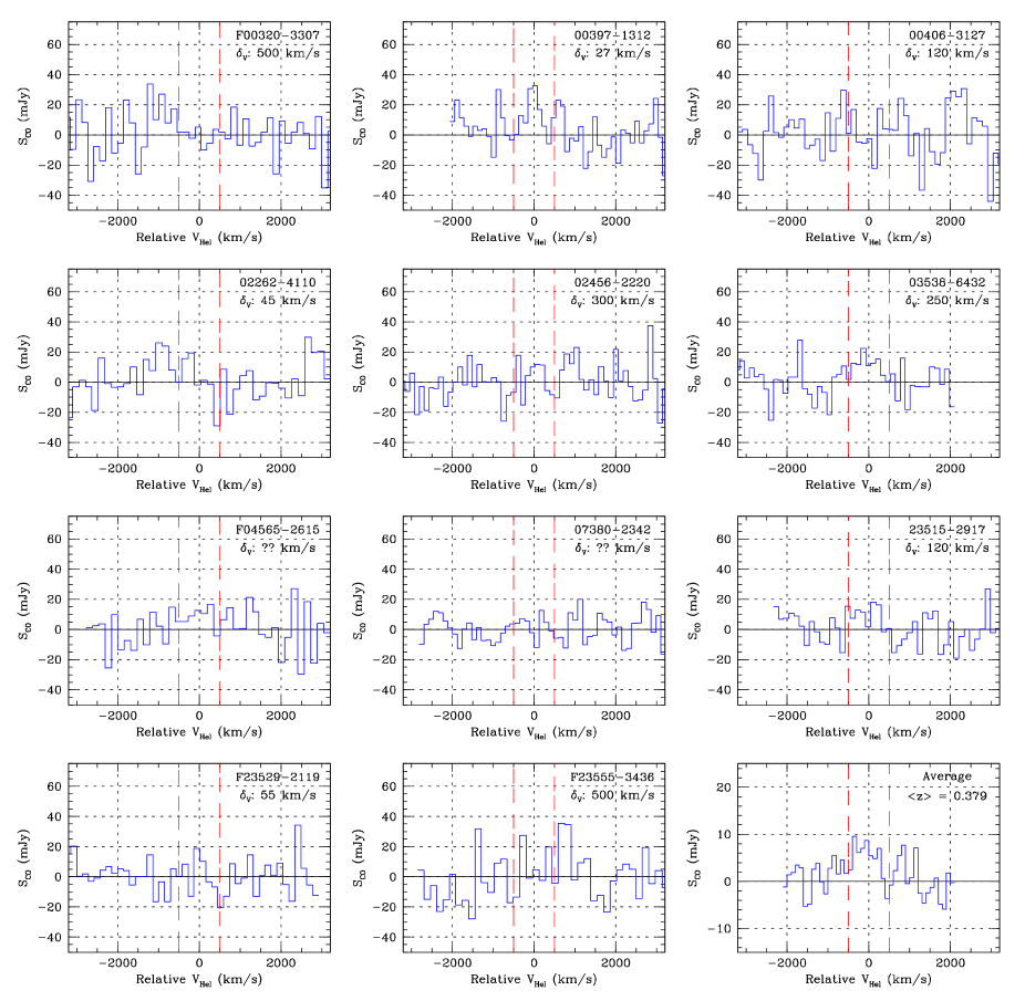
Figure 1: Final spectra of CO(1–0) for the target galaxies in the sample shown at a spectral resolution of about 90 km/s. Vertical lines mark an interval of 1000 km/s centred on the expected systemic velocity. The published uncertainty in the systemic velocity is indicated in each panel. The average stacked spectrum is shown at lower right with the average redshift indicated.

4 Results

Final spectra for each of the observed targets are shown in Fig. 1 at a spectral resolution of about 90 km/s. Vertical lines in this figure mark an interval of 1000 km/s centred on the reference redshift listed in Table 2. The uncertainty in the published redshifts is indicated in each panel. These can be quite substantial. No high significance detections of the redshifted CO(1–0) line were achieved. Upper limits to the integrated line-strength can be calculated by assuming a representative line-width. Detections of CO (1–0) in lower redshift samples of ULIRGs (e.g. Solomon et al. 1997, Chung et al. 2009) suggest that the typical observed linewidth is about 300 km/s. We therefore assumed a more conservative 500 km/s FWHM for the determination of an appropriate noise level. (Flux and mass limits become less restrictive the larger the assumed linewidth.) Since we are searching for the counterpart of a target with known position and velocity, the probability for a false positive detection is given by the tail probability of a standard normal distribution under the assumption of approximately Gaussian noise. A false positive exceeding 2$\sigma$ then has a probability of 0.023. Even for our entire sample size of 11 targets, the false positive rate at this level of significance is only 0.25, which is still significantly less than unity. The 2$\sigma$ upper limits to integrated linestrength were determined from the measured fluctuation level over the entire spectrum (including any possible emission signature) after spectral smoothing to 500 km/s FWHM. The four cases (00397-1312, 03538-6432, F04565-2615 and 23515-2917) where the actual line integral within the central 1000 km/s of the spectrum exceeds this 2$\sigma$ limit are noted as marginal detections in the Table, together with their 1$\sigma$ errors. As noted above, some of the target redshifts have large uncertainties, particularly for F00320-3307 and F23555-3436. In both these cases, there may be evidence for CO emission at an offset velocity that may well be consistent with the current uncertainties in the systemic velocity.

In the lower right panel of Fig. 1 we present the spectrum obtained by aligning all of the measured spectra to relative velocity and forming the simple unweighted average. This yields a high signal-to-noise detection of the mean CO(1–0) line from our sample, as noted in Table 2.

The corresponding line luminosity is given by,

$$L_{CO}=\frac{4\pi D_{L}^{2}\nu_{0}}{c(1+z)}\int S(V)dV$$ (1)

or

$$L_{CO}=1.04\cdot 10^{-3}\frac{D_{L}^{2}\nu_{0}}{(1+z)}S_{V}\ \ \ (L_{\sun})$$ (2)

for the luminosity distance, $D_{L}$, in Mpc, the rest frequency, $\nu_{0}$, in GHz and the integrated linestrength, $S_{V}$, in Jy-km/s. Some authors make use of the quantity,

$$L^{\prime}_{CO}=\frac{c^{2}}{2k_{B}\nu_{0}^{2}}\frac{D_{L}^{2}}{(1+z)}\int S(V)dV$$ (3)

or

$$L^{\prime}_{CO}=3.26\cdot 10^{7}\frac{D_{L}^{2}}{\nu_{0}^{2}(1+z)}S_{V}\ \ \ \mathrm{(K-km/s\ pc^{2})}$$ (4)

with $D_{L},\nu_{0}$ and $S_{V}$ as defined above. For the CO(1–0) transition these measures are related simply by, $L^{\prime}_{CO}/L_{CO}=2.05\cdot 10^{4}$ (K-km/s pc²)/L_☉. The utility of the $L^{\prime}_{CO}$ measure is that it permits more direct comparison of different line transitions since it is formulated as a product of brightness temperature with surface area (Solomon et al., 1997). Line emission of the same brightness temperature originating from the same region will yield the same $L^{\prime}_{CO}$, independent of transition or observing frequency.

Calculation of an associated total hydrogen mass requires an assumed relationship between this quantity and the CO(1–0) line luminosity. A good compilation of such conversion factors is given in Fig. 10 of Tacconi et al. (2008). There is clearly a large scatter in the derived conversion factors and there may well be underlying dependancies on many physical factors, including metallicity, gas surface density and particularly gas excitation temperature. A plausible conversion factor appropriate for ULIRGs is likely to be about 1 M_☉ per (K-km/s pc²) or about $2\cdot 10^{4}$ M_☉ per L_☉.

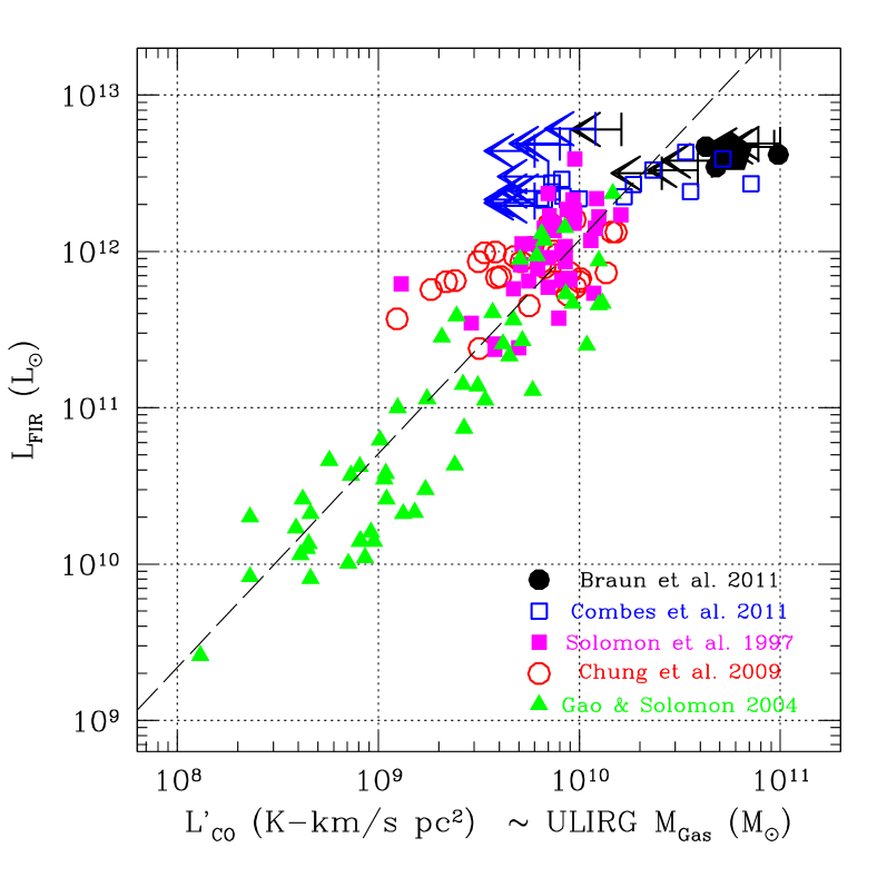
Figure 2: The relationship between CO(1–0) and FIR luminosity. Our results are indicated with the filled circles and 2$\sigma$ upper limit symbols. The large filled pentagon represents our “stacked” result. A power law of slope 1.37$\pm$0.06 represents a least squares fit to the low redshift samples and has a correlation coefficient 0.891.

We plot the distribution of CO(1–0) and FIR luminosity in Fig. 2, including both our own results and those of Combes et al. (2011) as well as previously published studies of less distant and less luminous systems by Solomon et al. (1997), Chung et al. (2009) and Gao & Solomon (2004), all of which have been undertaken in the CO(1–0) transition. Although the low redshift data lie on a well-defined locus in the plot, the intermediate redshift data from both the current study and that of Combes et al. (2011) show divergence from this simple correlation. A subset of the detections has a significant excess CO luminosity, while another subset consisting primarily of upper limits in CO, is significantly underluminous. The difference in CO luminosity between these two populations is about one order of magnitude. A power-law with slope of 1.37$\pm$0.06 has been fit by least squares to the three low redshift samples and is overlaid in the figure. The correlation coefficient of the data points is 0.891. As noted by previous authors (eg. Chung et al., 2009), this relationship is steeper than linear. A single power-law slope provides a reasonable representation of this correlation for FIR luminosities $9.3<\log(L_{FIR})<12.2$. As noted previously, the associated gas mass for a given CO(1–0) line luminosity is likely to vary with the gas kinetic and excitation temperatures, while $L_{FIR}$ is expected to be very sensitive to the dust temperature, $T_{D}$, possibly varying as $T_{D}^{4-6}$ (Soifer et al., 1989).

Gao & Solomon (2004) have demonstrated a higher degree of correlation of $L_{FIR}$ with $L^{\prime}_{CO}$ once a correction of the FIR luminosity for a varying dust temperature has been accounted for. The dust temperature can be estimated from the FIR photometry if an emmissivity law is assumed. This is often taken to be that of a Planck function multiplied by $\nu^{\beta}$, for frequency, $\nu$, and power law exponent, $\beta$. Lisenfeld et al. (2000) have found that the spectral energy distributions (SEDs) in their sample of FIR luminous galaxies could be fit with $0.85~{}<~{}\beta~{}<~{}1.9$. The dust temperature, in the Wien approximation, can be estimated from the ratio, $R_{S}~{}=~{}S_{1}/S_{2}$, of flux densities at two fixed observing frequencies, $\nu_{1}$ and $\nu_{2}$ from,

$$R_{S}=R_{\nu}^{\beta+3}exp\bigg{(}\frac{h(1+z)(\nu_{2}-\nu_{1})}{kT_{D}}\bigg{)}$$ (5)

where $R_{\nu}~{}=~{}\nu_{1}/\nu_{2}$. For the 60 and 100 $\mu$m IRAS bands this yields,

$$T_{D}=\frac{41.7(1+z)}{0.22(\beta+3)-\log(R_{S})}\ \ \ (K)$$ (6)

Since the integrated FIR luminosity is expected to scale as $T_{D}^{\beta+4}$, we have considered normalisations of the FIR luminosity down to a reference temperature of 25 K using the form,

$$L^{\prime}_{FIR}=L_{FIR}\bigg{(}\frac{T_{D}}{25}\bigg{)}^{-(\beta+4)}$$ (7)

The case has also been made that the CO(1–0) line luminosity would vary approximately linearly with $T_{D}$ (Solomon et al., 1997) if the dust and gas temperatures are reasonably coupled, suggesting a similar normalisation of the form,

$$L^{\prime\prime}_{CO}=L^{\prime}_{CO}\bigg{(}\frac{T_{D}}{25}\bigg{)}^{-\alpha}$$ (8)

We find empirically,that the values $(\alpha,\beta)$ = (1,1) minimise the dispersion in the temperature-normalised CO(1–0) versus FIR luminosity relationship. The resulting relation is illustrated in Fig. 3, where a power-law of slope 0.99$\pm 0.04$ has been fit by least squares to the three low redshift samples. The correlation coefficient with this choice of $(\alpha,\beta)$ is 0.902. A very similar relation, with a slope 1.03$\pm 0.05$, is obtained for $(\alpha,\beta)$ = (1,1.5), which may be more representative of the FIR SEDs (Lisenfeld et al., 2000). The distinction between the CO-luminous and CO-poor populations is undiminished in the temperature corrected relationship.

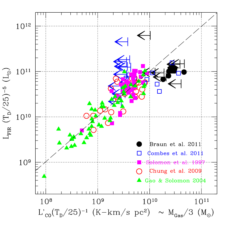
Figure 3: The relationship between temperature normalised CO(1–0) and FIR luminosity. $L_{CO}$ is normalised by $(T_{D}/25)^{1}$ and $L_{FIR}$ by $(T_{D}/25)^{5}$, for a reference dust temperature, $T_{D}$ = 25 K. A power law of slope 0.99$\pm 0.04$ represents a least squares fit to the low redshift samples and has a correlation coefficient 0.902. A similar fit is achieved for $L_{CO}$ normalised by $(T_{D}/25)^{1}$ and $L_{FIR}$ by $(T_{D}/25)^{5.5}$.

We can estimate the dust mass associated with our targets from,

$$M_{D}=\frac{S_{\nu 0}D_{L}^{2}}{(1+z)\kappa_{\nu z}B_{\nu z}(T_{D})}$$ (9)

where $S_{\nu 0}$ is the observed flux density in an FIR band, $D_{L}$ is the luminosity distance, $\kappa_{\nu z}$ is the absorption cross section per unit dust mass at the target rest-frame frequency $\nu_{z}=\nu_{0}(1+z)$ and $B_{\nu z}(T_{D})$ is the Planck function at this frequency for a dust temperature, $T_{D}$ (Hildebrand, 1983). The dust absorption cross section can be approximated by,

$$\kappa_{\lambda}=27.2\bigg{(}\frac{\lambda_{\mu m}}{100}\bigg{)}^{-2.15}\big{(}1+0.625[\log(\lambda_{\mu m})-2.15]^{2}\big{)}$$ (10)

in units of cm²/g for wavelengths expressed in $\mu$m between 40–1000 $\mu$m. This analytic form fits the tabulated data of Draine (2003) to better than 5% over the indicated wavelength range. We calculate the dust masses for our sample and the comparison samples noted previously using the observed IRAS 100 $\mu$m fluxes and the dust temperatures calculated with eqn. 6 and $\beta~{}=~{}1.5$, listing these in Table 2.

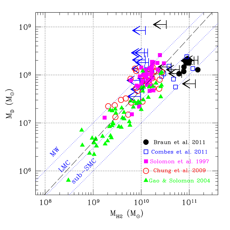
Figure 4: The relationship between molecular hydrogen mass and dust mass. A power law of slope 1.09$\pm 0.05$ is shown as a dashed line and represents a least squares fit to the low redshift samples and has a correlation coefficient 0.893. Dotted lines labelled with sub-SMC, LMC and MW represent increasing dust-to-molecular hydrogren mass ratios of 0.001, 0.003 and 0.01 respectively.

Once the CO luminosity has been temperature-corrected, it seems more likely that a single conversion factor to total molecular hydrogen mass, appropriate to the 25 K reference temperature, might apply. From Tacconi et al. (2008) this might correspond to about 3 M_☉ per (K-km/s pc²) or about $6\cdot 10^{4}$ M_☉ per L_☉. Even so, there may well be other systematic dependancies and a large intrinsic scatter, that add significant uncertainty to this conversion factor. The relationship between molecular hydrogen mass and dust mass is shown in Fig. 4. A power-law fit to the low redshift samples has slope 1.09$\pm 0.05$ and a correlation coefficient of 0.893 and is plotted in the Figure. Also shown are diagonal lines corresponding to fixed dust to hydrogen mass ratios of 0.001, 0.003 and 0.01, which are labelled sub-SMC, LMC and MW respectively (cf. Draine et al., 2007). The sub-SMC designation is used for the lowest curve since the Small Magellanic Cloud is estimated to have a mass ratio of 0.002 (eg. Weingartner & Draine, 2001). The correlated locus in Fig. 4 defined by the low redshift samples systematically increases in dust-to-gas mass ratio with increasing gas mass, from SMC-like values at the low end, through Large Magellanic Cloud and up to Milky Way values for $M_{H_{2}}>10^{10}$ M_⊙.

What is striking in Fig. 4 is that all of the intermediate redshift detections in both the current and Combes et al. (2011) studies depart from the low redshift trend in the direction of extremely low dust-to-molecular gas mass ratio. Our well-defined sample average point of 0.0021$\pm$0.0002 is comparable to the dust-to-hydrogen mass ratio of the SMC. In contrast, there are several upper limits in the figure which appear to be dust-rich (or gas-poor) by about an order of magnitude. The most extreme point from the current sample is the source IRAS 0738-2342, while in the Combes et al. (2011) sample it is IRAS 19104+8436. Two addtional sources in the Northern sample, [HB89] 1821+643 and F 00415-0737, are also discrepant but less extreme. While very little is currently known about F 00415-0737, Ruiz et al. (2010) have recently presented SED fits for IRAS 0738-2342 and [HB89] 1821+643. They estimate relative AGN:Starburst contributions to the bolometric luminosity of about 50:50 and 80:20 for these two sources. Both IRAS 19104+8436 and [HB89] 1821+643 are classified as Seyfert 1/QSOs, suggesting that $L_{FIR}$ for IRAS 19104+8436 may also be dominated by non-thermal rather than dust emission.

It seems plausible that the apparent “gas poor” sub-population seen at intermediate redshift in Figs. 2,  3 and  4 may simply be a manifestation of AGN contamination, with the star formation dominated population demonstrating a well-defined trend relative to the low redshift samples, consistent with a dramatic decline in the dust-to-molecular gass mass ratio.

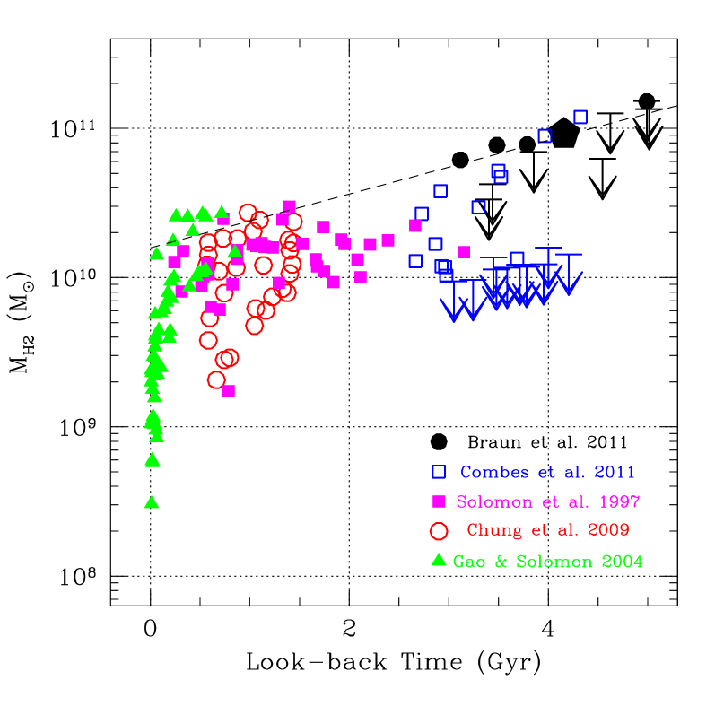
Figure 5: The relationship between look-back time and ULIRG molecular hydrogen mass. An indicative upper envelope to molecular gas mass, $\log(M_{H_{2}})=10.2+0.18\tau$, is plotted demonstrating the order of magnitude decline in maximum ULIRG gas mass over the past 5 Gyr.

We consider the distribution of ULIRG molecular hydrogen mass with look-back time, $\tau$, in Fig. 5. Since ULIRGs are identified by their extreme luminosity in the FIR band, where self-opacity and foreground extinction effects are minimal, they represent a population that is easily recognised in unbiased surveys of the sky. Both our own study, as well as the others shown in the Figure, were drawn from the most luminous soures in the IRAS all-sky survey. As such they are not expected to suffer from incompleteness at high luminosity and despite the fact that they are a rare population, they permit a useful assessment of the associated molecular gas mass that is required to feed the ULIRG phenomenon. Although the lowest detected gas masses at each look-back time simply reflect the sensitivity of the observation and the cutoff $L_{FIR}$ of the sample, the upper envelope to mass in Fig. 5 is a significant attribute of the population, at least once the sample extends over a representative volume of about 10⁷ Mpc³; since the most luminous sources are clearly the easiest to detect at any redshift. This condition should be met for redshifts greater than about 0.03, or look-back times exceeding 0.4 Gyr. This local volume saturation effect is apparent in the Figure for $\tau<0.5$ Gyr. The indicative curve drawn in the Figure,

$$\log(M_{H_{2}})=10.2+0.18\tau$$ (11)

demonstrates the order of magnitude decline in maximum molecular gas mass of the ULIRG population during the past 5 Gyr. Such a decline is comparable to, but even more dramatic, than that seen in the star formation rate density (Hopkins & Beacom, 2006) which can be well described by,

$$\log(\dot{\rho}_{*})=-1.76\pm 0.02+0.131\pm 0.004\tau$$ (12)

for a star formation rate density $\dot{\rho}_{*}$ in M_⊙yr^-1Mpc^-3 for $\tau<$ 8 Gyr. This contrast suggests significant changes in the molecular gas mass function at even these modest look-back times.

We will present further analysis of the time evolution of molecular gas and other baryonic constituents of galaxies in a subsequent publication.

References

- Chung et al. (2009) Chung, A., Narayanan, G., Yun, M.S., Heyer, M., Erickson, N.R., 2009, AJ, 138, 858
- Combes et al. (2011) Combes, F., Garcia-Burillo, S., Braine, J., Schinnerer, E., Walter, F., Colina, L., 2011, A&A, 528, 124
- Dickman et al. (1986) Dickman, R.L., Snell, R.L., Schloerb, F.P. Solomon, 1986, ApJ, 309, 326
- Draine (2003) Draine, B.T., 2003, ARAA, 41, 241
- Draine et al. (2007) Draine, B.T., Dale, D.A., Bendo, G., et al., 2007, ApJ, 663, 866
- Gao & Solomon (2004) Gao, Y., Solomon, P.M., 2004, ApJ, 606, 271
- Geach et al. (2009) Geach, J.E., Smail, I., Coppin, K., et al., 2009, MNRAS, 395, L62
- Geach et al. (2011) Geach, J.E., Smail, I., Moran, S.M., et al., 2011, ApJ, 730, L19
- Genzel et al. (2010) Genzel, R., Tacconi, L.J., Gracia-Carpio, J., et al. 2010, MNRAS, 407, 2091
- Heavens et al. (2004) Heavens, A., Panter, B., Jimenez, R., Dunlop, J., 2004, Nature, 428, 625
- Hildebrand (1983) Hildebrand, R.H., 1983, QJRAS, 24, 267
- Hinshaw et al. (2009) Hinshaw, G., Weiland, J.L., Hill, R.S., et al., 2009, ApJS, 180, 225
- Hopkins & Beacom (2006) Hopkins, A.M., Beacom, J.F., 2006, ApJ, 651, 142
- Ivison et al. (2011) Ivison, R.J., Papadopoulos, P.P., Smail, I., etal., 2010, MNRAS, 412, 1913
- Keres et al. (2003) Keres, D., Yun, M.S., Young, J.S., 2003, ApJ, 582, 659
- Ladd et al. (2005) Ladd, N., Purcell, C., Wong, T., Robertson, S., 2005, PASP, 22, 62
- Lisenfeld et al. (2000) Lisenfeld, U., Isaak, K.G., Hills, R., 2000, MNRAS, 312, 433
- Riechers et al. (2010) Riechers, D.A., Carilli, C.L., Walter, F., Momjian, E., ApJ, 714, L153 Soifer, B.T., Boehmer, L., Neugebauer, G., Sanders, D.B., 1989, AJ 98, 766
- Ruiz et al. (2010) Ruiz, A., Miniutti, G., Panessa, F., Carrera, F.J., 2010, A&A, 515, A99
- Sanders & Mirabel (1996) Sanders, D.B., Mirabel, F., 1996, ARAA, 34, 749
- Soifer et al. (1989) Soifer, B.T., Boehmer, L., Neugebauer, G., Sanders, D.B., 1989, AJ, 98, 766
- Solomon et al. (1997) Solomon, P.M., Downes, D., Radford, S.J.E., Barrett, J.W., 1997, ApJ, 478, 144
- Tacconi et al. (2008) Tacconi, L.J., Genzel, R., Smail, I. et al., 2008, ApJ, 680, 246
- Ulich & Haas (1976) Ulich, B.L., Haas, R.W., 1976, ApJSS, 30, 247
- Weingartner & Draine (2001) Weingartner, J.C., Draine, B.T., 2001, ApJ, 548, 296