What do cluster counts really tell us about the Universe?
Abstract
We study the covariance matrix of the cluster mass function in cosmology. We adopt a two-line attack: firstly, we employ the counts-in-cells framework to derive an analytic expression for the covariance of the mass function. Secondly, we use a large ensemble of -body simulations in the CDM framework to test this. Our theoretical results show that the covariance can be written as the sum of two terms: a Poisson term, which dominates in the limit of rare clusters; and a sample variance term, which dominates for more abundant clusters. Our expressions are analogous to those of Hu & Kravtsov (2003) for multiple cells and a single mass tracer. Calculating the covariance depends on: the mass function and bias of clusters, and the variance of mass fluctuations within the survey volume. The predictions show that there is a strong bin-to-bin covariance between measurements. In terms of the cross-correlation coefficient, we find for haloes with at . Comparison of these predictions with estimates from simulations shows excellent agreement. We use the Fisher matrix formalism to explore the cosmological information content of the counts. We compare the Poisson likelihood model, with the more realistic likelihood model of Lima & Hu (2004), and all terms entering the Fisher matrices are evaluated using the simulations. We find that the Poisson approximation should only be used for the rarest objects, , otherwise the information content of a survey of size would be overestimated, resulting in errors that are 2 times smaller. As an auxiliary result, we show that the bias of clusters, obtained from the cluster-mass cross-variance, is linear on scales , whereas that obtained from the auto-variance is nonlinear.
1. Introduction
The last decade of research in cosmology has largely been focused on devising probes to reveal the physical nature of dark energy and the origin of the accelerated expansion of the Universe. Among the most promising probes, as identified for example in Albrecht et al. (2006), are cluster counts.
From a theoretical perspective, the abundance of clusters per unit solid angle , is an integral of the mass function over mass and volume element :
| (1) |
where is a redshift-dependent mass detection threshold for the clusters and where the mass function is defined as the number of halos per unit volume and unit mass, i.e. , with the virial mass. For a wide range of cosmological models, can be accurately predicted from the semi-analytical prescriptions based on the spherical or ellipsoidal collapse model (e.g. Press & Schechter, 1974; Sheth & Tormen, 1999, and see §3.4 for more details.).
The mass function is primarily sensitive to the statistics of the initial conditions and to the amplitude and shape of the matter power spectrum; which in turn depends on the matter density of the Universe , the Hubble parameter , the spectral index of the primordial power spectrum ; and the dark energy equation of state , where and are the pressure and energy density of the dark energy. The volume element integral in the above equation renders the cluster counts even more sensitive to and . Measuring the cluster abundance at different redshifts can constrain a dynamical and thus enable one to differentiate between a cosmological constant and alternative dark energy scenarios such as quintessence (Wang & Steinhardt, 1998), or dark energy inhomogeneities coupling to dark matter (Manera & Mota, 2006).
For many decades the study of clusters of galaxies has been a centerpiece for observational cosmology, which has produced many important results and cosmological inferences. Currently there are four observational strategies for detecting clusters: -ray emission (see Borgani et al., 2001; Reiprich & Böhringer, 2002; Schuecker et al., 2003; Allen et al., 2003; Henry, 2004; Mantz et al., 2008; Vikhlinin et al., 2009; Mantz et al., 2010, and references therein); optical emission (see Gladders et al., 2007; Rozo et al., 2010, and references therein); the Sunyaev–Zel’Dovich effect (Sunyaev & Zeldovich, 1972, hereafter SZ effect), i.e. the up-scattering of CMB photons off hot electrons in the intracluster medium (see Vanderlinde & The SPT Collaboration, 2010; Planck Collaboration et al., 2011; Muchovej et al., 2011; Sehgal & The ACT Collaboration, 2011, and references therein); weak gravitational lensing (see Schirmer et al., 2007; Abate et al., 2009; Israel et al., 2010, and references therein).
One of the most challenging aspects of deriving cosmological constraints from cluster counts is the fact that virial masses are not directly observable: a conversion is needed to translate observables such as flux, luminosity, temperature and SZ decrement into mass. The mass-observable relation is degenerate with cosmological parameters, as shown in Lima & Hu (2005), and can severely degrade the inferred constraints. Substantial progress has been made in calibrating the mass-observable relation in the recent years, through numerical simulations, or by comparing different methods against each other (Zhang et al., 2007, 2008; Okabe et al., 2010). Lima & Hu (2005) also proposed a self-calibration technique that uses the clustering of clusters to break the degeneracy between the uncertainties in the mass-observable relation and cosmological parameters.
Owing to observational challenges, the cluster studies mentioned earlier employ small numbers of massive clusters (at most a few hundreds, but in general a few tens) to constrain cosmology. In obtaining these constraints it is widely assumed that the likelihood function for the selected clusters follows the Poisson distribution. Whilst this assumption may be reasonable for the most massive clusters, , it will certainly fail at lower masses. Future surveys, such as eROSITA (Predehl et al, 2010), LSST (2009), Euclid (Refregier et al., 2010), Pan-STARRS111http://pan-starrs.ifa.hawaii.edu, DES (2005), will be able to detect large samples of intermediate-mass clusters, . In order to make accurate inferences from this data, the cluster likelihood function will require a more complex statistical treatment, and in particular knowledge about the covariance matrix of the mass function.
This paper is driven by the following two questions: What is the covariance matrix for measurements of the mass function? How much are forecasted errors, which rely on the Poisson approximation, affected by more realistic modelling of the cluster likelihood function? The main theoretical tools that we shall employ to answer these questions will be the counts-in-cell formalism introduced by Peebles (1980) and further developed by Hu & Kravtsov (2003, hereafter HK03) and Lima & Hu (2004, hereafter LH04). We shall also compare the theoretical results obtained via this formalism to measurements obtained from a large ensemble of -body simulations.
As this paper was nearing submission, a study by Valageas et al. (2011) was reported. This work explores related, but complimentary, questions to those presented here.
The paper is structured in the following way: in §2 we review the counts-in-cells formalism and also the extension to the cluster likelihood developed by LH04; in §3 we derive the mass function covariance in a formal way; in §4 we describe the numerical simulations from which we measure the mass function covariance; in §5 we present a comparison between the measured and the predicted covariance, and in §6 we use the Fisher-matrix formalism to estimate the impact that the full covariance matrix of the mass function has on cosmological constraints. Finally, in §7 we discuss and summarize our findings.
2. Theoretical background
2.1. The cellular model
In this section, we give a short description of the counts-in-cell formalism, used by HK03 to compute the linear-theory sample variance of cluster counts, and by LH04 to estimate the impact of the latter on Fisher matrix predictions.
Consider some large cubical patch of the Universe, of volume , and containing clusters that possess some distribution of masses. Let us subdivide this volume into a set of equal cubical cells and the mass distribution into a set of mass bins. Let the number of clusters in the cell and in the mass bin be denoted . We shall assume that the probability that the cell contains clusters in the mass bin , is a Poisson process:
| (2) |
For any quantity , we denote the average over the sampling distribution–the Poisson process in this case–as , and the ensemble average over many realizations of the density field as , termed sample variance in HK03. The average of over the sampling distribution can be written as (see also Cole & Kaiser, 1989; Mo & White, 1996):
| (3) |
where is the ensemble- and Poisson-averaged number of counts in cell and mass bin . The volume of the cell and the cell-averaged overdensity are given by,
| (4) | |||||
| (5) |
where is the window function for the th cell (see §3.2 for more details). The number density and linear bias of the clusters averaged over the mass bin are given by:
| (6) | |||||
| (7) |
where is the linear bias of haloes of mass .
As was shown in HK03, the correlations in the underlying density field induce a correlation in the number counts of the cells, defined as:
| (8) | |||||
where for independent Poisson processes the probability . In the last line we introduced the power spectrum as the Fourier transform of the correlation function ,
| (9) |
is the Fourier transform of the cell window function and (see §3.2).
2.2. The Gauss-Poisson likelihood function for counts in cells
The likelihood of drawing a particular set of cluster counts in the cells, given a model for the counts in the cells was written by LH04:
| (10) |
with , and where it was assumed that the statistics of the cell-averaged density field are described by a multivariate Gaussian:
| (11) |
with defined in Eq. (8). Measurements of the bispectrum of the CMB have shown that the statistics of the initial fluctuations are very nearly Gaussian (Komatsu et al., 2010). Whilst we know that nonlinear growth of structure in the present epoch drives the statistics of the density field to become non-Gaussian, in the limit that the cells are large compared to the coherence length of the field, we expect that the Gaussian approximation will be very good.
At this point we may also be more precise about what we mean by ensemble and Poisson averages:
| (12) |
Equation (10) can be simplified in two limits:
-
•
Case I: In the limit that the ensemble average variance is much smaller than the Poisson variance: i.e. . In this case, the Gaussian effectively becomes a delta function centred on and the likelihood simply becomes a product of Poisson probabilities:
(13) -
•
Case II: In the limit that the number of counts in each cell and mass bin is large, then the Poisson process becomes a Gaussian:
(14) where . Hence, as shown in LH04, the likelihood function becomes,
(15) and via the convolution theorem this can be approximated as a Gaussian with shifted mean and augmented covariance matrix:
(16) where . Note that in the above equation, the approximate sign is used since negative number counts are formally forbidden (for a more detailed discussion of this see Hu & Cohn, 2006).
3. Covariance of the mass function
The final result of §2 is that in the limit of a large number of counts per cell, the joint likelihood for all the cells is a Gaussian with model mean and with a covariance matrix, . In the following section, we shall use these results to answer the question: What is the covariance matrix for measurements of the mass function?
3.1. A formal approach
The mass function is the number density of clusters in a volume , per unit mass. Using our counts in cells distribution, an estimator for the mass function in the cell is,
| (17) |
which, if we average over all cells and all cells have equal volume, becomes
| (18) |
The above estimate is unbiased, and its expectation value can be formally calculated using Eq.(12):
| (19) | |||||
In a similar fashion, the covariance matrix of the cluster mass function can also be calculated:
| (20) | |||||
where the expectation of the product of the counts can be written
Recall that and that for the Poisson distribution we have: . On inserting these relations into the above equation, and on completing the sums, we find:
| (22) | |||||
where in the last line we used Eq. (8). On inserting this result back into Eq. (20), we obtain
| (23) | |||||
Considering the first term in the above, we may simplify this expression by performing the sums over and , and the window functions i.e.
Hence, we have that the covariance matrix can be written:
| (25) |
where is the mass density variance in the entire volume
| (26) |
From Eq. (25) it can be seen that the crucial quantity which controls the covariance between estimates of the mass function in different mass bins is . The strength of the covariance is also modulated by the linear bias and the mass function in each of the bins considered.
3.2. A short-cut to the covariance
Whilst in the above we have presented a formal derivation of the mass function covariance from the HK03 and LH04 formalism, there is a more intuitive approach to arriving at the same result as given by Eq. (25), which we now mention.
Let us consider the limiting case where we have a single cell that fills the whole of our sample space ; also and similar for all the other quantities defined in the cells. The above formalism still applies, and we have that the covariance matrix of mass function can be written:
| (27) | |||||
where is the variance in the total volume.
3.3. The cross-correlation coefficient
As a direct corollary to the previous results, we may write an expression for the correlation matrix, which is defined
| (28) |
On factoring out from in the denominator, and a similar term from , and on using the fact that , we find
| (29) |
Two limits are apparent: when , then and the mass function covariance matrix is decorrelated; this would happen for the case of rare halos, for which the mass function is very small. On the other hand, when , then and the covariance matrix is fully correlated. This would be the case for smaller halos, for which the mass function is quite large.
Finally, we note that taking and hence , does not guarantee that the correlation between different mass bins is negligible. As the above clearly shows, it is the quantity that is required to vanish for negligible correlation to occur. For a power-law power spectrum, we would have that , which only vanishes for . For CDM we have a rolling spectral index, and for , which implies that for the covariance to diminish.
At this juncture, we point out that Eqs (25) and (29) constitute the main analytic results of this work, and all which follows will be concerned with their validation and implications.
| Cosmological parameters | |||||||
|---|---|---|---|---|---|---|---|
| zHORIZON-I | 0.25 | 0.75 | 0.04 | -1 | 0.8 | 1.0 | 70.0 |
| zHORIZON-V1a/V1b | 0.25 | 0.75 | 0.04 | -1 | 0.8 | 0.95/1.05 | 70.0 |
| zHORIZON-V2a/V2b | 0.25 | 0.75 | 0.04 | -1 | 0.7/0.9 | 1.0 | 70.0 |
| zHORIZON-V3a/V3b | 0.2/0.3 | 0.7 | 0.04 | -1 | 0.8 | 1.0 | 70.0 |
| zHORIZON-V4a/V4b | 0.25 | 0.8 | 0.04 | -1.2/-0.8 | 0.8 | 1.0 | 70.0 |
| Simulation Parameters | ||||||
|---|---|---|---|---|---|---|
| zHORIZON-I | 1500 | 60 | 40 | 135 | ||
| zHORIZON-V1, -V2, -V4 | 1500 | 60 | 4 | 13.5 | ||
| zHORIZON-V3a | 1500 | 60 | 4 | 13.5 | ||
| zHORIZON-V3b | 1500 | 60 | 4 | 13.5 |
3.4. Ingredients for evaluating the covariance
To evaluate the covariance matrix we need to provide models for , and the Fourier transform of the survey window function.
To compute and we employ the mass function and bias models presented in Sheth & Tormen (1999):
| (30) |
| (31) |
| (32) |
where . In the above we have introduced the peak-height , where is the spherical overdensity for collapse, and where is the variance of the linear density field extrapolated to , smoothed with a spherical top-hat filter of radius (see below for more details). This radius is defined so as to enclose a mass , with the mean matter density of the Universe at the present epoch.
For the survey window function we shall consider two simple examples. The first is a cubical top-hat, defined by:
where denotes the Cartesian components of the vectors, is the cell index, and is the size of the cell of volume . The Fourier transform of this top-hat window function is:
| (33) |
where is the zeroth order spherical Bessel function. The volume variance for this window function is:
| (34) | |||||
where in the second equality we have used the isotropy of the power spectrum, e.g. . In Eq. (34) we use the following relation:
| (35) |
The second window function is a spherical top-hat:
| (37) |
where is the radius of the spherical top-hat. The variance of the density field in this case has the familiar form:
| (38) |
for which the Fourier transform is given by:
| (39) |
On a technical note, we point out that for the -space integrals given by Eqs (34) and (38), we have introduced lower and upper limits and , respectively. For a real survey, the upper limit is decided by the resolution of the instrument used. If the measurements are made from numerical simulations, which is the case with this work, the softening length of the simulations will dictate the largest frequency Fourier mode available: and for our simulations . However, in practice the largest useful Fourier mode is much smaller, and occurs where the shot-noise correction to the power spectrum becomes comparable with the signal (Smith et al., 2003).
The lower limit is a more complex issue. In the case of simulations, no modes with wavelength larger than the simulation box can contribute to the variance, which suggests the straightforward solution of adopting . Since we are attempting to confront the theory with the reality defined by simulations, we shall always assume this cut-off scale. However, for real surveys, the variance on a given scale will be affected by the existence of modes on scales larger than the size of the survey. We therefore recommend in this case , or at least the inverse horizon size at the redshift of the survey. For more discussion of the importance of for the predictions of the variance, see discussion in Appendix A.
Note that in the above we shall relate the radius of the spherical top-hat to that of the cubical top-hat function, through the relation . In other words the volumes of the spherical and cubical sample volumes are taken to be identical.
4. -body simulations
We study the covariance matrix with a suite of 40 large numerical simulations, executed on the zBOX-2 and zBOX-3 supercomputers at the Institute for Theoretical Physics, University of Zürich. For all realizations snapshots were output at: . We shall refer to these simulations as the zHORIZON Simulations.
Each of the zHORIZON simulations was performed using the publicly available Gadget-2 code (Springel, 2005), and followed the nonlinear evolution under gravity of equal-mass particles in a comoving cube of length . The cosmological model is similar to that determined by the WMAP experiment (Komatsu et al., 2009). We refer to this cosmology as the fiducial model. The transfer function for the simulations was generated using the publicly available cmbfast code (Seljak & Zaldarriaga, 1996; Seljak et al., 2003), with high sampling of the spatial frequencies on large scales. Initial conditions were set at redshift using the serial version of the publicly available 2LPT code (Scoccimarro, 1998; Crocce et al., 2006). Table 1 summarizes the cosmological parameters that we simulate and Table 2 summarizes the numerical parameters used.
In this paper we also study the Fisher matrix of cluster counts for which we use another series of simulations. Each of the new set is identical in every way to the fiducial model, except that we have varied one of the cosmological parameters by a small amount. For each new set we have generated 4 simulations, matching the random realization of the initial Gaussian field with the corresponding one from the fiducial model. The four parameter variations that we consider are , and we refer to each of the sets as zHORIZON-V1a,b,…,zHORIZON-V4a,b, respectively. Again, the full details are summarized in Tables 1 & 2.
Lastly, dark matter halo catalogues were generated for all snapshots of each simulation using the Friends-of-Friends (FoF) algorithm (Davis et al., 1985), with the standard linking-length parameter , where is the fraction of the inter-particle spacing. For this we employed the fast parallel B-FoF code, kindly provided to us by V. Springel. The minimum number of particles for which an object is considered to be a bound halo was set at 20 particles. This gave a minimum host halo mass of .

5. Results
In this section we confront the counts-in-cells theory with the results from -body simulations.
5.1. Cell variance in simulations and theory
Since plays a vital role in determining the strength of any covariance in the mass function measurements, we shall make a detailed study of it, for both window functions discussed in §3 and considering volumes of varying size. We evaluate in two different ways, analytically and from -body simulations. Furthermore, owing to concerns regarding the impact of nonlinear bias and mass evolution, we also compute the matter-matter, halo-matter, and halo-halo variance, which we denote as , and , respectively. Comparing these quantities will then make clear any departures from linearity.
Our analytical approach to determining the variances is based on standard quadrature routines to evaluate the theoretical expressions: for Eq. (34), we use the multi-dimensional Monte-Carlo integration routine VEGAS; and for Eq. (38), we use the QROMB routine (for more details see Press et al., 1992). In evaluating these integrals we take the linear theory power spectrum matching our simulations, fully described in §4. Also, we take the largest mode in the simulation box to determine the lower limit of the -integrals .
The second method is one of brute force: we measure , and directly from the ensemble of simulations. Our estimator for the variances can be expressed as:
| (40) | |||||
where the indices label the Fourier mesh cell and the magnitude of the wavenumber corresponding to that cell. The total number of grid cells considered is ; also, and are , and are estimates of the various auto- and cross-power spectra. The window functions are as given in §3. The estimates of the variance also require a correction for shot-noise, which for the halo-halo variance we implement in the following way:
| (41) |
where is the number of halos in the considered mass bin, and and are the variance of the continuous and discrete halo density fields, respectively. There is a similar shot-noise correction for the matter-matter variance; we assume that the halo-mass cross-variance requires no such correction. Note that the above method for estimating is not the conventional one, where one partitions the real space counts into cells and then computes the variance of that distribution. However, it should be entirely equivalent, but with the added advantages of being fast, since we are using an FFT, and allowing for the computation of the variance in arbitrary cell structures.
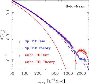
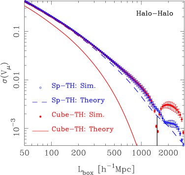
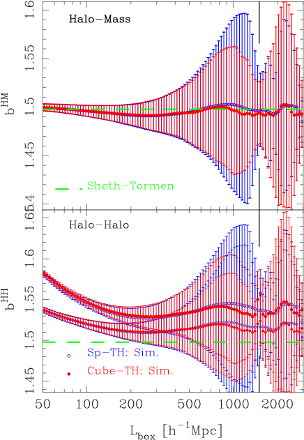
Rather than testing all of the halo mass bins that we will employ later for the mass function covariance, we have chosen to show results for all the haloes in the simulation with . Figure 1 presents our results for , and as a function of the cubical window function size, ; recall that for the spherical window we take the radius to be . In all three panels, the points represent results from the -body simulations, whereas the lines denote the analytical integrals. The red full circles and solid lines are obtained by smoothing the density field with the cubical top-hat, while the blue empty circles and dashed lines denote smoothing with the spherical top-hat function. The simulation results represent the mean of the 40 realizations, with errors appropriate for a single run. The size of the simulation box () is marked through a vertical black line on the horizontal axis. The effects of the shot-noise corrections on the estimates of and are too small to be noticed on this log–log plot.
As expected for a hierarchical mass distribution, in all cases the variance decreases steeply with the increasing box size. On comparing the results obtained from the simulations for the two window functions, we find very good agreement up until the size of the cubical region becomes similar to the size of the simulation cube. At this scale, the variance from the cubical window function displays a significant loss in signal. For scales larger than the simulation box, the smoothing result become somewhat meaningless and unstable due to the oscillatory nature of both window functions, which can be seen from the measurements.
Turning to the evaluation of the theoretical expressions for the variance, we see that, in the case of the spherical top-hat there is excellent agreement between the simulations and the theory on small scales, . For , the linear expressions underestimate the measurements by or even more. However, on comparing the theoretical predictions for the cubical filter function with the measurements, we find a large discrepancy. We tested whether this was due to an error in the VEGAS evaluation of the integrals. An independent check with mathematica produced the same results.
After some investigations, we found that the discrepancy between the simulation and theory results was solely attributable to the difference between the discrete lattice structure of the Fourier space used in the simulations, and the continuum of Fourier modes used in the numerical integrals. A detailed discussion of this is presented in Appendix A.1. In that section we also show that as the simulation box size is increased, the theory and simulation results converge. Further, as is shown in Appendix A.2 the theory predictions are sensitive to the lower limit . In applying this to the real Universe, we suggest letting .
5.2. Linearity of the bias
In linear theory, the relation between the variances plotted in Figure 1 is given by:
| (42) |
is the average linear bias from Eq. (7), estimated for a single mass bin containing all halos larger than . For the theoretical bias, we use the Sheth-Tormen model Sheth & Tormen (1999, 2002), averaged over the same mass bin. All quantities are at redshift 0. Since the bias is , is slightly larger than , which in turn is also slightly larger than . At this level of detail the differences between the curves appear to be well related to each other as in Eq. (42).
To check this more accurately we next estimate the halo bias in the simulations and compare it directly with the theoretical predictions. In direct analogy with the Fourier-space bias estimates in Smith et al. (2007), we construct the following real-space bias estimates:
| (43) |
where all quantities in the above depend on . Figure 2 presents the comparison between the estimates of the linear bias from the simulations and the values obtained from the Sheth-Tormen formula. The top and bottom panels show the results for and , respectively. Again the solid red and empty blue circles denote the results from the cubical and spherical window functions, respectively. The Sheth-Tormen theory is represented by the thick green dashed line.
Considering (top panel), the first thing to remark is that the bias appears extremely flat over all of the scales probed – for the mean of the realizations the bias relation is linear to better than 1% precision. Secondly, the peak-background split model of Sheth & Tormen predicts this value astonishingly well: .
Turning our attention to (lower panel), the raw simulation measurements (upper set of points) indicate that on scales , the bias displays a weak scale-dependence and is roughly higher than the Sheth-Tormen prediction. However, on smaller scales nonlinear effects are apparent and the overall amplitude is steadily increasing with decreasing scale, being higher than the Sheth-Tormen prediction for . The figure also shows the importance of correcting for shot-noise when making estimates of the bias. The upper and lower set of points in this panel denote the uncorrected and corrected estimates, respectively. The shot-noise correction reduces the discrepancy between the simulations and linear theory to within for , however the nonlinearity on smaller scales remains.
Both cubical and spherical window functions yield very similar results. In the rest of this work we shall employ the Sheth-Tormen bias, since on the scales of interest we have shown that it is at worst compared to the average bias of the haloes in our simulations.
Finally, we mention that for the analytical results in the next sections, we shall use: (i) the volume variance measured from the matter-matter power spectrum with a cubical window function, and not the analytical variance, given the discrepancy seen in Figure 1. The cubical window function is a natural choice, since our simulations also have this geometry; (ii) the Sheth-Tormen bias; (iii) the Sheth-Tormen mass function.

5.3. An estimator for the mass function covariance
We estimate the mass function covariance matrix from the ensemble of 40 simulations of the fiducial cosmological model, described in §4. As we will show shortly, this number of realizations is insufficient for a reliable estimate of the covariance matrix. In order to overcome this problem, we have adopted the simple strategy of subdividing the volume associated with each realization into a set of smaller cubes. In particular, we divide each dimension of the original cube by 2, 3, and 4. Hence, each cube of is partitioned into 8, 27, and 64 subcubes with corresponding volumes of , , and , respectively. The ‘subcubing’ procedure thus provides us with 40, 320, 1080, and 2560 quasi-independent realizations. We note that this strategy was also adopted by Crocce et al. (2010), who used it to compute sample-variance error bars on the mass function in the MICE simulations. However, it has never been employed to compute the covariance matrix of counts.
One potential disadvantage of this approach, is that the realizations thus obtained are not perfectly independent, since there will be modes with wavelength of the order of the initial box size , which will potentially induce some covariance between the structures in each set of subcubes. However, as described in Appendix B, we have checked that this effect is of marginal importance. We shall therefore treat the measurements in each subcube as providing essentially independent information. Conversely, the subcubing approach should actually be thought of as the most relevant scenario, since in the real Universe there is no cut-off in the power spectrum on scales larger than the survey. As we demonstrated in Figure 1, the cut-off scale in the simulations dramatically affects the behaviour of the density variance on the scales of the box. Hence, studying the mass function covariance using simulations that do not account for power on scales larger than the box modes, may in fact lead to incorrect inferences about the real Universe.
Our estimator for the covariance matrix can be expressed as follows. Let be the total number of independent simulations in the fiducial suite, and the number of subcubes per simulation that we consider. For each subcube size, we estimate the average mass function as:
| (44) |
where we defined and is the number of counts in the subcube and mass bin ; , and . We estimate the mass function covariance between mass bins and :
| (45) | |||||
Note that in the above equation we subtract off the mean mass function averaged over all subcubes and all realizations in bins and . In order to check that the covariance matrix which we present below, is not affected by our choice of the mean density of haloes, we recompute it using an alternative method: we determine the mean density for each realization and subtract it from the counts in the subcubes of that realization. This alternative is described in Appendix B. However, the results obtained from both methods are consistent.
The covariance matrices of the counts and the mass function are related through the equation,
| (46) |
In the following sections we present measurements made at . The mass function analysis is carried out for 12 logarithmically spaced bins, going from . Finally, let us make the clarification that when we refer to ‘halo mass’, we mean the mass returned from the FoF algorithm.

5.4. Measurements: variance
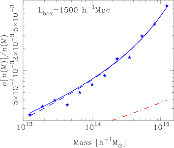
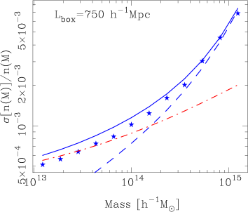
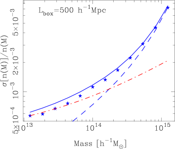
Figure 3 presents the fractional errors on the mass function, , from both theory and simulations, for the subcube sizes mentioned in §5.3. In all panels the points denote the measurements from the simulations. The theoretical predictions of Eq. (25), are estimated for a single realization of given size , following the recipe at the end of §5.2. Then the variance is rescaled by , so that the fractional errors in all four panels correspond to a total volume of .
The agreement between the theory and the measurements is very good, with a slight difference at the low-mass end for the subcubes considered. This difference does not occur when the estimate is made using the full simulation boxes to estimate the variance (see top left panel of Figure 3). We also note that the Poisson model (dashed lines) agrees well with the simulations at the high-mass end. However, at lower masses, the variance becomes dominated by the sample variance, as given by the first term of Eq. (25). For a mass bin the latter is simply:
| (47) |
and this is denoted in Figure 3 by the dot-dashed lines.
On comparing all four panels, we observe that with the exception of the first panel with , the results are almost indistinguishable. This is quite interesting, since for these subcube volumes, Fig. 1 shows to be a decreasing function of . For a given mass bin we would expect the errors for the smaller subcube measurements to be significantly larger. This is indeed the case, but the fact that we use the variance on the mean, i.e. we divide by , leads to results that are very similar.
The slight difference between the measurements and the predictions is not easy to understand, since for the theoretical estimation we use measured from the simulations. This is done for all subcubes, so we do take into account that modes with wavelength larger than the subcube size may contribute to the covariance in the subcubes. The limit is set by the size of the original simulation box . However, the bias is the Sheth-Tormen prescription, which Figure 2 shows to be slightly lower than the one measured from the halo-halo power spectrum. This effect might be more pronounced for the small-mass bins, but more work is needed here to arrive to a definitive conclusion, and we defer this to a future study.
Before moving on, we note that this startling agreement for the fractional errors on the mass function was noted before by Crocce et al. (2010). In that work the variance on a given subcube scale was computed theoretically using the linear theory variance in a spherical top-hat taken to have the same volume as the subcube (see earlier discussion in §3). These authors pointed out that when using an ensemble of simulations with no subcubing the theory over-predicted the measurements. Here we have shown that there is no conflict between the theory and the measurements, if one uses the volume variance measured from the simulations.
5.5. Measurements: covariance
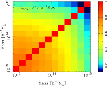
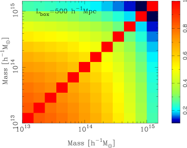
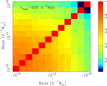
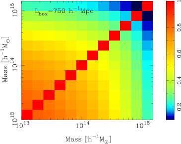
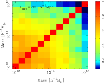
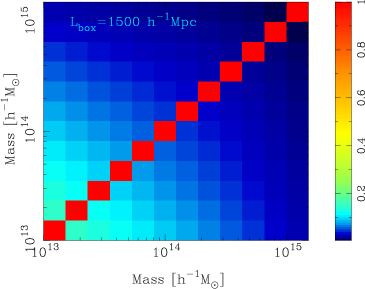
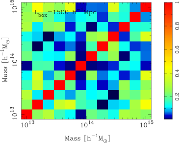
Figure 4 presents the theoretical mass function correlation matrix from Eq. (29) versus the measured one. The left panels show the predictions, obtained in the same way as in Figure 3, and the right ones the measurements. From top to bottom, the following subcube sizes are considered: .
The figure reveals a remarkable agreement between measurements and theory: the trend observed in Figure 3 is also present here, with the predictions marginally larger than the measurements in some of the mass bins. We find that the measurements are strongly covariant: for clusters with , the cross-correlation coefficeint is . Only for the highest-mass clusters does the covariance matrix become close to diagonal. The exception is for the ensemble of cubes with . In this case the realizations appear to be only weakly correlated with , for . However, as was discussed above and shown in Figure 1, the behaviour of at the simulation box scale is not representative for the real Universe, owing to the absence of power on larger scales. Had we run a simulation of larger volume, then the volume variance on the scale would have been significantly larger.
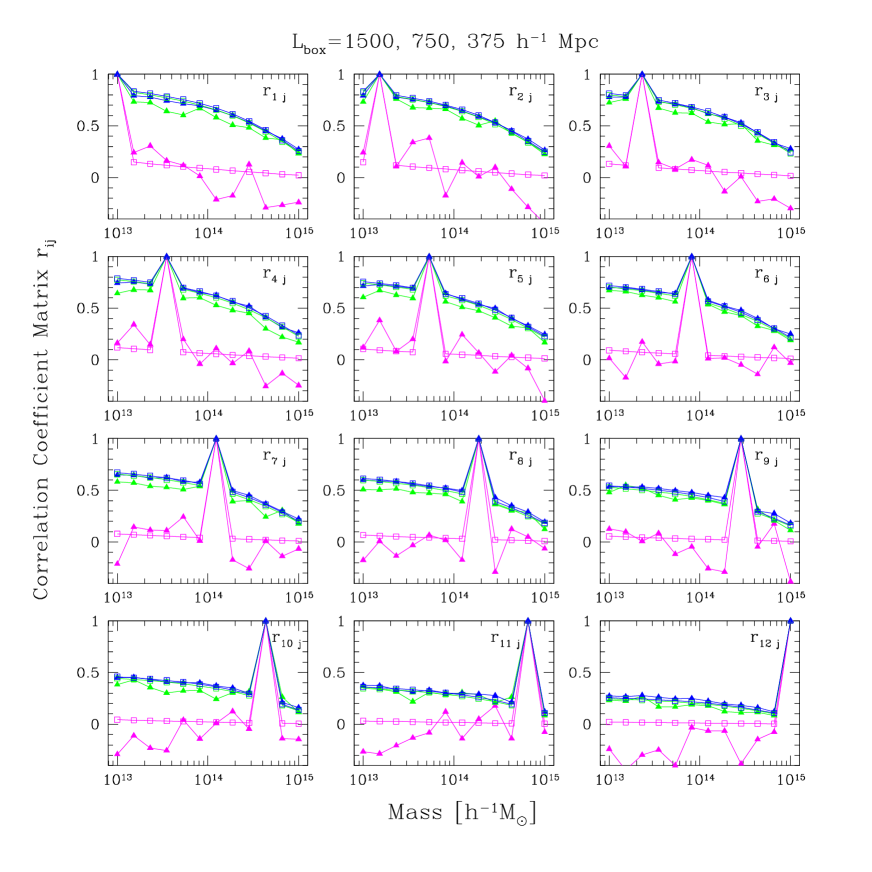
Figure 5 presents the same information as Figure 4, but in a more quantitative format. The plot has 12 panels, with each panel depicting a single row from the correlation matrix, i.e. vs , with fixed. In this plot the solid triangles denote the measured correlation coefficient, while the empty squares represent the theory predictions. For clarity, we show results only for the box sizes , represented by the magenta, green, and blue symbols respectively. It is clear from this figure too that the theory predictions and the measurements are in remakably good agreement. On comparing the correlation coefficient for different subcube sizes, we again note the similarity of these results, despite the variation in : just as in Fig. 3, the covariance on the mean leads to the observed similarity. The exception is for the cubes, and we offer the same explantion for this as noted above.
We conclude this section by stating that Eq. (25) gives a very reliable prediction for the mass function covariance, provided one employs the true variance within the volume.
6. Cosmological information from the mass function
In this section we examine how the cosmological information content of the cluster mass function changes, when we exchange the standard Poisson assumption for the more complex likelihood models of Eqs (10) and (14).
6.1. Fisher information
In all cases we shall use the standard definition of the Fisher information (for an excellent review of Fisher matrix techniques in cosmology see Heavens, 2009):
| (48) |
where and are elements of the cosmological model parameter set upon which the likelihood depends. From the Fisher matrix, one may obtain an estimate of the marginalized errors and covariances of the parameters:
| (49) |
as well as the unmarginalized errors:
| (50) |
6.2. The Poisson Fisher matrix
In the case of Poisson errors for each cell and mass bin, then using Eqs (2) and (13) we write:
| (51) | |||||
On partially differentiating the above expression with respect to parameters and then , and on performing the ensemble average, one finds:
| (52) |
6.3. The Gaussian Fisher matrix
As was shown earlier, in the case of the full likelihood model for the counts (c.f. Eq. (10)), we expect the Fisher matrix to be significantly modified from the Poisson case in the region of many counts per mass bin. In this limit, the likelihood is given by Eq. (14), and we have the standard result for the Fisher information for a Gaussian likelihood (Tegmark et al., 1997):
| (53) |
6.4. The Gauss-Poisson Fisher matrix
LH04 developed an approximation for the Fisher matrix, which interpolates between the correct forms for the information in the limit of rare peaks and sample-variance-dominated counts. Their expression is:
| (54) |
where , and is a diagonal matrix with the elements , as defined in §2.
6.5. Estimating Fisher matrices from simulations
In order to evaluate all of the expressions for the Fisher matrices presented in the previous sections, we require knowledge of three quantities: the partial derivatives of the mean counts with respect to the parameters ; the inverse of the total covariance matrix ; and the derivative of the sample variance covariance matrix . In this section we shall use numerical simulations to directly evaluate all of these quantities.
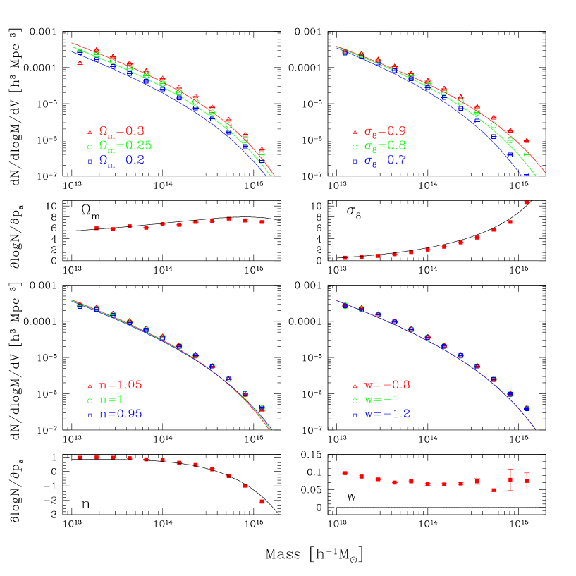
We first measure the halo mass function for each of the variational cosmologies described in §4. With this information we are then able to numerically obtain the derivatives for the simulated parameters . When computing the mass function derivatives, we reduce the effects of cosmic variance on the estimates, using the fact that the first 4 simulations of the fiducial cosmology have matched initial conditions with the 4 variational-cosmologies simulations. Hence, our reduced-cosmic-variance estimator for the derivatives can be written:
| (55) |
where is the average mass function for mass bin , estimated from all 40 independent realizations; is the number of the variational simulations; denotes the simulation realization going from to ; is the mass function in the fiducial case, estimated for each of the 4 realizations that have matched initial conditions to the variational-cosmologies realizations (for an explict defintion of this see Eq. (B1)). The logarithmic derivatives are estimated as:
| (56) |
Note that since we estimate using double-sided derivatives, we may take larger step sizes in the parameters to compute the derivatives than would be allowed for single sided derivatives (Eisenstein et al., 1999). For the former case, the errors in the derivatives are of quadratic order in the step size: i.e. . Thus parameter step sizes of 20% and 10% should correspond to relative errors of roughly 4% and 1% in the derivatives, respectively. In actuallity, the true accuracy of the derivatives also depends on the value of the third partial derivative.
In Figure 6 we show simulation measurements of the average mass functions for the fiducial and variational cosmologies. This figure makes very clear not only the sensitivity of the mass function to the cosmological parameters considered, but also the halo mass range over which most of it occurs. Changes in and the slope of the primordial power spectrum impact the mass function for the whole range of halo masses. The low-mass end is less sensitive to variations in , while the dark energy equation of state parameter barely affects the mass function.
In the smaller panels of Figure 6 we show the derivatives of the halo abundance, estimated using Eq. (56). The error bars are computed as errors on the mean of the realizations, as they are also for the mass functions in the larger panels. The -derivative is almost constant and large for all bins, while the one monotonically increases from 0 at the low mass end to a large value at the high mass end. The behaviour of the spectral-index-derivative is quite interesting, as it changes sign at and becomes negative at the high mass end. Its overall variation is not as large as in the case of and , which will be better constrained by the halo abundance.
Another interesting finding of this exploration concerns the -derivative, which should be at redshift according to linear theory and the Sheth-Tormen mass function. We find it to be small and positive, , for most of the mass range considered, and rising slightly to at the low-mass end. The -derivative does not vanish because in reality the mass function depends on the full nonlinear growth history. This encompasses the growth of structure at all redshifts, and thus makes the present day halo abundance sensitive to . These results are consistent with the findings in earlier studies (Linder & Jenkins, 2003; Jennings et al., 2010).
We next follow the recipe of §5.3, to estimate the covariance matrices in each of the variational cosmological models. From these estimates we are then able to form the partial derivatives of the covariance with respect to the cosmological parameters: . Again, as was done for , we take advantage of the matched intial conditions to reduce the cosmic variance on the estimates of the partial derivatives of the covariance matrix.
6.6. Forecasted errors
Having obtained all of the necessary ingredients we are now in a position to evaluate the Fisher information directly from the simulations.
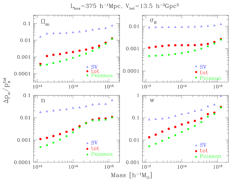
Figure 7 shows the cumulative fractional Fisher errors, , estimated using Eq. (50), as a function of the minimum cluster mass, and for the four cosmological parameters that we consider. The results obtained for the various subcube sizes are almost identical with the exception of the case where : as explained earlier, the underestimate of the variance on scales of the simulation makes the estimate of the mass function covariance, and hence the Fisher errors unrealistic. For brevity we shall present only the findings for , which we consider very reliable.
For our fiducial survey, we adopt parameters relevant for future all-sky -ray cluster surveys, such as eROSITA (Predehl et al, 2010). This mission will be able to target intermediate mass range clusters, and not just the most massive objects in the Universe as is the case for current and past surveys. We adopt a total survey volume of , and we rescale our measured covariance matrices to this volume. For this comoving volume at , we find in the simulations approximately halos in the mass interval , halos in the interval , halos in the interval , and 8000 halos with masses larger than the latter limit.
In Fig. 7 the solid green squares denote the results obtained for the Poisson Fisher matrix, as given by Eq. (52). The solid red circles denote the errors resulting from the second term of Eq. (54). The blue triangular-shaped symbols denote the errors obtained from only the trace-part of Eq. (54), where instead of , we have used the covariance matrix from our simulations (c.f. Eq. (46)). We do not expect that replacing with will change our conclusions concerning the information carried by this term, except to possibly make the errors larger.
As expected, for all of the cosmological parameters considered, the fractional errors obtained from the Poisson approximation are smallest. Including the full covariance matrix, as in the second term of Eq. (54), reduces the amount of information, and this results in a significant increase in the fractional errors. For the case of , the errors are roughly a factor of 3 larger when the full-covariance is used as opposed to the Poisson case. When , the errors are only a factor of 2 worse. For the rarest objects, where the covariance becomes almost diagonal, the errors from the two methods are very similar. We find that the trace part of Eq. (54) contributes negligibly to the information, and if this term is taken separately, it yields errors that are roughly one order of magnitude larger than those from the second term.
Let us explore the consequences of this last result a little further. Consider the Fisher matrix given by Eq. (54), if the first term on the right-hand-side is negligable, then the information about each cosmological parameter enters the system only through the derivatives of the model mean with respect to the parameters. Since the model here is the mean counts, the bias provides no information. However, the amplitude of the elements of the information matrix can be modulted by the inverse covariance matrix. Owing to the fact that increasing the elements of the covariance matrix only leads to a smaller inverse covariance, we thus conclude that, adding the variance from the bias can only ever decrease the Fisher information. However, as discussed in Lima & Hu (2005), the information content of the first term of Eq. (54), becomes of great importance in the presence of a scatter between the true and observed mass.
Note also that the cumulative dependence of the errors on the mass bins, can partly be understood by examining the behaviour of the derivatives as shown in Fig. 6. The errors flatten out at those points in the mass range where the derivatives of the parameters are close to 0, as in the case of at the low-mass end, or at masses .
Finally, we emphasize that the forecasts that we make above are to illustrate the importance of going beyond the Possion likelihood approximation and should not be taken as serious predictions for a potential survey. The cosmological dependence that we have considered here arises strictly from the mass function. In order to make a realistic forecast we would have to take into account a number of observational factors: realistic survey geometries; the evolution of the mass function with redshift; the evolution of the volume element with the cosmological model; and the evolution in the minimum detectable mass at each redshift; and a scatter in the relation between the observed mass proxy and the true cluster mass (see Marian & Bernstein, 2006, for an example of forecasting weak lensing cluster counts.).
7. Summary and conclusions
In this paper, we have studied the covariance of the halo mass function, and the cosmological information content of such data. We adopted a two-line attack on these problems: the first line was theoretical and we developed an analytic model to explore these issues; the second was the use of a large ensemble of numerical simulations to measure directly all quantities of interest.
In §2, we summarized the counts-in-cells formalism (Peebles, 1980; Hu & Kravtsov, 2003), and developed it for application to deal with cluster counts in multiple mass bins. We described the Gauss-Poisson likelihood function for the counts in cells with multiple mass bins. The expression was analogous to that derived by Lima & Hu (2004) for multiple cells and a single mass bin.
In §3, we used this framework to derive a formal expression for the covariance of the halo mass function and the cross-correlation coefficient, i.e. Eqs (25) and (29), respectively. We found that there were two terms contributing: a Poisson shot-noise term, which dominates in the limit of rare clusters; and a term associated with the sample variance, which is dominant for abundant clusters. This expression is analogous to the results of Hu & Kravtsov (2003) for multiple cells and a single mass bin. The expression was found to depend on three quantities: the cluster mass function; the cluster bias; and the variance in the survey volume.
In §4, we presented the details of our large ensemble of numerical simulations: 40 simulations of a fiducial model and 32 simulations of modified cosmological models.
In §5, we made a rigorous comparison of the results from the theoretical modelling with those obtained directly from the numerical simulations. We measured the variance of matter and cluster fluctuations in cells of various sizes and found, for spherical and cubical top-hat cells, that the simulations and theory predictions were discrepant for large cell sizes. We showed that this was entirely attributable to the difference between the discrete lattice structure of the Fourier space in the simulations, and the continuum of Fourier modes in the theory integrals. The cubical and spherical top-hat simulation results were in good agreement, except on the largest scales where simulation box-scale effects were important.
We also measured the halo bias in cells of various sizes from the simulations. We found that the bias from the halo-mass cross-variance showed very little scale dependence over the range , whereas that from the halo auto-variance showed significant scale dependence, before and after the shot-noise correction. We found that the Sheth & Tormen (1999) model was an excellent fit to the former and a reasonable fit to the latter.
We then measured the covariance of the mass function in the simulations. To increase the number of realizations, we used the strategy of subdividing each large simulation volume into a set of smaller subcubes. We found that the estimated covariances were in excellent agreement with the theoretical predictions. This was under the condition that we used the actual variance of mass fluctuations measured in the simulations.
In §6, we employed the Fisher matrix formalism to explore the information content of the cluster counts. Using the more realistic likelihood functions, we demonstrated numerically that the Poisson likelihood model only provides a reasonably accurate description of the data for clusters that are more massive than . Future surveys that aim to target cluster samples with masses , must adopt more sophisticated likelihood analysis, such as discussed by Lima & Hu (2004), Hu & Cohn (2006) and here in, which take into account the full covariance matrix of the counts. Otherwise, significant underestimates of the true errors will occur.
There are a number of possible future directions for the work that we have presented here. Firstly, as pointed out by Lima & Hu (2005), one of the main uses of adopting the counts-in-cells approach is that it helps to lift the degeneracy between nuisance parameters, which are involved in calibrating the cluster masses, and the cosmological parameters. This occurs beacuse the sample varaince depends on the bias of the clusters, which has a different behaviour with cosmological parameters than the counts. Whilst we have shown explicitly that the terms in the Fisher matrix that depend on the derivatives of the covariance matrix, and hence derivatives of the bias, do not carry a great deal of cosmological information by themselves, it will be interesting to see whether for a more realistic scenario, where one must marginalize over these nuisance parameters, the self-calibration can be successfully performed to restore the lost information.
We also note that the counts-in-cells technique has been highlighted as a powerful means for constraining primordial non-Gaussianity (Oguri, 2009; Cunha et al., 2010; Marian et al., 2011). It is of some importance to explore this approach using numerical simulations, since it is not clear whether the extension of the current formalism to such modified cosmological models works in practice.
Acknowledgements
We thank Gary Bernstein and Ravi Sheth for comments on the draft and Raul Angulo, Martin Crocce, Peter Schneider, Uros Seljak and Yu-Ying Zhang for useful discussions. We thank V. Springel for making public GADGET-2 and for providing his B-FoF halo finder, and R. Scoccimarro for making public his 2LPT code. RES acknowledges support from a Marie Curie Reintegration Grant, an award for Experienced Researchers from the Alexander von Humboldt Foundation and partial support from the Swiss National Foundation under contract 200021-116696/1. LM is supported by the Deutsche Forschungsgemeinschaft through the grant MA4967/1-1.
References
- Abate et al. (2009) Abate, A., Wittman, D., Margoniner, V. E., Bridle, S. L., Gee, P., Tyson, J. A., & Dell’Antonio, I. P. 2009, ApJ, 702, 603
- Albrecht et al. (2006) Albrecht, A., Bernstein, G., Cahn, R., Freedman, W. L., Hewitt, J., Hu, W., Huth, J., Kamionkowski, M., Kolb, E. W., Knox, L., Mather, J. C., Staggs, S., & Suntzeff, N. B. 2006, ArXiv Astrophysics e-prints
- Allen et al. (2003) Allen, S. W., Schmidt, R. W., Fabian, A. C., & Ebeling, H. 2003, MNRAS, 342, 287
- Borgani et al. (2001) Borgani, S., Rosati, P., Tozzi, P., Stanford, S. A., Eisenhardt, P. R., Lidman, C., Holden, B., Della Ceca, R., Norman, C., & Squires, G. 2001, ApJ, 561, 13
- Cole & Kaiser (1989) Cole, S. & Kaiser, N. 1989, MNRAS, 237, 1127
- Crocce et al. (2010) Crocce, M., Fosalba, P., Castander, F. J., & Gaztañaga, E. 2010, MNRAS, 403, 1353
- Crocce et al. (2006) Crocce, M., Pueblas, S., & Scoccimarro, R. 2006, MNRAS, 373, 369
- Cunha et al. (2010) Cunha, C., Huterer, D., & Doré, O. 2010, PRD, 82, 023004
- Davis et al. (1985) Davis, M., Efstathiou, G., Frenk, C. S., & White, S. D. M. 1985, ApJ, 292, 371
- DES (2005) DES. 2005, ArXiv Astrophysics e-prints
- Eisenstein et al. (1999) Eisenstein, D. J., Hu, W., & Tegmark, M. 1999, ApJ, 518, 2
- Gladders et al. (2007) Gladders, M. D., Yee, H. K. C., Majumdar, S., Barrientos, L. F., Hoekstra, H., Hall, P. B., & Infante, L. 2007, ApJ, 655, 128
- Heavens (2009) Heavens, A. 2009, ArXiv e-prints
- Henry (2004) Henry, J. P. 2004, ApJ, 609, 603
- Hu & Cohn (2006) Hu, W. & Cohn, J. D. 2006, PRD, 73, 067301
- Hu & Kravtsov (2003) Hu, W. & Kravtsov, A. V. 2003, ApJ, 584, 702
- Israel et al. (2010) Israel, H., Erben, T., Reiprich, T. H., Vikhlinin, A., Hildebrandt, H., Hudson, D. S., McLeod, B. A., Sarazin, C. L., Schneider, P., & Zhang, Y. 2010, A&A, 520, A58+
- Jennings et al. (2010) Jennings, E., Baugh, C. M., Angulo, R. E., & Pascoli, S. 2010, MNRAS, 401, 2181
- Komatsu et al. (2010) Komatsu, E., , & The WMAP Team. 2010, ArXiv e-prints
- Komatsu et al. (2009) Komatsu, E., Dunkley, J., Nolta, M. R., Bennett, C. L., Gold, B., Hinshaw, G., Jarosik, N., Larson, D., Limon, M., Page, L., Spergel, D. N., Halpern, M., Hill, R. S., Kogut, A., Meyer, S. S., Tucker, G. S., Weiland, J. L., Wollack, E., & Wright, E. L. 2009, ApJS, 180, 330
- Lima & Hu (2004) Lima, M. & Hu, W. 2004, PRD, 70, 043504
- Lima & Hu (2005) —. 2005, PRD, 72, 043006
- Linder & Jenkins (2003) Linder, E. V. & Jenkins, A. 2003, MNRAS, 346, 573
- LSST (2009) LSST. 2009, ArXiv e-prints
- Manera & Mota (2006) Manera, M. & Mota, D. F. 2006, MNRAS, 371, 1373
- Mantz et al. (2008) Mantz, A., Allen, S. W., Ebeling, H., & Rapetti, D. 2008, MNRAS, 387, 1179
- Mantz et al. (2010) Mantz, A., Allen, S. W., Rapetti, D., & Ebeling, H. 2010, MNRAS, 406, 1759
- Marian & Bernstein (2006) Marian, L. & Bernstein, G. M. 2006, PRD, 73, 123525
- Marian et al. (2011) Marian, L., Hilbert, S., Smith, R. E., Schneider, P., & Desjacques, V. 2011, ApJL, 728, L13+
- Mo & White (1996) Mo, H. J. & White, S. D. M. 1996, MNRAS, 282, 347
- Muchovej et al. (2011) Muchovej, S., Leitch, E., Carlstrom, J. E., Culverhouse, T., Greer, C., Hawkins, D., Hennessy, R., Joy, M., Lamb, J., Loh, M., Marrone, D. P., Miller, A., Mroczkowski, T., Pryke, C., Sharp, M., & Woody, D. 2011, ApJ, 732, 28
- Oguri (2009) Oguri, M. 2009, Physical Review Letters, 102, 211301
- Okabe et al. (2010) Okabe, N., Zhang, Y.-Y., Finoguenov, A., Takada, M., Smith, G. P., Umetsu, K., & Futamase, T. 2010, ApJ, 721, 875
- Peebles (1980) Peebles, P. J. E. 1980, The large-scale structure of the universe (Research supported by the National Science Foundation. Princeton, N.J., Princeton University Press, 1980. 435 p.)
- Planck Collaboration et al. (2011) Planck Collaboration, Ade, P. A. R., Aghanim, N., Arnaud, M., Ashdown, M., Aumont, J., Baccigalupi, C., Balbi, A., Banday, A. J., Barreiro, R. B., & et al. 2011, ArXiv e-prints
- Predehl et al (2010) Predehl et al. 2010, in Society of Photo-Optical Instrumentation Engineers (SPIE) Conference Series, Vol. 7732, Society of Photo-Optical Instrumentation Engineers (SPIE) Conference Series
- Press & Schechter (1974) Press, W. H. & Schechter, P. 1974, ApJ, 187, 425
- Press et al. (1992) Press, W. H., Teukolsky, S. A., Vetterling, W. T., & Flannery, B. P. 1992, Numerical recipes in FORTRAN. The art of scientific computing (Cambridge: University Press, —c1992, 2nd ed.)
- Refregier et al. (2010) Refregier, A., Amara, A., Kitching, T. D., Rassat, A., Scaramella, R., Weller, J., & Euclid Imaging Consortium, f. t. 2010, ArXiv e-prints
- Reiprich & Böhringer (2002) Reiprich, T. H. & Böhringer, H. 2002, ApJ, 567, 716
- Rozo et al. (2010) Rozo, E., Wechsler, R. H., Rykoff, E. S., Annis, J. T., Becker, M. R., Evrard, A. E., Frieman, J. A., Hansen, S. M., Hao, J., Johnston, D. E., Koester, B. P., McKay, T. A., Sheldon, E. S., & Weinberg, D. H. 2010, ApJ, 708, 645
- Schirmer et al. (2007) Schirmer, M., Erben, T., Hetterscheidt, M., & Schneider, P. 2007, A&A, 462, 875
- Schuecker et al. (2003) Schuecker, P., Böhringer, H., Collins, C. A., & Guzzo, L. 2003, A&A, 398, 867
- Scoccimarro (1998) Scoccimarro, R. 1998, MNRAS, 299, 1097
- Sehgal & The ACT Collaboration (2011) Sehgal, N. & The ACT Collaboration. 2011, ApJ, 732, 44
- Seljak et al. (2003) Seljak, U., Sugiyama, N., White, M., & Zaldarriaga, M. 2003, PRD, 68, 083507
- Seljak & Zaldarriaga (1996) Seljak, U. & Zaldarriaga, M. 1996, ApJ, 469, 437
- Sheth & Tormen (1999) Sheth, R. K. & Tormen, G. 1999, MNRAS, 308, 119
- Sheth & Tormen (2002) —. 2002, MNRAS, 329, 61
- Sirko (2005) Sirko, E. 2005, ApJ, 634, 728
- Smith et al. (2003) Smith, R. E., Peacock, J. A., Jenkins, A., White, S. D. M., Frenk, C. S., Pearce, F. R., Thomas, P. A., Efstathiou, G., & Couchman, H. M. P. 2003, MNRAS, 341, 1311
- Smith et al. (2007) Smith, R. E., Scoccimarro, R., & Sheth, R. K. 2007, PRD, 75, 063512
- Springel (2005) Springel, V. 2005, MNRAS, 364, 1105
- Sunyaev & Zeldovich (1972) Sunyaev, R. A. & Zeldovich, Y. B. 1972, Comments on Astrophysics and Space Physics, 4, 173
- Tegmark et al. (1997) Tegmark, M., Taylor, A. N., & Heavens, A. F. 1997, ApJ, 480, 22
- Valageas et al. (2011) Valageas, P., Clerc, N., Pacaud, F., & Pierre, M. 2011, ArXiv e-prints
- Vanderlinde & The SPT Collaboration (2010) Vanderlinde, K. & The SPT Collaboration. 2010, ApJ, 722, 1180
- Vikhlinin et al. (2009) Vikhlinin, A., Kravtsov, A. V., Burenin, R. A., Ebeling, H., Forman, W. R., Hornstrup, A., Jones, C., Murray, S. S., Nagai, D., Quintana, H., & Voevodkin, A. 2009, ApJ, 692, 1060
- Wang & Steinhardt (1998) Wang, L. & Steinhardt, P. J. 1998, ApJ, 508, 483
- Zhang et al. (2007) Zhang, Y.-Y., Finoguenov, A., Böhringer, H., Kneib, J.-P., Smith, G. P., Czoske, O., & Soucail, G. 2007, A&A, 467, 437
- Zhang et al. (2008) Zhang, Y.-Y., Finoguenov, A., Böhringer, H., Kneib, J.-P., Smith, G. P., Kneissl, R., Okabe, N., & Dahle, H. 2008, A&A, 482, 451
Appendix A The volume variance
In this section we investigate the impact of systematic effects on the volume variance, which arise due to the anisotropic lattice in Fourier space and also low- and high- truncation of the matter power spectrum.
A.1. Fourier lattice versus a continuum of modes
As was described in §3.4 the matter variance in the volume is a key quantity for correctly evaluating the covariance matrix of the cluster counts. Also, as was shown in §5.1, there is a discrepancy between the theoretical predictions and meaurements in simulations obtained for . We now investigate the origin of these discrepancys.
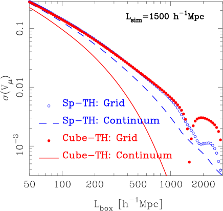
We start by examining the importance of the discrete cubical Fourier lattice, which is used in the estimates from the simulations, and the continuum of Fourier modes, which is used to evaluate the theory. We start by generating a Fourier lattice as in the simulations, where each lattice point is spaced from the next one, along each dimension, by . Then at each lattice point, we compute the magnitude of the -vector and evaluate the linear theory power spectrum at that point. is then obtained as described in Eq. (40), by summing up the grid of power spectra values multiplied by the square of the appropriate window function. The top panel of Figure 8 shows the results of this exercise for both the spherical and cubical window functions. We also compare this to the results obtained from the theory, assuming a continuum of modes. The results that we find for the theory evaluated on the cubical mesh, are in remarkably good agreement with the measurements from the simulations presented in Fig. 1.
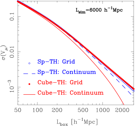
To be sure that the discrepancy is due to the lattice, we should expect that as the simulation box size becomes significantly larger, the results for the lattice should approach those of the continuum. We test this by regenerating the Fourier lattice, but this time taking , and keeping the maximum Fourier mode the same as before. The results of this exercise are shown in the bottom panel of Fig. 8. We clearly see that the results are now in much better agreement and for the same cell sizes as in the upper panel.
Thus we are led to conclude that in matching the results from the simulations we must be mindful to take into account the anisotropic lattice structure of the Fourier space to obtain accurate comparisons between the theory and the simulations. This then further justifies our choice of using the measured in the simulations to make the predictions for the covariance of the counts.
Finally, these results also act as a cauationary tale: when interpreting the results of numerical simulations on very large scales, we should take more care in asigning the power to the lattice cells in the initial conditions. We should use methods that supress this discretization. For instance, it would seem more sensible to compute the power averaged over a lattice cell and not simply the power at the lattice cell point. Also including the missing zero modes may be a more realistic stratergy (see for example Sirko, 2005).
A.2. Cut-off scales
In Figure 1 we evaluated the integrals in Eqs (34) and (38), keeping the upper and lower bounds fixed at the values and . This was done for a fair comparison with our simulations, which do not have modes larger than the simulation box , nor structures smaller than the softening scale, . We now present a short discussion of how the mass-fluctuations-variance depends on the cell volume and the cut-off scales in the power spectrum.
For the large cell sizes that we are interested in, i.e. , we find no dependence of on , for the range of values .
For the lower cut-off scale , the situation appears to be more complex. In Figure 9, we show the result of computing the mass-fluctuations-variance averaged in cubical and spherical top-hat volumes, as a function of the cubical cell volume (recall that we take the radius of the spherical top-hat cell to be ). In the plot we consider the values of for three different simulation sizes: . These box sizes correspond to the: solid red, long-dashed green, and dot-dashed magenta lines, respectively. The thicker/thinner lines in the plot depict the spherical/cubical top-hat smoothing.
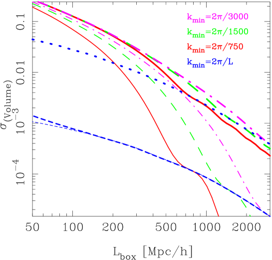
For the case of the spherical top-hat filter, we find that the variance for , is roughly a factor of 2 times smaller than the variance obtained when . However, for the case of the cubical top-hat window function, we find that the difference in the variance for these same two values of , is more than an order of magnitude.
In Figure 9, the thick dotted blue curve presents predictions for with the spherical window function, but where we now take the lower limit . The thick and thin dashed blue lines show the same, but for the case of the cubical filter function. For this case, the thin line is obtained when the linear theory matter power spectrum is used, and the thicker line shows the results obtained when the nonlinear power spectrum from halofit (Smith et al., 2003) is employed. The differences are very small. Thus using the linear theory power spectrum for the mass variance is quite reasonable on these scales. The main point of this last example, is to show that for large cell sizes, the results for are very sensitive to the presence/absence of power on very large scales.
Appendix B Convergence of the covariance matrix
B.1. Covariances from individual simulations
Here we consider an alternate approach to estimating the covariance of the cluster counts. We are concerned that, if there is a significant variance of the cluster counts on the scales of the simulation cube, then by computing the covariance around the mean cluster mass function averaged over all simulations, we are overestimating the covariance. To anwer this question, we adopt the stratergy of using the sub-cubes in a single simulation to make an estimate of the covariance, and finally we then average these estimates over all the simulations.
For each simulation run we therefore have:
| (B1) |
where is the number of counts in the run, subcube and mass bin. The covariance for each run is:
| (B2) | |||||
and the average covariance:
| (B3) |
We have checked that using Eqs (B1) and (B2) does not change the measured mass function covariance in any significant way. We therefore conclude that the method of estimating the covariance described in §5.3, is not biased by the estimates of the mean density.
B.2. The chessboard test
When dividing a big simulation box into smaller subcubes, the largest wavelength modes may affect the observables measured in the smaller cubes. In the case of clusters, some of the subcubes may have very different mean counts than others, and in general, the smaller the sub-boxes, the larger the expected covariance between them. This is also true for real surveys, which measure observables in a finite volume of the Universe: some of these observables are impacted by modes larger than the size of the survey.
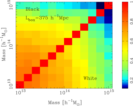
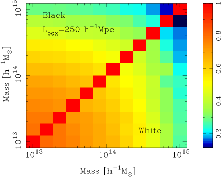
In order to check the validity of our approach, we measure the covariance of the mass function using subcubes that are not adjacent, and should therefore be less covariant. We shall refer to this as the ‘chessboard test’, as its 2D analogue would be similar to using only the white or the black squares of a chessboard to compute the mass function covariance. This test has the limitation that large mode correlations can span more than just 2 subcubes, particularly if the latter are small. Nevertheless, if we find the covariance measured from the ‘white’ subcubes different from that obtained from the ‘black’ ones and also different from the all-subcubes-covariance, then our box-division method is flawed.
We perform this test for the conservative values , i.e. we consider and subcubes, with volumes and , respectively. The result is shown in Figure 10. There is no major difference between the ‘white’, ‘black’, and total mass function correlation matrix (c.f. Fig. 4). We conclude that modes with wavelengths smaller than the size of the subcubes considered here, are not explicitly responsible for generating the mass function covariance.
