Comprehensive study of the critical behavior in the diluted antiferromagnet in a field

Abstract

We study the critical behavior of the Diluted Antiferromagnet in a Field with the Tethered Monte Carlo formalism. We compute the critical exponents (including the elusive hyperscaling violations exponent $\theta$). Our results provide a comprehensive description of the phase transition and clarify the inconsistencies between previous experimental and theoretical work. To do so, our method addresses the usual problems of numerical work (large tunneling barriers and self-averaging violations).

Understanding collective behavior in the presence of quenched disorder has long been one of the most challenging and interesting problems in statistical mechanics. One of its simplest representatives is the random field Ising model (RFIM), which has been extensively studied both theoretically and experimentally.Nattermann (1998); *belanger:97 The RFIM is physically realized by a diluted antiferromagnet in an applied magnetic field (DAFF).

It is known that the $D=3$ DAFF/RFIM undergoes a phase transition, but the details remain controversial, with severe inconsistencies between analytical, experimental and numerical work. A scaling theory is generally accepted, where the dimension $D$ of the system is replaced by $D-\theta$ in the hyperscaling relation. This third independent critical exponent, believed to be $\theta\approx 1.5$, is inaccessible both to a direct experimental measurement and to traditional Monte Carlo methods.

The values of the remaining critical exponents, seemingly more straightforward, are also controversial. On the experimental front, different ansätze for the scattering line shape yield mutually incompatible estimates of the thermal critical exponent, namely $\nu=0.87(7)$ (Ref. Slanic et al., 1999), or $\nu=1.20(5)$ (Ref. Ye et al., 2004). Furthermore, the experimental estimate of the anomalous dimension, $\eta=0.16(6)$ (Ref. Slanic et al., 1999), violates hyperscaling bounds, if one is to believe the experimental claims of a diverging specific heat ($\alpha\geq 0$). Belanger et al. (1983); *belanger:98

On the other hand, the numerical determination of $\nu$ has steadily shifted, the most precise estimate being $1.37(9)$ (Ref. Middleton and Fisher, 2002), inconsistent with the experimental values and barely compatible with $\alpha\approx 0$. The value of $\alpha$ itself is very hard to measure in a numerical simulation. Hartmann and Young (2001); *malakis:06

More fundamentally, the smallness of the magnetic exponent $\beta$, combined with the numerical observation of metastability, Sourlas (1999); *wu:06; *maiorano:07 has led some authors to suggest that the transition in the DAFF may be of first order.

Ultimately, the physical reasons for this confusion betray the fact that the traditional tools of statistical mechanics are ill-suited to systems with rugged free-energy landscapes. Both experimentally and numerically, the system gets trapped in local minima, with escape times that grow as $\log\tau\sim\xi^{\theta}$ ($\xi$ is the correlation length). This not only makes it exceedingly hard to thermalize the system, but also generates a rare-events statistics, causing self-averaging violations. Parisi and Sourlas (2002); *fytas:11

In this letter we study the DAFF with the Tethered Monte Carlo (TMC) formalism. Fernandez et al. (2009) Our approach restores self-averaging and is able to negotiate the free-energy barriers of the DAFF to equilibrate large systems safely. It also provides direct access to the key parameter $\theta$. We thus obtain a comprehensive picture of the phase transition, consistent both with analytical results for the RFIM and with experiments on the DAFF, and shed light on the reasons behind the previous discrepancies.

In the following we provide a brief outline of the tethered formalism applied to the DAFF (see Refs. Fernandez et al., 2009; Martin-Mayor et al., 2011 for details). We note, however, that we give most of our physical results translated into the familiar canonical language. In a tethered computation, we run simulations where one (or more) order parameters of the system are (almost) constrained. In this way, we eliminate the need for exponentially slow tunneling caused by the free-energy barriers associated to these parameters. From these tethered simulations the Helmholtz effective potential is accurately reconstructed with a fluctuation-dissipation formalism.

We consider a system with $N=L^{D}$ spins, $s_{\boldsymbol{x}}=\pm 1$, on the nodes of a cubic lattice with periodic boundary conditions and interacting through the Hamiltonian

$$H=\sum_{\langle{\boldsymbol{x}},{\boldsymbol{y}}\rangle}\epsilon_{\boldsymbol{x}}s_{\boldsymbol{x}}\epsilon_{\boldsymbol{y}}s_{\boldsymbol{y}}-hM-h_{\text{s}}M_{\text{s}}=U-hM-h_{\text{s}}M_{\text{s}}.$$ (1)

Here $h$ and $h_{\text{s}}$ are the applied fields, coupled to the magnetization and staggered magnetization,

$$M =Nm=\sum_{\boldsymbol{x}}\epsilon_{\boldsymbol{x}}s_{\boldsymbol{x}}, M_{\text{s}} =\sum_{\boldsymbol{x}}\epsilon_{\boldsymbol{x}}s_{\boldsymbol{x}}\mathrm{e}^{\mathrm{i}\pi\sum_{\mu=1}^{D}x_{\mu}}.$$ (2)

We are ultimately interested in $h_{\text{s}}=0$, but we will find this parameter useful. The quenched occupation variables $\epsilon_{\boldsymbol{x}}$ are $1$ with probability $p=0.7$ and zero otherwise (this value is chosen to be far both from the percolation threshold and from the pure system). For $D=3$, the system undergoes a paramagnetic-antiferromagnetic phase transition, where $m_{\text{s}}$ is the order parameter.

Let us consider a single sample of the system (i.e., a fixed $\{\epsilon_{\boldsymbol{x}}\}$). In our tethered computation, we define smooth magnetizations $\hat{m}$ and $\hat{m}_{\text{s}}$ by coupling $m$ and $m_{\text{s}}$ to Gaussian baths and work in a statistical ensemble for fixed $(\hat{m},\hat{m}_{\text{s}})$ with weight Fernandez et al. (2009)

$$\omega(\hat{m},\hat{m}_{\text{s}};\{s_{\boldsymbol{x}}\})\propto\mathrm{e}^{-\beta U}\gamma(\hat{m},m)\gamma(\hat{m}_{\text{s}},m_{\text{s}}),$$ (3)

where $\gamma(\hat{x},x)=\mathrm{e}^{N(x-\hat{x})}(\hat{x}-x)^{(N-2)/2}\varTheta(\hat{x}-x)$, and $\varTheta(\hat{x}-x)$ is the step function. The smoothing procedure shifts the mean value of the parameters, so $\hat{x}\simeq x+1/2$. This ensemble is related to the canonical one through a Legendre transformation. For instance, the partition function of the system is

$$\begin{split}Z&=\int\mathrm{d}\hat{m}\mathrm{d}\hat{m}_{\text{s}}\ \sum_{\{s_{\boldsymbol{x}}\}}\omega(\hat{m},\hat{m}_{\text{s}};\{s_{\boldsymbol{x}}\})\ \mathrm{e}^{\beta N(h\hat{m}+h_{\text{s}}\hat{m}_{\text{s}})}\\ &=\int\mathrm{d}\hat{m}\mathrm{d}\hat{m}_{\text{s}}\ \mathrm{e}^{-N[\varOmega_{N}(\hat{m},\hat{m}_{\text{s}})-\beta h\hat{m}-\beta h_{\text{s}}\hat{m}_{\text{s}}]}\,,\end{split}$$ (4)

where $\varOmega_{N}(\hat{m},\hat{m}_{\text{s}})$ is the Helmholtz effective potential.

We can reconstruct $\varOmega_{N}$ from computations at fixed $(\hat{m},\hat{m}_{\text{s}})$ via the so-called tethered field $(\hat{b},\hat{b}_{\text{s}})$

$$\hat{b} =1-\frac{1/2-1/N}{\hat{m}-m}, \hat{b}_{\text{s}} =1-\frac{1/2-1/N}{\hat{m}_{\text{s}}-m_{\text{s}}}.$$ (5)

In particular, the gradient $\boldsymbol{\nabla}\varOmega_{N}$ is

$$\bigl{(}\partial\varOmega_{N}/\partial\hat{m},\ \partial\varOmega_{N}/\partial\hat{m}_{\text{s}}\bigr{)}=\bigl{(}\langle\hat{b}\rangle_{\hat{m},\hat{m}_{\text{s}}},\ \langle\hat{b}_{\text{s}}\rangle_{\hat{m},\hat{m}_{\text{s}}}\bigr{)}.$$ (6)

The notation $\langle\cdots\rangle_{\hat{m},\hat{m}_{\text{s}}}$ denotes tethered expectation values, computed with weight (3).

A TMC computation consists in a set of independent Monte Carlo simulations at fixed $(\hat{m},\hat{m}_{\text{s}})$ that are then combined to reconstruct $\varOmega_{N}$. Note that the effective potential (as a function of the magnetizations) has all the information about the system in the tethered ensemble, just as the free energy (as a function of the applied fields) has all the information in the canonical ensemble.

The canonical averages at fixed $(h,h_{\text{s}})$ can be recovered with Eq. (4). Note that, according to (6), this integral is dominated by saddle points $(\hat{m},\hat{m}_{\text{s}})$ such that

$$\langle\hat{b}\rangle_{\hat{m},\hat{m}_{\text{s}}} =\beta h, \langle\hat{b}_{\text{s}}\rangle_{\hat{m},\hat{m}_{\text{s}}} =\beta h_{\text{s}}.$$ (7)

We can determine the relative weights of different saddle points by line-integrating the tethered field along any connecting path. We are interested in the case $h_{\text{s}}=0$.

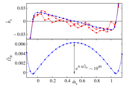
Figure 1: (color online) Top: Tethered field $\langle\hat{b}_{\text{s}}\rangle_{\hat{m},\hat{m}_{\text{s}}}$, Eq. (5), at $T=1.6$ and $\hat{m}=0.11$, for two individual samples of an $L=24$ system ($\square$ and $\blacksquare$) and for the sample average (•) as a function of $\hat{m}_{\text{s}}$. The field is self-averaging in the region outside the two external zeros. The errors cannot be seen at this scale. Bottom: Effective potential $\bar{\varOmega}_{N}(\hat{m}=0.11,\hat{m}_{\text{s}})$ obtained by integrating the averaged tethered field of the top panel. The two antiferromagnetic minima are separated by a very large barrier (the escape time is $\tau\sim\exp[N\Delta\bar{\varOmega}]$), and there is no paramagnetic minimum.

So far we have summarized the application of TMC for a single sample. Since it consists of simulations at fixed $(\hat{m},\hat{m}_{\text{s}})$, it eliminates the need to tunnel between coexisting phases and, hence, equilibrates the system much faster than a canonical simulation. However, we still face the serious problem of self-averaging violations. In principle, the definition of quenched disorder implies reconstructing the free energy with (4) before computing the disorder average. In this work, however, we sample average the Helmholtz potential rather than the free energy (a similar approach was taken in Ref. Fernandez et al., 2008).

In order to motivate this approach, let us consider Figure 1—Top. We compare the tethered average $\langle\hat{b}_{\text{s}}\rangle_{\hat{m},\hat{m}_{\text{s}}}$ for two individual samples with the disorder average over $1000$ samples. The zeros of this latter curve separate an internal gap with chaotic fluctuations, where the field vanishes in the thermodynamical limit, from an external region where the field is actually self-averaging.

We exploit the situation by considering a small, but finite, value of $h_{\text{s}}$. The saddle point defined by this field will be in the self-averaging region. We can therefore solve the saddle-point equations (7) on average, rather than sample by sample. Only afterwards do we make $h_{\text{s}}\to 0$ in the solution (this is analogous to the mathematical definition of spontaneous symmetry breaking). The limit $h_{\text{s}}=0^{+}$ is essentially equivalent to considering a ‘smeared’ saddle point and averaging over all $\hat{m}_{\text{s}}$

$$\overline{\langle O\rangle}_{\hat{m}}=\int\mathrm{d}\hat{m}_{\text{s}}\ \overline{\langle O\rangle}_{\hat{m},\hat{m}_{\text{s}}}\mathrm{e}^{-N[\bar{\varOmega}_{N}(\hat{m},\hat{m}_{\text{s}})-\varOmega_{0}]}\,.$$ (8)

$\varOmega_{0}$ is a normalization constant. Since we work at fixed $\hat{m}$, $\bar{\varOmega}_{N}$ is just the one-dimensional integral of $\overline{\langle\hat{b}_{\text{s}}\rangle}_{\hat{m},\hat{m}_{\text{s}}}$.

The other saddle-point equation, $\overline{\langle\hat{b}\rangle}_{\hat{m}}=\beta h$, defines a one-to-one relation $\hat{m}(h)$ so that $\overline{\langle O\rangle}_{\hat{m}(h)}$ and the canonical $\overline{\langle O\rangle}(h)$ both tend to the same thermodynamical limit (ensemble equivalence). Furthermore, for finite lattices $\overline{\langle O\rangle}_{\hat{m}}$ is better behaved statistically and arguably more faithful to the physics of an experimental sample. Therefore, we shall identify $\overline{\langle O\rangle}(h)=\overline{\langle O\rangle}_{\hat{m}(h)}$ and use the more familiar canonical notation. See Refs. Fernandez et al., 2009; Martin-Mayor et al., 2011 for a more detailed study of this ensemble equivalence.

We have used the above outlined procedure to thermalize the DAFF for temperatures down to $T=1.6$ and sizes up to $L=32$ ($1000$ samples for $L=8,12,16,24$ and $700$ samples for $L=32$). For each size we simulate a grid of $\approx 150$ points in the $(\hat{m},\hat{m}_{\text{s}})$ plane ($5$ values of $\hat{m}$, and $\approx 30$ values of $\hat{m}_{\text{s}}$ on each). We also use temperature parallel tempering. This is only necessary to thermalize $L\geq 24$, but it is convenient for smaller lattices because we are also interested in the $T$ dependence. Thermalization is ensured using the methods described in Ref. Álvarez Baños et al., 2010a. We provide more technical details in Ref. Martin-Mayor et al., 2011.

The first interesting physical result is the effective potential itself. Some authors have found metastable behavior in the DAFF, interpreted as a sign of a first-order transition. Sourlas (1999); *maiorano:07 This should manifest as the coexistence of antiferromagnetic and paramagnetic minima in $\bar{\varOmega}$. However, see Figure 1—Bottom, our results exhibit only two antiferromagnetic minima, separated by a very large free-energy barrier. In a canonical simulation, the system tunnels back and forth between the two, with an escape time $\tau\sim\exp[N\Delta\bar{\varOmega}]$. This explains the metastable behavior observed in previous work (and the difficulty to thermalize large samples with canonical methods), but is inconsistent with a first-order scenario.

Of course, we could be looking at a value of $\hat{m}$ (equivalently, of $h$) far from the critical point. In order to find the phase transition, we compute the usual second-moment correlation length $\xi$. Ballesteros et al. (1996) We use the propagator $F_{h}(\boldsymbol{k})=N\overline{\langle\phi(\boldsymbol{k})\phi(-\boldsymbol{k})\rangle}(h)$, where $\phi$ is the staggered Fourier transform of the spin field.

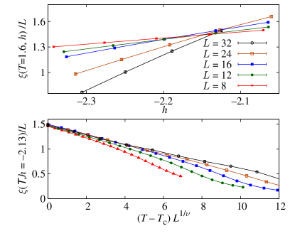
Figure 2: (color online) Top: Correlation length $\xi/L$ as a function of the applied magnetic field $h$ for $T=1.6$. The curves intersect, marking a second-order phase transition. Bottom: Scaling plot of $\xi$ as a function of $T$ for $h=-2.13$, showing large corrections to leading scaling (we use $\nu=1.05$).

We have plotted $\xi(h)/L$ at $T=1.6$ as a function of the applied field $h$ in Figure 2—Top. The curves for different $L$ show very clear intersections, marking the onset of a second-order phase transition. In order to estimate the critical exponents, we apply the quotients method. Ballesteros et al. (1996) We consider the ratios of physical observables for system sizes $(L,2L)$, computed at the intersection point $h^{*}(L)$ of their respective $\xi(h)/L$. We have applied this method to $\partial_{h}\xi\sim L^{1+1/\nu_{h}}$ and $\overline{\langle m_{\text{s}}^{2}\rangle}(h)\sim L^{2\beta/\nu_{h}-3}$ in Table 1. Note that our estimate for $\beta$ is very low, in accordance with previous numerical and experimental work.

We can also estimate $\nu$ from the temperature dependence of $\xi$ at fixed $h$, obtaining a second estimate $\nu_{T}$ (Table 1). Both determinations of $\nu$ should coincide, but we obtain $\nu_{h}\approx 0.75$ and $\nu_{T}\approx 1.05$. We can see in Figure 2—Bottom that this discrepancy is due to strong scaling corrections. If one attempts a collapse of the curves, focusing on different ranges for $\xi/L$, the corresponding values of $\nu$ vary from $\nu\approx 0.75$ to $\nu>2$, which explains the wide range of variation in previous numerical estimates of $\nu$. By safely locating the critical point and using the quotients method, we have minimized the scaling corrections, but not eliminated them completely.

$L$	$h^{*}(L)$	$\beta/\nu_{h}$	$\nu_{h}$	$\alpha/\nu_{h}$	$\nu_{T}$
8	$-2.178(4)$	0.0125(7)	0.887(5)	0.0765(25)	1.07(9)
12	$-2.140(5)$	0.0104(5)	0.790(9)	0.0781(27)	1.01(4)
16	$-2.123(3)$	0.0119(4)	0.742(7)	0.224(4)	1.10(15)

Table 1: Computation of the critical exponents using the quotients method. We extract our estimates from ratios of physical observables for sizes $(L,2L)$, computed at the intersection point of $\xi/L$. The first four columns give results for fixed $T=1.6$ and the last one at fixed $h=-2.13$.

We need an additional critical exponent in order fully to characterize the critical behavior of the DAFF. This is the hyperscaling violations exponent $\theta$, which can be related to the free-energy barrier between the ordered and the disordered phase: $\Delta F\propto L^{\theta}$. Vink et al. (2010); *fischer:11 The computation of these barriers is very difficult with traditional methods, but straightforward with TMC. Indeed, we can identify $\Delta F$ with the $\Delta\bar{\varOmega}_{N}$ between the two saddle points (disordered and antiferromagnetic) defined by the critical $h_{\text{c}}$.

$L$	$\Delta F/N$	Fit range	$\theta$	$\chi^{2}/\mathrm{d.o.f.}$
8	0.03382(29)	$L\geq 8\$	$1.448(9)$	5.56/3
12	0.01756(15)	$L\geq 12$	$1.469(13)$	0.44/2
16	0.01138(9)	$L\geq 16$	$1.461(20)$	0.16/1
24	0.00608(5)
32	0.00392(5)

Table 2: Computation of the hyperscaling violations exponent $\theta$ from the free-energy barriers $\Delta F$. We report fits to $\Delta F=AL^{\theta}$, for different ranges, giving the $\chi^{2}$ and the degrees of freedom of each fit. Our preferred final estimate is $\theta=1.469(20)$, taking the central value of the fit for $L\geq 12$ and the more conservative error of the fit for $L\geq 16$.

We can compute this barrier simply by evaluating the line integral of $\bigl{(}\overline{\langle\hat{b}\rangle}_{\hat{m},\hat{m}_{\text{s}}}-\beta h_{\text{c}},\ \overline{\langle\hat{b}_{\text{s}}\rangle}_{\hat{m},\hat{m}_{\text{s}}}\bigr{)}$ along a path joining the two saddle points. We know that one of them will lie on the line $\hat{m}_{\text{s}}=0.5$ ($m_{\text{s}}\approx 0$). Therefore, we first integrate from the antiferromagnetic saddle point to $\hat{m}_{\text{s}}=0.5$ at fixed $\hat{m}$. We then integrate at fixed $\hat{m}_{\text{s}}=0.5$ until we reach the disordered saddle point. We give the resulting values of $\Delta\bar{\varOmega}_{N}=\Delta F/N$ in Table 2. Our final estimate is $\theta=1.469(20)$, incompatible with the $\theta=D-1$ of a first-order phase transition.

Notice that the hyperscaling relation $2-\alpha=\nu(D-\theta)$, coupled with our values for $\nu$ and $\theta$, predicts not only a divergence of the specific heat, as observed in experiments, but also a positive $\alpha$. We could test this result directly by computing $C=\partial_{h}\overline{\langle m\rangle}$. Unfortunately, the quotients method is ill-suited to this quantity, whose scaling is more aptly described as $C\simeq A+BL^{\alpha/\nu}$. Ballesteros et al. (1998) Therefore, one needs extremely large values of $L$ to reach the asymptotic regime $C\sim L^{\alpha/\nu}$. The behavior of the quotients in Table 1 is consistent with this expectation.

It has been proposed that $\theta$ is not independent, but given by $\theta=D/2-\beta/\nu$. Schwartz and Soffer (1985); *schwartz:86 Combining Tables 1 and 2 we see that our numerical results are indeed compatible with this two-exponent scenario.

We can use our results to comment on the experimental situation. In an experimental study, the critical exponents are computed from fits to the scattering line shape $S(k)=S_{\text{d}}(k)+S_{\text{c}}(k)$, where the two terms distinguish connected and disconnected contributions. In the two-exponent scenario, strongly supported by our data, the most singular term in $S_{\text{d}}$ is the square of $S_{\text{c}}$. This Ansatz was applied in Ref. Slanic et al., 1999, yielding $\nu=0.87(7)$ and $\eta=0.16(6)$. Since $\eta=\theta-1+2\beta/\nu$, however, this last value violates hyperscaling bounds and is also incompatible with our results. Perhaps taking $S_{\text{d}}=(S_{\text{c}})^{2}$ for the whole function, not just its singularity, is an excessive simplification. Clearly a better theoretical determination of $S(k)$ is needed. Our methods are well suited to a direct numerical approach to this question.

We have used the tethered formalism to obtain a comprehensive picture of the critical behavior of the DAFF, resolving the inconsistencies in previous work. This method restores self-averaging to the problem and is capable of handling rugged free-energy landscapes to equilibrate much larger systems than canonical parallel tempering. Our simulations show clear signs of a second-order phase transition and are consistent both with experiments on the DAFF and with analytical results for the RFIM. The critical exponents $\theta$ and $\beta/\nu$ (equivalently, $\eta$ and $\bar{\eta}$) are computed with a high precision, although our simulations were not optimized for the computation of $\nu$ (equivalently, of $\alpha$). We obtain $\nu=0.90(15)$, consistent with a positive $\alpha$.

The tethered approach demonstrated in this paper has a very broad scope and we believe it can be fruitfully applied to many systems featuring large free-energy barriers. Indeed, it has already been successfully implemented for hard-spheres crystallization. Fernández et al. (2011) Other promising avenues are the study of Goldstone bosons and the equation of state for the $D=3$ spin glass, Álvarez Baños et al. (2010b) or equilibrium and aging relaxation in a metastable phase (e.g., to prevent crystallization of supercooled liquids, see Ref. Fernandez et al., 2006).

We thank N.G. Fytas for his comments on our manuscript. Our simulations were performed on the Red Española de Supercomputación and at BIFI (Terminus and Piregrid). We acknowledge partial financial support from MICINN, Spain, (contract no FIS2009-12648-C03) and from UCM-Banco de Santander (GR32/10-A/910383). DY was supported by the FPU program (Spain).

References

- Nattermann (1998) T. Nattermann, in Spin glasses and random fields, edited by A. P. Young (World Scientific, Singapore, 1998).
- Belanger (1997) D. P. Belanger, ibid .
- Slanic et al. (1999) Z. Slanic, D. P. Belanger, and J. A. Fernandez-Baca, Phys. Rev. Lett. 82, 426 (1999).
- Ye et al. (2004) F. Ye, et al., J. Magn. & Magn. Mater. 272, 1298 (2004).
- Belanger et al. (1983) D. P. Belanger, A. R. King, V. Jaccarino, and J. L. Cardy, Phys. Rev. B 28, 2522 (1983).
- Belanger and Slanic (1998) D. P. Belanger and Z. Slanic, J. Magn. and Magn. Mat. 186, 65 (1998).
- Middleton and Fisher (2002) A. A. Middleton and D. S. Fisher, Phys. Rev. B 65, 134411 (2002).
- Hartmann and Young (2001) A. K. Hartmann and A. P. Young, Phys. Rev. B 64, 214419 (2001).
- Malakis and Fytas (2006) A. Malakis and N. G. Fytas, Phys. Rev. E 73, 016109 (2006).
- Sourlas (1999) N. Sourlas, Comp. Phys. Comm. 121, 183 (1999).
- Wu and Machta (2006) Y. Wu and J. Machta, Phys. Rev. B 74, 064418 (2006).
- Maiorano et al. (2007) A. Maiorano, V. Martin-Mayor, J. J. Ruiz-Lorenzo, and A. Tarancón, Phys. Rev. B 76, 064435 (2007).
- Parisi and Sourlas (2002) G. Parisi and N. Sourlas, Phys. Rev. Lett. 89, 257204 (2002).
- Fytas and Malakis (2011) N. G. Fytas and A. Malakis, Eur. Phys. J. B 79, 13 (2011).
- Fernandez et al. (2009) L. A. Fernandez, V. Martin-Mayor, and D. Yllanes, Nucl. Phys. B 807, 424 (2009).
- Martin-Mayor et al. (2011) V. Martin-Mayor, B. Seoane, and D. Yllanes, J. Stat. Phys. 144, 554 (2011).
- Fernandez et al. (2008) L. A. Fernandez, A. Gordillo-Guerrero, V. Martin-Mayor, and J. J. Ruiz-Lorenzo, Phys. Rev. Lett. 100, 057201 (2008).
- Álvarez Baños et al. (2010a) R. A. Baños, et al., J. Stat. Mech. , P06026 (2010a).
- Ballesteros et al. (1996) H. G. Ballesteros, L. A. Fernandez, V. Martin-Mayor, and A. Muñoz Sudupe, Phys. Lett. B 378, 207 (1996).
- Vink et al. (2010) R. L. C. Vink, T. Fischer, and K. Binder, Phys. Rev. E 82, 051134 (2010).
- Fischer and Vink (2011) T. Fischer and R. L. C. Vink, J. Phys. Condens. Matt. 23, 234117 (2011).
- Ballesteros et al. (1998) H. G. Ballesteros, et al., Phys. Rev. B 58, 2740 (1998).
- Schwartz and Soffer (1985) M. Schwartz and A. Soffer, Phys. Rev. Lett. 55, 2499 (1985).
- Schwartz and Soffer (1986) M. Schwartz and A. Soffer, Phys. Rev. B 33, 2059 (1986).
- Fernández et al. (2011) L. Fernández, V. Martin-Mayor, B. Seoane, and P. Verrocchio, (2011), arXiv:1103.2599 .
- Álvarez Baños et al. (2010b) R. A. Baños, et al., Phys. Rev. Lett. 105, 177202 (2010b).
- Fernandez et al. (2006) L. A. Fernandez, V. Martin-Mayor, and P. Verrocchio, Phys. Rev. E 73, 020501 (2006).