Numerical solution of $Q^{2}$ evolution equations
for fragmentation functions

Abstract

Semi-inclusive hadron-production processes are becoming important in high-energy hadron reactions. They are used for investigating properties of quark-hadron matters in heavy-ion collisions, for finding the origin of nucleon spin in polarized lepton-nucleon and nucleon-nucleon reactions, and possibly for finding exotic hadrons. In describing the hadron-production cross sections in high-energy reactions, fragmentation functions are essential quantities. A fragmentation function indicates the probability of producing a hadron from a parton in the leading order of the running coupling constant $\alpha_{s}$. Its $Q^{2}$ dependence is described by the standard DGLAP (Dokshitzer-Gribov-Lipatov-Altarelli-Parisi) evolution equations, which are often used in theoretical and experimental analyses of the fragmentation functions and in calculating semi-inclusive cross sections. The DGLAP equations are complicated integro-differential equations, which cannot be solved in an analytical method. In this work, a simple method is employed for solving the evolution equations by using Gauss-Legendre quadrature for evaluating integrals, and a useful code is provided for calculating the $Q^{2}$ evolution of the fragmentation functions in the leading order (LO) and next-to-leading order (NLO) of $\alpha_{s}$. The renormalization scheme is $\overline{MS}$ in the NLO evolution. Our evolution code is explained for using it in one’s studies on the fragmentation functions.

PROGRAM SUMMARY

Program Title: ffevol1.0
Journal Reference:
Catalogue identifier:
Licensing provisions: none
Programming language: Fortran77
Computer: HP DL360G5-DC-X5160
Operating system: Linux 2.6.9-42.ELsmp
RAM: 130 M bytes
Keywords: Fragmentation function, $Q^{2}$ evolution, Quark, Gluon, QCD
Classification: 11.5 Quantum Chromodynamics, Lattice Gauge Theory
Nature of problem:
This program solves timelike DGLAP $Q^{2}$ evolution equations with or without next-to-leading-order $\alpha_{s}$ effects for fragmentation functions. The evolved functions can be calculated for $D_{g}^{h}$, $D_{u}^{h}$, $D_{\bar{u}}^{h}$, $D_{d}^{h}$, $D_{\bar{d}}^{h}$, $D_{s}^{h}$, $D_{\bar{s}}^{h}$, $D_{c}^{h}$, $D_{\bar{c}}^{h}$, $D_{b}^{h}$, and $D_{\bar{b}}^{h}$ of a hadron $h$.
Solution method:
The DGLAP integrodifferential equations are solved by the Euler’s method for the differentiation of $\ln Q^{2}$ and the Gauss-Legendre method for the $x$ integral as explained in section 4.
Restrictions:
This program is used for calculating Q² evolution of fragmentation functions in the leading order or in the next-to-leading order of $\alpha_{s}$. $Q^{2}$ evolution equations are the timelike DGLAP equations. The double precision arithmetic is used. The renormalization scheme is the modified minimal subtraction scheme ($\overline{MS}$). A user provides initial fragmentation functions as the subroutines FF_INI and HQFF in the end of the distributed code FF_DGLAP.f. In FF_DGLAP.f, the subroutines are give by taking the HKNS07 hkns07 functions as an example of the initial functions. Then, the user inputs kinematical parameters in the file setup.ini as explained in section 5.2.
Running time:
A few seconds on HP DL360G5-DC-X5160.

1 Introduction

In the recent years, semi-inclusive hadron-production processes are becoming more and more important for studying internal structure of hadrons and heavy-ion reactions. There are three ingredients for calculating their cross sections in high-energy reactions with large transverse momenta for produced hadrons. The first part is on parton distribution functions (PDFs) of initial hadrons, the second is on partonic cross sections, and the third is on fragmentation functions (FFs) for describing production of hadrons ffs_before_2006 ; hkns07 ; hkos08 ; ffs-recent ; ffs-summary . The perturbative aspect of quantum chromodynamics (QCD) has been established for many processes, so that the elementary partonic cross sections of the second part can be accurately calculated in high-energy processes. The PDFs of the first part have been extensively investigated mainly by inclusive deep inelastic scattering. Except for extreme kinematical conditions, the unpolarized PDFs are generally well determined. For example, one may look at Ref. recent-unpol-pdfs for the situation of unpolarized PDFs, Refs. aac ; other-pol-pdfs for polarized PDFs, and Refs. our-npdfs ; other-recent-npdfs for nuclear PDFs. Because the PDF and partonic cross section parts are relatively well known, the only issue is the accuracy of the FFs of the third part for calculating precise semi-inclusive cross sections.

The first estimate for uncertainties of the FFs was done in Ref. hkns07 , and its results indicated that they have large uncertainties especially for so called disfavored fragmentation functions. This fact could add ambiguities to calculated cross sections of high-energy hadron productions such as $\vec{p}+\vec{p}\rightarrow\pi+X$ and $A+A^{\prime}\rightarrow h+X$ at RHIC and LHC. Here, where $\vec{p}$ and $\pi$ indicate a polarized proton and a pion, respectively, $X$ indicates a sum over all other hadrons created in the reaction, $A$ and $A^{\prime}$ are nuclei, and $h$ is a produced hadron. Furthermore, the FFs could be also used for other studies in searching for exotic hadrons by noting characteristic differences in favored and disfavored FFs as pointed out in Ref. hkos08 .

These topics suggest that the FFs should be one of most important quantities in describing high-energy hadron reactions. There are two important variables in the FFs. One is the energy fraction $x$ (or often denoted as $z$) for a produced hadron from a parton and the other is the hard scale $Q^{2}$. Definitions of these quantities are given in Sec. 2. The $x$-dependent functions are determined mainly from experimental measurements of electron-positron annihilation processes $e^{+}+e^{-}\rightarrow h+X$ by a global analysis ffs_before_2006 ; hkns07 ; hkos08 ; ffs-recent . On the other hand, $Q^{2}$ dependence can be calculated in perturbative QCD. The standard equations for describing $Q^{2}$ variations are the timelike DGLAP evolution equations dglap .

The evolution equations are complicated integro-differential equations, which cannot be solved by an analytical method, especially if higher-order corrections are included in the equations. They are solved by numerical methods. A popular method is to use the Mellin transformation mellin , in which $Q^{2}$ evolution of moments for the FFs is analytically calculated and resulting moments are then transformed into $x$-dependent functions by the inverse Mellin transformation. One of other numerical methods is to solve the $x$-integral part by dividing the $x$ axis into small steps for calculating integrals bfevol ; trans-evol , which is so called brute-force or Euler method. Of course, the integral could be calculated by a better method such as the Simpson method or Gauss-Legendre quadrature. Another approach is to expand the FFs and DGLAP splitting functions in terms of orthogonal polynomials such as the Laguerre polynomials lag . Advantages and disadvantages of these numerical methods are explained in Ref.kn04 . There are also recent studies on the numerical solution recent .

Although the FFs are important, it is unfortunate that no useful code is available in public for calculating $Q^{2}$ variations of the FFs. For example, the FFs are calculated in a theoretical model bentz at a typical hadron scale of small $Q^{2}$. In order to compare with the FFs obtained by global analyses or with experimental data, one needs to calculate the $Q^{2}$ evolution. However, one should make one’s own code or rely on a private communication for obtaining a code since no public code is available, although the $Q^{2}$ evolution is often used also in theoretical and experimental analyses. In this work, we explain our method for solving the DGLAP evolution and a useful code is supplied for public use.

This paper consists of the following. The fragmentation functions and their kinematical variables are introduced in Sec. 2, and evolution equations are explained in Sec. 3. Our numerical method is described in Sec. 4 for solving the DGLAP $Q^{2}$ evolution equations, and a developed evolution code is explained in Sec. 5. Numerical results are shown in Sec. 6 by running the evolution code, and our studies are summarized in Sec. 7.

2 Fragmentation functions

Fragmentation functions are given in the electron-positron annihilation process $e^{+}+e^{-}\rightarrow h+X$, where $h$ indicates a specific hadron. The process is described first by a $q\bar{q}$ creation by $e^{+}e^{-}\rightarrow q\bar{q}$ and a subsequent fragmentation, namely a hadron-$h$ creation from the primary quark or antiquark. The fragmentation function is defined by the hadron-production cross section of $e^{+}+e^{-}\rightarrow h+X$ as esw-book :

$$F^{h}(x,Q^{2})=\frac{1}{\sigma_{tot}}\frac{d\sigma(e^{+}e^{-}\rightarrow hX)}{dx},$$ (1)

where $\sigma_{tot}$ is the total hadronic cross section. The variable $Q^{2}$ is the virtual photon or $Z^{\,0}$ momentum squared in $e^{+}e^{-}\rightarrow\gamma$ (or $Z^{\,0}$) and it is expressed by the center-of-mass energy $\sqrt{s}$ as $Q^{2}=s$. The variable $x$ is the hadron energy $E_{h}$ scaled to the beam energy $\sqrt{s}/2$, and it is defined by the fraction:

$$x\equiv\frac{E_{h}}{\sqrt{s}/2}=\frac{2E_{h}}{\sqrt{Q^{2}}}.$$ (2)

The fragmentation process is described by the summation of hadron productions from primary quarks, antiquarks, and gluons esw-book :

$$F^{h}(x,Q^{2})=\sum_{i}C_{i}(x,\alpha_{s})\otimes D_{i}^{h}(x,Q^{2}),$$ (3)

where $C_{i}(x,\alpha_{s})$ is a coefficient function, and it is calculated in perturbative QCD qqbar-cross . The factor $\alpha_{s}(Q^{2})$ is the running coupling constant, and its expression is given in Appendix A for the leading order (LO) and next-to-leading order (NLO). The function $D_{i}^{h}(x,Q^{2})$ is the fragmentation function from a parton $i$ ($=u,\ d,\ s,\ \cdot\cdot\cdot,\ g$) to a hadron $h$, and it is the probability of producing the hadron $h$, in the LO of $\alpha_{s}$, from the parton $i$ with the energy fraction $x$ and the momentum square scale $Q^{2}$. The notation $\otimes$ indicates a convolution integral defined by

$$f(x)\otimes g(x)=\int^{1}_{x}\frac{dy}{y}f(y)g\left(\frac{x}{y}\right).$$ (4)

The fragmentation function is formally given by the expression ffs-def

$$D_{i}^{h}(x)=\sum\limits_{X}\int\frac{dy^{-}}{24\pi}e^{ik^{+}y^{-}}{\rm{Tr}}\left[{\gamma^{+}\left\langle{0\left|{\left.{\left.\psi_{i}(0,y^{-},0_{\bot})\right|h,X}\right\rangle\left\langle{h,X\left|{\bar{\psi}_{i}(0)}\right.}\right.}\right|0}\right\rangle}\right],$$ (5)

where $k$ is the parent quark momentum, the lightcone notation is defined by $a^{\pm}=(a^{0}\pm a^{3})/\sqrt{2}$, the variable $x$ is then given by $x=p_{h}^{+}/k^{+}$ with the hadron momentum $p_{h}$, and $\perp$ is the direction perpendicular to the third coordinate. A gauge link needs to be introduced in Eq. (5) so as to satisfy the color gauge invariance. It should be, however, noted that a lattice QCD calculation is not available for the FFs because the operator-product-expansion method cannot be applied due to the fact that a specific hadron $h$ should be observed in the final state with the momentum $p_{h}$.

An important sum rule of the FFs is on the energy conservation. Since the variable $x$ is the energy fraction for the produced hadron, its sum weighted by the fragmentation functions, namely the sum of their second moments, should be one.

$$\sum_{h}M_{i}^{h}=\sum_{h}\int_{0}^{1}dx\,x\,D_{i}^{h}(x,Q^{2})=1.$$ (6)

The fragmentation function should vanish kinematically at $x=1$ and it is expected to be a smooth function at small $x$, so that it is typically parametrized in the form ffs_before_2006 ; hkns07 ; hkos08 ; ffs-recent

$$D_{i}^{h}(x,Q_{0}^{2})=N_{i}^{h}x^{\alpha_{i}^{h}}(1-x)^{\beta_{i}^{h}},$$ (7)

at fixed $Q^{2}$ ($\equiv Q_{0}^{2}$). Current experimental data are not accurate enough to find much complicated $x$-dependent functional form. In order to calculate the function $D_{i}^{h}(x,Q^{2})$ at arbitrary $Q^{2}$, one should rely on $Q^{2}$ evolution equations and the standard ones are the DGLAP equations in the next section.

3 $Q^{2}$ evolution equations

The FFs depend on two variables $x$ and $Q^{2}$. The $x$-dependence is associated with a non-perturbative aspect of QCD, so that the only way of calculating it theoretically is to use hadron models, because the lattice QCD estimate is not available for the FFs. There are some hadron-model calculations bentz by using the expression Eq. (5) at a small hadronic $Q^{2}$ scale. On the other hand, $x$-dependent functions are determined by global analyses of experimental data mainly on $e^{+}+e^{-}\rightarrow h+X$ ffs_before_2006 ; hkns07 ; hkos08 ; ffs-recent . In the model calculations and also in the global analyses, the $Q^{2}$ dependence or so called scaling violation is calculated in perturbative QCD.

The $Q^{2}$ dependence of the FFs is described by the DGLAP evolution equations in the same way with the ones for the PDFs with slight modifications in splitting functions. They are generally given by dglap ; esw-book

$$\frac{\partial}{\partial\ln Q^{2}}D_{q^{+}_{i}}^{h}(x,Q^{2}) =\frac{\alpha_{s}(Q^{2})}{2\pi}\,\left[\sum_{j}P_{q_{j}q_{i}}(x,\alpha_{s})\otimes D_{q^{+}_{j}}^{h}(x,Q^{2})+2P_{gq}(x,\alpha_{s})\otimes D_{g}^{h}(x,Q^{2})\right],$$

$$\frac{\partial}{\partial\ln Q^{2}}D_{g}^{h}(x,Q^{2}) =\frac{\alpha_{s}(Q^{2})}{2\pi}\,\left[P_{qg}(x,\alpha_{s})\otimes\sum_{j}D_{q^{+}_{j}}^{h}(x,Q^{2})+P_{gg}(x,\alpha_{s})\otimes D_{g}^{h}(x,Q^{2})\right],$$ (8)

where $D_{q^{+}}^{h}(x,Q^{2})$ denotes the fragmentation-function combination $D_{q}^{h}(x,Q^{2})+D_{\bar{q}}^{h}(x,Q^{2})$. If the sum is taken over the flavor, it becomes the singlet function $D_{q_{s}}^{h}(x,Q^{2})=\sum_{q}[D_{q}^{h}(x,Q^{2})+D_{\bar{q}}^{h}(x,Q^{2})]$, and $N_{f}$ is the number of quark flavors. The flavor nonsinglet evolution, for example, for $q-\bar{q}$ type function is described by

$$\frac{\partial}{\partial\ln Q^{2}}D_{q_{i}^{-}}^{h}(x,Q^{2})=\frac{\alpha_{s}(Q^{2})}{2\pi}\,\sum_{j}P_{q_{j}q_{i}}(x,\alpha_{s})\otimes D_{q_{j}^{-}}^{h}(x,Q^{2}),$$ (9)

where $D_{q^{-}_{i}}^{h}(x,Q^{2})=D_{q_{i}}^{h}(x,Q^{2})-D_{\bar{q}_{i}}^{h}(x,Q^{2})$. The functions $P_{qq}(x)$, $P_{gq}(x)$, $P_{qg}(x)$, and $P_{gg}(x)$ are time-like splitting functions, and $P_{ij}(x)$ describes the splitting probability that the parton $j$ splits into $i$ with the momentum fraction $x$. It should be noted that $P_{gq}(x)$ and $P_{qg}(x)$ are interchanged in the splitting function matrix for the PDFs. The LO splitting functions are the same as the space-like ones; however, there are differences between them in the NLO and higher orders esw-book ; splitting . Actual expressions of the LO splitting functions are provided in Appendix B. The NLO expressions should be found in Ref. esw-book because they are rather lengthy.

The DGLAP equations in Eq. (8) are coupled integro-differential equations with complicated $x$-dependent functions especially if higher-order $\alpha_{s}$ corrections are taken into account. It is obvious that they cannot be solved in a simple analytical form. The convolution integral is generally expressed by a simple multiplication of Mellin moments, so that the the equations are easily solved in the Mellin-moment space. However, the inverse Mellin transformation should be calculated by a numerical method in any case to obtain the $x$-dependent function. Here, we solve the DGLAP equations directly in the $x$ space by calculating the $x$ integral in a numerical way. Advantages and disadvantages of both methods are discussed in Ref. kn04 .

4 Numerical method for solving $Q^{2}$ evolution equations

The integro-differential equations of Eqs. (8) and (9) are solved in the following way. Scaling violation ($Q^{2}$ dependence) of the FFs is roughly given by $\ln Q^{2}$, which is defined as the variable $t$:

$$t=\ln Q^{2}.$$ (10)

Because the $t$ dependence is not complicated in the FFs, we do not have to use a sophisticated method for solving the differentiation. The following simple method is used for solving the differentiation:

$$\frac{df(t)}{dt}=\,\frac{f(t_{\ell+1})-f(t_{\ell})}{\Delta t}.$$ (11)

Here, the variable $t$ is divided into $N_{t}$ steps with a small interval $\Delta t$. This method could be called Euler method SIMP . It is also possible to use the Euler method for the integration part by dividing the $x$ region into $N_{x}$ steps with the interval $\Delta x$ bfevol . However, it is more desirable to use a better method since the $x$ dependencies of the FFs and splitting functions are not simple. Here, the Gauss-Legendre method is used for calculating the integral over $x$:

$$\int_{x_{0}}^{1}g(x)\ dx\simeq\frac{1-x_{0}}{2}\sum_{k=1}^{N_{GL}}\,w_{k}g(x_{k}),$$ (12)

where $x_{k}=[1+x_{0}+(1-x_{0})x_{k}^{\prime}]/2$ with the zero points $x_{k}^{\prime}$ of the Gauss-Legendre polynomials in the region $-1\leq x_{k}^{\prime}\leq+1$, $w_{k}$ are the weights recipes , and $N_{GL}$ is the number of Gauss-Legendre points. In our previous works bfevol ; trans-evol , simpler methods are used for calculating the integral by the Euler method and the Simpson’s one. Here, we change the method for the Gauss-Legendre one for getting more accurate numerical results.

In the following, only the nonsinglet evolution in Eq. (9) is discussed because an extension to the general evolution in Eq. (8) is obvious just by writing down two coupled equations in the same way. Substituting Eqs. (11) and (12) into the nonsinglet equation of Eq. (9), we obtain

$$D_{q_{i}^{-}}^{h}(x_{m},t_{\ell+1})=D_{q_{i}^{-}}^{h}(x_{m},t_{\ell})+\Delta t\,\frac{\alpha_{s}(t_{\ell})}{2\pi}\frac{1-x_{m}}{2}\sum_{j}\sum_{k=1}^{N_{GL}}w_{k}\,\frac{1}{x_{k}}\,P_{q_{j}q_{i}}(x_{k})\,D_{q_{j}^{-}}^{h}\left(\frac{x_{m}}{x_{k}},t_{\ell}\right).$$ (13)

In previous codes of $Q^{2}$ evolution equations in Refs. bfevol ; trans-evol , an option is provided to divide $\ln x_{Bj}$, where $x_{Bj}$ is the Bjorken scaling variable, into equal steps instead of linear-$x_{Bj}$ steps because the small-$x_{Bj}$ region is often important in discussing deep inelastic structure functions. However, the small-$x$ part is not as reliable as the PDF case because experimental data do not exist at very small $x$ and because of theoretical issues on finite hadron masses and resummation effects. The Gauss-Legendre points are taken by considering the linear-$x$ scale at $x>0.1$ and by the logarithmic-$x$ scale at $x<0.1$. If the initial function is supplied at certain $Q^{2}$ ($\equiv Q_{0}^{2}$), the evolution from $t_{1}=lnQ_{0}^{2}$ to the next point $t_{2}=t_{1}+\Delta t$ is calculated by Eq. (13). Repeating this step, we finally obtain the evolved FF at $t_{N+1}=\ln Q^{2}$.

The most important and time-consuming part is to calculate the $x$ integrals by the Gauss-Legendre quadrature. For the integral from the minimum $x_{0}$ to 1, the splitting functions $P_{q^{-}}(x_{k})$ are first calculated at $N_{GL}$ points of $x_{k}$ and they are stored in an array. Then, the fragmentation functions are also calculated at $x_{k}$ and $x_{m}$, and they are stored in a two-dimensional array. These arrays are used for calculating the Gauss-Legendre sum in Eq. (13).

5 How to run the $Q^{2}$ evolution code

We made the numerical evolution code of the FFs by the method discussed in the previous section. Its main code (FF_DGLAP.f), a test program (sample.f), and an example of the input file (setup.ini) could be obtained upon email request request . There are three major steps for calculating the $Q^{2}$ evolution of the FFs:

• Initial FFs are supplied in the subroutines, FF_INI for gluon ($g$) and light-quark ($u$, $d$, $s$, $\bar{u}$, $\bar{d}$, $\bar{s}$) functions and HQFF for heavy-quark ($c$, $b$) functions.

• Input parameters for the evolution are supplied in the file setup.ini. These parameters are used for calculating two-dimensional ($x$ and $Q^{2}$) grid data for the FFs in the ranges $x_{min}\leq x\leq 1$ and $Q_{0}^{2}=Q^{2}_{min}\leq Q^{2}\leq Q_{max}^{2}$.

• As indicated in the test code (sample.f), the evolved $Q^{2}$ value (Q2) and the value of $x$ (X) should be supplied for calculating the evolution. The grid data created in the step 2 are used for this final step calculation. Therefore, output functions can be obtained at various $x$ and $Q^{2}$ points without repeating the $Q^{2}$ evolution calculations as far as they are within the ranges $x_{min}\leq x\leq 1$ and $Q_{0}^{2}\leq Q^{2}\leq Q_{max}^{2}$.

5.1 Main evolution code

The main $Q^{2}$ evolution code (FF_DGLAP.f) is rather long, so that only the major points are explained. First, one needs to supply the initial FFs in the subroutines FF_INI and HQFF, which are located in the end of FF_DGLAP.f. The subroutine FF_INI is for gluon ($g$) and light-quark ($u$, $d$, $s$, $\bar{u}$, $\bar{d}$, $\bar{s}$) functions, and HQFF is for heavy-quark ($c$, $b$) functions. As an example, the HKNS07 functions hkns07 are given. The initial scale for the gluon and light-quark functions is $Q_{0}^{2}$, and the scales are the mass-threshold values $m_{c}^{2}$ and $m_{b}^{2}$ for charm and bottom FFs, respectively. These scale values are provided in setup.ini, and the initial functions are supplied in analytical forms in our main code FF_DGLAP.f.

Second, input parameters are read from setup.ini, which is explained in Sec. 5.2. They are basic parameters: the order of $\alpha_{s}$, scale parameter of QCD ($\Lambda$), charm and bottom masses $m_{c}$ and $m_{b}$ for setting thresholds, number of flavors at the initial scale $Q_{0}^{2}$; kinematical parameters: initial scale $Q_{0}^{2}$, maximum $Q^{2}$ value $Q^{2}_{max}$, and minimum $x$ ($x_{min}$) for making grid data of the evolved FFs; parameters to control the numerical integrations: Gauss-Legendre points ($N_{GL}$) and numbers of $\ln Q^{2}=t$ and $x$ points ($N_{t}$ and $N_{x}$).

Third, the splitting functions are calculated at the points $x_{k}$ for calculating the summation in Eq. (13). The $x_{k}$ points are determined by the parameters $N_{x}$ and $N_{GL}$. The splitting functions at these points are calculated at once in the beginning of this code. In the same way, the initial FFs are also calculated at the given points of $x_{k}$ and $x_{m}$ and they are stored in two-dimensional ($k$ and $m$) arrays.

Forth, the evolution step of Eq. (13) is repeated in $N_{t}$ times to obtain the evolved FFs up to $Q_{max}^{2}$ from $Q_{0}^{2}$ in the range $x_{min}\leq x\leq 1$. If $Q^{2}$ exceeds the threshold $m_{c}^{2}$ (or $m_{b}^{2}$), the number of flavor is changed accordingly and charm (or bottom) function starts to participate in the evolution calculation. During the evolution calculations, two dimensional ($x$ and $Q^{2}$) grid data are stored for calculating the FFs at any point within the ranges $x_{min}<x<1$ and $Q_{0}^{2}<Q^{2}<Q_{max}^{2}$ by interpolation. The $x$ and $Q^{2}$ values need to be specified in running this main subroutine, and an example is proved as a test code (sample.f).

5.2 Input file

The input parameters should be supplied in the file setup.ini for running the main evolution routine FF_DGLAP.f, in which the parameter values are read. For example, the following input values are used for evolving the HKNS07 FFs in the NLO. Here, the symbol # is for commenting out the subsequent line in setup.ini.

# pQCD ORDER 1:LO, 2:NLO

IORDER= 2

# DLAM (Scale parameter in QCD) of $$N_{f}=4$$

# e.g. 0.220 GeV (LO), 0.323 GeV (NLO) in HKNS07

DLAM= 0.323 # in HKNS07-NLO

# Heavy-quark mass threshold

# HQTHRE= $$m_{c} m_{b}$$, = 1.43, 4.3 GeV in HKNS07

HQTHRE= 1.43, 4.3

# Q2 range for making grid files

# Q02 $$\rightarrow$$ Q2max (note: not the Q2 evolution range)

Q2= 1.D0, 1558.D+5 # in HKNS07 Library

# minimum of $$x$$

XMIN= 1.D-2

# NT: # of t-steps for $$Q^{2}$$ dependence

# NX: # of x-steps for $$xD(x)$$

# NGLI: # of steps for Gauss-Legendre integral

NT= 580

NX= 160

NGLI= 32

# NF at the initial scale Q02

NF= 3 (14)

The parameter IORDER indicates the LO or NLO of $\alpha_{s}$. Both LO and NLO evolutions are possible so that the order of $\alpha_{s}$ should be IORDER=1 or 2. The scale parameter $\Lambda$ should be supplied in the case of four flavors ($\Lambda_{4}$). It is then converted to the three and five flavor values ($\Lambda_{3}$ and $\Lambda_{5}$) within the evolution code roberts-book . The charm and bottom functions appear as finite distributions above the threshold values $Q^{2}>m_{c}^{2}$ (or $m_{b}^{2}$). The HQTHRE values are these heavy-quark thresholds threshold .

The kinematical regions of $x$ and $Q^{2}$ are specified by the parameters, $Q_{0}^{2}$ (=$Q_{min}^{2}$), $Q_{max}^{2}$, and $x_{min}$. The $Q_{0}^{2}$ is the initial $Q^{2}$ scale, and $Q_{max}^{2}$ is the maximum $Q^{2}$ for calculating the FFs. Any $Q^{2}$ values can be chosen as long as perturbative QCD calculations are valid, which means that small $Q_{0}^{2}$ and $Q_{max}^{2}$ values are not favorable particularly in the region $Q^{2}<1$ GeV² where pQCD calculations do not converge easily due to the large running coupling constant $\alpha_{s}$. The $Q^{2}$ maximum $Q^{2}_{max}=1.558\times 10^{8}$ GeV² is used in making the HKNS07 library for their FFs hkns07 . It is chosen so that two grid points are close to the charm and bottom threshold values $m_{c}^{2}$ and $m_{b}^{2}$. If one needs to calculate the evolution only to $Q^{2}$=100 GeV², one does not have to take such a large $Q^{2}_{max}$, and $Q^{2}_{max}$=100 GeV² is enough. We also should note that a very small value of $x_{min}$ is not favored because some FFs become negative, which is not physically allowed in principle. This occurs due to a singular behavior of a time-like splitting function. In order to cure this issue, more detailed studies are needed by including resummation effects resum .

The parameter NT is the number of points of $\ln Q^{2}$ in the range $\ln Q^{2}_{min}\leq\ln Q^{2}\leq\ln Q^{2}_{max}$, and NX is the number of points of $x$ in the range $x_{min}\leq x\leq 1$. The NGLI is the Gauss-Legendre points for numerical integration. In the example of Eq. (14), the number of $t=\ln Q^{2}$ points is 580, the one of $x$ is 160, and the one of the Gauss-Legendre points is 32. They are selected by looking at evolution results by varying their values. Such studies are explained in details in Sec. 6. The NF is the number of flavors at $Q_{0}^{2}$, and it is usually three as given in Eq. (14).

5.3 Sample code

A test code (sample.f) is provided as an example for running the main evolution code. The main evolution routine GETFF(Q2,X,FF) is called by supplying $Q^{2}$ and $x$ values. Evolved FFs are returned to FF(I), (I=$-$5, 5):

$$FF(-5)=D_{\bar{b}}^{h}(x,Q^{2}), FF(-4)=D_{\bar{c}}^{h}(x,Q^{2}), FF(-3)=D_{\bar{s}}^{h}(x,Q^{2}), FF(-2)=D_{\bar{u}}^{h}(x,Q^{2}),$$

$$FF(-1)=D_{\bar{d}}^{h}(x,Q^{2}), FF(0)=D_{g}^{h}(x,Q^{2}), FF(1)=D_{d}^{h}(x,Q^{2}), FF(2)=D_{u}^{h}(x,Q^{2}),$$

$$FF(3)=D_{s}^{h}(x,Q^{2}), FF(4)=D_{c}^{h}(x,Q^{2}), FF(5)=D_{b}^{h}(x,Q^{2}).$$ (15)

6 Results

$Q^{2}$ evolution results of FFs are shown in Fig. 1 by taking the initial functions of $\pi^{+}$ as the HKNS07 (Hirai, Kumano, Nagai, Sudoh) parametrization in 2007 hkns07 . The initial functions are provided at $Q^{2}$=1 GeV² for $g$, $u$, $d$, and $s$ FFs and for $c$ and $b$ at $Q^{2}=m_{c}^{2}$ and $m_{b}^{2}$, respectively. The evolution has been calculated in the NLO and with the scale parameter $\Lambda_{QCD}$=0.323 GeV in the running coupling constant. The used numbers of steps are $N_{t}$=560, $N_{x}$=160, and $N_{GL}$=32 for calculating the evolutions. In Fig. 2, the $Q^{2}$ evolution results are shown as a function of $Q^{2}$ at fixed $x$ points ($x=0.1$ and 0.4). The same input parameters are used in setup.ini, which was used in obtaining the results in Fig. 1, for running the code.

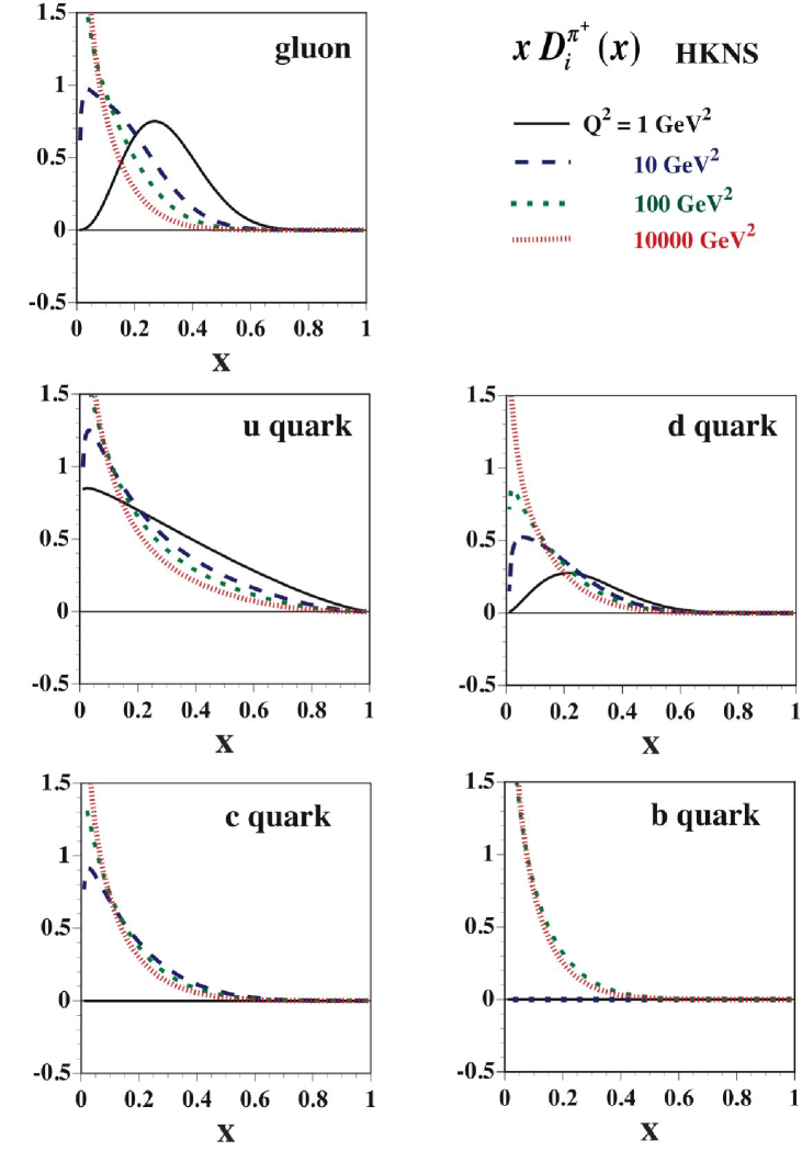
Figure 1: $Q^{2}$ evolution of HKNS07 fragmentation functions. The initial $g$, $u$, and $d$ FFs are supplied at the scale $Q_{0}^{2}$=1 GeV², and the $c$ and $b$ functions are at $m_{c}^{2}$ and $b_{b}^{2}$. They are evolved to the scale $Q^{2}$=10, 100, and 10000 GeV² by the time-like DGLAP evolution equations in the NLO ($\overline{MS}$) by using the code developed in this work. The explicit parameter values are listed in Eq. (14).

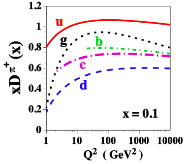
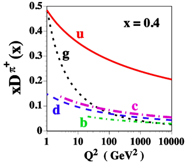
Figure 2: $Q^{2}$ dependence of the fragmentation functions at fiexed $x$ ($=0.1$ and 0.4) . The initial $g$, $u$, and $d$ FFs are supplied at the scale $Q_{0}^{2}$=1 GeV², and the $c$ and $b$ functions are at $m_{c}^{2}$ and $b_{b}^{2}$. They are evolved to the scale $Q^{2}$=10000 GeV² by the time-like DGLAP evolution equations in the NLO ($\overline{MS}$) by using the code developed in this work. The explicit parameter values are listed in Eq. (14).

The input file setup.ini for calculating the evolution of the NLO HKNS07 functions is given in Eq. (14). The light-parton ($g$, $u$, $d$, $s$, $\bar{u}$, $\bar{d}$, $\bar{s}$) FFs are supplied at the initial scale $Q_{0}^{2}$, which is assigned to be the $Q^{2}$ minimum $Q^{2}_{min}$. The evolved $Q^{2}$ value (10, 100, or 10000 GeV²) needs to be supplied when running the code, for example, sample.f.

Next, evolution results are shown by varying the parameters $N_{GL}$, $N_{x}$, and $N_{t}$, which affect the evolution accuracy. First, the $Q^{2}$ evolution results are calculated at $Q^{2}$=100 GeV² by using the HKNS07 parametrization for the initial functions and the parameters $N_{GL}$=100, $N_{x}$=500, and $N_{t}$=500. Then, they are considered to be “standard” functions in showing ratios with other evolution results. In the input setup.ini file, $Q^{2}_{max}$=100 GeV² is taken because the larger-$Q^{2}$ region is not necessary.

First, $N_{GL}$ is varied as 10, 20, and 40 in order to find its dependence on evolution results in checking evolution accuracy. The evolved functions are then used for calculating ratios with the standard evolution by $D_{i}^{\pi^{+}}(x,Q^{2}=100\text{ GeV}^{2})_{N_{GL},N_{x}=500,N_{t}=500}/D_{i}^{\pi^{+}}(x,Q^{2}=100\text{ GeV}^{2})_{N_{GL}=100,N_{x}=500,N_{t}=500}$. The ratios are shown in Fig. 3 for the fragmentation functions of $g$, $u$, $d$, $c$, and $b$. The quark functions are evolved accurately except for the region close to $x=1$ even with a small number of Gauss-Legendre points such as $N_{GL}=10$. However, the gluon evolution depends much on the choice of $N_{GL}$, and the results indicate that $N_{GL}\geq 20$ needs to be taken for getting the evolution accuracy better than about 0.3%. This is the reason why $NGLI=32$ is used in calculating the evolutions in Fig. 1.

Second, the dependence on $N_{x}$ is shown by fixing the other parameters at $N_{GL}$=100 and $N_{t}$=500. The evolved functions are used for taking ratios with the standard evolution results with $N_{GL}$=100, $N_{x}$=500, and $N_{t}$=500 in the same way with Fig. 3. The input parameter $N_{x}$ is the number of points in $x$ from $x_{min}$ to one. For example, if $x_{min}$=0.01 and $N_{x}$=500 are taken, 250 points are given for the logarithmic $x$ in the region $0.01\leq x\leq 0.1$ and another 250 points for the linear $x$ in $0.1\leq x\leq 1$. If $x_{min}$=0.001 and $N_{x}$=600 are taken, we have 400 (200) points in $0.001\leq x\leq 0.1$ ($0.1\leq x\leq 1$). It is changed as $N_{x}$=20, 50, and 200 to show variations in the evolved functions, and results are shown in Fig. 4. In general, there are large differences in the large-$x$ region in all the FFs. In particular, the evolved functions are not reliable at $x>0.7$ if $N_{x}$=20 is taken. As the number increases as $N_{x}$=50 and 200, they become reliable except for the extremely large-$x$ region ($x>0.9$). From these studies, $N_{x}$=160 is taken, for example, in Fig. 1 as a reasonable choice.

Third, we show $N_{t}$ dependence in Fig. 5. It is varied as $N_{t}$=100, 200, and 300 by fixing other parameters at $N_{GL}=100$ and $N_{x}=500$. If $N_{t}$ is small, evolved distributions are not accurate at large $x$, especially in the gluon fragmentation function. A large number of points should be taken for $N_{t}$ for getting a converging function within a few percent level of accuracy, and $N_{t}$=580 is taken in Fig. 1. However, if $Q^{2}_{max}$ is small, accurate evolution results can be obtained by taking smaller $N_{t}$.

A typical running time for obtaining the evolutions in Fig. 1 is 4 seconds by using g95 on the CPU (Dual-Core Intel Xeon 2.66 GHz) with Mac-OSX-10.5.8, so that the code is efficient enough to be used on any machines for one’s studies on the fragmentation functions.

Figure 3: Evolved fragmentation-function ratios $D_{i}^{\pi^{+}}(x)_{N_{GL},\ N_{x}=500,\ N_{t}=500}/D_{i}^{\pi^{+}}(x)_{N_{GL}=100,\ N_{x}=500,\ N_{t}=500}$ are shown for $N_{GL}$=10, 20, and 50 at $Q^{2}$=100 GeV². The initial functions are the HKNS07 ones at $Q^{2}$=1 GeV² for $g$, $u$, and $d$, at $Q^{2}=m_{c}^{2}$ for $c$, and at $Q^{2}=m_{b}^{2}$ for $b$.

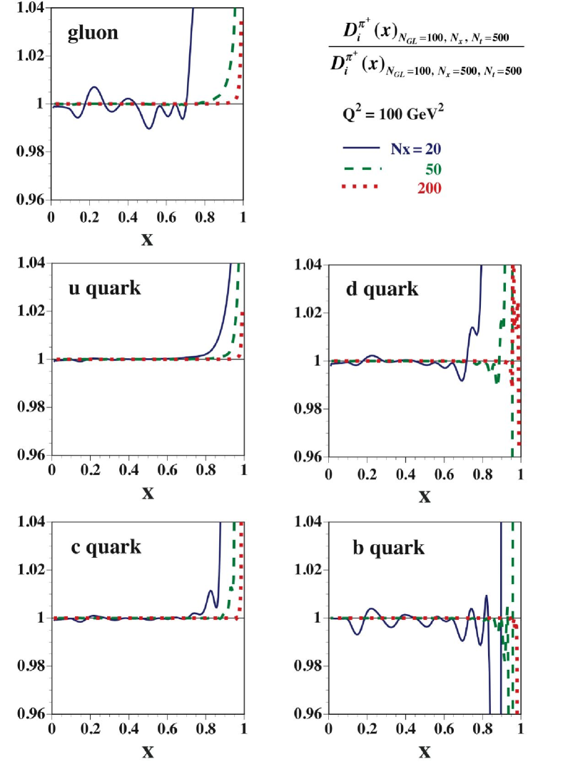
Figure 4: Evolved fragmentation-function ratios $D_{i}^{\pi^{+}}(x)_{N_{GL}=100,\ N_{x},\ N_{t}=500}/D_{i}^{\pi^{+}}(x)_{N_{GL}=100,\ N_{x}=500,\ N_{t}=500}$ are shown for $N_{x}$=20, 50, and 200 at $Q^{2}$=100 GeV². The other conditions are the same as the ones in Fig. 3.

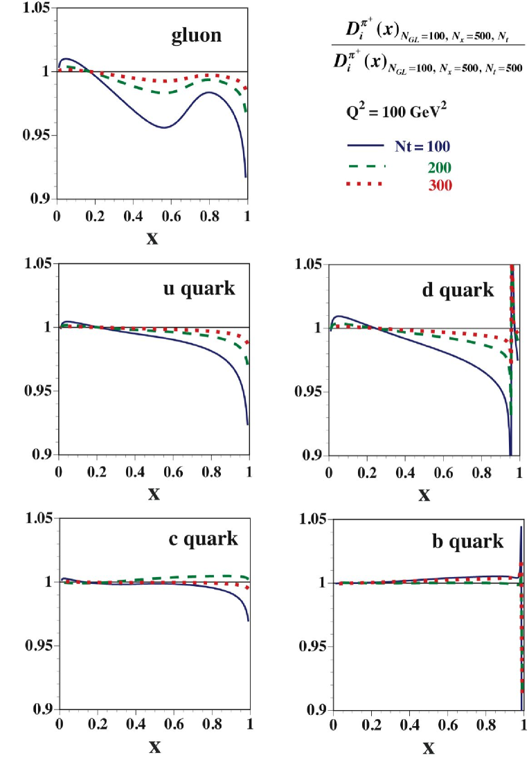
Figure 5: Evolved fragmentation-function ratios $D_{i}^{\pi^{+}}(x)_{N_{GL}=100,\ N_{x}=500,\ N_{t}}/D_{i}^{\pi^{+}}(x)_{N_{GL}=100,\ N_{x}=500,\ N_{t}=500}$ are shown for $N_{x}$=100, 200, and 300 at $Q^{2}$=100 GeV². The other conditions are the same as the ones in Fig. 3.

7 Summary

The fragmentation functions are used in describing hadron-production cross sections at high energies. The FFs are described by two variables $x$ and $Q^{2}$. The $Q^{2}$ dependence of the FFs is calculated in perturbative QCD and they are described by the DGLAP evolution equations. In this work, the $Q^{2}$ evolution equations are numerically solved and a useful evolution code is provided so that other researchers could use it for their own studies. The variables $x$ and $\ln Q^{2}$ are divided into small steps, and the evolution is numerically calculated by using the Euler method and the Gauss-Legendre quadrature. We showed that the evolution is accurately calculated except for the extremely large-$x$ region by taking reasonably large numbers of the Gauss-Legendre points ($N_{GL}$), $x$ steps ($N_{x}$), and $t=\ln Q^{2}$ steps ($N_{t}$). Our evolution code can be obtained upon request request for using one’s studies on the $Q^{2}$ evolution of the FFs.

Appendix A. Running coupling constant

The running coupling constants in the leading order (LO) and next-to-leading order (NLO) are

$$\alpha_{s}^{LO}(Q^{2}) =\frac{4\pi}{\beta_{0}\ln(Q^{2}/\Lambda^{2})},$$ (16)

$$\alpha_{s}^{NLO}(Q^{2}) =\frac{4\pi}{\beta_{0}\ln(Q^{2}/\Lambda^{2})}\Biggl{[}1-\frac{\beta_{1}\ln\ln(Q^{2}/\Lambda^{2})}{\beta_{0}^{2}\ln(Q^{2}/\Lambda^{2})}\Biggr{]},$$ (17)

where $\Lambda$ is the QCD scale parameter, and $\beta_{0}$ and $\beta_{1}$ are given by

$$\beta_{0}={11\over 3}C_{G}-{4\over 3}T_{R}N_{f},\ \ \ \beta_{1}={34\over 3}C^{2}_{G}-{10\over 3}C_{G}N_{f}-2C_{F}N_{f},$$ (18)

with the color constants

$$C_{A}=N_{c},\ \ \ C_{F}=\frac{N_{c}^{2}-1}{2N_{c}},\ \ \ T_{R}=\frac{1}{2}.$$ (19)

In the NLO, $\overline{MS}$ is used for the renormalization scheme.

Appendix B. Splitting functions

The splitting functions are expanded in $\alpha_{s}$:

$$P_{ij}(x,\alpha_{s})=P_{ij}^{(0)}(x)+\frac{\alpha_{s}(Q^{2})}{2\pi}P_{ij}^{(1)}(x)+\cdot\cdot\cdot,$$ (20)

where $P_{ij}^{(0)}(x)$ and $P_{ij}^{(1)}(x)$ are LO and NLO splitting functions, respectively. Splitting functions in the LO are the same as the ones for describing the PDF evolution bfevol :

$$P_{q_{i}q_{j}}^{(0)}(x) =\delta_{ij}C_{F}\ \left[\ {{1+x^{2}}\over{(1-x)_{+}}}\ +\ {3\over 2}\ \delta(1-x)\ \right],$$ (21)

$$P_{qg}^{(0)}(x) =T_{R}\left[\ x^{2}\ +\ (1-x)^{2}\ \right],$$ (22)

$$P_{gq}^{(0)}(x) =C_{F}\ {{1+(1-x)^{2}}\over x},$$ (23)

$$P_{gg}^{(0)}(x) =2C_{G}\left[\ {x\over{(1-x)_{+}}}\ +\ {{1-x}\over x}\ +\ x(1-x)\ +\ \left({{11}\over{12}}-{1\over 3}{{N_{f}T_{R}}\over{C_{G}}}\right)\ \delta(1-x)\ \right].$$ (24)

The only point one should note is that the splitting functions $P_{qg}$ and $P_{gq}$ are interchanged in the matrix of Eq. (8) from the PDF evolution. However, the spacelike and timelike splitting functions for the PDFs and FFs, respectively, are different in higher-order of $\alpha_{s}$ as shown in Refs. esw-book ; splitting . The quark-quark splitting function in the NLO is given by

$$P_{q_{i}^{+}q_{j}^{+}}^{(1)} \equiv P_{q_{i}q_{j}}^{(1)}+P_{q_{i}\bar{q}_{j}}^{(1)}=\delta_{ij}(P_{qq}^{V(1)}+P_{q\bar{q}}^{V(1)})+P_{qq}^{S(1)}+P_{q\bar{q}}^{S(1)},$$ (25)

where the functions $P_{qq}^{V(1)}$ and $P_{q\bar{q}}^{V(1)}$ are given in Ref. esw-book , the function $P_{qq}^{S(1)}$ ($=P_{q\bar{q}}^{S(1)}$) can be derived from the relation $P_{qq}^{(1)}=P_{qq}^{V(1)}+P_{q\bar{q}}^{V(1)}+N_{f}(P_{qq}^{S(1)}+P_{q\bar{q}}^{S(1)})$. These expressions are lengthy and they are provided in Sec. 6.1 of Ref. esw-book .

sample.f

C ---------------------------------------------------------------------
      PROGRAM SAMPLE                                      ! 2011-11-24
C ---------------------------------------------------------------------
C X DEPENDENCE OF FFs
      IMPLICIT REAL*8(A-H,O-Z)
      PARAMETER(NSTEP=200)
      CHARACTER*1 Q2PROG_END
      CHARACTER*9 Q2_OUT
      CHARACTER*22 FNAME
      DIMENSION FF(-5:5),Z(600)
      COMMON /XMIN/XMIN  ! Setting in the setup.ini

      CALL FF_DGLAP() ! Making arrary of FF(XMIN:1.D0, Q2_ini:Q2_max)

200   WRITE(*,fmt=’(a)’) "Q^2= "; READ(*,*) Q2
      WRITE(Q2_OUT,’(1PE9.3)’) Q2
      FNAME=’Q2=’//Q2_OUT//’_GeV2.dat’
      OPEN(unit=23,file=FNAME,FORM=’formatted’)

      DLMIN=DLOG10(XMIN)
      ZLSTEP=(DLOG10(1.D0)-DLMIN)/DFLOAT(NSTEP)
      DO I=1,NSTEP+1
        DLOGZ=DFLOAT(I-1)*ZLSTEP+DLMIN
        Z(I)=10.D0**(DLOGZ)
      END DO

C FOR pi^+, FF(I), I= 0:g, 1:d, 2:u, 3:s, 4:c, 5:b
      DO I=1,NSTEP
        CALL GETFF(Q2,Z(I),FF) ! Getting FF(Z,Q^2)
        WRITE(23,1010) Z(I), Z(I)*FF(0), ! gluon
     +                       Z(I)*FF(2), ! up
     +                       Z(I)*FF(1), ! down
     +                       Z(I)*FF(3), ! strange
     +                       Z(I)*FF(4), ! charm
     +                       Z(I)*FF(5)  ! bottom
      END DO
      WRITE(*,fmt=’(a)’)
     +      "Do you finish the FF Q2 evolution ? (y/n) "
      READ(*,*) Q2PROG_END
      IF((Q2PROG_END(1:1).EQ.’n’).OR.(Q2PROG_END(1:1).EQ.’N’)) GOTO 200

 1010 FORMAT(1X,9(1PE16.7))
      CLOSE(23)
      END
C ---------------------------------------------------------------------

TEST RUN OUTPUT

Running the distributed sample code (sample.f) together with the main $Q^{2}$ evolution subroutine (FF_DGLAP.f) and the input file (setup.ini), we obtain the following output for $Q^{2}$=100 GeV². The following functions corresponds to the curves at $Q^{2}$=100 GeV² in Fig. 1.

$x$	$x\,D_{g}^{\pi^{+}}$	$x\,D_{u}^{\pi^{+}}$	$x\,D_{d}^{\pi^{+}}$	$x\,D_{s}^{\pi^{+}}$	$x\,D_{c}^{\pi^{+}}$	$x\,D_{b}^{\pi^{+}}$
1.0000000E-02	1.7387272E+00	1.5206099E+00	7.1337454E-01	7.1374282E-01	1.2897181E+00	2.5241504E+00
1.0232930E-02	1.7469241E+00	1.5297365E+00	7.2321764E-01	7.2358058E-01	1.2947968E+00	2.5089220E+00
1.0471285E-02	1.7544533E+00	1.5384281E+00	7.3265629E-01	7.3301393E-01	1.2995278E+00	2.4936096E+00
1.0715193E-02	1.7613271E+00	1.5466907E+00	7.4169702E-01	7.4204939E-01	1.3039165E+00	2.4782151E+00
1.0964782E-02	1.7675595E+00	1.5545311E+00	7.5034733E-01	7.5069444E-01	1.3079690E+00	2.4627404E+00
1.1220185E-02	1.7731631E+00	1.5619553E+00	7.5861384E-01	7.5895574E-01	1.3116905E+00	2.4471874E+00
1.1481536E-02	1.7781510E+00	1.5689699E+00	7.6650367E-01	7.6684037E-01	1.3150869E+00	2.4315579E+00
1.1748976E-02	1.7825365E+00	1.5755812E+00	7.7402396E-01	7.7435550E-01	1.3181639E+00	2.4158538E+00
1.2022644E-02	1.7863321E+00	1.5817955E+00	7.8118145E-01	7.8150786E-01	1.3209270E+00	2.4000771E+00
1.2302688E-02	1.7895498E+00	1.5876182E+00	7.8798236E-01	7.8830368E-01	1.3233809E+00	2.3842291E+00
$\cdot\cdot\cdot$	$\cdot\cdot\cdot$	$\cdot\cdot\cdot$	$\cdot\cdot\cdot$	$\cdot\cdot\cdot$	$\cdot\cdot\cdot$	$\cdot\cdot\cdot$
$\cdot\cdot\cdot$	$\cdot\cdot\cdot$	$\cdot\cdot\cdot$	$\cdot\cdot\cdot$	$\cdot\cdot\cdot$	$\cdot\cdot\cdot$	$\cdot\cdot\cdot$
$\cdot\cdot\cdot$	$\cdot\cdot\cdot$	$\cdot\cdot\cdot$	$\cdot\cdot\cdot$	$\cdot\cdot\cdot$	$\cdot\cdot\cdot$	$\cdot\cdot\cdot$
8.9125094E-01	2.7586761E-05	7.8509439E-03	1.0318809E-06	1.0318809E-06	4.2783416E-05	1.7161909E-06
9.1201084E-01	1.4513488E-05	5.0877079E-03	2.3777347E-07	2.3777347E-07	1.6972984E-05	4.9828819E-07
9.3325430E-01	6.3142094E-06	2.8910396E-03	3.2396330E-08	3.2396330E-08	5.0850503E-06	9.9610221E-08
9.5499259E-01	1.9415364E-06	1.2925565E-03	7.2014456E-10	7.2014458E-10	9.1254976E-07	1.0039050E-08
9.7723722E-01	2.5705072E-07	3.2218983E-04	$-$2.2238409E-10	$-$2.2238409E-10	4.7361837E-08	1.7555729E-10

References

- (1) B. A. Kniehl, G. Kramer, and B. Pötter, Nucl. Phys. B 582 (2000) 514; S. Kretzer, Phys. Rev. D 62 (2000) 054001; S. Albino, B. A. Kniehl, and G. Kramer, Nucl. Phys. B 725 (2005) 181; B. A. Kniehl and G. Kramer, Phys. Rev. D 74 (2006) 037502.
- (2) M. Hirai, S. Kumano, T.-H. Nagai, and K. Sudoh, Phys. Rev. D 75 (2007) 094009. A code for the HKNS07 fragmentation functions is provided at http://research.kek.jp/people/kumanos/ffs.html.
- (3) M. Hirai, S. Kumano, M. Oka, and K. Sudoh, Phys. Rev. D 77 (2008) 017504.
- (4) D. de Florian, R. Sassot, and M. Stratmann, Phys. Rev. D 75 (2007) 114010; 76 (2007) 074033; T. Kneesch, B. A. Kniehl, G. Kramer, and I. Schienbein, Nucl. Phys. B 799 (2008) 34; S. Albino, B. A. Kniehl, and G. Kramer, Nucl. Phys. B 803 (2008) 42; E. Christova and E. Leader, Phys. Rev. D 79 (2009) 014019; S. Albino and E. Christova, Phys. Rev. D 81 (2010) 094031.
- (5) S. Albino et al., arXiv:0804.2021 [hep-ph]; F. Arleo, Eur. Phys. J. C 61 (2009) 603; F. Arleo and J. Guillet, online generator of FFs at http://lapth.in2p3.fr/generators/ .
- (6) M. Glück, P. Jimenez-Delgado, and E. Reya, Eur. Phys. J. C53 (2008) 355; A. D. Martin, W. J. Stirling, R. S. Thorne, and G. Watt, Eur. Phys. J. C63 (2009) 189; S. Alekhin, J. Blümlein, S. Klein, and S. Moch, Phys. Rev. D 81 (2010) 014032; H.-L. Lai et al., Phys. Rev. D82 (2010) 074024.
- (7) AAC (Asymmetry Analysis Collaboration), Y. Goto et al., Phys. Rev. D 62 (2000) 034017; M. Hirai, S. Kumano, and N. Saito, Phys. Rev. D 69 (2004) 054021; 74 (2006) 014015; M. Hirai and S. Kumano, Nucl. Phys. B 813 (2009) 106.
- (8) D. de Florian, R. Sassot, M. Stratmann, and W. Vogelsang, Phys. Rev. D 80 (2009) 034030; J. Blümlein and H. Böttcher Nucl. Phys. B 841 (2010) 205; E. Leader, A. V. Sidorov, and D. B. Stamenov, Phys. Rev. D 82 (2010) 114018; arXiv:1103.5979 [hep-ph].
- (9) M. Hirai, S. Kumano, and M. Miyama, Phys. Rev. D 64 (2001) 034003; M. Hirai, S. Kumano, and T.-H. Nagai, Phys. Rev. C 70 (2004) 044905; 76 (2007) 065207.
- (10) D. de Florian and R. Sassot, Phys. Rev. D 69 (2004) 074028; K. J. Eskola, H. Paukkunen, and C. A. Salgado, JHEP 04 (2009) 065; I. Schienbein, J. Y. Yu, C. Keppel, J. G. Morfin, F. I. Olness, and J. F. Owens, Phys. Rev. D 77 (2008) 054013; D80 (2009) 094004. See also L. Frankfurt, V. Guzey, and M. Strikman, Phys. Rev. D 71 (2005) 054001; V. Guzey and M. Strikman, Phys. Lett. B687 (2010) 167; S. A. Kulagin and R. Petti, Phys. Rev. D 76 (2007) 094023.
- (11) V. N. Gribov and L. N. Lipatov, Sov. J. Nucl. Phys. 15 (1972) 438 and 675; G. Altarelli and G. Parisi, Nucl. Phys. B126 (1977) 298; Yu. L. Dokshitzer, Sov. Phys. JETP 46 (1977) 641.
- (12) M. Glück, E. Reya, and A. Vogt, Z. Phys. C48 (1990) 471; D. Graudenz, M. Hampel, A. Vogt, and C. Berger, Z. Phys. C70 (1996) 77; J. Blümlein and A. Vogt, Phys. Rev. D58 (1998) 014020; J. Blümlein, Comput. Phys. Commun. 133 (2000) 76; M. Stratmann and W. Vogelsang, Phys. Rev. D64, 114007 (2001).
- (13) M. Miyama and S. Kumano, Comput. Phys. Commun. 94 (1996) 185; M. Hirai, S. Kumano, and M. Miyama, Comput. Phys. Commun. 108 (1998) 38. See http://research.kek.jp/people/kumanos/program.html.
- (14) M. Hirai, S. Kumano, and M. Miyama, Comput. Phys. Commun. 111 (1998) 150.
- (15) W. Furmanski and R. Petronzio, Nucl. Phys. B195 (1982) 237; G. P. Ramsey, J. Comput. Phys. 60 (1985) 97; J. Blümlein, G. Ingelman, M. Klein, and R. Rückl, Z. Phys. C45 (1990) 501; S. Kumano and J. T. Londergan, Comput. Phys. Commun. 69 (1992) 373; R. Kobayashi, M. Konuma, and S. Kumano, Comput. Phys. Commun. 86 (1995) 264.
- (16) S. Kumano and T.-H. Nagai, J. Comput. Phys. 201 (2004) 651.
- (17) For example, see K. J. Golec-Biernat, S. Jadach, W. Placzek, and M. Skrzypek, Acta Phys. Polon. B37 (2006) 1785; M. M. Block, L. Durand, P. Ha, and D. W. McKay, Eur. Phys.J. C69 (2010) 425 and references therein.
- (18) T. Ito, W. Bentz, I. C. Cloet, A. W. Thomas, and K. Yazaki, Phys. Rev. D 80 (2009) 074008; H. H. Matevosyan, A. W. Thomas, and W. Bentz, Phys. Rev. D 83 (2011) 074003.
- (19) R. K. Ellis, W. J. Stirling, and B. R. Webber, QCD and Collider Physics (Cambridge University Press, 1996).
- (20) P. Nason and B. R. Webber, Nucl. Phys. B 421 (1994) 473; Erratum, ibid. 480 (1996) 755. See also G. Altarelli, R. K. Ellis, G. Martinelli, and S.-Y. Pi, Nucl. Phys. B 160 (1979) 301; W. Furmanski and R. Petronzio, Z. Phys. C 11 (1982) 293; A. Mitov and S. Moch, Nucl. Phys. B 751 (2006) 18.
- (21) J. Collins, Nucl. Phys. B 396 (1993) 161; G. Sterman et al., Rev. Mod. Phys. 67 (1995) 157.
- (22) M. Stratmann and W. Vogelsang, Nucl. Phys. B 496 (1997) 41. NNLO results are in A. Mitov, S. Moch, and A. Vogt, Phys. Lett. B 638 (2006) 61.
- (23) B. Carnahan, H. A. Luther, and J. O. Wilkes, Applied Numerical Methods (John Wiley & Sons, 1969).
- (24) W. H. Press et al., Numerical Recipes: The Art of Scientific Computing, Third edition (Cambridge University Press, 2007), pp. 179-188.
- (25) If one is interested in obtaining the evolution code of the fragmentation functions, please send an email message to M. Hirai and S. Kumano (mhirai@ph.noda.tus.ac.jp, shunzo.kumano@kek.jp) as instructed in http://research.kek.jp/people/kumanos/program.html .
- (26) pp.98-99 in R. G. Roberts, The Structure of the Proton (Cambridge University Press, Cambridge, 1990).
- (27) M. Stratmann, personal communication on grid points around the threshould point (2011).
- (28) S. Albino, B. A. Kniehl, and G. Kramer, Eur. Phys. J. C38 (2004) 177.