Momentum transport and torque scaling in Taylor-Couette flow from an analogy with turbulent convection

Abstract

We generalize an analogy between rotating and stratified shear flows. This analogy is summarized in Table 1. We use this analogy in the unstable case (centrifugally unstable flow v.s. convection) to compute the torque in Taylor-Couette configuration, as a function of the Reynolds number. At low Reynolds numbers, when most of the dissipation comes from the mean flow, we predict that the non-dimensional torque $G=T/\nu^{2}L$, where $L$ is the cylinder length, scales with Reynolds number $R$ and gap width $\eta$, $G=1.46\eta^{3/2}(1-\eta)^{-7/4}R^{3/2}$. At larger Reynolds number, velocity fluctuations become non-negligible in the dissipation. In these regimes, there is no exact power law dependence the torque versus Reynolds. Instead, we obtain logarithmic corrections to the classical ultra-hard (exponent $2$) regimes:

$$G=0.50\frac{\eta^{2}}{(1-\eta)^{3/2}}\frac{R^{2}}{\ln[\eta^{2}(1-\eta)R^{2}/10^{4}]^{3/2}}.$$

These predictions are found to be in excellent agreement with available experimental data. Predictions for scaling of velocity fluctuations are also provided.

I Motivation and objectives

At sufficiently large Reynolds number, the fluid between co-rotating coaxial cylinders becomes turbulent, and a significant momentum transport occurs between the two cylinders. In the case with rotating inner cylinder and resting outer one (the so-called Taylor-Couette flow), detailed measurements show that the torque applied at cylinders by the turbulent flow is a function of the Reynolds number $R$. There is no clear consensus about this dependence yet: marginal stability computation of King et al KLSM84 or Barcilon and Brindley BarcBrin84 predict that the non-dimensional torque $G=T/\nu^{2}L$, where $L$ is the cylinder height should vary like $G\sim R^{5/3}$. Old experimental data indicated the existence of two scaling regimes, one for $R>10^{4}$ where the exponent is $1.5$, and one for larger Reynolds number, where the exponent switches towards $1.7-1.8$ Wendt33 ; Taylor36 ; TGHW90 . Recent high precision experimental data yielded no region of constant exponent, and revealed a transition with a marked change of approximate slope of $G$ as a function of $R$ LFS92 ; LewiSwin99 . This observation led Eckhardt et al EGL00 to propose a new theory, in which the dependence $G$ versus $R$ is through a superposition of scaling laws (describing contribution from a boundary layer and the bulk flow). They claim that this superposition fits the data better than the Prandtl-Karman skin friction law proposed by Pant92 ; LFS92 ; LewiSwin99 . Note that all the scalings are within the theoretical bound derived by Doering and Constantin DoerConst92 , which implies that the non-dimensional torque cannot increase faster than $R^{2}$.

The observational features are reminiscent of heat transport in turbulent thermal convection, where approximate scaling laws and transition between different regimes have also been observed (for a review see GrosLohs00 ). In fact, this similarity is pointed out in LFS92 , and in EGL00 , and similar techniques are used in MalkVero58 ; KLSM84 and in GrosLohs00 ; EGL00 to derive theoretically the scaling regimes in the Rayleigh-Bénard system, and in the Taylor-Couette system. However, the similarity is more than superficial: as well known since several decades Brad69 , there is an exact analogy between equations of motions of rotating and stratified shear flows (stable or not). There must therefore exist an exact analogy between the momentum and heat transport in these two systems, although it has so far never been explored. Our goal here is to derive this analogy, and examine its consequences in the unstable regime, where the angular momentum or temperature stratification leads to a linear instability. We thus in this paper mainly focus on the analogy between centrifugally unstable Taylor-Couette flow, and convection.

II The analogy

II.1 Reminder

The root of the analogy can be found in the Lamb formulation of the Navier-Stokes equations:

$$\partial_{t}{\bf u}-{\bf u}\times{\bf\omega}=-\nabla\left(p+\frac{u^{2}}{2}\right)+\nu\Delta{\bf u},$$ (1)

where ${\bf\omega}$ is the vorticity, $p$ is the pressure and $\nu$ the molecular viscosity. The constant density has been set equal to one for simplicity. In a rotating shear flow ${\bf u}=V(r){\bf e_{\theta}}$, the vorticity is only in the axial direction and the Lamb vector ${\bf u}\times{\bf\omega}$ acts only in the radial direction. Its contribution can be split in two parts:

$${\bf e_{r}}\cdot({\bf u}\times{\bf\omega})=VS+2\frac{\Omega}{r}{\cal L},$$ (2)

where ${\cal L}=rV$ is the angular momentum, $\Omega=V/r$ is the angular velocity and $S=r\partial_{r}\Omega$ is the shear. The first contribution is the exact analog of the Lamb vector of a pure shear flow, in a plane parallel geometry. The second contribution reflects the stabilizing influence of the Coriolis force. Its analog would be produced by temperature stratification in the spanwise direction of a planar shear flow. The equation of angular momentum conservation then suggests to split further this analogy by requiring that $2\Omega/r\sim\beta g$, where $g$ is the gravity, and $\beta$ a coefficient of thermal expansion, and ${\cal L}\sim\Theta$, the potential temperature. This remark is at the heart of the analogy between the stability properties of rotating and stratified shear flows, and has been used in the past (see e.g. Brad69 …). Our point here is to show that it can be extended into the turbulent regime, via a new Langevin model of small-scale turbulence. This new model is based on Rapid Distorsion Theory, i.e. on linearized equations for the small-scale motions. This linear structure explains the possibility of extension of the analogy towards the turbulent regime.

II.2 The turbulent model

The turbulent model has been described and tested in LDN01 for general 3D flows, in NKD00 ; DLNK01 for shear flows and in DLSW02 ; DLS02 ; Dubr00 ; Dubr01 for stratified shear flows. In this model, the dynamics of the turbulent flow is obtained from solutions of two coupled sets of equations. The first one described the dynamics of the mean velocity ${\bf U}$:

$$\partial_{t}U_{i}+\partial_{j}U_{i}U_{j}+\partial_{j}<u_{i}^{\prime}u_{j}^{\prime}>=-\partial_{i}P+\nu\partial_{j}\partial_{j}U_{i},$$ (3)

Here, the primes denote fluctuating quantities and $<>$ the averaging. To close the system, we need $<u_{i}^{\prime}u_{j}^{\prime}>$. They are obtained as solution of a linear, stochastic equation valid for localized wave-packets of velocity and temperature:

$$D_{t}\hat{u}_{i} = -ik_{i}\hat{p}-\hat{u}_{j}\partial_{j}U_{i}-\nu_{t}k^{2}\hat{u}_{i}+\hat{f}_{i}$$

$$k_{i}\hat{u}_{i} = 0,$$ (4)

where

$${\hat{u}}({\bf x},{\bf k},t)=\int g(|{\bf x-x^{\prime}}|)e^{i{\bf k\cdot(x-x^{\prime})}}{\bf u}({\bf x^{\prime}},t)d{\bf x^{\prime}},$$ (5)

$g$ being a function which decreases rapidly at infinity. We have dropped primes on fluctuating quantities for convenient notations and introduced the total derivative $D_{t}=\partial_{t}+U_{j}\partial_{j}-\partial_{j}(U_{i}k_{i})\partial_{k_{j}}$ . Once the solutions of (4) have been computed, the Reynolds stress is found by an inverse Gabor transform as:

$$<u^{\prime}_{i}u^{\prime}_{j}>=\int d{\bf k}\left(u^{\prime}_{i}({\bf k},{\bf x},t)u^{\prime}_{j}(-{\bf k},{\bf x},t)+(u^{\prime}_{i}(-{\bf k},{\bf x},t)u^{\prime}_{j}({\bf k},{\bf x},t)\right).$$ (6)

Note that the linear part of (4) is exact and describes non-local interactions between the mean and the fluctuating part. The major approximation of the model is to lump the non-linear terms describing local interactions between fluctuations into a turbulent viscosity $\nu_{t}$. The force $f$ appearing in (4) is a small scale random forces which is introduced to model the seeding of small scales by energy cascades (for example via turbulent structures, detaching from the wall).

II.3 The Taylor-Couette case

In the Taylor-Couette (rotating shear flow) case, the equations for the azimuthal component of the velocity $V(r)$ simplify into:

$$\partial_{t}V+\frac{1}{r^{2}}\partial_{r}r^{2}<uv>=\nu\left(\nabla^{2}V-\frac{V}{r^{2}}\right).$$ (7)

The equation for the fluctuations $(u,v,w)$ become:

$$D_{t}\hat{u} = 2\frac{k_{r}k_{\theta}}{k^{2}}\left(\Omega+S\right)\hat{u}+2\Omega\hat{v}\left(1-\frac{k_{r}^{2}}{k^{2}}\right)-\nu_{t}k^{2}\hat{u}+\hat{f}_{r},$$

$$D_{t}\hat{v} = 2\frac{k_{\theta}^{2}}{k^{2}}\hat{u}(\Omega+S)-2\frac{k_{r}k_{\theta}}{k^{2}}\hat{v}\Omega-\left(2\Omega+S\right)\hat{u}-\nu_{t}k^{2}\hat{v}+\hat{f}_{\theta},$$

$$D_{t}\hat{w} = 2\frac{k_{\theta}k_{z}}{k^{2}}\hat{u}(\Omega+S)-2\frac{k_{r}k_{z}}{k^{2}}\hat{v}\Omega-\nu_{t}k^{2}\hat{w}+\hat{f}_{z}.$$ (8)

Here, we have used the incompressibility to eliminate the pressure. These equations have to be supplemented by the equations describing the ray trajectories:

$$\dot{r} = 0,\quad\dot{\theta}=\Omega,\quad\dot{z}=0,$$

$$\dot{k_{r}} = -k_{\theta}S,\quad\dot{k_{\theta}}=0,\quad\dot{k_{z}}=0.$$ (9)

We now introduce a pseudo-temperature

$$\hat{\theta}=r(\hat{v}-\frac{k_{\theta}}{k_{z}}\hat{w})=ir\frac{\hat{\omega}_{r}}{k_{z}},$$ (10)

where $\hat{\omega}_{r}$ is the radial vorticity. With this temperature and using the incompressibility condition ${\bf k}\cdot{\bf u}=0$, we can rewrite (8) as:

$$D_{t}\hat{u} = 2S\frac{k_{r}k_{\theta}}{k^{2}}\hat{u}+2\frac{\Omega}{r}\frac{k_{z}^{2}}{k^{2}}\hat{\theta}-\nu_{t}k^{2}\hat{u}+\hat{f}_{r},$$

$$D_{t}\hat{\theta} = (2\Omega+S)r\hat{u}-\nu_{t}k^{2}\hat{\theta}+\hat{f}_{\theta},$$ (11)

The set of equation (LABEL:analogb) is the exact analog of the equations describing the behavior of vertical and temperature fluctuations in a stratified shear flow (see DLSW02 ; DLS02 ; Dubr00 ; Dubr01 for their expression), provided the correspondence summarized in Table 1. holds. Note that the analog of the temperature is not the angular momentum, but related to the z-integral of the radial vorticity (in Gabor variable, integration on z is done via division by $k_{z}$). At large scale, since the velocity profile is axi-symmetric, this integral of the radial vorticity reduces to the angular momentum, as previously suggested Brad69 .

II.4 Stability and Importance of axi-symmetric modes

The correspondence described in Table 1. generalizes the well-known analogy established previously Brad69 for the stability analysis under axi-symmetric perturbations (case where $k_{\theta}=0$). In particular, from (LABEL:analogb), one can write a compact differential equation for $\omega=uk^{2}$ :

$$D_{t}^{2}\omega+\kappa^{2}k_{z}^{2}\frac{\omega}{k^{2}}-\nu k^{2}\omega+f_{\omega}=0,$$ (13)

where $\kappa^{2}=2\Omega(2\Omega+S)$ is the epicyclic frequency. Using the ray equation (9), one can then define a non-dimensional number $B=\kappa^{2}k_{z}^{2}/(k_{\theta}^{2}+k_{z}^{2})$ (the Bradshaw number) which governs the stability of the wave packet along the trajectory. This number is the analog of Richardson number in stratified shear flow. For example, it can be shown that in the absence of diffusion, the amplitude of the wavepacket has a monotonic (growing for one mode, decaying for another one) behavior at late time for $B<1/4$, while it becomes oscillatory for $B>1/4$. Clearly, the oscillatory behavior creates dephasing effects for the Reynolds stresses, which may lead to its pure cancellation, thereby removing the influence of the small scales onto the large scale. We therefore identify the regime with $B>1/4$ as a regime with purely laminar motions, where turbulence effects are strongly suppressed. This property tends to favor bi-dimensional modes (those for which $k_{z}=0$) since in this case the epicyclic frequency can take any value for non-oscillatory behavior. The inclusion of diffusion changes the mode selection. One can indeed check that the viscous decay is proportional to $\exp(-R^{-1}tS)$ rather than $\exp(-R^{-1}(tS)^{3})$ for non-axi-symmetric perturbations. This shows that axi-symmetric perturbation (with $k_{\theta}=0$) are favored with respect to non-axi-symmetric perturbation. In this case, the Bradshaw number becomes independent of the wavenumber of the wave packet, and one can identify a new boundary of stability according to its sign: when it is positive, axi-symmetric perturbations can be exponentially amplified and superseed viscous decay. We call this regime ”unstable”. It is the analog of the convective regime in the stratified case. In the sequel (Section 3), we shall concentrate on this regime, leaving the other regime for further study.

II.5 Completion of the analogy in the unstable case

For axi-symmetric modes, $\omega_{r}/k_{z}=v$ and the equation for the mean angular momentum ${\cal L}$ can then be written in equivalent form:

$$\partial_{t}{\cal L}+\frac{1}{r}\partial_{r}(r<u\theta>)=\nu\left(\nabla^{2}{\cal L}/r-\frac{{\cal L}}{r^{2}}\right).$$ (14)

Comparing this equation with the equation giving the mean temperature profile, we finally remark that the only difference lies in the viscous terms, because in cylindrical coordinates, the Laplacian includes terms describing curvature effects. In the most general case, this forbids the analogy to be drawn at the level on mean profile (ie after integration over $r$ of eq. (7): for example, it is well known that in stratified shear flow, the laminar temperature profile is linear, while its analog, the laminar angular momentum profiles varies like: $L\sim Ar^{2}+B$. In many Taylor-Couette experiments, however, the gap between the two cylinders is small, and curvature effects can be neglected. One can for example check that the angular momentum in the experiments by LFS92 is linear in the laminar regime, while it flattens at the center of the gap in the turbulent regime, exactly like its temperature analog. In the sequel, we shall assume a small gap geometry, and neglect curvature effects.

III Application of the analogy in the unstable case

The present analogy is the turbulent generalization of a previously known analogy for axi-symmetric modes. In the sequel, we shall use previous considerations about stability of axi-symmetric modes to assume that the turbulent properties are dominated by the contribution of the axi-symmetric modes, i.e. restrict ourselves to these modes. The relevence of this approximation will be tested by comparisons of its predictions regarding some characteristic quantities measured, in the turbulent regime with experimental data.

III.1 Stability

In the unstable regime, a classical parameter describing the intensity of the convection is the Rayleigh number:

$$Ra=\frac{\beta gD^{3}\Delta\Theta}{\kappa\nu},$$ (15)

where $D$ is the size of the cell in the stratified direction, $\Delta\Theta$ is the temperature gradient applied. In most convection experiments, this number is unambiguously defined because of the constancy of the gravity at the scale of the experiment. In the Taylor-Couette case, the gravity depends on the perturbation, and one may wonder how to define this Rayleigh number in a general way. In a recent analysis of stability of Taylor-Couette experiment, Esser and Grossman EsseGros96 suggested to evaluate this factor at the gap center, $r_{c}=(r_{1}+r_{2})/2$, leading to

$$Ra_{*} \equiv -2\frac{\Omega}{r}\partial_{r}{\cal L}\frac{d^{4}}{\nu^{2}}|_{r=r_{c}},$$ (16)

$$= 4\frac{\eta^{2}}{(1-\eta^{2})^{2}}\left(\frac{d^{2}}{r_{c}^{2}}-\frac{d^{2}}{r_{2}^{2}}\right)R^{2},$$

$$= 4\frac{\eta^{2}(1-\eta)(3+\eta)}{(1+\eta)^{4}}R^{2}.$$

In the sequel, we shall use a star label to refer to analog quantities. In (16), we have used $\kappa_{*}=\nu$ and introduced the Reynolds number $R=r_{1}d\Omega_{1}/\nu$, where $r_{1}$ is the internal radius, $\Omega_{1}$ the rotation rate at the inner radius, $d$ the gap width and $\eta=r_{1}/r_{2}$. Note that the analog Rayleigh number $Ra_{*}$ varies with the radial aspect ratio $\eta$. In the small gap approximation $\eta\to 1$, experiments show that the critical Rayleigh number tends to a constant $Ra_{*}\approx 1706$. This value is very close to the value $Ra=1707.762$ obtained in Rayleigh-Bénard convection for rigid boundary conditions Chan70 . In sheared convection, the critical Rayleigh number is modified with respect to this theoretical value, and display corrections quadratic in the Reynolds number based on the shear. In the present case, these correction are proportional to $(1-\eta)^{4}\to 0$, and the critical Rayleigh number stays close to the un-sheared value $Ra=1707.762$. A last modification of the critical Rayleigh number occurs because of lateral wall effects. As a result, the critical Rayleigh number increases with decreasing aspect ratio $\Gamma$ (lateral width over radial width). For example, for $\Gamma=5,2,1,0.5$, $Ra_{c}=1779,2013,2585,12113$. In most Taylor-Couette experiments, the aspect ratio is very large (typically above 8 or so). So the analog critical Rayleigh number is close to $1708$. However, many modern convection experiment (reaching very large Rayleigh numbers) deal with a rather small aspect ratio ($\Gamma\sim 1$). This unfortunately limits the possibilities of direct comparisons between the Taylor-Couette experiments and the convective experiments to values close to the onset of instability. For larger values of Rayleigh numbers, we shall use extrapolations.

III.2 Angular momentum transfer

A second interesting quantity in convection is the non-dimensional heat transfer $Nu=Hd/\kappa\Delta T$, where $H$ is the heat transfer. Via the analogy, the analog of this is the non-dimensional angular momentum transfer, which can be computed using the non-dimensional torque $G=T/\nu^{2}L$, where $L$ is the cylinder length:

$$Nu_{*} \equiv \frac{G}{G_{laminar}},$$ (17)

$$= \frac{G}{R}\frac{(1+\eta)(1-\eta)^{2}}{4\pi\eta}.$$

The normalization by $G_{laminar}$ ensures that in the laminar case, $Nu_{*}=1$, like in the convective analog.

III.2.1 Instability onset

Theoretical SLB65 and experimental PlatLegr84 studies of convection near threshold lead to identification of two regimes just above the critical Rayleigh number:

for $\epsilon=\frac{Ra-Ra_{c}}{Ra_{c}}\leq 1$, a linear regime in which

$$\left(Nu-1\right)\frac{Ra}{Ra_{c}}=K_{1}\epsilon.$$ (18)

The constant $K_{1}$ depends on the Prandtl number. For $Pr=1$, it is $K_{1}\approx 1/0.7=1.43$ SLB65 .

for larger $\epsilon$, a scaling regime in which PlatLegr84

$$\left(Nu-1\right)\frac{Ra}{Ra_{c}}=K_{2}\epsilon^{1.23}.$$ (19)

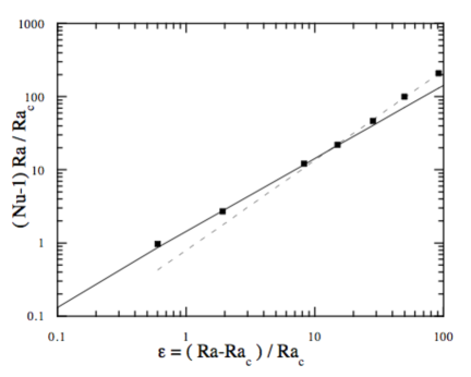
Here, $K_{2}$ is a constant which is not predicted by the theory. In Fig. 1, we show how the results of Wendt obtained with $\eta=0.935$ near the instability threshold compare with these two predictions. One sees that the linear regime is indeed obtained for $\epsilon\leq 10$, while the scaling regime is obtained for larger values of $10<\epsilon<100$. Further from the threshold, one needs to compare with the turbulent theories of convection.

Figure 1: Comparison of the theoretical near instability onset behavior with the data of Wendt Wendt33 . The symbols are the experimental measurements. The two lines are the theoretical formula predicted by analogy with convection for $\epsilon<1$ ($(Nu-1)Ra/Ra_{c}=1.43\epsilon$ and for $\epsilon>1$ ($(Nu-1)Ra/Ra_{c}\sim\epsilon^{1.23}$.) In the latter case, the proportionality constant is not constrained by the analogy, and needs to be adjusted for a best fit.

III.3 The classical turbulent regimes

Using (17), we can single out some interesting regimes. Note that since $\kappa_{*}=\nu$, we are in the case of unit Prandtl number convection, i.e. for example convection in Helium ($Pr>0.7$). In the classical theory of convection, one usually considers three regimes: a first one, labeled as ”soft turbulence”, in which $Nu\sim Ra^{1/3}$, $5\times 10^{5}<Ra<2\times 10^{7}$ HCL87 ; then for $2\times 10^{7}<Ra<10^{11}$, a ”hard turbulence” regimes in which $Nu\sim Ra^{2/7}$ Cast89 ; finally for $Ra>10^{11}$, a ultra-hard turbulence regime in which $Nu\sim Ra^{1/2}$ Krai62 ; CCCHCC97 . Using the analogy, we see that these three regimes translate into: for $707<R\eta(1-\eta)^{1/2}<4472$, $G\sim R^{5/3}$; for $4472<R\eta(1-\eta)^{1/2}<3\times 10^{5}$, $G\sim R^{11/7}$; for $(1-\eta)^{1/2}\eta R>3\times 10^{5}$, $G\sim R^{2}$. To evaluate the boundary between the two regimes, we have used (16) at $\eta=1$.

The first regime has been predicted by KLSM84 ; BarcBrin84 using marginal stability analysis. The third regime can be derived from Kolmogorov type arguments (see e.g. LFS92 ). It also corresponds to some upper-bound in the angular momentum transport DoerConst92 . The intermediate regime is new, and leads to a scaling exponent of $1.57$. Experimentally, some of this scaling regimes have been reported, but not in the same sequence: in his experiments with $0.680<\eta<0.935$, Wendt Wendt33 reports a scaling exponent of $1.5$ for $400<R<10^{4}$, followed by a scaling exponent $1.7$ for $10^{4}<R<10^{5}$. In more recent experiments, Lathrop et al LFS92 measure a “local” exponents $d\ln(G)/d\ln(R)$ which varies continuously from $1.2$ to $1.9$, with a transition at $R\sim 1.3\times 10^{4}$ (for $\eta=0.7246$). This transition was later found to correspond to a modification of coherent structures in the flow LewiSwin99 . Remarkably enough, the analog Rayleigh number characterizing this transition is $Ra_{*}=2\times 10^{7}$, like in convection. We may therefore interpret it as the boundary between ”soft” and ”hard” turbulence. However, the scaling reported in LFS92 does not seem to fully correspond to the soft and hard turbulence scaling. In the sequel, we wish therefore to explore a new possibility, based on logarithmic corrections to scaling.

III.4 The logarithmic turbulent regimes

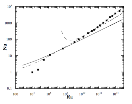
The observation by LFS92 that no scaling prevails for the angular momentum transport has in fact its counter-part for the heat transport in convection GrosLohs00 . In a recent work, we used the turbulent model to analytically compute the heat transport in a convective cell. At $Pr=1$, we found 3 different regimes: at low Rayleigh number, the dissipation is dominated by the mean flow, and $Nu=K_{1}Ra^{1/4}Pr^{-1/12}$; at larger Rayleigh number, the kinetic energy dissipation starts being dominated by velocity fluctuations, and the heat transport becomes $NuPr^{1/9}=K_{2}Ra^{1/3}/\ln(RaPr^{2/3}/20)^{2/3}$. Finally at very large Rayleigh number, the heat dissipation becomes also dominated by (heat) fluctuations, and $Nu=K_{3}Ra^{1/2}/\ln(Ra/Ra_{c})^{3/2}$. Fig. 2 shows the illustration of these 3 regimes in a Helium experiment of CCCHCC97 , with the three fits corresponding to these 3 regimes. From this graph, we obtain $K_{1}=0.31$, $K_{2}=0.45$, $K_{3}=0.023$ and $Ra_{c}=2\times 10^{7}$, for an aspect ratio of $0.5$. These constants tend to decrease slightly for larger aspect ratio by an asymptotic factor of about $0.75$ (at $Ra=10^{8}$, see table 1 of CCCHCC97 ). The small aspect ratio of the experiment also increases the critical Rayleigh for instability from near $1708$ to near $4\times 10^{4}$. The boundary between the regime 1 and 2 lies at $Ra=1.5\times 10^{8}$. It is characterized by a change in the temperature statistics, going from nearly Gaussian to exponential. The boundary between the regime 2 and 3 is somehow ill defined, and lies between $Ra=2\times 10^{10}$ and $Ra=10^{11}$. Note than in a similar experiment, ran by another group, the third regime was not detected, even at $Ra=10^{15}$ NSSD00 . The reason of this difference is not yet known. A possibility would be that different boundary conditions may or may not allow the growth of the temperature perturbation, thereby favoring or inhibiting this last regime Dubr01 .

Figure 2: Illustration of the three scaling regimes found in convection in Helium for Nusselt vs Rayleigh. The symbols are experimental measurements by CCCHCC97 . The lines are theoretical prediction by Dubr01 using an analytical model of turbulent convection. ”Soft” turbulence regime(mean flow dominated): power law $Nu\sim Ra^{1/4}$ (full line); ”Hard” turbulence regime: (velocity fluctuation dominated) $Nu\sim Ra^{1/3}/(\ln(Ra))^{2/3}$ (dotted line); ”Ultra-hard” turbulent regime: (temperature fluctuations dominated) $Nu\sim Ra^{1/2}/(\ln(Ra))^{3/2}$ (dashed line)

The translation of the three logarithmic regimes using the analogy gives a priori three possible regimes in the Taylor-Couette experiments.

In the regime 1, we get:

$$G=K_{4}\frac{\eta^{3/2}}{(1-\eta)^{7/4}}R^{3/2}.$$ (20)

In the regime 2, we get:

$$G=K_{5}\frac{\eta^{2/3}}{(1-\eta)^{5/3}}\frac{R^{5/3}}{\ln[\eta^{2}(1-\eta)R^{2}/K_{6}]^{2/3}},$$ (21)

while in the regime 3, we get:

$$G=K_{7}\frac{\eta^{2}}{(1-\eta)^{3/2}}\frac{R^{2}}{\ln[\eta^{2}(1-\eta)R^{2}/K_{8}]^{3/2}},$$ (22)

In these expressions, we have introduced 5 unknown coefficients, which a priori depend on the aspect ratio. Since there is no available large Rayleigh number large aspect ratio convection experiments, we shall extrapolate or fit these coefficients by comparison with Taylor-Couette data.

III.5 Comparison with experiments

For this, we use torque measurements from Wendt Wendt33 and LFS92 ; LewiSwin99 . The regime 1 should be observed at rather moderate Reynolds numbers. Therefore, it explains very well the old measurements by Wendt Wendt33 who found the same exact dependence in $\eta$ and $R$ for $400<R<10^{4}$, and with a prefactor of $K_{4}=1.45$. The analogy with convection predicts that $K_{4}=2\pi K_{1}$. The small aspect ratio convective experiment extrapolated at large aspect ratio gives $K_{1}=0.75\times 0.31$, which translates into $K_{4}=1.46$. This is in very good agreement with the prefactor measured by Wendt.

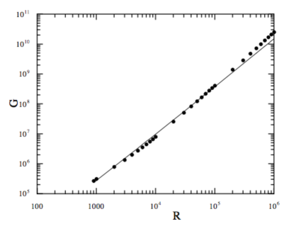
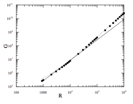
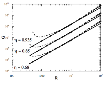
The second regime predicts torque varying more slowly than $R^{5/3}$. It could therefore only marginally explain the second regime observed by Wendt, for $R>10^{4}$, in which $G\sim R^{1.7}$. However, it could explain the regime obtained by LFS92 ; LewiSwin99 for $R\sim 10^{4}$, in which a continuously varying scaling exponent was obtained. This is shown in Fig. 3, where the fit to the data of LewiSwin99 is compared with the theoretical formula (21). The comparison is made using coefficients extrapolated from the small aspect ratio convection experiment: $K_{6}=20$, $K_{5}=2\pi K_{2}$ with $K_{2}=0.75\times 0.45$. It may happen however that this regime 2 does not exist in Taylor-Couette experiments. Indeed, since the temperature analog is related to the velocity, it might be impossible to excite velocity fluctuations without exciting pseudo-temperature fluctuations. This would mean a direct transition from regime 1 (mean flow dominated) to regime 3 (fluctuation dominated). This possibility is explored in Fig. 4, where we show the best fit of the measurements of Lewis and Swinney, with formula (22). This fit uses $K_{7}=0.50$ and $K_{8}=10^{4}$. Notice the big difference between these constants and their extrapolation from the convective case $K_{7}=0.145$ and $K_{8}=2\times 10^{7}$. This may reflect the sensitivity to boundary conditions of the regime 3. Note however that the fit is excellent from $R=10^{3}$ up to $R=10^{6}$. Below $R=10^{4}$, the regime 1 with $K_{2}=1.46$ fits the data very well also. As a last check, we have compared this regime 3 with the constant fitted for Lewis and Swinney’s data, to the data of Wendt. The result is shown in Fig. 5, for 3 different gap $\eta=0.68,0.85,0.935$. The agreement is excellent.

Figure 3: Torque vs Reynolds in Taylor-Couette experiments. The symbols are the data of LewiSwin99 . The line is the theoretical formula obtained in the hard turbulence regime and computed using the analogy with convection $G=AR^{5/3}/(\ln(R/B))^{2/3}$. The two constants $A$ and $B$ are not fitted to the data, but are analytically computed using the analogy with convection.

Figure 4: Torque vs Reynolds in Taylor-Couette experiments. The symbols are the data of LewiSwin99 . The lines are the theoretical formula obtained in the soft and ultra-hard turbulence regimes and computed using the analogy with convection. Soft turbulence eq. (20) (full line); ultra-hard turbulence eq. (22) (dotted line). In the former case, all the constants are analytically computed using the analogy. In the latter case, we have seek the best adjustment with data by adjusting the two constants.

Figure 5: Torque vs Reynolds in Taylor-Couette experiments for different gap widths $\eta=0.68$, $\eta=0.85$ and $\eta=0.935$. The symbols are the data of Wendt33 . The lines are the theoretical formula obtained in the soft and ultra-hard turbulence regimes and computed using the analogy with convection. Soft turbulence eq. (20) (full line); ultra-hard turbulence eq. (22) (dotted line). There is no adjustable parameter in this comparison, all the constants being fixed either by the analogy with convection, or by the comparison with the data of LewiSwin99 .

III.6 Velocity fluctuations

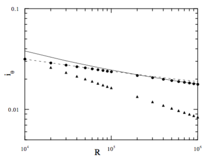
The analogy can also be used to predict the behavior of velocity fluctuations. In LewiSwin99 , the azimuthal turbulent intensity $i_{\theta}=\sqrt{<u_{\theta}^{2}>}/U_{\theta}$ was measured at midgap with hot film probes. Above $1\times 10^{4}$, a fit yields

$$i_{\theta}=0.10R^{-0.125}.$$ (23)

Using the analogy, this intensity is related to the temperature fluctuations at mid-gap, in the ultra hard turbulent regime (regime 3). The total analog temperature fluctuation in fact also includes vertical velocity fluctuations (see Table 1). In an axisymmetric turbulence, one could therefore expect that the turbulent intensity measured by Lewis and Swinney is proportional to the temperature analog. Recent measurements of this quantity at Rayleigh number up to $Ra=10^{15}$ have been measured by NSSD00 in a low aspect ratio Helium experiment. They found $\theta/\Delta T=0.37Ra^{-0.145}$, but this was obtained in a regime where the Nusselt number varies like in regime 2 (velocity fluctuation dominate but NOT temperature fluctuation). Using the analogy, this would translate into a regime where $i_{\theta}\sim R^{-0.29}$, in clear contradiction with the data of Lewis and Swinney, see Fig. 6. This might therefore be another proof of the absence of the regime 2 in Taylor-Couette experiment.

Unfortunately, we are not aware of temperature measurements in convective turbulence in the ultra-hard regime. In previous analysis of temperature fluctuations in the atmospheric boundary layer, Deardoff and Willis DearWill67 showed that temperature fluctuations follow the free convection regime

$$\frac{\theta}{\Delta T}\propto\frac{Nu}{(PrRaNu)^{1/3}},$$ (24)

where the proportionality constant is of the order 1. Fig. 6 shows the application of this scaling to the data of Lewis and Swinney, where the analogy was used to translate torque and Reynolds into Nusselt and Rayleigh. The best agreement with the experimental fit of Lewis and Swinney is obtained for a prefactor $1.8$. We can also compare the results with the theoretical prediction given by the convective model. In this model Dubr01 , the temperature fluctuations in the boundary layer obey:

$$\frac{<\theta^{\prime 2}>}{\Delta T^{2}}=\lambda_{u}\frac{Nu^{5/2}}{(RaPr)^{1/2}}\frac{\sqrt{1+(z/\lambda_{u})^{2}}}{1+(zNu)^{2}},$$ (25)

where $\lambda_{u}$ is the height of the viscous velocity layer. The value at the height of the boundary layer is obtained for $z=\lambda_{BL}$, the size of the boundary layer, which was shown to vary like $\lambda_{BL}\sim(RaNu)^{-1/8}/\sqrt{\ln(RaNu)}$. Assuming that the value at mid-gap equals this maximal value, we obtain:

$$\frac{\sqrt{<\theta^{\prime 2}>}}{\Delta T}=K_{10}\frac{Nu^{5/16}}{Ra^{3/16}}\left(\ln(RaNu/K_{11})\right)^{1/4}.$$ (26)

This prediction is shown in Fig. 6, using a fitted prefactors of $K_{10}=0.16$ and $K_{11}=1$. It is in very good agreement with the experimental fit of Lewis and Swinney.

Figure 6: Azimuthal velocity fluctuations in Taylor-Couette flow. The circles are the power-law fits of experimental measurements by LewiSwin99 . The triangles are the power-law fit to the temperature fluctuations (analog of azimuthal velocities) in Helium by NSSD00 . The line is the prediction obtained with the analog of the free-convective regime DearWill67 . The dotted line is the theoretical formula predicted by our model eq. (26).

IV Conclusion

In this paper, we have shown how a well-known analogy between stratified and rotating shear flows, for axi-symmetric perturbations, can be extended into the turbulent regime. Assuming predominance of the axi-symmetric perturbation in the turbulence dynamics , we used this analogy in the unstable case (analogy between convection and centrifugally unstable Taylor-Couette flow) to predict the scaling of the momentum transfer and velocity fluctuations. Our prediction is that at low Reynolds number, the non-dimensional torque follows (20) while at $R>10^{4}$, it follows (22). The analogy can also be used to discriminate between theories about Taylor-Couette turbulent quantities. For example, we have shown that the ”classical” $Nu\sim Ra^{1/3}$ regime, translate into a $G\sim Ra^{5/3}$ in the Taylor-Couette flow (both being unobserved experimentally at large Rayleigh or Reynolds number).

The analogy also sheds new light on the recent theory of Eckhardt et al EGL00 . It predicts a dependence: $G=c_{1}Re^{3/2+5\xi/2}+c_{2}Re^{2+3\xi}$, where $\xi=-0.051$ is a parameter which has been adjusted to a best fit. When translated using this analogy, this formula would give in the convective case: $Nu=c_{1}Ra^{1/4+5\xi/4}+c_{2}Ra^{1/2+3\xi/2}$. This has to be compared with the theoretical prediction of Grossman and Lohse GrosLohs00 , made using the same theory, which leads to $Nu=c_{1}Ra^{1/4}+c_{2}Ra^{1/3}$. Clearly, there is no value of $\xi$ which can reconciliate the two formulae. It would therefore be interesting to see whether the analog of the Grossman and Lohse formula, namely: $G=c_{1}=Re^{3/2}+c_{2}Re^{5/3}$ would not fit the data equally well than the Eckhardt et al formula. This would reduce the number of unknown parameter by one.

It would now be interesting to study in more details consequences of the analogy in the stable case (i.e. stably stratified flow v.s. centrifugally stable flow). There are many observational, numerical and experimental results in the case of stably stratified flows. However, their counter part in the centrifugally stable rotating case is presently missing. Recent experiments by Richard et al Richardthese performed on flows between counter-rotating cylinders could help filling this gap.

Finally, the analogy is of great interest for astrophysical and geophysical applications. In astrophysics, for example, many objects are differentially rotating, and are characterized by very large Reynolds number. These Reynolds numbers cannot be reached in laboratory experiments. On the other hand, we have at our disposal a natural high Rayleigh (and Reynolds number) laboratory of stratified turbulence: the atmospheric boundary layer. We believe that we could use all the data collected in our atmosphere to get great insight about large Reynolds number behavior of rotating, astrophysical shear flows, using the analogy sketched in the present paper.

We thank François Daviaud for comments on the manuscript.

stratified shear flow	rotating shear flow
$z$	$r$
$x$	$\theta$
$\partial_{z}U$	$r\partial_{r}\Omega$
$\beta g$	$2\frac{\Omega}{r}\sin^{2}\phi$
$\partial_{z}\Theta$	$\frac{1}{r}\partial_{r}(r^{2}\Omega)$
$w$	$u$
$\theta$	$(rv-w\cot\phi)$

Table 1: The detailed analogy between startified and rotating shear flow. The notations for the stratified case are from DLS02 .

References

- (1) C.R. Doering and P. Constantin Phys. Rev. Lett. 69 1648 (1992).
- (2) J.W. Deardoff and G.E Willis J. Fluid Mech. 28 675 (1967)
- (3) A. Esser and S. Grossmann Phys. Fluid 8 1814 (1996).
- (4) P. Bradshaw J. Fluid Mech. 36 177 (1969).
- (5) S. Chandrasekhar ” Hydrodynamic and hydromagnetic stability”, Clarendon (1970).
- (6) J.K. Platten and J.C. Legros ”Convection in liquids”, Springer-Verlag (1984).
- (7) A. Schlüter, D. Lortz and F. Busse J. Fluid Mech. 23 129 (1965).
- (8) D.P. Lathrop, J. Fineberg and H.L. Swinney Phys. Rev A 46, 6390 (1992).
- (9) R.L. Panton C.R. Acad. Sci, Ser. II, 315 1467 (1992).
- (10) D. Richard ”Instabilités hydrodynamiques dans les écoulements en rotation différentielle”, Thèse de l’Université Paris 7, 2001.
- (11) A. Barcilon and J. Brindley, J. Fluid Mech. 143 429 (1984).
- (12) G.P. King, Y. Li, W. Lee, H.L. swinney and P.S. Marcus J. Fluid Mech 41 365 (1984).
- (13) G.S. Lewis and H.L. Swinney Phys Rev. E 59 5457 (1999).
- (14) B. Castaing, G. Gunaratne, F. Heslot, L. Kadanoff, A. Libchaber,S. Thomae,X-Z. Wu, S. Zaleski and G. Zanetti J. Fluid Mech. 204 1 (1989).
- (15) R. Kraichnan Phys. Fluids 5 1374 (1962)
- (16) S. Grossmann and D. Lohse J. Fluid Mech. 407 27 (2000).
- (17) B. Echardt, S. Grossman and D. Lohse Eur. Phys. J B 18 541 (2000).
- (18) F. Wendt Ingenieur-Archiv. 4 577 (1933).
- (19) W.V.R. Malkus Proc. Roy. Soc. London., A 225, 185-195. (1954); W.V.R. Malkus Proc. Roy. Soc. London., A 225, 195-212. (1954)
- (20) J.J. Niemela, L. Skrbek, K.R. Sreenivasan and R.J. Donnelly Nature 404 837 (2000).
- (21) B. Dubrulle, J-P. Laval and P. Sullivan A dynamical subgrid scale model for the planetary surface layer II. to appear in J. Atmosph. Sci. (2002) preprint available at http://www.atmos.ucla.edu/ laval/PUBLI/publi.html
- (22) B. Dubrulle, Europhys. Letters 51 513 (2000).
- (23) B. Dubrulle, Euro. Phys. J. B 21 295 (2001).
- (24) B. Dubrulle, J-P. Laval, P. Sullivan and J. Werne A dynamical subgrid scale model for the planetary surface layer 1. The model to appear in J. Atmosph. Sci. (2002) preprint available at http://www.atmos.ucla.edu/ laval/PUBLI/publi.html .
- (25) S. Nazarenko, N. Kevlahan and B. Dubrulle Physica D 139 158 (2000).
- (26) B. Dubrulle, J-P. Laval, S. Nazarenko and N. Kevlahan to appear in Phys. Fluid (2001).
- (27) X. Chavanne, F. Chilla, B. Castaing, B. Hébral, B. Chabaud and J. Chaussy, Phys. Rev. Letters 79, 3648 (1997).
- (28) F. Heslot, B. Castaing and A. Libchaber Phys. Rev. A 36 5870 (1987).
- (29) W.V.R. Malkus and G. Veronis J. Fluid Mech. 4 225 (1958)
- (30) G.I. Taylor Proc. R. Soc. London A, 157 546 (1936).
- (31) P. Tong, W.I. Goldburg, J.S. Huang and T.A. Witten Phys. Rev. Lett. 65 2780 (1990).
- (32) J-P. Laval, B. Dubrulle and S. Nazarenko Non-locality and intermittency in 3D turbulence Phys. Fluids 13 1995-2012 (2001).