Gaussian Enveloped Decoherence of the Atomic States in Quantum Cavity

Abstract

We revisit the decoherence of the atomic state in the resonant Jaynes-Cummings model with the field initially being in a coherent state. We show that the purity of the atom exhibits oscillating Gaussian dependence on the time with a width independent of the initial atomic state. It is also shown that when the atom and the coherent state match each other in phase, the atomic decoherence is Gaussian time dependence.

1 Introduction

Quantum decoherence is at the heart of both the foundations and applications of quantum physics. Cavity quantum electrodynamics (QED) systems, operating in the strong coupling regime, have proven to be excellent for the studies of the entangled atom-photon state [1]. The experiment involving the Rydberg atoms in a high Q microwave cavity have opened the way to the studies of the decoherence dynamics in a mesoscopic system [2]. Theoretically, the simplest model that captures the physics of such a hybrid system is the Jaynes–Cummings (JC) model [3, 4]. It is one of the few exactly solvable models in quantum optics and predicts several interesting effects such as the vacuum field Rabi oscillations [5, 6, 7], collapses and revivals of Rabi oscillations in the coherent field [8]. Remarkably, it was noticed that the atom is to a good approximation in a pure state in the middle between the collapse and revival [9, 10].

On the other hand, being related to the quantum measurement theory and the quantum decoherence problems, the influence induced by the spin bath on the decoherence dynamics of a central system have also attracted much attention [11]. It was shown that the decoherence induced by coupling a system with an environment may display universal features: the decay of quantum coherences in the system is Gaussian for the specific initial environment state [12, 13, 14]

In this paper, we revisit the decoherence of the atomic state in the resonant JC model with the field initially being in a coherent state and elaborate the dynamic evolution of the purity. Closed analytical expressions for the purity of the central 2-level atoms are obtained. We observe that the similar behavior as that of the spin bath occurs in such a hybrid system. Both the first collapse and the amplitude of subsequent oscillation exhibit a Gaussian decay behavior.

The paper is organized as follows. In Sec. II, we introduce the main properties of JC model. In Sec. III, we evaluate the purity of the central 2-level atom. Section IV presents our summary and conclusion. In the Appendix we derive the main formula needed to evaluate various sums used in the text.

2 The JC model

Starting point of the analysis is the JC model, which consists of a single atom coupled to a single mode cavity. The two possible states of the atom are the ground state $\left|g\right\rangle$, and its excited state $\left|e\right\rangle$. The model and the subject we discussed are the same as the one previously studied by Gea–Banacloche [9, 10], who showed that the atom is to a good approximation in a pure state in the middle between the collapse time $t_{c}$ and revival time$\ t_{r}$. In the following, we will not only reproduce the results of [9, 10] but also show that this remarkable phenomenon is a part of the dynamical process for a special case. The model Hamiltonian at the resonance has the form

$$H = \lambda\left(\sigma_{+}a+\sigma_{-}a^{{\dagger}}\right)+\frac{1}{2}\omega_{a}\sigma_{z}+\omega a^{\dagger}a$$ (1)

$$\sigma_{+} = \left(\sigma_{-}\right)^{\dagger}=\left|e\right\rangle\left\langle g\right|,\sigma_{z}=\left|e\right\rangle\left\langle e\right|-\left|g\right\rangle\left\langle g\right|$$

where $a^{{\dagger}}$ is the creation operators of photon with frequency $\omega$, $\omega_{a}$ is the atomic transition frequency, and $\lambda$ is the cavity–atom coupling constant. The aim here is to study the dynamics of a given initial state. A general initial state of the system has the form

$$\left|\Psi\left(0\right)\right\rangle=\left(C_{g}\left|g\right\rangle+C_{e}\left|e\right\rangle\right){\sum_{n=0}^{\infty}}C_{n}\left|n\right\rangle$$ (2)

where $|C_{e}|^{2}+|C_{g}|^{2}=1$. Of central importance is the excitation number

$$\mathcal{N}=\frac{1}{2}\sigma_{z}+a^{\dagger}a+\frac{1}{2}$$ (3)

is a conserved quantity, i.e., $\left[\mathcal{N},H\right]=0$, which makes it easy to diagonalize the Hamiltonian, since the atom-field eigenspaces are only two-dimensional. It also makes the dynamics of states involving several subspaces simple. Nevertheless, the dynamics of states that have many significant energy-state components can show considerable complexity.

Introducing a unitary transformation

$$\mathcal{R}\left(\theta,\phi\right)=\mathrm{e}^{\mathrm{i}\left(\theta\sigma_{z}/2+\phi a^{\dagger}a\right)}$$ (4)

which generate the phases $\theta$ and $\phi$ on the atomic and cavity states

$$\mathcal{R}\left(\theta,\phi\right)\left(C_{g}\left|g\right\rangle+C_{e}\left|e\right\rangle\right)\left|n\right\rangle=\mathrm{e}^{\mathrm{i}n\phi}\left(\mathrm{e}^{-\mathrm{i}\theta/2}C_{g}\left|g\right\rangle+\mathrm{e}^{\mathrm{i}\theta/2}C_{e}\left|e\right\rangle\right)\left|n\right\rangle,$$ (5)

we have $\mathcal{R}H\mathcal{R}^{\dagger}=\tilde{H}$, where

$$\tilde{H} = \lambda\left(\sigma_{+}\tilde{a}+\sigma_{-}\tilde{a}^{{\dagger}}\right)+\frac{1}{2}\omega_{a}\sigma_{z}+\omega\tilde{a}^{{\dagger}}\tilde{a}$$

$$= \lambda\left(\tilde{\sigma}_{+}a+\tilde{\sigma}_{-}a^{{\dagger}}\right)+\frac{1}{2}\omega_{a}\tilde{\sigma}_{z}+\omega a^{\dagger}a$$

with $\tilde{a}=\mathrm{e}^{-\mathrm{i}\left(\phi-\theta\right)}a$, $\tilde{\sigma}_{+}=\mathrm{e}^{-\mathrm{i}\left(\phi-\theta\right)}\sigma_{+}$ and $\tilde{\sigma}_{z}=\sigma_{z}$. It indicates that Hamiltonians $H$ and $\tilde{H}$ share the same eigenfunctions by transformation of the basis $\left\{\left|n\right\rangle\right\}\rightarrow\left\{\mathrm{e}^{\mathrm{i}n\phi}\left|n\right\rangle\right\}$ or $\left|g\right\rangle\rightarrow\mathrm{e}^{-\mathrm{i}\theta/2}\left|g\right\rangle$ and $\left|e\right\rangle\rightarrow\mathrm{e}^{\mathrm{i}\theta/2}\left|e\right\rangle$. Remarkably, in the case of $\theta=\phi$, we have $\mathcal{R}H\mathcal{R}^{\dagger}=\tilde{H}=H$, which shows the invariance of the Hamiltonian under the transformation $\mathcal{R}\left(\theta,\theta\right)$. We will show that, when dealing with the coherent cavity state, this feature leads to an interesting and important phenomenon. We will demonstrate the strong dependence of the dynamics of the atomic purity on the relative phase of the atom and the cavity field.

We shall only consider the resonant case of $\omega=\omega_{a}$. Then at time $t$, state $\left|\Psi\left(0\right)\right\rangle$ evolves to

$$\left|\Psi\left(t\right)\right\rangle=\sum_{n=1}^{\infty}\left[C_{n}C_{g}\cos\left(\sqrt{n}\lambda t\right)-\mathrm{i}C_{n-1}C_{e}\sin\left(\sqrt{n}\lambda t\right)\right]\left|g,n\right\rangle$$ (7)

$$+\sum_{n=1}^{\infty}\left[C_{n}C_{e}\cos\left(\sqrt{n+1}\lambda t\right)-\mathrm{i}C_{n+1}C_{g}\sin\left(\sqrt{n+1}\lambda t\right)\right]\left|e,n\right\rangle],$$

We concern the reduced density matrix of the atom, which has the form

$$\rho_{A}\left(t\right)=\left(\begin{array}[]{cc}a&b\\ b^{\ast}&1-a\end{array}\right)$$ (8)

where

$$a = \sum_{n=1}^{\infty}\left[\left|C_{n}C_{g}\right|^{2}\cos^{2}\left(\sqrt{n}\lambda t\right)+\left|C_{n-1}C_{e}\right|^{2}\sin^{2}\left(\sqrt{n}\lambda t\right)\right.$$

$$\left.-2\mathrm{Im}\left(C_{n}C_{n-1}^{\ast}C_{g}C_{e}^{\ast}\right)\cos\left(\sqrt{n}\lambda t\right)\sin\left(\sqrt{n}\lambda t\right)\right],$$

$$b = \sum_{n=1}^{\infty}\left[\left|C_{n}\right|^{2}C_{g}C_{e}^{\ast}\cos\left(\sqrt{n}\lambda t\right)\cos\left(\sqrt{n+1}\lambda t\right)\right.$$

$$\left.+C_{n-1}C_{n+1}^{\ast}C_{e}C_{g}^{\ast}\sin\left(\sqrt{n}\lambda t\right)\sin\left(\sqrt{n+1}\lambda t\right)\right.$$

$$\left.+\mathrm{i}C_{n}C_{n+1}^{\ast}\left|C_{g}\right|^{2}\cos\left(\sqrt{n}\lambda t\right)\sin\left(\sqrt{n+1}\lambda t\right)\right.$$

$$\left.-\mathrm{i}C_{n-1}C_{n}^{\ast}\left|C_{e}\right|^{2}\sin\left(\sqrt{n}\lambda t\right)\cos\left(\sqrt{n+1}\lambda t\right)\right].$$

As a measure of the degree of coherence, the purity the atom can be expressed as

$$P(t)=\mathrm{Tr}\left(\rho_{A}^{2}\right)=a^{2}+\left(1-a\right)^{2}+2\left|b\right|^{2},$$ (10)

where Tr$\left(...\right)$ denotes the trace on the cavity field.

3 Decoherence of a two-level atom

With the time evolution of the reduced density matrix of the atom, we can investigate the dynamical behavior of the atom, which has been employed to calculate the inversion and the purity for the case of initial coherent state. The initial state has the form

$$\left|\Psi\left(0\right)\right\rangle=\left(C_{g}\left|g\right\rangle+C_{e}\left|e\right\rangle\right)\left|\alpha\right\rangle$$ (11)

where

$$\left|\alpha\right\rangle=\mathrm{e}^{-\left|\alpha\right|^{2}/2}\sum_{n=0}^{\infty}\frac{\alpha^{n}}{\sqrt{n!}}\left|n\right\rangle,\alpha=\mathrm{e}^{-\mathrm{i}\phi}\sqrt{{\bar{n}}}.$$ (12)

It is has been found that the initial Rabi-oscillations concerning the probability of being in a given atomic state decay on a timescale called the collapse time, $t_{c}=2/\lambda$, but then revive after a much longer time, $t_{r}=2\pi\sqrt{\bar{n}}/\lambda$ [15, 16].

Here we discuss the time dependence of the atomic purity in a long time scale. For $\left|\alpha\right|^{2}$ (or $\bar{n}$) $\gg 1$, we have

$$C_{n}=\mathrm{e}^{-\left|\alpha\right|^{2}/2}\frac{\alpha^{n}}{\sqrt{n!}}=\frac{\alpha}{\sqrt{n}}C_{n-1}\approx\mathrm{e}^{-\mathrm{i}\phi}C_{n-1}.$$ (13)

Remarks on flat condition. In the following we take $\phi=0$ for the sake of simplicity, since factor $\mathrm{e}^{-\mathrm{i}\phi}$ can be mapped on the atomic state by $\left(C_{g},C_{e}\right)\rightarrow\left(\mathrm{e}^{-\mathrm{i}\phi/2}C_{g}+\mathrm{e}^{\mathrm{i}\phi/2}C_{e}\right)$ according to our previous analysis. Then in the following derivation, we simply consider the coefficients $C_{g}$ and $C_{e}$ as complex numbers. On the other hand, for sufficiently large value of $\bar{n}$, the Poisson distribution is an approximation to the normal (or Gaussian) distribution, i.e.,

$$C_{n}C_{n-1}\approx C_{n}^{2}=\exp\left(-\bar{n}\right)\frac{\bar{n}^{n}}{n!}\approx\frac{1}{\sqrt{2\pi\bar{n}}}\exp\left[-\frac{\left(n-\bar{n}\right)^{2}}{2\bar{n}}\right].$$ (14)

On the other hand, the Poissonian function peaks sharply around $\bar{n}$. Then for a nontrivial function $F(\sqrt{n},1/\sqrt{n})$, one can take the approximation

$$C_{n}^{2}F(\sqrt{n},1/\sqrt{n})\approx\frac{1}{\sqrt{2\pi\bar{n}}}\exp\left[-\frac{\left(n-\bar{n}\right)^{2}}{2\bar{n}}\right]F(\frac{\sqrt{\bar{n}}}{2}+\frac{n}{2\sqrt{\bar{n}}},\frac{3}{2\sqrt{\bar{n}}}-\frac{n}{2\sqrt{\bar{n}^{3}}}).$$ (15)

Furthermore, in the limit of $\bar{n}\gg 1$ the summation over $n$ can be done exactly by virtue of Euler–Maclaurin formula. In the Appendix we derive the main formula needed to evaluate various sums used in the text. Accordingly, we obtain the analytic form for reduced density matrix elements are

$$a \approx \frac{1}{2}+\left[\frac{1}{2}\left(\left|C_{g}\right|^{2}-\left|C_{e}\right|^{2}\right)\cos\left(\frac{4\sqrt{\bar{n}}t}{t_{c}}\right)\right.$$

$$\left.+\left|C_{g}C_{e}\right|\sin\theta\sin\left(\frac{4\sqrt{\bar{n}}t}{t_{c}}\right)\right]\exp\left(-\frac{2t^{2}}{t_{c}^{2}}\right),$$

$$b \approx \left[\left|C_{g}C_{e}\right|\cos\theta\cos\left(\frac{\pi t}{t_{r}}\right)+\mathrm{i}\frac{1}{2}\sin\left(\frac{\pi t}{t_{r}}\right)\right]\exp\left(-\frac{\pi^{2}}{8\bar{n}}\frac{t^{2}}{t_{r}^{2}}\right)$$

$$+\mathrm{i}\left[\frac{1}{2}\left(\left|C_{g}\right|^{2}-\left|C_{e}\right|^{2}\right)\sin\left(\frac{4\sqrt{\bar{n}}t}{t_{c}}\right)\right.$$

$$\left.+\left|C_{g}C_{e}\right|\sin\theta\cos\left(\frac{4\sqrt{\bar{n}}t}{t_{c}}\right)\right]\exp\left(-\frac{2t^{2}}{t_{c}^{2}}\right)$$

From equation (10), we have

$$P(t) = \frac{1}{2}+2\left[\left|C_{g}C_{e}\right|^{2}\cos^{2}\theta\cos^{2}\left(\frac{\pi t}{t_{r}}\right)\right.\left.+\frac{1}{4}\sin^{2}\left(\frac{\pi t}{t_{r}}\right)\right]\exp\left(-\frac{\pi^{2}}{4\bar{n}}\frac{t^{2}}{t_{r}^{2}}\right)$$

$$+\frac{1}{2}\left[\left(\left|C_{g}\right|^{2}-\left|C_{e}\right|^{2}\right)^{2}+4\left|C_{g}C_{e}\right|^{2}\sin^{2}\theta\right]\exp\left(-\frac{4t^{2}}{t_{c}^{2}}\right)$$

$$+\sin\left(\frac{\pi t}{t_{r}}\right)\left[\left(\left|C_{g}\right|^{2}-\left|C_{e}\right|^{2}\right)\sin\left(\frac{4\sqrt{\bar{n}}t}{t_{c}}\right)\right.$$

$$\left.+2\left|C_{g}\right|\left|C_{e}\right|\sin\theta\cos\left(\frac{4\sqrt{\bar{n}}t}{t_{c}}\right)\right]\exp\left(-\frac{\pi^{2}}{8\bar{n}}\frac{t^{2}}{t_{r}^{2}}\right)\exp\left(-\frac{2t^{2}}{t_{c}^{2}}\right).$$

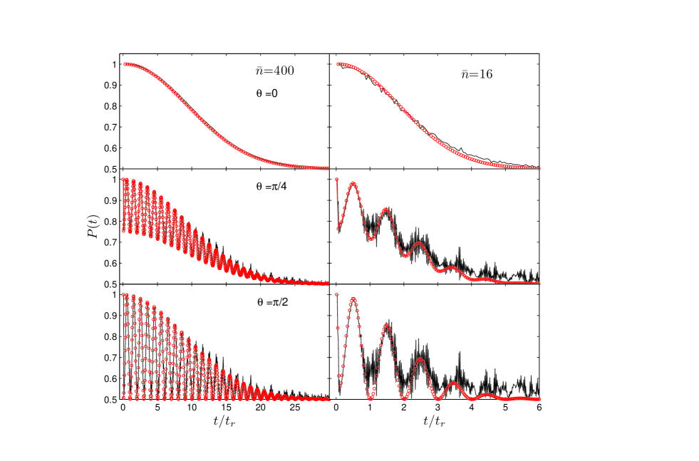
Figure 1: (Color online) Plots of the purity obtained by the exact diagonalization (solid line) and the approximate analytical expression equation (3) (empty circle) at various relative phases $\theta$, for the initial atomic state with $\left|C_{g}\right|=\left|C_{e}\right|$ and the initial coherent state of photons with average number $\bar{n}=400$ and $\bar{n}=16$.

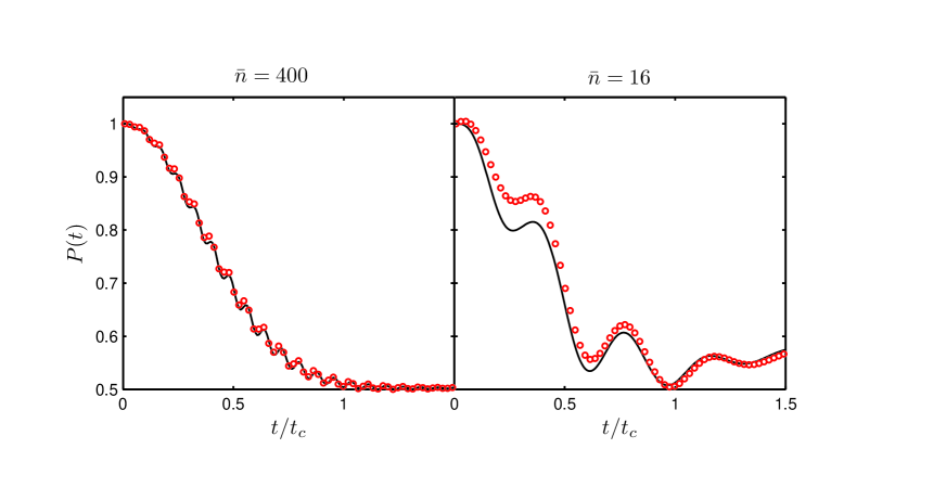
Figure 2: (Color online) The same as figure 1 but in the small time scale and the case of $\theta=\pi/2$.

We can see that, at small time region $t\ll t_{r}$, the term containing $\exp\left(-4t^{2}/t_{c}^{2}\right)$ is a transient state and is dominant at the beginning of the evolution. This Gaussian decay behavior is independent of the mean photon number $\bar{n}$. After the transient relaxation, the purity of the atom exhibits oscillating Gaussian dependence on the time. The width of Gaussian function is independent of the values of $C_{g}$ and $C_{e}$. The initial atomic state determines the amplitude of the oscillation. Both the first collapse and the amplitude of subsequent oscillation exhibit a Gaussian decay behavior. Using the analytic expressions for the purity amplitude equation (3), we estimate the period of the oscillation to be the same as that of the Rabi oscillation. Obviously, purity dynamics depends on the parameter of the system as well as the initial state. In this work we show that the relative phase between the initial atom and cavity field has far more important influence on the purity dynamics. Let us consider two interesting special cases: $\left|C_{g}C_{e}\right|=0$ and $\left|C_{g}\right|=\left|C_{e}\right|$. In first case, $C_{g}=0$ ( or $C_{e}=0$), we have

$$P_{\max}(t) = \frac{1}{2}+\frac{1}{2}\sin^{2}\left(\frac{\pi t}{t_{r}}\right)\exp\left(-\frac{\pi^{2}}{4\bar{n}}\frac{t^{2}}{t_{r}^{2}}\right)+\frac{1}{2}\exp\left(-\frac{4t^{2}}{t_{c}^{2}}\right)$$

$$\pm\sin\left(\frac{\pi t}{t_{r}}\right)\sin\left(\frac{4\sqrt{\bar{n}}t}{t_{c}}\right)\exp\left(-\frac{\pi^{2}}{8\bar{n}}\frac{t^{2}}{t_{r}^{2}}\right)\exp\left(-\frac{2t^{2}}{t_{c}^{2}}\right),$$

i.e., the amplitude of the oscillations becomes maximum. In second case, $C_{g}=\mathrm{e}^{\mathrm{i}\theta}C_{e}$, we have

$$P_{\theta}(t) = \frac{1}{2}+\frac{1}{2}\left[1-\sin^{2}\theta\cos^{2}\left(\frac{\pi t}{t_{r}}\right)\right]\exp\left(-\frac{\pi^{2}}{4\bar{n}}\frac{t^{2}}{t_{r}^{2}}\right)$$

$$+\frac{1}{2}\sin^{2}\theta\exp\left(-\frac{4t^{2}}{t_{c}^{2}}\right)$$

$$+\sin\left(\frac{\pi t}{t_{r}}\right)\sin\theta\cos\left(\frac{4\sqrt{\bar{n}}t}{t_{c}}\right)\exp\left(-\frac{\pi^{2}}{8\bar{n}}\frac{t^{2}}{t_{r}^{2}}\right)\exp\left(-\frac{2t^{2}}{t_{c}^{2}}\right).$$

It shows that after the transient process, the amplitude of the oscillations only depends on the relative phase $\theta$. We also note that $P_{\theta}(t)$ behaves as the purity for various values of the coefficients $C_{g}=\mathrm{e}^{-\mathrm{i}\delta/2}\left|C_{g}\right|$ and $C_{e}=\mathrm{e}^{\mathrm{i}\delta/2}\left|C_{e}\right|$ by simply replacing $\sin^{2}\theta$ in the equation (3)  with $1-4\left|C_{g}C_{e}\cos\delta\right|^{2}$. Thus in the following numerical simulations, we only demonstrate the case of $\left|C_{g}\right|=\left|C_{e}\right|$ for simplicity.

We note that in the case of $\theta=0$

$$P_{\min}(t)=\frac{1}{2}+\frac{1}{2}\exp\left(-\frac{\pi^{2}}{4\bar{n}}\frac{t^{2}}{t_{r}^{2}}\right),$$ (20)

which corresponds to the envelope of the pattern $P(t)$ for arbitrary initial atomic state.

The above analysis shows two important characteristics of the decoherence dynamics. At first, the decoherence occurs dramatically at the very beginning for an arbitrary initial atomic state except the case of $C_{g}=C_{e}$. Secondly, after the transient decoherence, the amplitude of the oscillating purity strongly depends on the initial phase difference between the atom and the field. When the initial atom and the field are in-phase or opposite-phase ($\phi-\theta=0$, $\pi$), the atom has a relatively long coherent time. When they are orthogonal-phase ($\phi-\theta=\pi/2$, $3\pi/2$), the atom acquires maximal oscillating amplitude of decoherence.

In order to verify the above analysis some numerical simulations are performed. In figure 1, we plot the equation (10) for $\bar{n}=400$ and $16$ cases with different values of $\theta$ and $\left|C_{g}\right|=\left|C_{e}\right|$. As comparison, we also plot the equation (3) accordingly. We can see that the analytical results match well with the simulation results, especially in large $\bar{n}$ case and during the first several periods of oscillation. figure 2 is the same as the plot in figure 1 but for small time scale and $\theta=\pi/2$ to demonstrate the transient process explicitly.

It is also worthwhile to mention that the Gaussian decay of the decoherence is the direct result of the coherent state environment. We note that the expression equation (3) is obtained under the two conditions: (i) distribution function $C_{n}$ is flat as equation (13); (ii) we can use the approximation equation (15) near the mean photon number $\bar{n}$. The result for $\theta=0$ may promise important potential applications in quantum-information processing since Gaussian time dependence of the decoherence factor would suggest a different more frequent error correction than the exponential dependence.

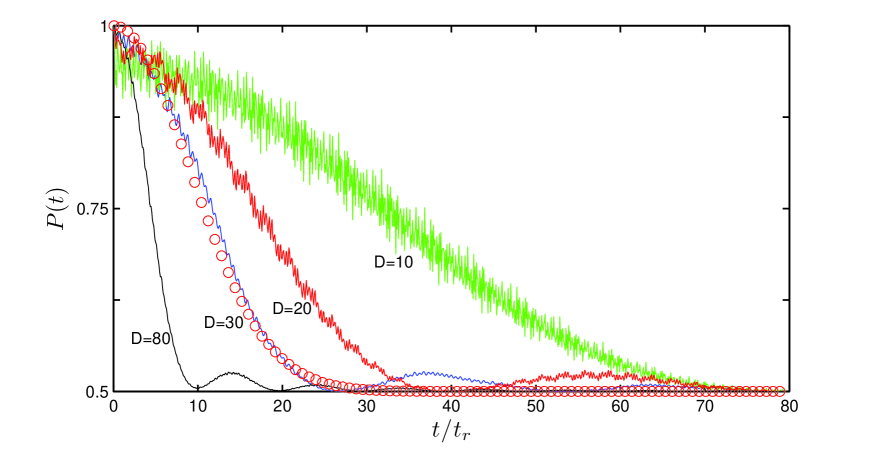
Figure 3: (Color online) Plots of the purity for the top-hat initial field states with average number $\bar{n}=400,$ $D=10$, $20$, $30$, and $80$, and the approximate analytical expression (empty circle) for the initial coherent state of the field with the same average number. It indicates that the atomic coherence decay differs from the Gaussian function except the special case.

4 Summary

In conclusion, considering a system consisting of a two-level atom, initially prepared in a coherent superposition of two levels, interacting with a coherent state of the field, we show that the dynamics of the atomic purity are sensitive to the relative phase between the atom and the cavity field. We also observe that the purity of the atom exhibits oscillating Gaussian dependence on the time with a width independent of the initial atomic state. Our results may have a great potential for future applications in quantum optical device.

References