A Subspace Estimator for Fixed Rank Perturbations
of Large Random Matrices

Abstract

This paper deals with the problem of parameter estimation based on certain eigenspaces of the empirical covariance matrix of an observed multidimensional time series, in the case where the time series dimension and the observation window grow to infinity at the same pace. In the area of large random matrix theory, recent contributions studied the behavior of the extreme eigenvalues of a random matrix and their associated eigenspaces when this matrix is subject to a fixed-rank perturbation. The present work is concerned with the situation where the parameters to be estimated determine the eigenspace structure of a certain fixed-rank perturbation of the empirical covariance matrix. An estimation algorithm in the spirit of the well-known MUSIC algorithm for parameter estimation is developed. It relies on an approach recently developed by Benaych-Georges and Nadakuditi [8, 9], relating the eigenspaces of extreme eigenvalues of the empirical covariance matrix with eigenspaces of the perturbation matrix. First and second order analyses of the new algorithm are performed.

1 Introduction

Parameter estimation algorithms based on the estimation of an eigenspace of the autocorrelation matrix of an observed multivariate time series are very popular in the areas of statistics and signal processing. Applications of such algorithms include the estimation of the angles of arrival of plane waves impinging on an array of antennas, the estimation of the frequencies of superimposed sine waves, or the resolution of multiple paths of a radio signal. Denoting by $N$ the signal dimension (e.g., the number of antennas) and by $n$ the length of the time observation window, the observed time series is represented by a $N\times n$ random matrix $\Sigma_{n}=X_{n}+P_{n}$ where $X_{n}$ and $P_{n}$ are respectively the so-called noise and signal matrices. In many applications, $P_{n}$ is represented as

$$P_{n}=B(\varphi_{1},\cdots\varphi_{r})S_{n}^{*}\ ,$$ (1)

where $(\varphi_{1},\ldots,\varphi_{r})$ are the $r\leq\min(N,n)$ deterministic parameters to be estimated, $B$ is a $N\times r$ matrix of the form $B(\varphi_{1},\cdots\varphi_{r})=\begin{bmatrix}b(\varphi_{1})&\cdots&b(\varphi_{r})\end{bmatrix}$ where $b(\varphi)$ is a known ${\mathbb{C}}^{N}$-valued function of $\varphi$, and the $S_{n}$ is an unknown $n\times r$ matrix with rank $r$ representing the signals transmitted by the $r$ emitting sources. As usual (and unless stated otherwise), $A^{*}$ stands for the Hermitian adjoint of matrix $A$. It will be assumed in this work that this matrix is deterministic. Often, the noise matrix $X_{n}$ is a complex random matrix such that the real and imaginary parts of its elements are $2Nn$ independent random variables with common probability law $\mathcal{N}(0,1/(2n))$. In this case, we shall say that $\sqrt{n}X_{n}$ is a standard Gaussian matrix.

We shall consider here “direction of arrival” vector functions $b(\varphi)$ that are typically met in the field of antenna processing. These functions are written

$$b(\varphi)=N^{-1/2}\begin{bmatrix}\exp(-\imath D\ell\varphi)\end{bmatrix}_{\ell=0}^{N-1}$$

with domain $\varphi\in[0,\pi/D]$ where $D$ is a positive real constant and $\imath^{2}=-1$. Assuming that the angular parameters $\varphi_{k}$ are all different, the well-known MUSIC (MUltiple SIgnal Classification, [27, 11]) algorithm for estimating these parameters from $\Sigma_{n}$ relies on the following simple idea: Assume that $\sqrt{n}X_{n}$ is standard Gaussian and let $\Pi$ be the orthogonal projection matrix on the eigenspace of ${\mathbb{E}}\Sigma_{n}\Sigma_{n}^{*}=BS_{n}^{*}S_{n}B^{*}+I_{N}$ associated with the $r$ largest eigenvalues, where $I_{N}$ is the $N\times N$ identity matrix. Obviously, $\Pi$ is the orthogonal projector on the column space of $B(\varphi_{1},\ldots,\varphi_{r})$. As a consequence, the angles $\varphi_{k}$ coincide with the zeros of the function $b(\varphi)^{*}(I-\Pi)b(\varphi)$ on $[0,\pi/D]$. Since $\|b(\varphi)\|=1$, they equivalently coincide with the maximum values (at one) of the so-called localization function $\chi(\varphi)=b(\varphi)^{*}\Pi b(\varphi)$.

In practice, $\Pi$ is classically replaced with the orthogonal projection matrix $\widehat{\Pi}$ on the eigenspace associated with the $r$ largest eigenvalues of $\Sigma_{n}\Sigma_{n}^{*}$. Assuming $N$ is fixed and $n\to\infty$, and assuming furthermore that $S_{n}^{*}S_{n}$ converges to some matrix $O>0$ in this asymptotic regime, the $\Sigma\Sigma^{*}\xrightarrow{\text{a.s.}}BOB^{*}+I_{N}$ by the Law of Large Numbers (a.s. stands for almost surely). Hence, the random variable $\chi_{\text{classical}}(\varphi)=b(\varphi)^{*}\widehat{\Pi}b(\varphi)$ a.s. converges to $\chi(\varphi)$, and it is standard to estimate the arrival angles as local maxima of $\chi_{\text{classical}}(\varphi)$.

However, in many practical situations, the signal dimension $N$ and the window length $n$ are of the same order of magnitude in which case the spectral norm of $\widehat{\Pi}-\Pi$ is not small, as we shall see below. In these situations, it is often more relevant to assume that both $N$ and $n$ converge to infinity at the same pace, while the number of parameters $r$ is kept fixed. The subject of this paper is to develop a new estimator better suited to this asymptotic regime, and to study its first and second order behavior with the help of large random matrix theory.

In large random matrix theory, much has been said about the spectral behavior of $X_{n}X_{n}^{*}$ in this asymptotic regime, for a wide range of statistical models for $X_{n}$. In particular, it is frequent that the spectral measure of this matrix converge to a compactly supported limiting probability measure $\pi$, and that the extreme eigenvalues of $X_{n}X_{n}^{*}$ a.s. converge to the edges of this support. Considering that $\Sigma_{n}$ is the sum of $X_{n}$ and a fixed-rank perturbation, it is well-known that $\Sigma_{n}\Sigma_{n}^{*}$ also has the limiting spectral measure $\pi$ [2, Lemma 2.2]. However, the largest eigenvalues of $\Sigma_{n}\Sigma_{n}^{*}$ have a special behavior: Under some conditions, these eigenvalues leave the support of $\pi$, and in this case, their related eigenspaces give valuable information on the eigenspaces of $P_{n}$. This paper shows how the angles $\varphi_{k}$ can be estimated from these eigenspaces.

The problem of the behavior of the extreme eigenvalues of large random matrices subjected to additive or multiplicative low rank perturbations (often called “spiked models”) have received a great deal of interest in the recent years. In this regard, the authors of [4, 5, 25] study the behavior of the extreme eigenvalues of a sample covariance matrix when the population covariance matrix has all but finitely many eigenvalues equal to one, a problem described in [20]. Reference [13] is devoted to the extreme eigenvalues of a Wigner matrix that incurs a fixed-rank additive perturbation. Fluctuations of these eigenvalues are studied in [4, 26, 25, 1, 13, 12, 6].

Recently, Benaych-Georges and Nadakuditi proposed in [8, 9] a powerful technique for characterizing the behavior of extreme eigenvalues and their associated eigenspaces for three generic spiked models: The models $X_{n}+P_{n}$ and $(I_{n}+P_{n})X_{n}$ when both $X_{n}$ and $P_{n}$ are Hermitian and $P_{n}$ is low-rank, and the model that encompasses ours $(X_{n}+P_{n})(X_{n}+P_{n})^{*}$ where $X_{n}$ and $P_{n}$ are rectangular. One feature of this approach is that it uncovers simple relations between the extreme eigenvalues and their associated eigenspaces on the one hand, and certain quadratic forms involving resolvents related with the non-perturbed matrix $X_{n}$ on the other. This makes the method particularly well-suited (but not limited to) the situation where $X_{n}$ is unitarily or bi-unitarily invariant, a situation that we shall consider in this paper. Indeed, in this situation, these quadratic forms exhibit a particularly simple behavior in the considered large dimensional asymptotic regime.

In this paper, we make use of the approach of [8, 9] to develop a new subspace estimator of the angles $\varphi_{k}$ based on the eigenspaces of the isolated eigenvalues of $\Sigma_{n}\Sigma_{n}^{*}$. We perform the first and second order analyses of this estimator that we call the “Spike MUSIC” estimator. Our mathematical developments differ somehow from those of [8, 9] and could have their own interest. They are based on two simple ingredients: The first is an analogue of the Poincaré-Nash inequality for the Haar distributed unitary matrices which has been recently discovered by Pastur and Vasilchuk [23], and the second is a contour integration method by means of which the first and second order analyses are done. The key step of the second order analysis of our estimator lies in the establishment of a Central Limit Theorem on the quadratic forms $b(\varphi_{i})^{*}\widehat{\Pi}_{i}b(\varphi_{i})$ where the $\widehat{\Pi}_{i}$ are the orthogonal projection matrices on certain eigenspaces of $\Sigma_{n}\Sigma_{n}^{*}$ associated with the isolated eigenvalues. The employed technique can easily be used to study the fluctuations of projections of other types of vectors on these eigenspaces.

We now state our general assumptions and introduce some notations.

Assumptions and Notations

We now state the general assumptions of the paper. Consider the sequence of $N\times n$ matrices $\Sigma_{n}=X_{n}+P_{n}$ where:

Assumption A1.

The dimensions $N,n$ satisfy: $N\leq n$, $n\to\infty$ and

$$\frac{N}{n}\to c\in(0,1]$$

(notation for this asymptotic regime: $n\to\infty$).

The following assumption on $X_{n}$ is widely used in the random matrix literature [18, 24]:

Assumption A2.

Matrices $X_{n}$ are random $N\times n$ bi-unitarily invariant matrices, i.e., each $X_{n}$ admits the singular value decomposition $X_{n}=L_{n}\Gamma_{n}R_{n}^{*}$ where $L_{n}$, the $N\times N$ matrix $\Gamma_{n}$ and $R_{n}$ are independent, $L_{n}$ is Haar distributed on the group ${\mathcal{U}}(N)$ of unitary $N\times N$ matrices, and $R_{n}$ is a $n\times N$ submatrix of a Haar distributed matrix on ${\mathcal{U}}(n)$.

We recall that the Stieltjes transform of a probability measure $\pi$ on the real line is the complex function

$$m(z)=\int\frac{1}{t-z}\pi(dt)\ ,$$

analytic on ${\mathbb{C}}_{+}=\{z:\Im(z)>0\}$.

Assumption A3.

Let $Q_{n}(z)=(X_{n}X_{n}^{*}-zI_{N})^{-1}$ be the resolvent associated with $X_{n}X_{n}^{*}$ and let $\alpha_{n}(z)=N^{-1}\operatorname*{tr}Q_{n}(z)$. For every $z\in{\mathbb{C}}_{+}$, $\alpha_{n}(z)$ a.s. converges to a deterministic function $m(z)$ which is the Stieltjes transform of a probability measure $\pi$ supported by the compact interval $[\lambda_{-},\lambda_{+}]$.

Assumption A4.

The quantity $\|X_{n}X_{n}^{*}\|$ a.s. converges to $\lambda_{+}$ as $n\to\infty$, where $\|\cdot\|$ denotes the spectral norm.

Let $\widetilde{Q}_{n}(z)=(X_{n}^{*}X_{n}-zI_{n})^{-1}$ and $\tilde{\alpha}_{n}(z)=n^{-1}\operatorname*{tr}\widetilde{Q}_{n}(z)$. Equivalently to the convergence assumed by Assumption A3, one may assume that $\tilde{\alpha}_{n}(z)$ a.s. converges on ${\mathbb{C}}_{+}$ to a deterministic function $\tilde{m}(z)$ which is the Stieltjes transform of a probability measure $\tilde{\pi}$. In that case, $\tilde{m}(z)=cm(z)-(1-c)/z$ and $\tilde{\pi}=c\pi+(1-c)\delta_{0}$.

Remark 1.

In the areas of signal processing and communication theory, the noise matrix $X_{n}$ satisfying Assumptions A2-A4 is such that $\sqrt{n}X_{n}$ is standard Gaussian - see for instance [21], [15].

We first make a general assumption on matrices $P_{n}$; it will be specified later, and adapted to the context of the MUSIC algorithm:

Assumption A5.

Matrices $P_{n}$ are deterministic with a fixed rank equal to $r$ for all $n$ large enough. Denoting by $P_{n}=U_{n}\Omega_{n}V_{n}^{*}$ a singular value decomposition of $P_{n}$, the matrix of singular values $\Omega_{n}=\operatorname*{diag}(\omega_{1,n},\ldots,\omega_{r,n})$ with $\omega_{1,n}\geq\omega_{2,n}\geq\cdots\geq\omega_{r,n}$ converges to

$$O=\begin{bmatrix}\omega_{1}I_{j_{1}}&&\\ &\ddots&\\ &&\omega_{s}I_{j_{s}}\end{bmatrix}\ ,$$ (2)

where $\omega_{1}>\cdots>\omega_{s}>0$ and $j_{1}+\cdots+j_{s}=r$.

Notations.

As usual, if $z\in\mathbb{C}$, we shall denote by $\Re(z)$ and $\Im(z)$ its real and imaginary parts. We shall denote by $\xrightarrow[]{a.s.}$ (resp. $\xrightarrow[]{\mathcal{P}}$, $\xrightarrow[]{\mathcal{D}}$) the almost sure convergence (resp. convergence in probability, in distribution). We denote by $\delta_{i,j}$ the Kronecker delta ($=1$ if $i=j$ and $0$ otherwise).

The eigenvalues of $\Sigma_{n}\Sigma_{n}^{*}$ are $\hat{\lambda}_{1,n}\geq\hat{\lambda}_{2,n}\geq\cdots\geq\hat{\lambda}_{N,n}$. Associated eigenvectors will be denoted $\hat{u}_{1,n},\hat{u}_{2,n},\cdots,\hat{u}_{N,n}$. For $k\in\{1,\ldots,r\}$, we shall denote by $i(k)$ the index $i\in\{1,\ldots,s\}$ such that $j_{1}+\cdots+j_{i-1}<k\leq j_{1}+\cdots+j_{i}$. For $i=1,\ldots,s$, We shall denote by $\widehat{\Pi}_{i,n}$ the orthogonal projection matrix on the eigenspace of $\Sigma_{n}\Sigma_{n}^{*}$ associated with the eigenvalues $\hat{\lambda}_{k,n}$ such that $i(k)=i$, i.e., $\widehat{\Pi}_{i,n}=\sum_{k:i(k)=i}\hat{u}_{k,n}\hat{u}_{k,n}^{*}$ when this eigenspace is defined. Columns of $U_{n}$ (see A5) will be denoted $u_{1,n},\cdots,u_{r,n}$. Given $i$, the orthogonal projection matrix on the eigenspace of $P_{n}P_{n}^{*}$ associated with the eigenvalues $\omega_{k,n}^{2}$ such that $i(k)=i$ will be $\Pi_{i,n}=\sum_{k:i(k)=i}u_{k,n}u_{k,n}^{*}$. Indexes $n$ and $N$ will often be dropped for readability.

Paper organization

The paper is organized as follows. Section 2 is devoted to the mathematical preliminaries. The general approach is described in Section 3. The Spike MUSIC algorithm is presented in Section 4 along with a first order study of this algorithm. Fluctuations of the estimates of the $\varphi_{k}$ are studied in Section 5 under the form of a Central Limit Theorem.

2 Preliminary mathematical results

We shall need the two following results. The first one is well-known [23]. The second result, due to Pastur and Vasilchuk, is the unitary analogue of the well-known Poincaré-Nash inequality.

Lemma 1.

Let $W=[w_{ij}]$ be a random matrix Haar distributed on ${\mathcal{U}}(n)$. Then

$${\mathbb{E}}\left[w_{ij}w^{*}_{i^{\prime}j^{\prime}}\right]=\frac{1}{n}\delta_{i,i^{\prime}}\delta_{j,j^{\prime}}\ .$$

Lemma 2 ([23, 24]).

Let $\Phi:{\mathcal{U}}(n)\to{\mathbb{C}}$ be a function that admits a $C^{1}$ continuation to an open neighborhood of ${\mathcal{U}}(n)$ in the whole algebra of $n\times n$ complex matrices. Then

$$\operatorname*{var}\Phi(W_{n})={\mathbb{E}}\left|\Phi(W_{n})\right|^{2}-\left|{\mathbb{E}}\Phi(W_{n})\right|^{2}\leq\frac{1}{n}\sum_{j,k=1}^{n}{\mathbb{E}}\left|\Phi^{\prime}(W_{n})\cdot\left({\bf e}_{j}{\bf e}_{k}^{\mathrm{T}}W_{n}\right)\right|^{2}$$

where ${\mathbb{E}}$ is the expectation with respect to the Haar measure on ${\mathcal{U}}(n)$, where $\Phi^{\prime}$ is the differential of $\Phi$ as a function on ${\mathbb{R}}^{2n^{2}}$ acting on the matrix ${\bf e}_{j}{\bf e}_{k}^{\mathrm{T}}W_{n}$ seen as an element of ${\mathbb{R}}^{2n^{2}}$, and where ${\bf e}_{j}=[0\cdots 0\,1\,0\cdots 0]^{*}$ is the $j^{\text{th}}$ canonical vector of ${\mathbb{C}}^{n}$.

Given a small $\varepsilon_{1}>0$, let $O_{n}$ be the probability event

$$O_{n}=\left\{\|X_{n}X_{n}^{*}\|\leq\lambda_{+}+\varepsilon_{1}\right\}\ .$$ (3)

By Assumption A4, ${\mathbbm{1}}_{O_{n}}\xrightarrow{\text{a.s.}}1$ as $n\to\infty$.

Lemma 3.

Let Assumption A2 holds true and let $u,v$ be two unit norm deterministic $N\times 1$ vectors such that $u^{*}v=0$. Then for any $z$ with $\Re(z)>\lambda_{+}+\varepsilon_{1}$,

$${\mathbb{E}}\left|{\mathbbm{1}}_{O_{n}}\times u^{*}\left(Q(z)-\alpha(z)I\right)u\right|^{p} \leq \frac{K_{p}}{N^{p/2}d(z,\lambda_{+}+\varepsilon_{1})^{p}}\ ,$$

$${\mathbb{E}}\left|{\mathbbm{1}}_{O_{n}}\times u^{*}Q(z)v\right|^{p} \leq \frac{K_{p}}{N^{p/2}d(z,\lambda_{+}+\varepsilon_{1})^{p}}\ ,$$

where the constant $K_{p}$ only depends on $p$, and where $d(z,z^{\prime})$ is the Euclidean distance between $z$ and $z^{\prime}$ in $\mathbb{C}$.

Proof.

Recall that $X=L\,\Gamma\,R^{*}$ by Assumption A2; let $D=(\Gamma^{2}-zI)^{-1}$; write:

$$\begin{bmatrix}&u^{*}&\\ &v^{*}&\end{bmatrix}\left(Q-\alpha I\right)\begin{bmatrix}\\ u&v\\ \\ \end{bmatrix}=\begin{bmatrix}&w_{1}^{*}&\\ &w_{2}^{*}&\end{bmatrix}\left(D-\frac{\operatorname*{tr}D}{N}I\right)\begin{bmatrix}\\ w_{1}&w_{2}\\ \\ \end{bmatrix}.$$

Thanks to A2, $w_{1}$ and $w_{2}$ are the first two columns of a $N\times N$ unitary Haar distributed matrix $W=[w_{ij}]$ independent of $D$. Let $M={\mathbbm{1}}_{O_{n}}\times\left(D-N^{-1}(\operatorname*{tr}D)I\right)$ and $\Phi_{i}(W)=w_{1}^{*}Mw_{i}$ for $i=1,2$. Then ${\mathbb{E}}\Phi_{1}(W)={\mathbb{E}}\Phi_{2}(W)=0$ by Lemma 1. Applying Lemma 2 to $\Phi_{i}$ after noticing that $\Phi_{i}^{\prime}(W)\cdot A={\bf e}_{1}^{\mathrm{T}}A^{*}Mw_{i}+w_{1}^{*}MA{\bf e}_{i}$ for any $N\times N$ matrix $A$, we obtain:

$${\mathbb{E}}|\Phi_{i}|^{2}=\operatorname*{var}(\Phi_{i}) \leq\frac{1}{N}\sum_{j,k=1}^{N}{\mathbb{E}}\left|w_{k1}^{*}[MW]_{ji}+[W^{*}M]_{1j}w_{ki}\right|^{2}\ ,$$

$$\leq\frac{2}{N}{\mathbb{E}}\left(\|Mw_{i}\|^{2}+\|Mw_{1}\|^{2}\right)\ ,$$

$$\leq\frac{8}{Nd(z,\lambda_{+}+\varepsilon_{1})^{2}}\ .$$

We now proceed by induction; assume that the result is true until $p\geq 1$. Applying Lemma 2 to $\Phi_{i}^{(p+1)/2}$, we obtain:

$$\operatorname*{var}\Bigl{(}\Phi_{i}^{\frac{p+1}{2}}\Bigr{)} \leq\frac{1}{N}\sum_{j,k=1}^{N}{\mathbb{E}}\left|\frac{p+1}{2}\Phi_{i}^{\frac{p-1}{2}}\Phi^{\prime}_{i}(W)\cdot\left({\bf e}_{j}{\bf e}_{k}^{\mathrm{T}}W\right)\right|^{2}\ ,$$

$$\leq\frac{(p+1)^{2}}{2N}{\mathbb{E}}\left(\left|\Phi_{i}\right|^{p-1}\left(\|Mw_{i}\|^{2}+\|Mw_{1}\|^{2}\right)\right)\ ,$$

$$\leq\frac{2(p+1)^{2}K_{p-1}}{d(z,\lambda_{+}+\varepsilon_{1})^{p+1}N^{(p+1)/2}}\ .$$

Using again the induction hypothesis, we get:

$${\mathbb{E}}\left|\Phi_{i}\right|^{p+1}=\operatorname*{var}\Bigl{(}\Phi_{i}^{\frac{p+1}{2}}\Bigr{)}+\left|{\mathbb{E}}\Phi_{i}^{\frac{p+1}{2}}\right|^{2}\\ \leq\frac{2(p+1)^{2}K_{p-1}+K_{(p+1)/2}^{2}}{d(z,\lambda_{+}+\varepsilon_{1})^{p+1}N^{(p+1)/2}}=\frac{K_{p+1}}{d(z,\lambda_{+}+\varepsilon_{1})^{p+1}N^{(p+1)/2}}\ ,$$

which concludes the proof. ∎

Lemma 4.

Let Assumption A2 hold true; let $u,v$ be two unit norm deterministic vectors with respective dimensions $N\times 1$ and $n\times 1$. Then for any $z$ such as $\Re(z)>\lambda_{+}+\varepsilon_{1}$,

$${\mathbb{E}}\left|{\mathbbm{1}}_{O_{n}}\times u^{*}X\widetilde{Q}(z)v\right|^{p}\leq\frac{K_{p}}{n^{p/2}d(z,\lambda_{+}+\varepsilon_{1})^{p}}.$$

Proof.

Let $C=\Gamma(\Gamma^{2}-zI)^{-1}$. By Assumption A2, $u^{*}X\widetilde{Q}(z)v=w^{*}C\tilde{w}=\Phi(w)$ where $w$ is a vector uniformly distributed on the unit sphere of ${\mathbb{C}}^{N}$, $\tilde{w}$ is a vector uniformly distributed on the unit sphere of ${\mathbb{C}}^{n}$ and truncated to its first $N$ elements, and $w$, $\tilde{w}$ and $C$ are independent. The lemma is proved as above by applying Lemma 2 to $\Phi$ and by taking the expectation with respect to the law of $w$. ∎

Lemma 5.

Let Assumptions A1-A4 hold true. Let ${\mathcal{C}}$ be a closed path of ${\mathbb{C}}$ such that $\min_{z\in{\mathcal{C}}}\Re(z)>\lambda_{+}$. Fix the integer $r\leq N$ and let $U_{n}$ and $V_{n}$ be two deterministic isometry matrices with dimensions $N\times r$ and $n\times r$ respectively. Then

$$\sup_{z\in{\mathcal{C}}}\|U_{n}^{*}\left(Q_{n}(z)-m(z)I_{N}\right)U_{n}\| \xrightarrow[n\to\infty]{\text{a.s.}} 0\ ,$$

$$\sup_{z\in{\mathcal{C}}}\|V_{n}^{*}\left(\widetilde{Q}_{n}(z)-\tilde{m}(z)I_{n}\right)V_{n}\| \xrightarrow[n\to\infty]{\text{a.s.}} 0\ ,$$

$$\sup_{z\in{\mathcal{C}}}\|U_{n}^{*}X_{n}\widetilde{Q}_{n}(z)V_{n}\| \xrightarrow[n\to\infty]{\text{a.s.}} 0\ .$$

Proof.

Recall the definition (3) of the set $O_{n}$ and assume that $\varepsilon_{1}$ is chosen such that $\min_{z\in{\mathcal{C}}}\Re(z)>\lambda_{+}+\varepsilon_{1}$; let

$$h_{n}(z)={\mathbbm{1}}_{O_{n}}\times U_{n}^{*}\left(Q_{n}(z)-\alpha_{n}(z)I_{N}\right)U_{n}\ .$$

For any $\ell,s\leq r$, $[h_{n}]_{\ell,s}$ is a holomorphic function on ${\mathbb{C}}-[0,\lambda_{+}+\varepsilon_{1}]$. Consider a denumerable sequence of points $(z_{k})$ in ${\mathbb{C}}-[0,\lambda_{+}+\varepsilon_{1}]$ with an accumulation point in that set. By Lemma 3 with $p=3$, Markov inequality and Borel-Cantelli’s lemma, there exists a probability one set on which $[h_{n}(z_{k})]_{\ell,s}\to 0$ for every $k$. Moreover, the $\left|[h_{n}(z_{k})]_{\ell,s}\right|$ are uniformly bounded on any compact set of ${\mathbb{C}}-[0,\lambda_{+}+\varepsilon_{1}]$. By the normal family theorem, every $n$-sequence of $[h_{n}]_{\ell,s}$ contains a further subsequence which converges uniformly on the compact set ${\mathcal{C}}\subset{\mathbb{C}}-[0,\lambda_{+}+\varepsilon_{1}]$ to a holomorphic function that we denote $h^{*}$. Since $h^{*}(z_{k})=0$ for all $k$, $h^{*}(z)=0$ on ${\mathcal{C}}$, hence $\left|[h_{n}(z)]_{\ell,s}\right|$ converges uniformly to zero on ${\mathcal{C}}$ with probability one, and thanks to Assumption A4, $\|U^{*}\left(Q(z)-\alpha(z)I\right)U\|\to 0$ uniformly on ${\mathcal{C}}$ with probability one. The same argument, used in conjunction with Assumption A3, shows that with probability one, $\alpha(z)-m(z)\to 0$ uniformly on ${\mathcal{C}}$, and the first assertion is proven. The second and third assertions are proven similarly, the third being obtained with the help of Lemma 4. ∎

3 Fixed Rank Perturbations: First Order Behavior

We first recall a result on matrix analysis that can be found in [19, Th. 7.3.7]:

Lemma 6.

Given a $N\times n$ matrix $A$ with $N\leq n$, let ${\bf A}$ be the matrix:

$${\bf A}=\begin{bmatrix}0&A\\ A^{*}&0\end{bmatrix}.$$

Then $\sigma_{1},\cdots,\sigma_{N}$ are the singular values of $A$ if and only if $\sigma_{1},\cdots,\sigma_{N},-\sigma_{1},\cdots,-\sigma_{N}$ in addition to $n-N$ zeros are the eigenvalues of ${\bf A}$. Furthermore, a pair $(u,v)$ of unit norm vectors is a pair of (left,right) singular vectors of $A$ associated with the singular value $\sigma$ if and only if $\begin{bmatrix}u/\sqrt{2}\\ v/\sqrt{2}\end{bmatrix}$ is a unit norm eigenvector of ${\bf A}$ associated with the eigenvalue $\sigma$.

Along the ideas in [8, 9], we now characterize the behavior of the largest eigenvalues of $\Sigma\Sigma^{*}$, and then focus on their eigenspaces.

Asymptotic behavior of the largest eigenvalues of $\Sigma\Sigma^{*}$

We start with an informal description of the approach. By Lemma 6, $\lambda$ is an eigenvalue of $\Sigma\Sigma^{*}$ if and only if $\det(\boldsymbol{\Sigma}-\sqrt{\lambda}I)=0$ where ${\boldsymbol{\Sigma}}=\begin{bmatrix}0&\Sigma\\ \Sigma^{*}&0\end{bmatrix}$. Writing:

$${\boldsymbol{\Sigma}}=\begin{bmatrix}0&X\\ X^{*}&0\end{bmatrix}+\begin{bmatrix}U&0\\ 0&V\Omega\end{bmatrix}\begin{bmatrix}0&I_{r}\\ I_{r}&0\end{bmatrix}\begin{bmatrix}U^{*}&0\\ 0&\Omega V^{*}\end{bmatrix}\stackrel{{\scriptstyle\triangle}}{{=}}{\bf X}+BJB^{*}\ ,$$ (4)

and assuming that $x>0$ is not a singular value of $X$, we have:

$$\det(\boldsymbol{\Sigma}-{x}I)=\det({\bf X}-{x}I+BJB^{*})=\det(J)\det({\bf X}-{x}I)\det(J+B^{*}({\bf X}-{x}I)^{-1}B)\ ,$$

after noticing that $J=J^{-1}$. Using the formula for the inversion of a partitioned matrix (see [19])

$$\begin{bmatrix}A_{11}&A_{12}\\ A_{12}^{*}&A_{22}\end{bmatrix}^{-1}=\begin{bmatrix}(A_{11}-A_{12}A_{22}^{-1}A_{12}^{*})^{-1}&-A_{11}^{-1}A_{12}(A_{22}-A_{12}^{*}A_{11}^{-1}A_{12})^{-1}\\ -(A_{22}-A_{12}^{*}A_{11}^{-1}A_{12})^{-1}A_{12}^{*}A_{11}^{-1}&(A_{22}-A_{12}^{*}A_{11}^{-1}A_{12})^{-1}\end{bmatrix}\ ,$$

we obtain:

$${\bf Q}({x})=({\bf X}-{x}I)^{-1}=\begin{bmatrix}-{x}I&X\\ X^{*}&-{x}I\end{bmatrix}^{-1}=\begin{bmatrix}{x}Q(x^{2})&X\widetilde{Q}(x^{2})\\ \widetilde{Q}(x^{2})X^{*}&{x}\widetilde{Q}(x^{2})\end{bmatrix}\ .$$ (5)

Therefore,

$$\det(\boldsymbol{\Sigma}-{x}I)=\det(J)\det({\bf X}-{x}I)\det\widehat{H}(x)\ ,$$

where

$$\widehat{H}_{n}(x)=\begin{bmatrix}{x}U^{*}Q(x^{2})U&I_{r}+U^{*}X\widetilde{Q}(x^{2})V\Omega\\ I_{r}+\Omega V^{*}\widetilde{Q}(x^{2})X^{*}U&{x}\Omega V^{*}\widetilde{Q}(x^{2})V\Omega\end{bmatrix}$$

whence for $n$ large enough, the isolated eigenvalues of $\Sigma\Sigma^{*}$ above $\lambda_{+}$ will coincide with the zeros of $\det\widehat{H}(\sqrt{x})$ that lie above $\lambda_{+}$. Under Assumptions A1-A5, Lemma 5 shows that $\widehat{H}(x)$ a.s. converges to

$$H(x)=\begin{bmatrix}{x}m(x^{2})I_{r}&I_{r}\\ I_{r}&{x}\tilde{m}(x^{2})O^{2}\end{bmatrix}.$$

Consider the equation

$$\det H(\sqrt{x})=\det\left(xm(x)\tilde{m}(x)O^{2}-I_{r}\right)=0\ ,$$

and notice that the function

$$g(x)=xm(x)\tilde{m}(x)=x\left(\int\frac{1}{t-x}\pi(dt)\right)\left(c\int\frac{1}{t-x}\pi(dt)-\frac{1-c}{x}\right)$$ (6)

decreases from $g(\lambda_{+}^{+})=\lim_{x\downarrow\lambda_{+}}g(x)$ to zero on $(\lambda_{+},\infty)$. Let $\omega_{1}^{2}>\cdots>\omega_{q}^{2}$ be those among the diagonal elements of $O^{2}$ that satisfy $\omega_{i}^{2}>1/g(\lambda_{+}^{+})$. Equation $g(x)=\omega_{i}^{-2}$ will have a unique solution $x=\rho_{i}>\lambda_{+}$ for any $i=1,\cdots,q$, while it will have no solution larger than $\lambda_{+}$ for $i>q$. It is then expected that any eigenvalue $\hat{\lambda}_{k,n}$ of $\Sigma_{n}\Sigma_{n}^{*}$ for which $i(k)\leq q$ (remember the definition of $i(k)$ provided in the paragraph “Assumptions and Notations” in Section 1), will converge to $\rho_{i}$, while $\hat{\lambda}_{j_{1}+\cdots+j_{q}+1,n}\to\lambda_{+}$ almost surely.

These facts are formalized in the following theorem, shown in [7, 9]:

Theorem 1.

Let Assumptions A1-A5 hold true; let $q$ be the maximum index such that $\omega_{q}^{2}>1/g(\lambda_{+}^{+})$. Let $\rho_{i}$ be the unique real number $>\lambda_{+}$ satisfying $\omega_{i}^{2}g(\rho_{i})=1$ for $i=1,\cdots,q$. Then

$$\hat{\lambda}_{j_{1}+\cdots+j_{i-1}+\ell,n}\xrightarrow[n\to\infty]{\text{a.s.}}\rho_{i}$$

for $i=1,\cdots,q$ and $\ell=1,\cdots,j_{i}$ while

$$\hat{\lambda}_{j_{1}+\cdots+j_{q}+1,n}\xrightarrow[n\to\infty]{\text{a.s.}}\lambda_{+}\ .$$

In the case where $\sqrt{n}X$ is a standard Gaussian matrix, $\pi$ is the Marčenko-Pastur distribution with support $\operatorname*{supp}(\pi)=[\lambda_{-},\lambda_{+}]=[(1-\sqrt{c})^{2},(1+\sqrt{c})^{2}]$, and

$$m(x)=\frac{1}{2cx}\left(1-c-x+\sqrt{(1-c-x)^{2}-4cx}\right)$$ (7)

for $x\in(\lambda_{+},\infty)$. After a few derivations, we obtain:

Corollary 1.

Assume $\sqrt{n}X$ is standard Gaussian. Let $q$ be the maximum index such that $\omega_{q}^{2}>\sqrt{c}$. Then

$$\hat{\lambda}_{j_{1}+\cdots+j_{i-1}+\ell,n}\xrightarrow[n\to\infty]{\text{a.s.}}\frac{(\omega_{i}^{2}+1)(\omega_{i}^{2}+c)}{\omega_{i}^{2}}\quad\text{for}\ i=1,\ldots,q\ ,$$

and $\hat{\lambda}_{j_{1}+\cdots+j_{q}+1,n}\xrightarrow[n\to\infty]{\text{a.s.}}(1+\sqrt{c})^{2}$.

We now turn our attention to the eigenspaces of the isolated eigenvalues.

Asymptotic behavior of certain bilinear forms.

Recall the definition of $s$ as provided in Assumption A5. Given $i\leq s$, assume that $\omega_{i}^{2}>1/g(\lambda_{+}^{+})$. Given two $N\times 1$ deterministic sequences of vectors $b_{1,n}$ and $b_{2,n}$ with bounded norms, we shall find here a simple asymptotic relation between $b_{1,n}^{*}\widehat{\Pi}_{i,n}b_{2,n}$ and $b_{1,n}^{*}\Pi_{i,n}b_{2,n}$, that will be at the basis of the Spike MUSIC algorithm. A close problem has been considered in [9]. We consider here a different technique, based on a contour integration and on the use of Lemmas 3 and 4. This method lends itself easily to the first and second order analyses of the Spike MUSIC algorithm that we shall develop in the following sections.

Writing ${\bf b}_{i}=\begin{bmatrix}b_{i}\\ 0\end{bmatrix}$ with $i=1,2$, we have by virtue of Lemma 6:

$$b_{1}^{*}\widehat{\Pi}_{i}b_{2}=\frac{-1}{\imath\pi}\oint_{{\mathcal{C}}_{i,n}}{\bf b}_{1}^{*}\left({\boldsymbol{\Sigma}}-zI\right)^{-1}{\bf b}_{2}\ dz\ ,$$

where ${\mathcal{C}}_{i,n}$ is a positively oriented circle that encloses the only singular values $\sqrt{\hat{\lambda}_{k,n}}$ of $\Sigma_{n}$ for which $i(k)=i$. Recalling (4) and using Woodbury’s identity ([19, §0.7.4]) together with the fact that $J=J^{-1}$, we obtain:

$$b_{1}^{*}\widehat{\Pi}_{i}b_{2}=\frac{-1}{\imath\pi}\oint_{{\mathcal{C}}_{i}}{\bf b}_{1}^{*}{\bf Q}(z){\bf b}_{2}\ dz\\ +\frac{1}{\imath\pi}\oint_{{\mathcal{C}}_{i}}{\bf b}_{1}^{*}{\bf Q}(z)B\left(J+B^{*}{\bf Q}(z)B\right)^{-1}B^{*}{\bf Q}(z){\bf b}_{2}\ dz\ .$$ (8)

Using (5), we obtain after a straightforward calculation:

$$b_{1,n}^{*}\widehat{\Pi}_{i,n}b_{2,n}=\frac{-1}{\imath\pi}\oint_{{\mathcal{C}}_{i,n}}{\bf b}_{1,n}^{*}{\bf Q}_{n}(z){\bf b}_{2,n}\ dz+\frac{1}{\imath\pi}\oint_{{\mathcal{C}}_{i,n}}\hat{a}_{1,n}^{*}(z)\widehat{H}_{n}(z)^{-1}\hat{a}_{2,n}(z)\,dz$$ (9)

where

$$\hat{a}_{\ell,n}(z) = \begin{bmatrix}zU_{n}^{*}Q_{n}(z^{2})\\ \Omega_{n}V_{n}^{*}\widetilde{Q}_{n}(z^{2})X_{n}^{*}\end{bmatrix}b_{\ell,n}\ ,$$

$$\hat{a}_{\ell,n}^{*}(z) = b_{\ell,n}^{*}\begin{bmatrix}zQ_{n}(z^{2})U_{n}&X_{n}\widetilde{Q}_{n}(z^{2})V_{n}\Omega_{n}\end{bmatrix}\ .$$ (10)

Intuitively, the first integral is zero for $n$ large enough and the second is close to

$$T_{i,n}=\frac{1}{\imath\pi}\oint_{\gamma_{i}}a_{1,n}^{*}(z)H(z)^{-1}a_{2,n}(z)\,dz\ ,$$

where $\gamma_{i}$ is a small enough positively oriented circle which does not meet the image of $\operatorname*{supp}(\pi)$ by $x\mapsto\sqrt{x}$ nor any of the $\sqrt{\rho_{\ell}}$ and such that only $\sqrt{\rho_{i}}\in\operatorname*{Int}(\gamma_{i})$, the interior of the disk defined by $\gamma_{i}$ (see Figure 1), $a_{\ell,n}^{*}(z)=b_{\ell,n}^{*}\begin{bmatrix}zm(z^{2})U_{n}&0\end{bmatrix}$, and

$$a_{\ell,n}(z)=\begin{bmatrix}zm(z^{2})U_{n}^{*}\\ 0\end{bmatrix}b_{\ell,n}.$$

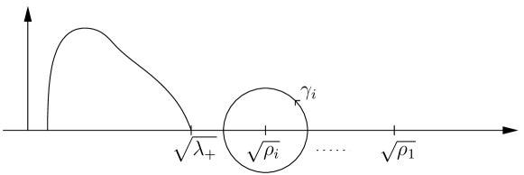
Figure 1: The contour $\gamma_{i}$ w.r.t. the support of the limit singular value distribution of $X_{n}$ and the other $\sqrt{\rho_{\ell}}$.

The approximation $b_{1}^{*}\widehat{\Pi}_{i}b_{2}\simeq T_{i}$ will be justified rigorously below. For the moment, let us develop the expression of $T_{i}$. Defining the $r\times r$ matrices:

$${\mathcal{I}}_{i}=\begin{bmatrix}0&&\\ &I_{j_{i}}&\\ &&0\end{bmatrix}\ ,$$

where the integers $j_{i}$ are defined in Assumption A5, we have

$$H(z)^{-1}=\sum_{i=1}^{s}\frac{1}{z^{2}m(z^{2})\tilde{m}(z^{2})\omega_{i}^{2}-1}\begin{bmatrix}z\tilde{m}(z^{2})\omega_{i}^{2}&-1\\ -1&zm(z^{2})\end{bmatrix}\otimes{\mathcal{I}}_{i}\ ,$$ (11)

which leads to

$$T_{i} =\frac{1}{\imath\pi}\sum_{\ell=1}^{s}b_{1}^{*}\Pi_{\ell}b_{2}\oint_{\gamma_{i}}\frac{z^{3}m(z^{2})^{2}\tilde{m}(z^{2})\omega_{\ell}^{2}}{z^{2}m(z^{2})\tilde{m}(z^{2})\omega_{\ell}^{2}-1}\,dz$$

$$=\frac{1}{2\imath\pi}\sum_{\ell=1}^{s}b_{1}^{*}\Pi_{\ell}b_{2}\oint_{\gamma_{i}^{\prime}}\frac{wm(w)^{2}\tilde{m}(w)\omega_{\ell}^{2}}{wm(w)\tilde{m}(w)\omega_{\ell}^{2}-1}\,dw$$

by making the change of variable $w=z^{2}$. Observe that the path $\gamma_{i}^{\prime}$ now encloses $\rho_{i}$ only. Recall that $wm(w)\tilde{m}(w)\omega_{\ell}^{2}-1=0$ if and only if $w=\rho_{\ell}$ for every $\ell$ such that $\omega_{\ell}^{2}>1/g(\lambda_{+}^{+})$, and since $g(w)=wm(w)\tilde{m}(w)$ is decreasing on $(\lambda_{+},\infty)$, these zeros are simple. As a result, the integrals above are equal to zero for $\ell\neq i$, and the integrand has a simple pole at $w=\rho_{i}$ for $\ell=i$. By the Residue Theorem, we have:

$$T_{i}=\frac{1}{\imath\pi}\oint_{\gamma_{i}}a_{1}^{*}(z)H(z)^{-1}a_{2}(z)\,dz=\frac{\rho_{i}m(\rho_{i})^{2}\tilde{m}(\rho_{i})}{(\rho_{i}m(\rho_{i})\tilde{m}(\rho_{i}))^{\prime}}b_{1}^{*}\Pi_{i}b_{2}$$ (12)

where the denominator at the right hand side is the derivative of the function $\lambda\mapsto\lambda m(\lambda)\tilde{m}(\lambda)$ at $\lambda=\rho_{i}$. We now make this argument more rigorous:

Theorem 2.

Let Assumptions A1-A5 hold true. For a given $i\leq s$, assume that $\omega_{i}^{2}>1/g(\lambda_{+}^{+})$. Let $(b_{1,n})$ and $(b_{2,n})$ be two sequences of deterministic vectors with bounded norms. Then

$$b_{1,n}^{*}\widehat{\Pi}_{i,n}b_{2,n}-\frac{\rho_{i}m(\rho_{i})^{2}\tilde{m}(\rho_{i})}{(\rho_{i}m(\rho_{i})\tilde{m}(\rho_{i}))^{\prime}}b_{1,n}^{*}\Pi_{i,n}b_{2,n}\xrightarrow[n\to\infty]{\text{a.s.}}0\ .$$

Proof.

Write

$$\widehat{T}_{i}=\frac{1}{\imath\pi}\oint_{\gamma_{i}}\hat{a}_{1}^{*}(z)\widehat{H}(z)^{-1}\hat{a}_{2}(z)\,dz\ .$$

Then, with probability one, $b_{1}^{*}\widehat{\Pi}_{i}b_{2}=\widehat{T}_{i}$ for $n$ large enough. Indeed, on the set $O_{n}$ (as defined in (3)), the singular values of $\Sigma$ greater than $\sqrt{\lambda_{+}}+\varepsilon_{1}$ coincide with the poles of $\widehat{H}(z)$ which are greater than $\sqrt{\lambda_{+}}+\varepsilon_{1}$ by the argument preceding Theorem 1. On this set, the first integral on the right hand side (r.h.s.) of (9) is zero, and by Theorem 1, the second integral can be replaced with $\int_{\gamma_{i}}$ with probability one for $n$ large enough. By Lemma 5, the differences $\widehat{H}(z)-H(z)$, $\hat{a}_{1}(z)-a_{1}(z)$, and $\hat{a}_{2}(z)-a_{2}(z)$ a.s. converge to zero, uniformly on $\gamma_{i}$. Hence $\widehat{T}_{i}-T_{i}\xrightarrow{\text{a.s.}}0$. ∎

4 The Spike MUSIC Estimation Algorithm

Algorithm description

We now consider the application context described in the introduction, and assume that $P_{n}=B_{n}(\varphi_{1},\ldots,\varphi_{r})S_{n}^{*}$ where $B_{n}(\varphi_{1},\ldots,\varphi_{r})=\begin{bmatrix}b_{n}(\varphi_{1})\cdots b_{n}(\varphi_{k})\end{bmatrix}$, and $b_{n}(\varphi)=N^{-1/2}\begin{bmatrix}\exp(-\imath D\ell\varphi)\end{bmatrix}_{\ell=0}^{N-1}$ with domain $\varphi\in[0,\pi/D]$. When the $\varphi_{k}$ are different, one can check that $B_{n}^{*}B_{n}\to I_{r}$ as $n\to\infty$. In most practical cases of interest, $S_{n}^{*}S_{n}\to O^{2}$ where $O$ is given by Equation (2). In these conditions, due to $B_{n}^{*}B_{n}\to I_{r}$, the diagonal elements of $O$ are the limits of the singular values of $P_{n}$ and Assumption A5 holds true.

In the area of signal processing, the positive real numbers $\omega_{i}^{2}$ are called the Signal to Noise Ratios (SNR) associated with the $r$ sources. Assumption A5 becomes:

Assumption A6.

Matrices $P_{n}$ of dimension $N\times n$ are deterministic and are written:

$$P_{n}=B_{n}(\varphi_{1},\cdots\varphi_{r})S_{n}^{*}$$

where $r$ is a fixed integer, $B_{n}(\varphi_{1},\cdots\varphi_{r})=\begin{bmatrix}b_{n}(\varphi_{1})&\cdots&b_{n}(\varphi_{r})\end{bmatrix}$ is a $N\times r$ matrix, $b_{n}(\varphi)=N^{-1/2}\begin{bmatrix}\exp(-\imath D\ell\varphi)\end{bmatrix}_{\ell=0}^{N-1}$ on $\varphi\in[0,\pi/D]$, and the $\varphi_{k}$ are all different. Matrix $S_{n}$ of dimensions $n\times r$ satisfies:

$$\sqrt{n}(S_{n}^{*}S_{n}-O^{2})={\mathcal{O}}(1)$$

as $n\to\infty$, where $O$ is defined in Assumption A5, and ${\mathcal{O}}$ is the classical Landau notation.

The assumption over the speed of convergence of $S^{*}S$ will be needed only for the purpose of the second order analysis. It is satisfied by most practical systems met in the field of signal processing. We moreover observe that it is possible to relax the assumption that $O$ is diagonal at the expense of a more complicated second order analysis.

In order for the algorithm to be able to estimate the $r$ angles, it is necessary that the perturbation $P$ gives rise to $r$ isolated eigenvalues, a fact that is stated in the following assumption:

Assumption A7.

Recall the definition (6) of function $g$, let $\lambda_{+}$ as defined in A3 and let $g(\lambda_{+}^{+})=\lim_{x\downarrow\lambda_{+}}g(x)$. Let the $\omega_{i}$’s as defined in A5, then:

$$\omega_{r}^{2}>\frac{1}{g(\lambda_{+}^{+})}\ .$$

The Spike MUSIC algorithm goes like this. The localization function $\chi(\varphi)$ defined in the introduction is also written as $\chi(\varphi)=\sum_{i=1}^{s}b(\varphi)^{*}\Pi_{i}b(\varphi)$. Given $\varphi$, the results of the previous section (Theorems 1 and 2 with $b_{1}=b_{2}=b(\varphi)$) show us that:

$$\hat{\chi}_{n}(\varphi)=\sum_{k=1}^{r}|b_{n}(\varphi)^{*}\hat{u}_{k,n}|^{2}\zeta(\hat{\lambda}_{k,n})\ ,$$ (13)

where

$$\zeta(\lambda)=\frac{(\lambda m(\lambda)\tilde{m}(\lambda))^{\prime}}{\lambda m(\lambda)^{2}\tilde{m}(\lambda)}$$ (14)

is a consistent estimator of $\chi_{n}(\varphi)$ in the asymptotic regime described by A1. By searching for the maxima of $\hat{\chi}(\varphi)$, we infer that we obtain consistent estimates of the angles or arrival. Observe that this algorithm requires the knowledge of the Stieltjes Transform of the limit spectral measure of $XX^{*}$ (available if the statistical description of the noise is known) and the number $r$ of emitting sources. Notice that when this number is unknown, it can be estimated along the ideas described in e.g. [10, 22].
We now perform the first order analysis of this algorithm.

First order analysis of the Spike MUSIC algorithm

We now formalize the argument of the previous paragraph and we push it further to show the consistency “up to the order $n$” of the Spike MUSIC estimator. We shall need this speed to perform the second order analysis (Lemma 9 below).

Theorem 3.

Let Assumptions A1-A6 hold true. Then for all $k=1,\cdots,r$, there exists a local maximum $\hat{\varphi}_{k,n}$ of $\hat{\chi}_{n}(\varphi)$ such that

$$n(\hat{\varphi}_{k,n}-\varphi_{k})\xrightarrow[n\to\infty]{\text{a.s.}}0.$$

The proof of this theorem is performed in two steps. With an approach similar to the one used in Section 3, we first prove that $\hat{\chi}(\varphi)-\chi(\varphi)\xrightarrow{\text{a.s.}}0$, and the convergence is uniform on $\varphi\in[0,\pi/D]$ (Proposition  1 below). Next, following the technique of [16, 17], we prove that this uniform a.s. convergence leads to Theorem 3.

In the sequel, we write:

$$\hat{a}(z,\varphi) = \begin{bmatrix}zU^{*}Q(z^{2})\\ \Omega V^{*}\widetilde{Q}(z^{2})X^{*}\end{bmatrix}b(\varphi)\quad\text{and}\quad a(z,\varphi)\ =\ \begin{bmatrix}zm(z^{2})U^{*}\\ 0\end{bmatrix}b(\varphi)\ ,$$ (15)

$$\hat{a}^{*}(z,\varphi) = b^{*}(\varphi)[zQ(z^{2})U\quad X\widetilde{Q}(z^{2})V\Omega]\ ,$$

$$a^{*}(z,\varphi) = b(\varphi)[zm(z^{2})U\quad 0]\ .$$

Beware that $\hat{a}^{*}$ and $a^{*}$ are not the Hermitian adjoints of $\hat{a}$ and $a$ (see the footnote associated to Eq. (10)).

Proposition 1.

In the setting of Theorem 3,

$$\max_{\varphi\in[0,\pi/D]}\left|\hat{\chi}_{n}(\varphi)-\chi_{n}(\varphi)\right|\xrightarrow[n\to\infty]{\text{a.s.}}0\ .$$

Proof.

Write

$$\hat{\chi}(\varphi)-\chi(\varphi)=\sum_{k=1}^{r}(\zeta(\hat{\lambda}_{k})-\zeta(\rho_{i(k)}))|b(\varphi)^{*}\hat{u}_{k}|^{2}+\sum_{i=1}^{s}\left(\zeta(\rho_{i})b(\varphi)^{*}\widehat{\Pi}_{i}b(\varphi)-b(\varphi)^{*}\Pi_{i}b(\varphi)\right).$$

By Theorem 1 and the continuity of $\zeta$ on $(\lambda_{+},+\infty)$, the first term at the r.h.s. goes to zero a.s. and uniformly in $\varphi$. Consider the second term. Let $\gamma_{i}$ be a small enough positively oriented circle which does not meet $\operatorname*{supp}(\pi)\cup\{\sqrt{\rho_{1}},\cdots,\sqrt{\rho_{s}}\}$ and such that only $\sqrt{\rho_{i}}\in\operatorname*{Int}(\gamma_{i})$. Since $\hat{\lambda}_{k}\xrightarrow{\text{a.s.}}\rho_{i(k)}$,

$$\max_{i}\max_{\varphi}\left|b(\varphi)^{*}\widehat{\Pi}_{i}b(\varphi)-\widehat{T}_{i}(\varphi)\right|=0$$

a.s. for $n$ large enough, where

$$\widehat{T}_{i}(\varphi)=\frac{1}{\imath\pi}\oint_{\gamma_{i}}\hat{a}^{*}(z,\varphi)\widehat{H}(z)^{-1}\hat{a}(z,\varphi)\,dz$$

Recalling Eq. (12), it will therefore be enough to prove that

$$\max_{1\leq i\leq s}\max_{\varphi\in[0,\pi/D]}|Z_{i}(\varphi)|\xrightarrow[n\to\infty]{a.s.}0\ ,$$

where

$$Z_{i}(\varphi)=\frac{1}{\imath\pi}\oint_{\gamma_{i}}\left(\hat{a}^{*}(z,\varphi)\widehat{H}(z)^{-1}\hat{a}(z,\varphi)-a^{*}(z,\varphi)H(z)^{-1}a(z,\varphi)\right)\,dz\ .$$

We have

$$\max_{\varphi}|Z_{i}(\varphi)|\leq 2R\int_{0}^{1}\max_{\varphi}e(\sqrt{\rho_{i}}+Re^{2\imath\pi\theta},\varphi)\,d\theta$$

where $R$ is the radius of $\gamma_{i}$ and where

$$e(z,\varphi) =\left|\hat{a}^{*}(z,\varphi)\widehat{H}(z)^{-1}\hat{a}(z,\varphi)-a^{*}(z,\varphi)H(z)^{-1}a(z,\varphi)\right|.$$

$$\leq\left|(\hat{a}^{*}-a^{*})H^{-1}\hat{a}\right|+\left|aH^{-1}(\hat{a}-a)\right|+\left|\hat{a}^{*}(\widehat{H}^{-1}-H^{-1})\hat{a}\right|.$$

Since $\|H^{-1}\|$, $\max_{\varphi}\|a\|$ and $\max_{\varphi}\|\hat{a}\|$ are bounded on $\gamma_{i}$, $e(z,\varphi)$ satisfies on this path

$$e(z,\varphi)\leq K\left(\|\hat{a}(z,\varphi)-a(z,\varphi)\|+\|\widehat{H}(z)^{-1}-H(z)^{-1}\|\right)\ .$$

By Lemma 5 and the fact that $\|H^{-1}\|$ is bounded on $\gamma_{i}$, the term $\|\widehat{H}^{-1}-H^{-1}\|=\|\widehat{H}^{-1}(H-\widehat{H})H^{-1}\|$ converges to zero uniformly on $\gamma_{i}$ with probability one. To obtain the result, we prove that $\|\hat{a}-a\|\xrightarrow{\text{a.s.}}0$ and that this convergence is uniform on $(z,\varphi)\in\gamma_{i}\times[0,\pi/D]$. Let us focus on the first term $zu_{1}^{*}(Q(z^{2})-m(z^{2})I)b(\varphi)$ of $\hat{a}-a$, where we recall that $u_{1}$ is the first column of $U$. Since $\|b(\varphi)\|=\|u_{1}\|=1$,

$$|zu_{1}^{*}(Q(z^{2})-m(z^{2})I)b(\varphi)|\leq|zu_{1}^{*}(Q(z^{2})-\alpha(z^{2})I)b(\varphi)|+|z(\alpha(z^{2})-m(z^{2}))|\ .$$

With probability one, the second term converges to zero on $\gamma_{i}$, and the convergence is uniform (along the principle of the proof of Lemma 5). Since

$$\sup_{n}\max_{\varphi}\|n^{-1}b^{\prime}(\varphi)\|=\sup_{n}\max_{\varphi}\left\|n^{-1}N^{-1/2}\begin{bmatrix}\ell D\exp(-\imath\ell D\varphi)\end{bmatrix}_{\ell=0}^{N-1}\right\|<\infty\ ,$$

the term

$$\xi(z,\varphi)={\mathbbm{1}}_{O_{n}}\times zu_{1}^{*}(Q(z^{2})-\alpha(z^{2})I)b(\varphi)$$

satisfies

$$|\xi(z_{1},\varphi_{1})-\xi(z_{2},\varphi_{2})|\leq K(n|\varphi_{1}-\varphi_{2}|+|z_{1}-z_{2}|)$$

for every $(z_{1},\varphi_{1})$, $(z_{2},\varphi_{2})$ in $\gamma_{i}\times[0,\pi/D]$. Therefore, it will be enough to prove that

$$\max_{(z,\varphi)\in A_{n}\times B_{n}}\xi(z,\varphi)\xrightarrow[n\to\infty]{\text{a.s.}}0$$

where $A_{n}$ contains $n$ regularly spaced points in $\gamma_{i}$ and $B_{n}$ contains $n^{2}$ regularly spaced points in $[0,\pi/D]$. This can be obtained from Lemma 3 with $p=9$, Markov inequality and Borel Cantelli’s lemma. The other terms of $\hat{a}-a$ can be handled similarly. ∎

We now prove Theorem 3 by following the ideas of [16, 17]. To that end, we need the following lemma, proven in [14]:

Lemma 7.

Let $(c_{N})$ be a sequence of real numbers belonging to a compact of $[-1/2,1/2]$ and converging to $c$. Let

$$q_{N}(c_{N})=\frac{1}{N}\sum_{k=0}^{N-1}\exp(-2\imath\pi kc_{N})\ .$$

Then the following hold true:

$$q_{N}(c_{N}) \xrightarrow[N\to\infty]{} 0\quad\text{if}\ c\neq 0\ ,$$

$$q_{N}(c_{N}) \xrightarrow[N\to\infty]{} 0\quad\text{if}\ c=0\ \text{and}\ N|c_{N}-c|\to\infty\ ,$$

$$q_{N}(c_{N}) \xrightarrow[N\to\infty]{} \exp(-\imath\pi d)\operatorname*{sinc}(d)\quad\text{if}\ c=0\ \text{and}\ N|c_{N}-c|\to d\ ,$$

where $\operatorname*{sinc}$ stands as usual for sine cardinal.

Proof of Theorem 3.

We start by observing that $\chi(\varphi)=d(\varphi)^{*}(B^{*}B)^{-1}d(\varphi)$ where $B$ is the matrix defined in A6 and where $d(\varphi)=\begin{bmatrix}b(\varphi_{k})^{*}b(\varphi)\end{bmatrix}_{k=1}^{r}$. By Lemma 7, $B^{*}B\to I_{r}$, hence $\chi(\varphi)-\|d(\varphi)\|^{2}\to 0$.

In the remainder of the proof, we shall stay in the probability one set where the uniform convergence in the statement of Proposition 1 holds true. Taking $k=1$ without loss of generality, we shall show that any sequence $\hat{\varphi}_{1,n}$ for which $\hat{\chi}(\hat{\varphi}_{1,n})$ attains its maximum in the closure of a small neighborhood of $\varphi_{1}$ satisfies $N(\hat{\varphi}_{1,n}-\varphi_{1})\to 0$. Given a sequence of such $\hat{\varphi}_{1,n}$, assume we can extract a subsequence $\hat{\varphi}_{1,n^{*}}$ such that $N|\hat{\varphi}_{1,n^{*}}-\varphi_{1}|\to\infty$. In this case, Lemma 7 and the observations made above on the structure of $\chi(\varphi)$ show that $\chi(\hat{\varphi}_{1,n^{*}})\to 0$. Since $\max_{\varphi}|\hat{\chi}(\varphi)-\chi(\varphi)|\to 0$, $\hat{\chi}(\hat{\varphi}_{1,n^{*}})\to 0$. But $\hat{\chi}(\varphi_{1})\to\chi(\varphi_{1})=1$, which contradicts the fact that $\hat{\varphi}_{1,n^{*}}$ maximizes $\hat{\chi}$. Hence the sequence $N(\hat{\varphi}_{1,n^{*}}-\varphi_{1})$ belongs to a compact. Assume $N(\hat{\varphi}_{1,n^{*}}-\varphi_{1})\not\to 0$. If we take a further subsequence of the latter that converges to a constant $d\neq 0$, then by Lemma 7, $\hat{\chi}$ converges to $\operatorname*{sinc}(d)^{2}<1$ along this subsequence, which also raises a contradiction. This proves the theorem.∎

5 Second Order Analysis of the Spike MUSIC Estimator

In order to perform the second order analysis, we also assume:

Assumption A8.

Let $\lambda_{-}$, $\lambda_{+}$, $\alpha$ and $m$ be as in A3. Then for any $z\in{\mathbb{C}}-[\lambda_{-},\lambda_{+}]$, $\sqrt{n}\left(\alpha(z)-m(z)\right)$ converges in probability to zero.

Remark 2.

If $\sqrt{n}X$ is standard Gaussian and if $c_{n}=N/n$ satisfies $\sqrt{n}(c_{n}-c)\to 0$, then Assumption A8 is satisfied. Indeed, call $m_{n}(z)$ the Stieltjes Transform of the Marčenko-Pastur distribution, i.e., the analytic continuation of (7), when $c$ is replaced with $c_{n}$, and let $\pi_{n}$ be the associated probability measure. For $z\in{\mathbb{C}}-[\lambda_{-},\lambda_{+}]$, function $f(x)=(x-z)^{-1}$ is analytic outside the support of $\pi_{n}$ for $n$ large, and [3, Th.1.1] can be applied to show that $\sqrt{n}(\alpha_{n}(z)-m_{n}(z))\xrightarrow{\mathcal{P}}0$. When $\sqrt{n}(c_{n}-c)\to 0$, it is furthermore clear that $\sqrt{n}(m_{n}(z)-m(z))\to 0$.

The main result of this section is the following:

Theorem 4.

Let Assumptions A1-A8 hold true. Then the estimates $\hat{\varphi}_{k,n}$ satisfy

$$n^{3/2}\begin{bmatrix}\hat{\varphi}_{1,n}-\varphi_{1}\\ \vdots\\ \hat{\varphi}_{r,n}-\varphi_{r}\end{bmatrix}\xrightarrow[n\to\infty]{{\mathcal{D}}}{\mathcal{N}}\left(0,\begin{bmatrix}\sigma_{1}^{2}I_{j_{1}}&&\\ &\ddots&\\ &&\sigma_{s}^{2}I_{j_{s}}\end{bmatrix}\right)$$ (16)

where

$$\sigma_{i}^{2}=\frac{6}{c^{2}D^{2}}\left(\frac{m^{\prime}(\rho_{i})-m(\rho_{i})^{2}}{cm(\rho_{i})^{2}}+\omega_{i}^{2}\left(m(\rho_{i})+\rho_{i}m^{\prime}(\rho_{i})\right)\right),\quad 1\leq i\leq s\ .$$

When $\sqrt{n}X$ is standard Gaussian, plugging the r.h.s. of (7) into this expression leads after some derivations to:

Corollary 2.

If $\sqrt{n}X$ is standard Gaussian and if $\sqrt{n}(c_{n}-c)\to 0$, the convergence (16) holds true with

$$\sigma_{i}^{2}=\frac{6}{c^{2}D^{2}}\frac{\omega_{i}^{2}+1}{\omega_{i}^{4}-c}.$$

This corollary calls for some comments:

Remark 3 (Efficiency at high SNR).

Recalling that $\omega_{i}^{2}>\sqrt{c}$ is the condition for the existence of a corresponding isolated eigenvalue (Corollary 1), we observe that the estimator variance for $\varphi_{k}$ goes to infinity as the corresponding $\omega_{i}^{2}$ decreases to $\sqrt{c}$. At the other extreme, this variance behaves like $6c^{-2}D^{-2}\omega_{i}^{-2}$ as $\omega_{i}^{2}\to\infty$. It is useful to notice that this asymptotic variance coincides with the Cramér-Rao bound for estimating $\varphi_{k}$ [28]. In other words, the Spike MUSIC estimator is efficient at high SNR when the noise matrix is standard Gaussian.

A numerical illustration

In order to illustrate the convergence and the fluctuations of the Spike MUSIC algorithm, we simulate a radio signal transmission satisfying Assumptions A1-A8. We consider $r=2$ emitting sources located at the angles $0.5$ and $1$ radian, and a number of receiving antennas ranging from $N=5$ to $N=50$. The observation window length is set to $n=2N$ (hence $c=0.5$). The noise matrix $X_{n}$ is such that $\sqrt{n}X_{n}$ is standard Gaussian. The source powers are assumed equal, so that the matrix $O$ given by Equation (2) is written $O=\omega I_{2}$, and the Signal to Noise Ratio for any source is $\text{SNR}=10\log_{10}\omega^{2}$ decibels. In Figure 2, the SNR is set to $10$ dB, and the empirical variance of $\hat{\varphi}_{1,n}-\varphi_{1}$ (red curve) is computed over $2000$ runs. The variance provided by Corollary 2 is also plotted versus $N$. We observe a good fit between the variance predicted by Corollary 2 and the empirical variance after $N=15$ antennas.

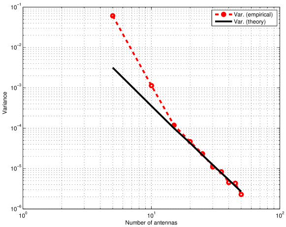
Figure 2: Spike MUSIC algorithm, Variance vs $N$.

In Figure 3, the variance is plotted as a function of the SNR, the number of antennas being fixed to $N=20$. The empirical variance is computed over $5000$ runs. The Cramér-Rao Bound is also plotted. The empirical variance fits the theoretical one from $\text{SNR}\approx 6$ dB upwards.

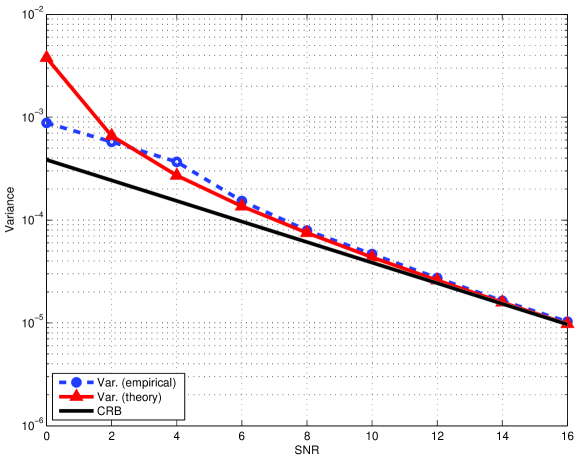
Figure 3: Spike MUSIC algorithm, Variance vs the SNR.

Proof of Theorem 4.

We start with some additional notations and definitions. Matrix $B=\begin{bmatrix}b(\varphi_{1}),\ldots,b(\varphi_{r})\end{bmatrix}$ will be often written as $B=[b_{1},\ldots,b_{r}]$ or in block form as $B=\begin{bmatrix}B_{1},\ldots,B_{s}\end{bmatrix}$ where $B_{i}$ has $j_{i}$ columns. We shall also write $B^{\prime}=\begin{bmatrix}b^{\prime}(\varphi_{1}),\ldots,b^{\prime}(\varphi_{r})\end{bmatrix}$ and $B^{\prime\prime}=\begin{bmatrix}b^{\prime\prime}(\varphi_{1}),\ldots,b^{\prime\prime}(\varphi_{r})\end{bmatrix}$ where $b^{\prime}(\varphi)$ and $b^{\prime\prime}(\varphi)$ are respectively the first and second derivatives of $b(\varphi)$. We shall also use the short hand notations $B^{\prime}=[b_{1}^{\prime},\ldots,b_{r}^{\prime}]$ and $B^{\prime\prime}=[b_{1}^{\prime\prime},\ldots,b_{r}^{\prime\prime}]$. Matrix $B^{\perp}=[b_{1}^{\perp},\ldots,b_{r}^{\perp}]$ will be defined by the equation

$$\frac{1}{n}B^{\prime}=-\frac{\imath cD}{2}B+\frac{cD}{2\sqrt{3}}B^{\perp}.$$ (17)

Finally, if $x_{n},y_{n}$ are random sequences, we denote by $x_{n}\asymp y_{n}$ the convergence $x_{n}-y_{n}\xrightarrow[]{\mathcal{P}}0$.

We now state some preliminary results. In the following, we say that the complex random vector $\eta$ is governed by the law ${\cal CN}(0,R)$ where $R$ is a nonnegative Hermitian matrix if the real vector $\begin{bmatrix}\Re(\eta)\\ \Im(\eta)\end{bmatrix}$ has the law ${\cal N}\Bigl{(}0,\frac{1}{2}\begin{bmatrix}\Re(R)&-\Im(R)\\ \Im(R)&\Re(R)\end{bmatrix}\Bigr{)}$. The following proposition, whose proof is postponed to A, is crucial:

Proposition 2.

Let Assumptions A1-A4 hold true. Let $t\leq N$ be a fixed integer, let $W=\begin{bmatrix}w_{1},\cdots,w_{t}\end{bmatrix}$ and $\widetilde{W}=\begin{bmatrix}\tilde{w}_{1},\cdots,\tilde{w}_{t}\end{bmatrix}$ be deterministic isometry matrices with dimensions $N\times t$ and $n\times t$ respectively. Let $\rho$ be a real number such that $\rho>\lambda_{+}$. Then

$$\xi_{n}=\sqrt{n}\left(W^{*}\Bigl{(}Q(\rho)-\alpha(\rho)I_{N}\Bigr{)}W,\ \widetilde{W}^{*}\Bigl{(}\widetilde{Q}(\rho)-\tilde{\alpha}(\rho)I_{n}\Bigr{)}\widetilde{W},\ W^{*}X\widetilde{Q}(\rho)\widetilde{W}\right)$$

is tight.

Assume $t$ is even. Given real numbers $\rho_{1},\ldots,\rho_{t/2}$ all strictly greater than $\lambda_{+}$, the $t\times 1$ random vector

$$\eta_{n}=\left[\sqrt{N}\left(w_{k}^{*}Q(\rho_{k})w_{t/2+k}\right)_{1\leq k\leq t/2},\sqrt{n}\left(w_{k}^{*}X\widetilde{Q}(\rho_{k})\tilde{w}_{k}\right)_{1\leq k\leq t/2}\right]^{T}$$

converges in distribution towards $\mathcal{CN}(0,R)$ with

$$R=\begin{bmatrix}\operatorname*{diag}\left(m^{\prime}(\rho_{k})-m(\rho_{k})^{2}\right)_{k=1}^{t/2}&0\\ 0&\operatorname*{diag}\left(m(\rho_{k})+\rho_{k}m^{\prime}(\rho_{k})\right)_{k=1}^{t/2}\end{bmatrix}.$$

Writing $Q-mI=(Q-\alpha I)+(\alpha-m)I$, and similarly for $\widetilde{Q}$, we obtain:

Corollary 3.

Assume in addition that Assumption A8 is satisfied. Then

$$\xi_{n}=\sqrt{n}\left(W^{*}\Bigl{(}Q(\rho)-m(\rho)I_{N}\Bigr{)}W,\ \widetilde{W}^{*}\Bigl{(}\widetilde{Q}(\rho)-\tilde{m}(\rho)I_{n}\Bigr{)}\widetilde{W},\ W^{*}X\widetilde{Q}(\rho)\widetilde{W}\right)$$

is tight.

Intuitively, tightness of $\xi_{n}$ leads to the tightness of the $\sqrt{n}(\hat{\lambda}_{k,n}-\rho_{i(k)})$. This is formalized by the following proposition, proven in B:

Proposition 3.

Assume the setting of Theorem 4. Then the sequences $\sqrt{n}(\hat{\lambda}_{k,n}-\rho_{i(k)})$ are tight for $1\leq k\leq r$.

The following lemma is proven in C.

Lemma 8.

Let Assumptions A5 and A6 hold true. Then the following convergences hold true:

$$B^{*}B \xrightarrow[n\to\infty]{} I_{r}\ ,$$

$$\frac{1}{n^{2}}B^{*}B^{\prime\prime} \xrightarrow[n\to\infty]{} -\left(\frac{c^{2}D^{2}}{3}\right)I_{r}\ ,$$

$$(B^{\perp})^{*}B^{\perp} \xrightarrow[n\to\infty]{} I_{r}\ ,$$

$$(B^{\perp})^{*}B \xrightarrow[n\to\infty]{} 0\ ,$$

$$\|\Pi_{i}-\Pi_{B_{i}}\| \xrightarrow[n\to\infty]{} 0\ \text{for all }i=1,\ldots,s$$

where $\Pi_{B_{i}}$ is the orthogonal projection matrix on the column space of $B_{i}$.

We now enter the proof of Theorem 4.

Recall the definitions (13) and (14) of $\hat{\chi}$ and $\zeta$. In most of the proof, we shall focus on $\sqrt{n}(\hat{\varphi}_{1,n}-\varphi_{1})$. Recalling that $\hat{\chi}^{\prime}(\hat{\varphi}_{1})=0$ and performing a Taylor-Lagrange expansion of $\hat{\chi}^{\prime}$ around $\varphi_{1}$, we obtain

$$0=\hat{\chi}^{\prime}(\hat{\varphi}_{1})=\hat{\chi}^{\prime}(\varphi_{1})+(\hat{\varphi}_{1}-\varphi_{1})\hat{\chi}^{\prime\prime}(\varphi_{1})+\frac{(\hat{\varphi}_{1}-\varphi_{1})^{2}}{2}\hat{\chi}^{(3)}(\bar{\varphi}_{1})\ ,$$

where $\hat{\chi}^{(3)}$ is the third derivative of $\hat{\chi}$ and where $\bar{\varphi}_{1}\in[\varphi_{1}\wedge\hat{\varphi}_{1},\varphi_{1}\vee\hat{\varphi}_{1}]$. Hence

$$n^{3/2}(\hat{\varphi}_{1}-\varphi_{1})=-\frac{n^{-1/2}\hat{\chi}^{\prime}(\varphi_{1})}{n^{-2}\hat{\chi}^{\prime\prime}(\varphi_{1})+0.5n^{-2}(\hat{\varphi}_{1}-\varphi_{1})\hat{\chi}^{(3)}(\bar{\varphi}_{1})}\ .$$

We start by characterizing the asymptotic behavior of the denominator of this equation:

Lemma 9.

Assume that the setting of Theorem 4 holds true. Then,

$$\frac{\hat{\chi}^{\prime\prime}(\varphi_{1})}{n^{2}}+(\hat{\varphi}_{1}-\varphi_{1})\frac{\hat{\chi}^{(3)}(\bar{\varphi}_{1})}{2n^{2}}\xrightarrow[n\to\infty]{\text{a.s.}}-\frac{c^{2}D^{2}}{6}\ .$$

Proof.

We have

$$\frac{\hat{\chi}^{\prime\prime}(\varphi_{1})}{n^{2}} = \frac{2}{n^{2}}\sum_{k=1}^{r}\zeta(\hat{\lambda}_{k})|(b^{\prime}_{1})^{*}\widehat{u}_{k}|^{2}+\frac{2}{n^{2}}\sum_{k=1}^{r}\Re\left(\zeta(\hat{\lambda}_{k})b_{1}^{*}\widehat{u}_{k}\widehat{u}_{k}^{*}b^{\prime\prime}_{1}\right)\ ,$$

$$\frac{\chi^{\prime\prime}(\varphi_{1})}{n^{2}} = \frac{2}{n^{2}}(b^{\prime}_{1})^{*}UU^{*}b^{\prime}_{1}+\frac{2}{n^{2}}\Re\left(b_{1}^{*}UU^{*}b^{\prime\prime}_{1}\right)\ .$$ (18)

Theorem 1 along with the continuity of $\zeta$ on $(\lambda_{+},\infty)$, and Theorem 2 show that

$$\frac{1}{n^{2}}\hat{\chi}^{\prime\prime}(\varphi_{1})-\frac{1}{n^{2}}\chi^{\prime\prime}(\varphi_{1})\xrightarrow[n\to\infty]{a.s.}0\ .$$

Writing

$$\frac{1}{n^{2}}\chi^{\prime\prime}(\varphi_{1})=\frac{2}{n^{2}}\sum_{i=1}^{s}\left((b^{\prime}_{1})^{*}\Pi_{i}b^{\prime}_{1}+\Re(b_{1}^{*}\Pi_{i}b^{\prime\prime}_{1})\right),$$

we have

$$\frac{1}{n^{2}}(b^{\prime}_{1})^{*}\Pi_{i}b^{\prime}_{1} = \left(-\frac{\imath cD}{2}b_{1}+\frac{cD}{2\sqrt{3}}b_{1}^{\perp}\right)^{*}\Pi_{i}\left(-\frac{\imath cD}{2}b_{1}+\frac{cD}{2\sqrt{3}}b_{1}^{\perp}\right)\ ,$$

$$\xrightarrow[n\to\infty]{} \frac{c^{2}D^{2}}{4}\delta_{i,0}$$

by the first, fourth and fifth assertions of Lemma 8. By the same lemma,

$$\frac{1}{n^{2}}b_{1}^{*}\Pi_{i}b^{\prime\prime}_{1}-\frac{\delta_{i,0}}{n^{2}}b_{1}^{*}b^{\prime\prime}_{1}\ \to\ 0\quad\textrm{and}\quad\frac{1}{n^{2}}b_{1}^{*}b^{\prime\prime}_{1}\ \to\ -\frac{c^{2}D^{2}}{3}\ .$$

Hence $n^{-2}\hat{\chi}^{\prime\prime}(\varphi_{1})\to-c^{2}D^{2}/6$.

Furthermore, it is easily seen that $n^{-3}\hat{\chi}^{(3)}(\bar{\varphi}_{1})$ is bounded. Since $n(\hat{\varphi}_{1}-\varphi_{1})\xrightarrow{\text{a.s.}}0$ by Theorem 3, $n^{-2}(\hat{\varphi}_{1}-\varphi_{1})\hat{\chi}^{(3)}(\bar{\varphi}_{1})\xrightarrow{\text{a.s.}}0$, which establishes the result. ∎

We now turn to the numerator $n^{-1/2}\hat{\chi}^{\prime}(\varphi_{1})=2n^{-1/2}\sum_{k=1}^{r}\zeta(\hat{\lambda}_{k})\Re\left(b_{1}^{*}\hat{u}_{k}\hat{u}_{k}^{*}b^{\prime}_{1}\right)$, and start with the following lemma:

Lemma 10.

Assume that the setting of Theorem 4 holds true. Then

$$\frac{1}{\sqrt{n}}\hat{\chi}^{\prime}(\varphi_{1})-2\Re(\xi)\xrightarrow{\mathcal{P}}0\ ,$$

where

$$\xi=\sum_{i=1}^{s}\frac{\zeta(\rho_{i})}{\imath\pi\sqrt{n}}\oint_{\gamma_{i}}\left(\hat{a}^{*}(z,\varphi_{1})\widehat{H}(z)^{-1}\hat{a}^{\prime}_{\varphi}(z,\varphi_{1})-a^{*}(z,\varphi_{1})H(z)^{-1}a^{\prime}_{\varphi}(z,\varphi_{1})\right)dz,$$ (19)

and where the deterministic circle $\gamma_{i}$ encloses $\rho_{i}^{1/2}$ only and:

$$\hat{a}^{\prime}_{\varphi}(z,\varphi) = \frac{\partial\hat{a}(z,\varphi)}{\partial\varphi}=\begin{bmatrix}zU^{*}Q(z^{2})\\ \Omega V^{*}\widetilde{Q}(z^{2})X^{*}\end{bmatrix}b^{\prime}(\varphi)\ ,$$

$$a^{\prime}_{\varphi}(z,\varphi) = \frac{\partial a(z,\varphi)}{\partial\varphi}=\begin{bmatrix}zm(z^{2})U^{*}\\ 0\end{bmatrix}b^{\prime}(\varphi)\ .$$

Proof.

Recall the definition of $\hat{\chi}$ as given in (13). A direct computation yields:

$$\hat{\chi}^{\prime}(\varphi) = 2\sum_{k=1}^{r}\zeta(\hat{\lambda}_{k,n})\Re\left(b_{1}^{*}(\varphi)\hat{u}_{k}\hat{u}_{k}^{*}b^{\prime}_{1}(\varphi)\right)\ ,$$

$$= 2\sum_{i=1}^{s}\sum_{k:i(k)=i}\zeta(\hat{\lambda}_{k,n})\Re\left(b_{1}^{*}(\varphi)\hat{u}_{k}\hat{u}_{k}^{*}b^{\prime}_{1}(\varphi)\right)\ .$$

Recall that $r$ and $s$ are fixed and independent from $n$ by A5. We start by showing that

$$\frac{1}{\sqrt{n}}\hat{\chi}^{\prime}(\varphi_{1})-\frac{2}{\sqrt{n}}\sum_{i=1}^{s}\zeta(\rho_{i})\Re\left(b_{1}^{*}\widehat{\Pi}_{i}b^{\prime}_{1}\right)\xrightarrow[n\to\infty]{{\mathcal{P}}}0.$$ (20)

Since $\sqrt{n}(\zeta(\hat{\lambda}_{k,n})-\zeta(\rho_{i(k)}))$ is tight as a corollary of Proposition 3, it will be enough to prove that $n^{-1}\Re\left(b_{1}^{*}\hat{u}_{k}\hat{u}_{k}^{*}b^{\prime}_{1}\right)\to 0$ in probability for every $k$. By the definition (17) of $B^{\perp}$, we have

$$\frac{1}{n}\,\Re\left(b_{1}^{*}\hat{u}_{k}\hat{u}_{k}^{*}b^{\prime}_{1}\right)=\frac{cD}{2\sqrt{3}}\,\Re\left(b_{1}^{*}\hat{u}_{k}\hat{u}_{k}^{*}b_{1}^{\perp}\right)\ .$$

By Cauchy-Schwarz inequality,

$$\left|b_{1}^{*}\hat{u}_{k}\hat{u}_{k}^{*}b_{1}^{\perp}\right|^{2}\leq b_{1}^{*}\widehat{\Pi}_{i(k)}b_{1}\ (b_{1}^{\perp})^{*}\widehat{\Pi}_{i(k)}b_{1}^{\perp}.$$

By Theorem 2,

$$b_{1}^{*}\widehat{\Pi}_{i(k)}b_{1}\ (b_{1}^{\perp})^{*}\widehat{\Pi}_{i(k)}b_{1}^{\perp}\ -\ \zeta(\rho_{i(k)})^{-2}\ b_{1}^{*}\Pi_{i(k)}b_{1}\ (b_{1}^{\perp})^{*}\Pi_{i(k)}b_{1}^{\perp}\ \xrightarrow{\text{a.s.}}\ 0,$$

and by Lemma 8, $b_{1}^{*}\Pi_{i(k)}b_{1}\ (b_{1}^{\perp})^{*}\Pi_{i(k)}b_{1}^{\perp}\ \to\ 0$ (consider alternatively the cases $i(k)=1$ and $i(k)>1$) which proves (20).

Now, applying (9) and (15), and taking up an argument used in the proof of Theorem 2, we have

$$2\sum_{i=1}^{s}\frac{\zeta(\rho_{i})}{\sqrt{n}}\Re\left(b_{1}^{*}\widehat{\Pi}_{i}b^{\prime}_{1}\right) =2\sum_{i=1}^{s}\Re\left(\frac{-\zeta(\rho_{i})}{\imath\pi\sqrt{n}}\oint_{{\mathcal{C}}_{i}}\begin{bmatrix}b^{*}_{1}&0\end{bmatrix}{\bf Q}(z)\begin{bmatrix}b^{\prime}_{1}\\ 0\end{bmatrix}\ dz\right)$$

$$\phantom{=}+2\sum_{i=1}^{s}\Re\left(\frac{\zeta(\rho_{i})}{\imath\pi\sqrt{n}}\oint_{{\mathcal{C}}_{i}}\hat{a}^{*}(z,\varphi_{1})\widehat{H}(z)^{-1}\hat{a}^{\prime}_{\varphi}(z,\varphi_{1})\,dz\right)$$

$$=2\sum_{i=1}^{s}\Re\left(\frac{\zeta(\rho_{i})}{\imath\pi\sqrt{n}}\oint_{\gamma_{i}}\hat{a}^{*}(z,\varphi_{1})\widehat{H}(z)^{-1}\hat{a}^{\prime}_{\varphi}(z,\varphi_{1})\,dz\right)$$

with probability one for $n$ large. On the other hand, recalling (12), we have

$$0=\chi^{\prime}(\varphi_{1})=2\sum_{i=1}^{s}\Re\left(\frac{\zeta(\rho_{i})}{\imath\pi}\oint_{\gamma_{i}}a^{*}(z,\varphi_{1})H(z)^{-1}a^{\prime}_{\varphi}(z,\varphi_{1})\,dz\right)\ ,$$

which proves the result. ∎

Write $\widehat{H}(z)=H(z)+E(z)$ and $\hat{a}(z,\varphi)=a(z,\varphi)+e(z,\varphi)$. To be more specific,

$$E({z})=\begin{bmatrix}{z}U^{*}(Q(z^{2})-m(z^{2})I_{N})U&U^{*}X\widetilde{Q}(z^{2})V\Omega\\ \Omega V^{*}\widetilde{Q}(z^{2})X^{*}U&{z}\Omega V^{*}(\widetilde{Q}(z^{2})-\tilde{m}(z^{2})I_{n})V\Omega\end{bmatrix}$$ (21)

and

$$e(z,\varphi)=\begin{bmatrix}zU^{*}\left(Q(z^{2})-m(z^{2})I\right)\\ \Omega V^{*}\widetilde{Q}(z^{2})X^{*}\end{bmatrix}b(\varphi).$$

Write $e^{\prime}_{\varphi}(z,\varphi)=\partial e(z,\varphi)/\partial\varphi$. For a given $z\in\gamma_{i}$, $\widehat{H}^{-1}=H^{-1}-H^{-1}EH^{-1}+{\mathcal{O}}(\|E\|^{2})$. This suggests the following development

$$\xi =\sum_{i=1}^{s}\left(\frac{\zeta(\rho_{i})}{\imath\pi\sqrt{n}}\oint_{\gamma_{i}}a^{*}(z,\varphi_{1})H(z)^{-1}e^{\prime}_{\varphi}(z,\varphi_{1})\,dz\right.$$

$$\phantom{\sum_{i}^{s}}\quad+\frac{\zeta(\rho_{i})}{\imath\pi\sqrt{n}}\oint_{\gamma_{i}}e^{*}(z,\varphi_{1})H(z)^{-1}a^{\prime}_{\varphi}(z,\varphi_{1})\,dz$$

$$\phantom{\sum_{i}^{s}}\quad-\left.\frac{\zeta(\rho_{i})}{\imath\pi\sqrt{n}}\oint_{\gamma_{i}}a^{*}(z,\varphi_{1})H(z)^{-1}E(z)H(z)^{-1}a^{\prime}_{\varphi}(z,\varphi_{1})\,dz\ +q_{i}\right)$$

$$=\sum_{i=1}^{s}(X_{1,i}+X_{2,i}+X_{3,i}+q_{i})\ .$$

where the terms $q_{i}$ are “higher order terms” that appear when we expand the r.h.s. of (19). We first handle the terms $X_{k,i}$’s, then $q_{i}$.

The terms $X_{1,i}$

Writing $U_{n}=\begin{bmatrix}U_{1,n}\cdots U_{s,n}\end{bmatrix}$ and $V_{n}=\begin{bmatrix}V_{1,n}\cdots V_{s,n}\end{bmatrix}$ where both $U_{i,n}$ and $V_{i,n}$ have $j_{i}$ columns, and recalling (11), we have

$$X_{1,i} =\frac{\zeta(\rho_{i})}{\imath\pi\sqrt{n}}\sum_{\ell=1}^{s}\oint_{\gamma_{i}}\begin{bmatrix}zm(z^{2})b_{1}^{*}U_{\ell}&0\end{bmatrix}\times\frac{\begin{bmatrix}z\tilde{m}(z^{2})\omega_{\ell}^{2}&-1\\ -1&zm(z^{2})\end{bmatrix}\otimes I_{j_{\ell}}}{z^{2}m(z^{2})\tilde{m}(z^{2})\omega_{\ell}^{2}-1}\times$$

$$\ \ \ \ \ \ \ \ \ \ \ \ \ \ \ \ \ \ \ \ \ \ \ \ \ \ \ \ \ \ \ \ \ \ \ \ \ \ \ \ \ \ \ \ \ \ \ \ \ \ \ \ \ \ \ \ \ \ \ \ \ \ \ \ \begin{bmatrix}zU_{\ell}^{*}\left(Q(z^{2})-m(z^{2})I\right)b_{1}^{\prime}\\ \omega_{\ell}V_{\ell}^{*}\widetilde{Q}(z^{2})X^{*}b_{1}^{\prime}\end{bmatrix}\,dz$$

$$=\frac{\zeta(\rho_{i})}{\imath\pi\sqrt{n}}\sum_{\ell=1}^{s}\oint_{\gamma_{i}}\frac{z^{3}\omega_{\ell}^{2}m(z^{2})\tilde{m}(z^{2})b_{1}^{*}\Pi_{\ell}\left(Q(z^{2})-m(z^{2})I\right)b_{1}^{\prime}}{z^{2}m(z^{2})\tilde{m}(z^{2})\omega_{\ell}^{2}-1}\,dz$$

$$\ \ -\frac{\zeta(\rho_{i})}{\imath\pi\sqrt{n}}\sum_{\ell=1}^{s}\oint_{\gamma_{i}}\frac{\omega_{\ell}zm(z^{2})b_{1}^{*}U_{\ell}V_{\ell}^{*}\widetilde{Q}(z^{2})X^{*}b_{1}^{\prime}}{z^{2}m(z^{2})\tilde{m}(z^{2})\omega_{\ell}^{2}-1}\,dz$$

$$=\frac{\zeta(\rho_{i})}{2\imath\pi\sqrt{n}}\sum_{\ell=1}^{s}\oint_{\gamma^{\prime}_{i}}\frac{w\omega_{\ell}^{2}m(w)\tilde{m}(w)b_{1}^{*}\Pi_{\ell}\left(Q(w)-m(w)I\right)b_{1}^{\prime}}{wm(w)\tilde{m}(w)\omega_{\ell}^{2}-1}\,dw$$

$$\ \ -\frac{\zeta(\rho_{i})}{2\imath\pi\sqrt{n}}\sum_{\ell=1}^{s}\oint_{\gamma^{\prime}_{i}}\frac{\omega_{\ell}m(w)b_{1}^{*}U_{\ell}V_{\ell}^{*}\widetilde{Q}(w)X^{*}b_{1}^{\prime}}{wm(w)\tilde{m}(w)\omega_{\ell}^{2}-1}\,dw$$

where $\gamma^{\prime}_{i}$ encloses $\rho_{i}$ only. These integrals are zero for $\ell\neq i$. For large $n$ and with probability one, none of the numerators has a pole within $\gamma^{\prime}_{i}$, hence by the Residue Theorem

$$X_{1,i}=\frac{b_{1}^{*}\Pi_{i}\left(Q(\rho_{i})-m(\rho_{i})I\right)b_{1}^{\prime}}{\sqrt{n}m(\rho_{i})}-\frac{\omega_{i}b_{1}^{*}U_{i}V_{i}^{*}\widetilde{Q}(\rho_{i})X^{*}b_{1}^{\prime}}{\sqrt{n}}$$

a.s. for $n$ large enough.

Due to the bounded character of $\|n^{-1}b^{\prime}\|$ and to Corollary 3, $X_{1,i}$ is tight for every $i$. By Lemma 8,

$$X_{1,i}\asymp\delta_{i-1,0}\left(\frac{b_{1}^{*}\left(Q(\rho_{1})-m(\rho_{1})I\right)b_{1}^{\prime}}{\sqrt{n}m(\rho_{1})}-\frac{\omega_{1}b_{1}^{*}U_{1}V_{1}^{*}\widetilde{Q}(\rho_{1})X^{*}b_{1}^{\prime}}{\sqrt{n}}\right).$$

The terms $X_{2,i}$

We have here

$$X_{2,i} =\frac{\zeta(\rho_{i})}{\imath\pi\sqrt{n}}\sum_{\ell=1}^{s}\oint_{\gamma_{i}}\begin{bmatrix}zb_{1}^{*}\left(Q(z^{2})-m(z^{2})I\right)U_{\ell}&\omega_{\ell}b_{1}^{*}X\widetilde{Q}(z^{2})V_{\ell}\end{bmatrix}$$

$$\ \ \ \ \ \ \ \ \ \ \ \ \ \ \ \ \ \ \ \ \ \ \ \ \ \ \ \ \times\frac{\begin{bmatrix}z\tilde{m}(z^{2})\omega_{\ell}^{2}&-1\\ -1&zm(z^{2})\end{bmatrix}\otimes I_{j_{\ell}}}{z^{2}m(z^{2})\tilde{m}(z^{2})\omega_{\ell}^{2}-1}\times\begin{bmatrix}zm(z^{2})U_{\ell}^{*}b_{1}^{\prime}\\ 0\end{bmatrix}\,dz$$

$$=\frac{\zeta(\rho_{i})}{2\imath\pi\sqrt{n}}\sum_{\ell=1}^{s}\oint_{\gamma^{\prime}_{i}}\frac{wm(w)\tilde{m}(w)\omega_{\ell}^{2}b_{1}^{*}\left(Q(w)-m(w)I\right)\Pi_{\ell}b_{1}^{\prime}}{wm(w)\tilde{m}(w)\omega_{\ell}^{2}-1}\,dw$$

$$\ \ \ -\frac{\zeta(\rho_{i})}{2\imath\pi\sqrt{n}}\sum_{\ell=1}^{s}\oint_{\gamma^{\prime}_{i}}\frac{\omega_{\ell}m(w)b^{*}X\widetilde{Q}(w)V_{\ell}U_{\ell}^{*}b_{1}^{\prime}}{wm(w)\tilde{m}(w)\omega_{\ell}^{2}-1}\,dw$$

$$=\frac{b_{1}^{*}\left(Q(\rho_{i})-m(\rho_{i})I\right)\Pi_{i}b_{1}^{\prime}}{\sqrt{n}m(\rho_{i})}-\frac{\omega_{i}b_{1}^{*}X\widetilde{Q}(\rho_{i})V_{i}U_{i}^{*}b_{1}^{\prime}}{\sqrt{n}}\quad\text{w.p.}\ 1\ \text{for large}\ n$$

$$\asymp\delta_{i-1,0}\left(\frac{b_{1}^{*}\left(Q(\rho_{i})-m(\rho_{i})I\right)\Pi_{1}b_{1}^{\prime}}{\sqrt{n}m(\rho_{i})}-\frac{\omega_{i}b_{1}^{*}X\widetilde{Q}(\rho_{i})V_{1}U_{1}^{*}b_{1}^{\prime}}{\sqrt{n}}\right)$$

by Corollary 3 and Lemma 8.

The terms $X_{3,i}$

From (11) and (21), we have

$$X_{3,i} =-\frac{\zeta(\rho_{i})}{\imath\pi\sqrt{n}}\oint_{\gamma_{i}}\sum_{p,\ell=1}^{s}\begin{bmatrix}zm(z^{2})b_{1}^{*}U&0\end{bmatrix}$$

$$\ \ \ \ \ \ \times\frac{\left(\begin{bmatrix}z\tilde{m}(z^{2})\omega_{p}^{2}&-1\\ -1&zm(z^{2})\end{bmatrix}\otimes{\mathcal{I}}_{p}\right)E(z)\left(\begin{bmatrix}z\tilde{m}(z^{2})\omega_{\ell}^{2}&-1\\ -1&zm(z^{2})\end{bmatrix}\otimes{\mathcal{I}}_{\ell}\right)}{(z^{2}m(z^{2})\tilde{m}(z^{2})\omega_{p}^{2}-1)(z^{2}m(z^{2})\tilde{m}(z^{2})\omega_{\ell}^{2}-1)}\times$$

$$\ \ \ \ \ \ \ \ \ \ \ \ \ \ \ \ \ \ \ \ \ \ \ \ \ \ \ \ \ \ \ \ \ \ \ \ \ \ \ \ \ \ \ \ \ \ \ \ \ \ \ \ \ \ \ \ \ \ \ \ \ \ \ \ \ \ \ \ \ \ \ \ \begin{bmatrix}zm(z^{2})U^{*}b_{1}^{\prime}\\ 0\end{bmatrix}\,dz$$

$$=-\frac{\zeta(\rho_{i})}{\imath\pi\sqrt{n}}\oint_{\gamma_{i}}\sum_{p,\ell=1}^{s}\begin{bmatrix}\omega_{p}^{2}z^{2}m(z^{2})\tilde{m}(z^{2})&-zm(z^{2})\end{bmatrix}\times$$

$$\frac{\begin{bmatrix}zb_{1}^{*}\Pi_{p}(Q(z^{2})-m(z^{2})I)\Pi_{\ell}b_{1}^{\prime}&\omega_{\ell}b_{1}^{*}\Pi_{p}X\widetilde{Q}(z^{2})V_{\ell}U_{\ell}^{*}b_{1}^{\prime}\\ \omega_{p}b_{1}^{*}U_{p}V_{p}^{*}\widetilde{Q}(z^{2})X^{*}\Pi_{\ell}b_{1}^{\prime}&z\omega_{p}\omega_{\ell}b_{1}^{*}U_{p}V_{p}^{*}(\widetilde{Q}(z^{2})-\tilde{m}(z^{2}))V_{\ell}U_{\ell}^{*}b_{1}^{\prime}\end{bmatrix}}{(z^{2}m(z^{2})\tilde{m}(z^{2})\omega_{p}^{2}-1)(z^{2}m(z^{2})\tilde{m}(z^{2})\omega_{\ell}^{2}-1)}$$

$$\ \ \ \ \ \ \ \ \ \ \ \ \ \ \ \ \ \ \ \ \ \ \ \ \ \ \ \ \ \ \ \ \ \ \ \ \ \ \ \ \ \ \ \ \ \ \ \ \ \ \ \ \ \ \ \ \ \ \ \ \ \ \ \ \ \ \times\begin{bmatrix}\omega_{\ell}^{2}z^{2}m(z^{2})\tilde{m}(z^{2})\\ -zm(z^{2})\end{bmatrix}\,dz$$

$$=-\frac{\zeta(\rho_{i})}{2\imath\pi}\oint_{\gamma_{i}^{\prime}}\sum_{p,\ell=1}^{s}\frac{G_{p,\ell}(w)}{(wm(w)\tilde{m}(w)\omega_{p}^{2}-1)(wm(w)\tilde{m}(w)\omega_{\ell}^{2}-1)}\,dw$$

where

$$G_{p\ell}(w)=n^{-1/2}\left(\omega_{p}^{2}\omega_{\ell}^{2}w^{2}m(w)^{2}\tilde{m}(w)^{2}\,b_{1}^{*}\Pi_{p}(Q(w)-m(w)I)\Pi_{\ell}b_{1}^{\prime}\phantom{\widetilde{Q}}\right.\\ -\omega_{p}\omega_{\ell}^{2}wm(w)^{2}\tilde{m}(w)\,b_{1}^{*}U_{p}V_{p}^{*}\widetilde{Q}(w)X^{*}\Pi_{\ell}b_{1}^{\prime}\\ -\omega_{p}^{2}\omega_{\ell}wm(w)^{2}\tilde{m}(w)\,b_{1}^{*}\Pi_{p}X\widetilde{Q}(w)V_{\ell}U_{\ell}^{*}b_{1}^{\prime}\\ \left.+\omega_{p}\omega_{\ell}wm(w)^{2}\,b_{1}^{*}U_{p}V_{p}^{*}(\widetilde{Q}(w)-\tilde{m}(w)I)V_{\ell}U_{\ell}^{*}b_{1}^{\prime}\right).$$

For large $n$ and with probability one, the $G_{p\ell}(w)$ are holomorphic functions in a domain enclosing $\gamma^{\prime}_{i}$, and $G_{p\ell}(w)$ does not cancel any of the terms of the denominator. The integrals of all terms in the sum such that $p\neq i$ and $\ell\neq i$ are zero. Each of the integrands of the terms $p=i,\ell\neq i$ or $p\neq i,\ell=i$ has a pole with degree one, and the corresponding integrals are of the form $K_{i\ell}G_{i\ell}(\rho_{i})$ or $K_{pi}G_{pi}(\rho_{i})$ where the $K_{i\ell}$ and $K_{pi}$ are real constants. By inspecting the expression of $G_{p\ell}$ and by using Corollary 3 and Lemma 8, it can be seen that these terms converge to zero in probability. It remains to study the term $p=\ell=i$, which has a degree $2$ pole. Recalling that the residue of a meromorphic function $f(z)$ that has a pole with degree $2$ at $z_{0}$ is $\lim_{z\to z_{0}}d\left((z-z_{0})^{2}f(z)\right)/dz$ and letting $g_{\ell}(z)=zm(z)\tilde{m}(z)\omega_{\ell}^{2}-1$, the integral of this term is

$$\zeta(\rho_{i})\left(\frac{G_{ii}(\rho_{i})g_{i}^{\prime\prime}(\rho_{i})}{g_{i}^{\prime}(\rho_{i})^{3}}-\frac{G^{\prime}_{ii}(\rho_{i})}{g_{i}^{\prime}(\rho_{i})^{2}}\right).$$

Thanks to Corollary 3 and Lemma 8, $\Re(G_{ii}(\rho_{i}))\xrightarrow{\mathcal{P}}0$. The same can be said about $G^{\prime}_{ii}(\rho_{i})$ after a simple modification of Proposition 2 and Corollary 3. In conclusion,

$$\forall i=1,\ldots,s,\quad\Re(X_{3,i})\xrightarrow{\mathcal{P}}0.$$

The terms $q_{i}$

These are the higher order terms that appear when we expand the right hand side of (19). We shall work here on one of these terms, namely

$$\varepsilon=\frac{\zeta(\rho_{i})}{\imath\pi\sqrt{n}}\oint_{\gamma_{i}}a^{*}(z,\varphi_{1})\left(\widehat{H}(z)^{-1}-H(z)^{-1}+H(z)^{-1}E(z)H(z)^{-1}\right)a^{\prime}_{\varphi}(z,\varphi_{1})\,dz$$

and show that $\varepsilon\xrightarrow{\mathcal{P}}0$. The other higher order terms can be handled similarly. Writing $z=\sqrt{\rho_{i}}+R\exp(2\imath\pi\theta)$ on the circle $\gamma_{i}$, we have

$$|\varepsilon|\leq K\sqrt{n}\int_{0}^{1}\|\widehat{H}(z)^{-1}-H(z)^{-1}+H(z)^{-1}E(z)H(z)^{-1}\|\,d\theta$$

where $K$ is a constant whose value can change from line to line, but which remains independent from $n$. Let $\phi$ be a function from $[0,1]$ to a normed vector space. If $\phi$ is twice differentiable on $(0,1)$, then it is known that $\|\phi(1)-\phi(0)-\phi^{\prime}(0)\|\leq\sup_{t\in(0,1)}0.5\|\phi^{\prime\prime}(t)\|$.

Setting $\phi(t)=(H+tE)^{-1}$ and recalling that $\hat{H}=H+E$, we have $\phi(1)=\hat{H}$, $\phi(0)=H$ and $\phi^{\prime\prime}(t)=(H+tE)^{-1}E(H+tE)^{-1}E(H+tE)^{-1}$, hence

$$\|\widehat{H}(z)^{-1}-H(z)^{-1}+H(z)^{-1}E(z)H(z)^{-1}\|\leq K\|E(z)\|^{2}$$

for $z\in\gamma_{i}$. Write $Q-mI=(Q-\alpha I)+(\alpha-m)I$ and $\widetilde{Q}-\tilde{m}I=(\widetilde{Q}-\tilde{\alpha}I)+(\tilde{\alpha}-\tilde{m})I$, and decompose $E$ as defined in (21) as $E=E_{1}+E_{2}$ where

$$E_{1}({z}) = \begin{bmatrix}{z}U^{*}(Q(z^{2})-\alpha(z^{2})I_{N})U&U^{*}X\widetilde{Q}(z^{2})V\Omega\\ \Omega V^{*}\widetilde{Q}(z^{2})X^{*}U&{z}\Omega V^{*}(\widetilde{Q}(z^{2})-\tilde{\alpha}(z^{2})I_{n})V\Omega\end{bmatrix}\ ,$$

$$E_{2}({z}) = \begin{bmatrix}{z}U^{*}(\alpha(z^{2})-m(z^{2}))I_{N})U&0\\ 0&{z}\Omega V^{*}(\widetilde{\alpha}(z^{2})-\tilde{m}(z^{2}))I_{n}V\Omega\end{bmatrix}\ .$$

Consider any element of $E_{1}$, for instance $zu_{1}^{*}(Q(z^{2})-\alpha(z^{2})I)u_{1}$. By Lemma 3,

$$\sqrt{n}{\mathbb{E}}\left(\int_{0}^{1}{\mathbbm{1}}_{{\mathcal{O}}_{n}}\left|u_{1}^{*}(Q-\alpha)u_{1}\right|^{2}d\theta\right)=\sqrt{n}\int_{0}^{1}{\mathbb{E}}{\mathbbm{1}}_{{\mathcal{O}}_{n}}\left|u_{1}^{*}(Q-\alpha)u_{1}\right|^{2}d\theta\leq\frac{K}{\sqrt{n}}$$

which shows that $\sqrt{n}\int_{0}^{1}\|E_{1}\|^{2}d\theta\xrightarrow{\mathcal{P}}0$.

We now prove that $\sqrt{n}\int_{0}^{1}\|E_{2}\|^{2}d\theta\xrightarrow{\mathcal{P}}0$. In the space of probability measures on ${\mathbb{R}}$ endowed with the weak convergence metric, in order to prove that a sequence converges weakly to $\mu$, it is enough to prove that from any sequence, we can extract a subsequence along which the weak convergence to $\mu$ holds true. We shall show along this principle that $\sqrt{n}\int_{0}^{1}\|E_{2}\|^{2}d\theta\xrightarrow{\mathcal{P}}0$. Consider the term $\sqrt{n}(\alpha-m)$. Let $(z_{k})$ be a denumerable sequence of points in ${\mathbb{C}}-[0,\lambda_{+}]$ with an accumulation point in that set. By A8, from every sequence, there is subsequence $n_{\ell}$ such that $\sqrt{n_{\ell}}(\alpha_{n_{\ell}}(z_{1})-m(z_{1}))\to 0$ almost surely (recall that the convergence in probability implies the a.s. convergence along a subsequence). By Cantor’s diagonal argument, we can extract a subsequence (call it again $n_{\ell}$) such that $\sqrt{n_{\ell}}(\alpha_{n_{\ell}}(z_{k})-m(z_{k}))\to 0$ almost surely for every $k$. By the normal family theorem, there is a subsequence along which the function $\sqrt{n_{\ell}}(\alpha_{n_{\ell}}-m)\to 0$ uniformly on $\gamma_{i}$ a.s. Repeating the argument for $\sqrt{n}(\tilde{\alpha}-\tilde{m})$, there is a subsequence $n_{\ell}$ along which $\sqrt{n_{\ell}}\int_{0}^{1}\|E_{2}\|^{2}d\theta\xrightarrow{\text{a.s.}}0$, hence weakly. Necessarily, $\sqrt{n_{\ell}}\int_{0}^{1}\|E_{2}\|^{2}d\theta$ converges weakly to zero. Now since the weak convergence to a constant is equivalent to the convergence in probability to the same constant, we obtain the desired result. We have finally shown that:

$$\forall i=1,\ldots,s,\quad q_{i}\xrightarrow{\mathcal{P}}0\ .$$

Final derivations

Write $\hat{\boldsymbol{\chi}}^{\prime}=\begin{bmatrix}\hat{\chi}^{\prime}(\varphi_{1}),\ldots,\hat{\chi}^{\prime}(\varphi_{r})\end{bmatrix}$. Generalizing the previous argument to all the $\varphi_{k}$ and gathering the results, we obtain

$$n^{-1/2}\hat{\boldsymbol{\chi}^{\prime}} \asymp 2\Re\left[\frac{b_{k}^{*}\left(Q(\rho_{i(k)})-m(\rho_{i(k)})I\right)b_{k}^{\prime}}{\sqrt{n}m(\rho_{i(k)})}+\frac{b_{k}^{*}\left(Q(\rho_{i(k)})-m(\rho_{i(k)})I\right)\Pi_{i(k)}b_{k}^{\prime}}{\sqrt{n}m(\rho_{i(k)})}\right.$$

$$\phantom{\asymp 2\Re\bigl{(}}\left.-\frac{\omega_{i(k)}b_{k}^{*}U_{i(k)}V_{i(k)}^{*}\widetilde{Q}(\rho_{i(k)})X^{*}b_{k}^{\prime}}{\sqrt{n}}-\frac{\omega_{i(k)}b_{k}^{*}X\widetilde{Q}(\rho_{i(k)})V_{i(k)}U_{i(k)}^{*}b_{k}^{\prime}}{\sqrt{n}}\right]_{k=1}^{r}$$

$$\asymp\frac{cD}{\sqrt{3}}\sqrt{n}\Re\left[\frac{b_{k}^{*}Q(\rho_{i(k)})b_{k}^{\perp}}{m(\rho_{i(k)})}-\omega_{i(k)}b_{k}^{*}U_{i(k)}V_{i(k)}^{*}\widetilde{Q}(\rho_{i(k)})X^{*}b_{k}^{\perp}\right]_{k=1}^{r}$$

By Lemma 8, matrix $A=\begin{bmatrix}V_{i(k)}U_{i(k)}^{*}b_{k}\end{bmatrix}_{k=1}^{r}$ satisfies $A^{*}A\to I_{r}$. Recall from the same lemma that $B^{*}B\to I_{r}$, $(B^{\perp})^{*}B^{\perp}\to I_{r}$ and $(B^{\perp})^{*}B\to 0$. Hence, Proposition 2 can be applied to the r.h.s. of this expression, and $n^{-1/2}\hat{\boldsymbol{\chi}^{\prime}}$ converges in law to

$$\mathcal{N}\left(0,\frac{c^{2}D^{2}}{6}\operatorname*{diag}\left(\frac{m^{\prime}(\rho_{i(k)})-m(\rho_{i(k)})^{2}}{cm(\rho_{i(k)})^{2}}+\omega_{i(k)}^{2}\left(m(\rho_{i(k)})+\rho_{i(k)}m^{\prime}(\rho_{i(k)})\right)\right)_{k=1}^{r}\right)$$

It remains to recall Lemmas 9 and 10 to terminate the proof of Theorem 4.

Appendix A Proof of Proposition 2

The tightness of $\xi_{n}$ follows from Lemmas 3 and 4 with $p=2$ and from the application of Chebyshev’s inequality.
Let $Z=[z_{i,k}]_{i,k=1}^{N,t}$ and $\widetilde{Z}=[\tilde{z}_{i,k}]_{i,k=1}^{n,t}$ be $N\times t$ and $n\times t$ standard Gaussian random matrices chosen such that $Z$, $\widetilde{Z}$ and the $N\times N$ matrix $\Gamma$ of singular values of $X$ are independent. For $k=1,\ldots,t/2$, let $D_{k}=\operatorname*{diag}(d_{i,k})_{i=1}^{N}=(\Gamma^{2}-\rho_{k})^{-1}$ and $C_{k}=\operatorname*{diag}(c_{i,k})_{i=1}^{N}=\Gamma(\Gamma^{2}-\rho_{k})^{-1}$. Then

$$\eta_{n}\stackrel{{\scriptstyle{\mathcal{D}}}}{{=}}\left[\sqrt{N}\left(\left[(Z^{*}Z)^{-1/2}Z^{*}\left(D_{k}-\frac{\operatorname*{tr}D_{k}}{N}\right)Z(Z^{*}Z)^{-1/2}\right]_{k,k+t/2}\right)_{k=1,\ldots,t/2},\right.\\ \left.\sqrt{n}\left(\left[(Z^{*}Z)^{-1/2}Z^{*}C_{k}\widetilde{Z}[1;N](\widetilde{Z}^{*}\widetilde{Z})^{-1/2}\right]_{k,k}\right)_{k=1,\ldots,t/2}\right]^{T}$$

where $\widetilde{Z}[1;N]$ is $\widetilde{Z}$ truncated to its first $N$ rows. By the Law of Large Numbers, $N^{-1}Z^{*}Z\to I_{t}$ and $n^{-1}\widetilde{Z}^{*}\widetilde{Z}\to I_{t}$ almost surely. Hence, if we show that the multidimensional random variables $A_{k,n}=N^{-1/2}Z^{*}(D_{k}-N^{-1}\operatorname*{tr}D_{k})Z$ and $B_{k,n}=N^{-1/2}Z^{*}C_{k}\widetilde{Z}[1;N]$ are tight for $k=1,\ldots,t/2$, and

$$\bar{\eta}_{n}=\frac{1}{\sqrt{N}}\left[\left(\left[Z^{*}\left(D_{k}-\frac{\operatorname*{tr}D_{k}}{N}\right)Z\right]_{k,k+t/2}\right)_{k=1,\ldots,t/2},\right.\\ \left.\left(\left[Z^{*}C_{k}\widetilde{Z}[1;N]\right]_{k,k}\right)_{k=1,\ldots,t/2}\right]^{T}$$

converges in law towards $\mathcal{CN}(0,R)$, the second result of Proposition 2 is proven. From A3 and A4,

$$\frac{1}{N}\sum_{i=1}^{N}\Bigl{(}d_{i,k}-\frac{\operatorname*{tr}D_{k}}{N}\Bigr{)}^{2}=\frac{1}{N}\operatorname*{tr}Q(\rho_{k})^{2}-\left(\frac{1}{N}\operatorname*{tr}Q(\rho_{k})\right)^{2}\xrightarrow[n\to\infty]{\text{a.s.}}m^{\prime}(\rho_{k})-m(\rho_{k})^{2},\ \text{and}$$

$$\frac{1}{N}\sum_{i=1}^{N}c_{i,k}^{2}=\frac{1}{N}\operatorname*{tr}Q(\rho_{k})+\frac{\rho_{k}}{N}\operatorname*{tr}Q(\rho_{k})^{2}\xrightarrow[n\to\infty]{\text{a.s.}}m(\rho_{k})+\rho_{k}m^{\prime}(\rho_{k})$$

for all $k=1,\ldots,t/2$. Recalling that $Z$ and $\widetilde{Z}$ are standard Gaussian, it results that $\limsup_{n}{\mathbb{E}}\left[\|A_{k,n}\|^{2}\,\|\,\Gamma_{n}\right]$ and $\limsup_{n}{\mathbb{E}}\left[\|B_{k,n}\|^{2}\,\|\,\Gamma_{n}\right]$ are bounded w.p. 1 by a constant. Tightness of the $A_{k,n}$ and $B_{k,n}$ follows. Now we have

$$\bar{\eta}_{n} =\frac{1}{\sqrt{N}}\sum_{i=1}^{N}\left[\left((d_{i,k}-N^{-1}\operatorname*{tr}D_{k})z_{i,k}^{*}z_{i,k+t/2}\right)_{k=1,\ldots,t/2},\left(c_{i,k}z_{i,k}^{*}\tilde{z}_{i,k}\right)_{k=1,\ldots,t/2}\right]^{T}$$

$$=\frac{1}{\sqrt{N}}\sum_{i=1}^{N}{\bf u}_{i,n}.$$

Observe that covariance matrix of $\bar{\eta}_{n}$ conditional to $\Gamma_{n}$ converges almost surely to $R$. Moreover, thanks to A4, it is easy to see that the Lyapunov condition

$$\frac{1}{N^{1+a}}\sum_{i=1}^{n}{\mathbb{E}}\left[\|{\bf u}_{i,n}\|^{2(1+a)}\,\|\,\Gamma_{n}\right]\xrightarrow[n\to\infty]{\text{a.s.}}0$$

is satisfied for any $a>0$, hence $\bar{\eta}_{n}\xrightarrow{\mathcal{L}}\mathcal{CN}(0,R)$ which completes the proof of Proposition 2.

Appendix B Sketch of the proof of Proposition 3.

For $k=1,\dots,r$, let $\bar{\rho}_{k,n}$ be the solutions of the equation $\omega_{k,n}^{2}g(\rho)=1$, where we recall that the $\omega_{k,n}^{2}$ are the diagonal elements of matrix $\Omega_{n}$. Then, by a simple extension to the case $r\geq 1$ of the proof of [9, Th. 2.15], one can show that the sequences $\sqrt{n}(\hat{\lambda}_{k,n}-\bar{\rho}_{k,n})$ are tight. To obtain the result, we show that $\sqrt{n}(\bar{\rho}_{k,n}-\rho_{i(k)})={\mathcal{O}}(1)$. Since $g$ is decreasing, this amounts to showing that $\sqrt{n}(\omega_{k,n}^{2}-\omega_{i(k)}^{2})={\mathcal{O}}(1)$. Since the non zero eigenvalues of $PP^{*}$ coincide with those of $B^{*}B\,S^{*}S$, it will be enough to prove that $\sqrt{n}(B^{*}B\,S^{*}S-O)={\mathcal{O}}(1)$. It is clear that $B^{*}B=I_{r}+n^{-1}A$ where $\sup_{n}\|A\|<\infty$, hence $\sqrt{n}(B^{*}BO-O)\to 0$. By the last item in Assumption A6, $\sqrt{n}B^{*}B(S^{*}S-O)={\mathcal{O}}(1)$, and the proposition is shown.

Appendix C Proof of Lemma 8.

Observing that

$$b^{\prime}(\varphi)=\frac{-\imath D}{\sqrt{N}}\begin{bmatrix}\ell\exp(-\imath D\ell\varphi)\end{bmatrix}_{\ell=0}^{N-1}\quad\text{and}\quad b^{\prime\prime}(\varphi)=\frac{-D^{2}}{\sqrt{N}}\begin{bmatrix}\ell^{2}\exp(-\imath D\ell\varphi)\end{bmatrix}_{\ell=0}^{N-1},$$

and using the fact that $N^{-(K+1)}\sum_{\ell=0}^{N-1}\ell^{K}\exp(\imath\alpha\ell)\to\delta_{\alpha,0}/(K+1)$ for $\alpha\in[-\pi,\pi]$, we have $B^{*}B\to I_{r}$, $n^{-1}B^{*}B^{\prime}\to-(\imath cD/2)I_{r}$, $n^{-2}(B^{\prime})^{*}B^{\prime}\to(c^{2}D^{2}/3)I_{r}$, and $n^{-2}B^{*}B^{\prime\prime}\to-(c^{2}D^{2}/3)I_{r}$.
Writing $B^{\perp}=2\sqrt{3}(ncD)^{-1}B^{\prime}+\imath\sqrt{3}B$ and replacing in the above convergences, the stated properties of $B^{\perp}$ become straightforward.
We now show the last convergence. Assume without generality loss that $i=1$ and recall that $S^{*}S\to O^{2}$. Consider the isometry matrices $W=B(B^{*}B)^{-1/2}$ and $Z=S(S^{*}S)^{-1/2}$, and let $A=(B^{*}B)^{1/2}(S^{*}S)^{1/2}$, resulting in $P=WAZ^{*}$. Notice that the singular values of $A$ coincide with those of $P$ apart from the zeros. Let ${\boldsymbol{\pi}}_{1}$ be the orthogonal projection matrix on the eigenspace of $AA^{*}$ associated with the eigenvalues $\omega_{1,n}^{2},\ldots,\omega_{j_{1},n}^{2}$. With these notations, $\Pi_{1}=W{\boldsymbol{\pi}}_{1}W^{*}$ and $\Pi_{B_{1}}=B_{1}(B_{1}^{*}B_{1})^{-1}B_{1}^{*}$. We have $A\to O$, hence ${\boldsymbol{\pi}}_{1}\to\begin{bmatrix}I_{j_{1}}&0\\ 0&0\end{bmatrix}$. Since $B^{*}B\to I$, for any vector $x$ such that $\|x\|=1$, we have $x^{*}\Pi_{1}x-x^{*}B_{1}B_{1}^{*}x\to 0$, and $x^{*}\Pi_{B_{1}}x-x^{*}B_{1}B_{1}^{*}x\to 0$. Therefore, $x^{*}(\Pi_{1}-\Pi_{B_{1}})x\to 0$, which proves the last result.

References

- [1] Z. Bai and J.-f. Yao. Central limit theorems for eigenvalues in a spiked population model. Ann. Inst. Henri Poincaré Probab. Stat., 44(3):447–474, 2008.
- [2] Z. D. Bai. Methodologies in spectral analysis of large-dimensional random matrices, a review. Statist. Sinica, 9(3):611–677, 1999. With comments by G. J. Rodgers and Jack W. Silverstein; and a rejoinder by the author.
- [3] Z. D. Bai and J.W. Silverstein. CLT for linear spectral statistics of large-dimensional sample covariance matrices. Ann. Probab., 32(1A):553–605, 2004.
- [4] J. Baik, G. Ben Arous, and S. Péché. Phase transition of the largest eigenvalue for nonnull complex sample covariance matrices. Ann. Probab., 33(5):1643–1697, 2005.
- [5] J. Baik and J.W. Silverstein. Eigenvalues of large sample covariance matrices of spiked population models. J. Multivariate Anal., 97(6):1382–1408, 2006.
- [6] F. Benaych-Georges, A. Guionnet, and M. Maïda. Fluctuations of the extreme eigenvalues of finite rank deformations of random matrices. Arxiv preprint arXiv:1009.0145, January 2010.
- [7] F. Benaych-Georges and R. R. Nadakuditi. The eigenvalues and eigenvectors of finite, low rank perturbations of large random matrices (v1). ArXiv e-prints, October 2009.
- [8] F. Benaych-Georges and R. R. Nadakuditi. The eigenvalues and eigenvectors of finite, low rank perturbations of large random matrices. Advances in Mathematics, 2011.
- [9] F. Benaych-Georges and R. R. Nadakuditi. The singular values and vectors of low rank perturbations of large rectangular random matrices. ArXiv e-prints, March 2011.
- [10] P. Bianchi, M. Debbah, M. Maida, and J. Najim. Performance of statistical tests for single-source detection using random matrix theory. IEEE Transactions on Information Theory, 57(4):2400 –2419, april 2011.
- [11] G. Bienvenu and L. Kopp. Adaptivity to background noise spatial coherence for high resolution passive methods. In IEEE Int. Conf. on Acoustics, Speech, and Signal Processing (ICASSP ’80)., volume 5, pages 307 – 310, April 1980.
- [12] M. Capitaine, C. Donati-Martin, and D. Féral. Central limit theorems for eigenvalues of deformations of Wigner matrices. Arxiv preprint arXiv:0903.4740, March 2009.
- [13] M. Capitaine, C. Donati-Martin, and D. Féral. The largest eigenvalues of finite rank deformation of large Wigner matrices: convergence and nonuniversality of the fluctuations. Ann. Probab., 37(1):1–47, 2009.
- [14] P. Ciblat, P. Loubaton, E. Serpedin, and G.B. Giannakis. Asymptotic analysis of blind cyclic correlation-based symbol-rate estimators. IEEE Trans. on Information Theory, 48(7):1922–1934, 2002.
- [15] S. Geman. A limit theorem for the norm of random matrices. Ann. Probab., 8(2):252–261, 1980.
- [16] E. J. Hannan. Non-linear time series regression. J. Appl. Probability, 8:767–780, 1971.
- [17] E. J. Hannan. The estimation of frequency. J. Appl. Probability, 10:510–519, 1973.
- [18] Fumio Hiai and Dénes Petz. The semicircle law, free random variables and entropy, volume 77 of Mathematical Surveys and Monographs. American Mathematical Society, Providence, RI, 2000.
- [19] R. A. Horn and C. R. Johnson. Matrix analysis. Cambridge University Press, Cambridge, 2007.
- [20] I. M. Johnstone. On the distribution of the largest eigenvalue in principal components analysis. Ann. Statist., 29(2):295–327, 2001.
- [21] V. A. Marčenko and L. A. Pastur. Distribution of eigenvalues in certain sets of random matrices. Mat. Sb. (N.S.), 72 (114):507–536, 1967.
- [22] Boaz Nadler. On the distribution of the ratio of the largest eigenvalue to the trace of a Wishart matrix. J. Multivariate Anal., 102(2):363–371, 2011.
- [23] L. Pastur and V. Vasilchuk. On the law of addition of random matrices: covariance and the central limit theorem for traces of resolvent. In Probability and mathematical physics, volume 42 of CRM Proc. Lecture Notes, pages 399–416. Amer. Math. Soc., Providence, RI, 2007.
- [24] Leonid Pastur and Mariya Shcherbina. Eigenvalue distribution of large random matrices, volume 171 of Mathematical Surveys and Monographs. American Mathematical Society, Providence, RI, 2011.
- [25] D. Paul. Asymptotics of sample eigenstructure for a large dimensional spiked covariance model. Statist. Sinica, 17(4):1617–1642, 2007.
- [26] S. Péché. The largest eigenvalue of small rank perturbations of Hermitian random matrices. Probab. Theory Related Fields, 134(1):127–173, 2006.
- [27] R. Schmidt. Multiple emitter location and signal parameter estimation. IEEE Trans. on Antennas and Propagation, 34(3):276 – 280, March 1986.
- [28] P. Stoica and A. Nehorai. MUSIC, maximum likelihood, and Cramer-Rao bound. IEEE Transactions on Acoustics, Speech and Signal Processing, 37(5):720 –741, may 1989.