Consistent Query Answering under Spatial Semantic Constraints

Abstract

Consistent query answering is an inconsistency tolerant approach to obtaining semantically correct answers from a database that may be inconsistent with respect to its integrity constraints. In this work we formalize the notion of consistent query answer for spatial databases and spatial semantic integrity constraints. In order to do this, we first characterize conflicting spatial data, and next, we define admissible instances that restore consistency while staying close to the original instance. In this way we obtain a repair semantics, which is used as an instrumental concept to define and possibly derive consistent query answers. We then concentrate on a class of spatial denial constraints and spatial queries for which there exists an efficient strategy to compute consistent query answers. This study applies inconsistency tolerance in spatial databases, rising research issues that shift the goal from the consistency of a spatial database to the consistency of query answering.

1 Introduction

Consistency in database systems is defined as the satisfaction by a database instance of a set of integrity constraints (ICs) that restricts the admissible database states. Although consistency is a desirable and usually enforced property of databases, it is not uncommon to find inconsistent spatial databases due to data integration, unforced integrity constraints, legacy data, or time lag updates. In the presence of inconsistencies, there are alternative courses of action: (a) ignore inconsistencies, (b) restore consistency via updates on the database, or (c) accept inconsistencies, without changing the database, but compute the “consistent or correct” answers to queries. For many reasons, the first two alternatives may not be appropriate [6], specially in the case of virtual data integration [5], where centralized and global changes to the data sources are not allowed. The latter alternative has been investigated in the relational case [4, 10]. In this paper we explore this approach in the spatial domain, i.e., for spatial databases and with respect to spatial semantic integrity constraints (SICs).

Extracting consistent data from inconsistent databases could be qualified as an “inconsistency tolerant” approach to querying databases. A piece of data will be part of a consistent answer if it is not logically related to the inconsistencies in the database with respect to its set of ICs. We introduce this idea using an informal and simple example.

Example 1

Consider a database instance with a relation LandP, denoting land parcels, with a thematic attribute (${{\it i}dl}$), and a spatial attribute, ${{\it g}eometry}$, of data type ${{\it p}olygon}$. An IC stating that geometries of two different land parcels must be disjoint or just touch, i.e., they cannot internally intersect, is expected to be satisfied. However, the instance in Figure 1 does not satisfy this IC and therefore it is inconsistent:  the land parcels with idls ${\it idl}_{2}$ and ${\it idl}_{3}$ overlap. Notice that these geometries are partially in conflict and what is not in conflict can be considered as consistent data.

LandP
idl	geometry
$idl_{1}$	$g_{1}$
$idl_{2}$	$g_{2}$
$idl_{3}$	$g_{3}$

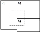
Figure 1:  An inconsistent spatial database

Suppose that a query requests all land parcels whose geometries intersect with a query window, which represents the spatial region shown in Figure 1 as a rectangle with dashed borders. Although the database instance is inconsistent, we can still obtain useful and meaningful answers. In this case, only the intersection of $g_{2}$ and $g_{3}$ is in conflict, but the rest of both geometries can be considered consistent and should be part of any “database repair” if we decide to restore consistency by means of minimal geometric changes. Thus, since the non-conflicting parts of geometries $g_{2}$ and $g_{3}$ intersect the query window, we would expect an answer including land parcels with identities ${\it idl_{1},idl_{2}}$ and ${\it idl_{3}}$. $\Box$

If we just concentrate on (in)consistency issues in databases (leaving aside consistent query answering for a moment), we can see that, in contrast to (in)consistency handling in relational databases, that has been largely investigated, not much research of this kind has been done for spatial databases. In particular, there is not much work around the formalization of semantic spatial ICs, satisfaction of ICs, and checking and maintenance of ICs in the spatial domain. However, some papers address the specification of some kinds of integrity constraints [8, 20], and checking topological consistency at multiple representations and for data integration [13, 14, 31].

More recently, [12] proposes qualitative reasoning with description logic to describe consistency between geographic data sets. In [22] a set of abstract relations between entity classes is defined; and they could be used to discover redundancies and conflicts in sets of SICs. A proposal for fixing (changing) spatial database instances under different types of spatial inconsistencies is given in [29]. According to it, changes are applied over geometries in isolation; that is, they are not analyzed in combination with multiple SICs. In [27] some issues around query answering under violations of functional dependencies involving geometric attributes were raised. However, the problem of dealing with an inconsistent spatial database, while still obtaining meaningful answers, has not been systematically studied so far.

Consistent query answering (CQA) from inconsistent databases as a strategy of inconsistent tolerance has an extensive literature (cf. [4, 6, 10] for surveys). It was introduced and studied in the context of relational database in [2]. They defined consistent answers to queries as those that are invariant under all the minimal forms of restoring consistency of the original database. Thus, the notion of repair of an instance with respect to a set of ICs becomes a fundamental concept for defining consistent query answers. A repair semantics defines the admissible and consistent alternative instances to an inconsistent database at hand. More precisely, a repair of an inconsistent relational instance ${\it D}$ is a consistent instance ${\it D}^{\prime}$ obtained from ${\it D}$ by deleting or inserting whole tuples. The set of tuples by which ${\it D}$ and ${\it D}^{\prime}$ differ is minimal under set inclusion [2]. Other types of repair semantics have been studied in the relational case. For example, in [16, 32] repairs are obtained by allowing updates of attribute values in tuples.

In comparison to the relational case, spatial databases offer new alternatives and challenges when defining a repair semantics. This is due, in particular, to the use of complex attributes to represent geometries, their combination with thematic attributes, and the nature of spatial (topological) relations.

In this work we define a repair semantics for spatial databases with respect to a subset of spatial semantic integrity constraints (a.k.a. topo-semantic integrity constraints) [29], which impose semantic restrictions on topological predicates and combinations thereof. In particular, we treat spatial semantic integrity constraints that can be expressed by denials constraints. For example, they can specify that “two land parcels cannot internally intersect”. This class of constraints are neither standardized nor integrated into current spatial database management systems (DBMSs); they rather depend on the application, and must be defined and handled by the database developers. They are very important because they capture the semantics of the intended models. Spatial semantic integrity constraints will be simply called spatial integrity constraints (SICs). Other spatial integrity constraints [11] are domain (topological or geometric) constraints, and they refer to the geometry, topology, and spatial relations of the spatial data types. One of them could specify that “polygons must be closed”. Many of these geometric constraints are now commonly integrated into spatial DBMSs [23].

A definition of a repair semantics for spatial DBs and CQA for spatial range queries was first proposed in [28], where we discussed the idea of shrinking geometries to solve conflicting tuples and applied to CQA for range queries. In this paper we complement and extend our previous work with the following main contributions: (1) We formalize the repair semantics of a spatial database instance under violations of SICs. This is done through virtual changes of geometries that participate in violations of SICs. Unlike [28], we identify the admissible local transformations and we use them to provide an inductive definition of database repair. (2) Based on this formalization, a consistent answer to a spatial query is defined as an answer obtained from all the admissible repairs. Extending the results in [28], we now define CQA not only for range but also for spatial join queries. (3) Although the repair semantics and consistent query answers can be defined for a fairly broad class of SICs and queries, as it becomes clear soon, naive algorithms for computing consistent answers on the basis of the computation of all repairs are of exponential time. For this reason, CQA for a relevant subset of SICs and range and join queries is done via a core computation. This amounts to querying directly the intersection of all repairs of an inconsistent database instance, but without actually computing the repairs. We show cases where this core can be specified as a view of the original, inconsistent database. (4)  We present an experimental evaluation with real and synthetic data sets that compares the cost of CQA with the cost of evaluating queries directly over the inconsistent database (i.e., ignoring inconsistencies).

The rest of the paper is organized as follows. In Section 2 we describe the spatial data model upon which we define the repair semantics and consistent query answers. A formal definition of repair for spatial inconsistent databases under SICs is introduced in Section 3. In Section 4 we define consistent answers to conjunctive queries. We analyze in particular the cases of range and join queries with respect to their computational properties. This leads us, in Section 5, to propose polynomial time algorithms (in data complexity) for consistent query answering with respect to a relevant class of SICs and queries. An experimental evaluation of the cost of CQA is provided in Section 6. Final conclusions and future research directions are given in Section 7.

2 Preliminaries

Current models of spatial database are typically seen as extensions of the relational data model (known as extended-relational or object-relational models) with the definition of abstract data types to specify spatial attributes. We now introduce a general spatio-relational database model that includes spatio-relational predicates (they could also be purely relational) and spatial ICs. It uses some of the definitions introduced in [25]. The model is independent of the geometric data model (e.g. Spaghetti [30], topological [18, 30], raster [19], or polynomial model [24]) underlying the representation of spatial data types.

A spatio-relational database schema is of the form $\Sigma=({\cal U},{\cal A},{\cal R},$ ${\cal T},{\cal O},{\cal B})$, where: (a) ${\cal U}$ is the possibly infinite database domain of atomic thematic values. (b) ${\cal A}$ is a set of thematic, non-spatial, attributes. (c) ${\cal R}$ is a finite set of spatio-relational predicates whose attributes belong to ${\cal A}$ or are spatial attributes. Spatial attributes take admissible values in ${\cal P}(\mathbb{R}^{m})$, the power set of $\mathbb{R}^{m}$, for an $m$ that depends on the dimension of the spatial attribute. (d) ${\cal T}$ is a fixed set of binary spatial predicates, with a built-in interpretation. (e) ${\cal O}$ is a fixed set of geometric operators that take spatial arguments, also with a built-in interpretation. (f) ${\cal B}$ is a fixed set of built-in relational predicates, like comparison predicates, e.g. $<,>,=,\neq$, which apply to thematic attribute values.

Each database predicate $R\in{\cal R}$ has a type $\tau(R)=[n,m]$, with $n,m\in\mathbb{N}$, indicating the number $n$ of thematic attributes, and the spatial dimension $m$ of the single spatial attribute (it takes values in ${\cal P}(\mathbb{R}^{m}$)). In Example 1, $\tau({\it LandP})=[1,2]$, since it has one thematic attribute (${\it idl}$) and one spatial attribute (${\it geometry}$) defined by a 2D polygon. In this work we assume that each relation $R$ has a key of the form (1) formed by thematic attributes only:

$$\forall\bar{x}_{1}\bar{x}_{2}\bar{x}_{3}s_{1}s_{2}~{}(R(\bar{x}_{1},\bar{x}_{2};s_{1})\wedge R(\bar{x}_{1},\bar{x}_{3};s_{2})\rightarrow(\bar{x}_{2}=\bar{x}_{3}\wedge s_{1}=s_{2})),$$ (1)

where the $\bar{x}_{i}$ are sequences of distinct variables representing thematic attributes of $R$, and the $s_{i}$ are variables for geometric attributes. Here $s_{1}=s_{2}$ means geometric equality; that is, the identity of two geometries.

A database instance ${\it D}$ of a spatio-relational schema $\Sigma$ is a finite collection of ground atoms (or spatial database tuples) of the form $R(c_{1},...,c_{n};s)$, where $R\in{\cal R}$, $\langle c_{1},...,c_{n}\rangle\in{\cal U}^{n}$ contains the thematic attribute values, and ${\it s}\in{\it Ad}\subseteq{\cal P}({\mathbb{R}}^{m})$, where ${\it Ad}$ is the class of admissible geometries (cf. below). The extension in a particular instance of a spatio-relational predicate is a subset of ${\cal U}^{n}\times{\it Ad}$. For simplicity, and to fix ideas, we will consider the case where $m=2$.

Among the different abstraction mechanisms for modelling single spatial objects, we concentrate on regions for modelling real objects that have an extent. They are useful in a broad class of applications in Geographic Information Systems (GISs). More specifically, our model will be compatible with the specification of spatial operators (i.e., spatial relations or geometric operations) as found in current spatial DBMSs [23]. Following current implementations of DBMSs, regions could be defined as finite sets of polygons that, in their turn, are defined through their vertices. This would make regions finitely representable. However, in this work geometries will be treated at a more abstract level, which is independent of the spatial model used for geometric representation. In consequence, an admissible geometry of the Euclidean plane is either the empty geometry, $g_{\oslash}$, which corresponds to the empty subset of the plane, or is a closed and bounded region with a positive area. It holds $g_{\oslash}\cap g=g\cap g_{\oslash}=g_{\oslash}$, for every region $g$. From now on, empty geometries and regions of $\mathbb{R}^{2}$ are called admissible geometries and they form the class ${\it Ad}$.

Geometric attributes are complex data types, and their manipulation may have an important effect on the computational cost of certain algorithms and algorithmic problems. As usual, we are interested in data complexity, i.e., in terms of the size of the database. The size of a spatio-relational database can be defined as a function of the number of tuples and the representation size of geometries in those tuples.

We concentrate on binary (i.e., two-ary) spatial predicates that represent topological relations between regions. They have a fixed semantics, and become the elements of ${\cal T}$. There are eight basic binary relations over regions of $\mathbb{R}^{2}$: ${\it Overlaps~{}(OV)}$, ${\it Equals~{}(EQ)}$, ${\it CoveredBy~{}(CB)}$, ${\it Inside~{}(IS)}$, ${\it Covers}$ ${\it(CV)}$, ${\it Includes~{}(IC)}$, ${\it Touches~{}(TO)}$, and ${\it Disjoint~{}(DJ)}$ [15, 26]. The semantics of the topological relations follows the point-set topology defined in [15], which is not defined for empty geometries. We will apply this semantics to our non-empty admissible geometries. For the case of the empty set, a separate definition will be given below. According to [15], an atom $T(x,y)$ becomes true if four conditions are simultaneously true. Those conditions are expressed in terms of emptyness ($\emptyset$) and non-emptyness ($\neg\emptyset$) of the intersection of their boundaries ($\delta$) and interiors ($\circ$). The definitions can be found in Table 1. For example, for non-empty regions $x,y$, ${\it TO}(x,y)$ is true iff all of $\delta(x)\cap\delta(y)\neq\emptyset$, $\circ(x)\cap\circ(y)=\emptyset$, $\delta(x)\cap\circ(y)=\emptyset$, and $\circ(x)\cap\delta(y)=\emptyset$ simultaneously hold.

Relation	$\delta(x)\cap\delta(y)$	$\circ(x)\cap\circ(y)$	$\delta(x)\cap\circ(y)$	$\circ(x)\cap\delta(y)$
DJ(x,y)	$\emptyset$	$\emptyset$	$\emptyset$	$\emptyset$
TO(x,y)	$\neg\emptyset$	$\emptyset$	$\emptyset$	$\emptyset$
EQ(x,y)	$\neg\emptyset$	$\neg\emptyset$	$\emptyset$	$\emptyset$
IS(x,y)	$\emptyset$	$\neg\emptyset$	$\neg\emptyset$	$\emptyset$
CB(x,y)	$\neg\emptyset$	$\neg\emptyset$	$\neg\emptyset$	$\emptyset$
IC(x,y)	$\emptyset$	$\neg\emptyset$	$\emptyset$	$\neg\emptyset$
CV(x,y)	$\neg\emptyset$	$\neg\emptyset$	$\emptyset$	$\neg\emptyset$
OV(x,y)	$\neg\emptyset$	$\neg\emptyset$	$\neg\emptyset$	$\neg\emptyset$

Table 1: Definition of topological relations between regions based on point-set topology

In this work we exclude the topological relation ${{\it D}isjoint}$ from ${\cal T}$. This decision is discussed in Section 3, where we introduce the repair semantics. In addition to the basic topological relations, we consider three derived relations that exist in current SQL languages and can be logically defined in terms of the other basic predicates: ${\it Intersects~{}(IT)}$, ${\it Within~{}(WI)}$, and ${\it Contains~{}(CO)}$. We also introduce a forth relation, IIntersects (II), that holds when the interiors of two geometries intersect. It can be logically defined as the disjunction of ${\it Overlaps}$, ${\it Within}$ and ${\it Contains}$ (cf. Figure 2). For all the topological relations in ${\cal T}$, their converse (inverse) relation is within the set. Some of them are symmetric, like ${\it Equals}$, ${\it Touches}$, and ${\it Overlaps}$. For the non-symmetric relations, the converse relation of ${\it CoveredBy}$ is ${\it Covers}$, of ${\it Inside}$ is ${\it Includes}$, and of ${\it Within}$ is ${\it Contains}$.

As mentioned before, the formal definitions of the topological relations [15, 26] do not consider the empty geometry as an argument. Indeed, at the best of our knowledge, no clear semantics for topological predicates with empty geometries exists. However, in our case we extent the definitions in order to deal with this case. This will allow us to use a classical bi-valued logic, where atoms are always true or false, but never undefined. According to our extended definition, for any $T\in{\cal T}$, $T(g_{1},g_{2})$ is false if $g_{1}=g_{\oslash}$ or $g_{2}=g_{\oslash}$. In particular, ${\it IS}(g,g_{\oslash})$ is false, for every admissible region $g$. In order to make comparisons with the empty region, we will introduce and use a special predicate ${\it IsEmpty}(\cdot)$ on admissible geometries, such that ${\it IsEmpty}(s)$ is true iff $s=g_{\oslash}$.

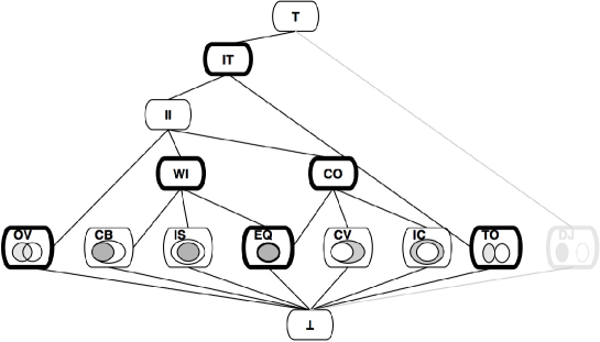
Figure 2:  Subsumption lattice of topological relations between regions: OV (Overlaps), CB (CoveredBy), IS (Inside), EQ (Equals), CV (Covers), IC (Includes), TO (Touches), DJ (Disjoint), IT (Intersects), II (IIntersects), WI (Within), and CO (Contains).

Notice that the semantics of the topological predicates, even for non-empty regions, may differ from the intuitive set-theoretic semantics one could assign to them. For example, for an admissible and non-empty geometry $g$, ${\it OV}(g,g)$ is false (due to the conditions in the last two columns in Table 1). In consequence, the constraint $\forall x\forall s^{\neq g_{\oslash}}\neg(R(x;s)\wedge{\it OV}(s,s))$ is satisfied.

Given a database instance, additional spatial information is usually computed from the explicit geometric data by means of the spatial operators in ${\cal O}$ associated with $\Sigma$. Some relevant operators are: ${\it Area}$, ${\it Union}$ (binary), ${\it Intersection}$, ${\it Difference}$, ${\it Buffer}$, and ${\it Union}$ ${\it Aggregation}$ ${\it(GeomUnion)}$. (Cf. [23] for the complete set of spatial predicates defined within the Open GIS Consortium.) There are several spatial operators used in this work; however, we will identify a particular subset ${\cal O}^{a}$ of spatial operators in ${\cal O}$, i.e., ${\cal O}^{a}\subseteq{\cal O}$, which will be defined for all admissible geometries and used to shrink geometries with the purpose of restoring consistency, as we describe in Section 3.

Definition 1

The set ${\cal O}^{a}$ of admissible operations contains the following geometric operations on admissible geometries $g$ and $g^{\prime}$:
      (1) ${\it Difference}(g,g^{\prime})$ is the topological closure of the set-difference.

(2) ${\it Buffer}(g,d)$ is the geometry obtained by buffering a distance $d$ around $g$, where $d$ is a distance unit. ${\it Buffer}(g,d)$ returns a closed region $\bar{g}$ containing geometry $g$, such that every point in the boundary of $\bar{g}$ is at a distance $d$ from some point of the boundary of $g$. In particular, ${\it Buffer}(g_{\oslash},d)=g_{\oslash}$.  $\Box$

Notice that these operators, when applied to admissible geometries, produce admissible geometries.

Remark 1

The value of $d$ in Definition 1 is instance dependent. It should be precomputed from the spatial input data. For this work, we consider $d$ to be a fixed value associated with the minimum distance between geometries in the cartographic scale of the database instance. $\Box$

A schema $\Sigma$ determines a many-sorted, first-order (FO) language ${\cal L}(\Sigma)$ of predicate logic. It can be used to syntactically characterize and express SICs. For simplicity, we concentrate on denial SICs, which are sentences of the form:

$$\forall^{\neq g_{\emptyset}}\bar{s}\forall\bar{x}~{}\neg(\bigwedge_{i=1}^{m}R_{i}(\bar{x}_{i};s_{i})\wedge\varphi\wedge~{}\bigwedge_{j=1}^{n}T_{j}(v_{j},w_{j})).$$ (2)

Here, $\bar{s}=s_{1}\cdots s_{m},~{}\bar{x}=\bar{x}_{1}\cdots\bar{x}_{m}$ are finite sequences of geometric and thematic variables, respectively, and $0<m,n\in\mathbb{N}$. Thus, each $\bar{x}_{i}$ is a finite tuple of thematic variables and will be treated as a set of attributes, such that $\bar{x}_{i}\subseteq\bar{x}_{j}$ means that the variables in $\bar{x}_{i}$ area also variables in $\bar{x}_{j}$. Also, $\forall\bar{x}$ stands for $\forall x_{1}\cdots\forall x_{m}$; and $\forall^{\neq g_{\emptyset}}\bar{s}$ stands for $\forall s_{1}\cdots\forall s_{m}$, with the universal quantifiers ranging over all the non-empty admissible geometries (i.e. regions). Here, $v_{j},w_{j}\in\bar{s}$, $R_{1},\ldots,R_{m}\in{\cal R}$, $\varphi$ is a formula containing built-in atoms over thematic attributes, and $T_{j}\in{\cal T}$. A constraint of the form (2) prohibits certain combinations of database atoms. Since topological predicates for empty geometries are always false, the restricted quantification over non-empty geometries in the constraints could be eliminated. However, we do not want to make the satisfaction of the constraints rely on our particular definition of the topological predicates for the empty region. In this way, our framework becomes more general, robust and modular, in the sense that it would be possible to redefine the topological predicates for the empty region without affecting our approach and results.

Example 2

Figure 3 shows an instance for the schema ${\cal R}=\{{\it LandP(idl,}$ ${\it name},$ ${\it owner};$ ${\it geometry)}$, ${\it Building(idb;}$ ${\it geometry)}\}$. Dark rectangles represent buildings and white rectangles represents land parcels. In ${\it LandP}$, the thematic attributes are ${\it idl,name}$ and ${\it owner}$, whereas ${\it geometry}$ is the spatial attribute of dimension $2$. Similarly for ${\it Building}$, which has only ${\it idl}$ as a thematic attribute.

The following sentences are denial SICs:  (The symbol $\bar{\forall}$ stands for the universal closure of the formula that follows it.)

$$\overline{\forall}\neg({\it LandP}(idl_{1},n_{1},o_{1};s_{1})\wedge{\it LandP}(idl_{2},n_{2},o_{2};s_{2})~{}\wedge idl_{1}\neq idl_{2}\wedge{\it IIntersects}(s_{1},s_{2})).$$ (3)

$${\footnotesize\overline{\forall}\neg({\it Building}(idb;s_{1})~{}\wedge~{}{\it LandP}(idl,n,o;s_{2})~{}\wedge{\it Overlaps}(s_{1},s_{2})).}$$ (4)

The SIC (3) says that geometries of land parcels with different ids cannot internally intersect (i.e., they can only be disjoint or touch). The SIC (4) establishes that building blocks cannot (partially) overlap land parcels. $\Box$

LandP
idl	name	owner	geometry
$idl_{1}$	$n_{1}$	$o_{1}$	$g_{1}$
$idl_{2}$	$n_{2}$	$o_{2}$	$g_{2}$
$idl_{3}$	$n_{3}$	$o_{3}$	$g_{3}$

Building
idb	geometry
$idb_{1}$	$g_{4}$
$idb_{2}$	$g_{5}$

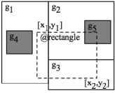
Figure 3:  A spatial database instance

A database instance ${\it D}$ for schema $\Sigma$ can be seen as an interpretation structure for the language ${\cal L}(\Sigma)$. For a set $\Psi$ of SICs in ${\cal L}(\Sigma)$,  ${\it D}\models\Psi$ denotes that each of the constraints in $\Psi$ is true in (or satisfied by) ${\it D}$. In this case, we say that ${\it D}$ is consistent with respect to $\Psi$. Correspondingly, ${\it D}$ is inconsistent with respect to $\Psi$, denoted ${\it D}\not\models\Psi$, when there is a $\psi\in\Psi$ that is violated by ${\it D}$, i.e., not satisfied by ${\it D}$. The instance in Example 2 is consistent with respect to its SICs.

In what follows, we will assume that the set $\Psi$ of SICs under consideration is logically consistent; i.e., that there exists a non-empty database instance ${\it D}$ (not necessarily the one at hand), such that ${\it D}\models\Psi$. For example, any set of SICs containing a constraint of the form $\forall^{\neq g_{\emptyset}}s\forall\bar{x}~{}\neg(R(\bar{x};s)\wedge{{\it E}quals}(s,s))$ is logically inconsistent. The analysis of whether a set of SICs is logically consistent or not is out of the scope of this work.

3 A Repair Semantics

Different alternatives for update-based consistency restoration of spatial databases are discussed in [28]. One of the key criteria to decide about the update to apply is minimality of geometric changes. Another important criteria may be the semantics of spatial objects, which makes changes over the geometry of one type of object more appropriate than others. For this work, the repair semantics is a rule applied automatically. It assumes that no previous knowledge about the quality and relevance of geometries exists and, therefore, it assumes that geometries are all equally important.

On the basis on the minimality condition on geometric changes and the monotonicity property of some topological predicates [28], we propose to solve inconsistencies with respect to SICs of the form (2) through shrinking of geometries. Notice that this repair semantics will be used as an instrumental concept to formalize consistent query answers (no actual modification over the database occurs). As such, it defines what part of the geometry is not in conflict with respect to a set of integrity constraints and can, therefore, be part of a consistent answer.

Shrinking geometries eliminates conflicting parts of geometries without adding new uncertain geometries by enlargement. In this way, we are considering a proper subset of the possible changes to fix spatial databases proposed in [29]. We disregard translating objects, because they will carry potentially new conflicts; and also creating new objects (object splitting), because we would have to deal with null or unknown thematic attributes.

The SICs of the form (2) exclude the topological predicate Disjoint. The reason is that falsifying an atom ${\it DJ}(g_{1},g_{2})$ by shrinking geometries is not possible, unless we make one of them empty. However, doing so would heavily depend upon our definition of this topological predicate for empty regions. Since we opted for not making our approach and results depend on this particular definition, we prefer to exclude the Disjoint predicate from our considerations. The study of other repair semantics that sensibly includes the topological predicate ${\it Disjoint}$ will be left for future work.

Technically, a database ${\it D}$ violates a constraint $\forall\bar{x}_{1}\bar{x}_{2}\forall^{\neq g_{\oslash}}s_{1}s_{2}$ $\neg(R_{1}(\bar{x}_{1};$ $s_{1})\wedge R_{2}(\bar{x}_{2};s_{2})\wedge\varphi\wedge T(s_{1},s_{2}))$, with $T\in{\cal T}$, when there are data values $\bar{a}_{1},\bar{a}_{2},g_{1},g_{2}$, with $g_{1},g_{2}\neq g_{\oslash}$, for the variables in the constraint such that $(R_{1}(\bar{x}_{1};s_{1})$ $\wedge R_{2}(\bar{x}_{2};s_{2})\wedge\varphi\wedge T(s_{1},s_{2}))$ becomes true in the database under those values. This is denoted with ${\it D}\models(R_{1}(\bar{x}_{1};s_{1})\wedge R_{2}(\bar{x}_{2};s_{2})\wedge\varphi\wedge T(s_{1},s_{2}))$ $[\bar{a}_{1},\bar{a}_{2},g_{1},g_{2}]$. When this is the case, it is possible to restore consistency of ${\it D}$ by shrinking $g_{1}$ or $g_{2}$ such that $T(g_{1},g_{2})$ becomes false.

We can compare geometries, usually an original geometry and its shrunk version, by means of a distance function that refers to their areas. We assume that ${\it area}\in{\cal O}$ is an operator that computes the area of a geometry.

Definition 2

For regions $g_{1},g_{2}$,  $\delta(g_{1},g_{2})~{}=~{}{\it area}({\it Difference}(g_{1},g_{2})\cup{\it Difference}(g_{2},g_{1}))$. $\Box$

Since we will compare a region $g_{1}$ with a region $g_{2}$ obtained by shrinking $g_{1}$, it will hold $\delta(g_{1},g_{2})\geq 0$. Indeed, when comparing $g_{2}\subseteq g_{1}$, the distance function can be simplified by $\delta(g_{1},g_{2})={\it area}({\it Difference}(g_{1},g_{2}))$. We will assume that it is possible to compare geometries through the distance function by correlating their tuples, one by one. This requires a correspondence between instances.

Definition 3

Let ${\it D},{\it D}^{\prime}$ be database instances of schema $\Sigma$. ${\it D}^{\prime}$ is $({\it D},f_{{\it D}^{\prime}})$-indexed if $f_{{\it D}^{\prime}}$ is a bijective function from ${\it D}$ to ${\it D}^{\prime}$, such that, for all $c_{1},\ldots,c_{n},s$: $f_{{\it D}^{\prime}}(R(c_{1},\ldots,c_{n};s))=R(c_{1},\ldots,c_{n};s^{\prime})$, for some region $s^{\prime}$. $\Box$

In a $({\it D},f_{{\it D}^{\prime}})$-indexed instance ${\it D}^{\prime}$ we can compare tuples one by one with their counterparts in instance ${\it D}$. In particular, we can see how the geometric attribute values differ. In some cases there is an obvious function $f_{{\it D}^{\prime}}$, for example, when there is a key from a subset of $\mathcal{A}$ to the spatial attribute $S$, or when relations have a surrogate key for identification of tuples. In these cases we simply use the notion of ${\it D}$-indexed. When the context is clear, we also use $f$ instead of $f_{{\it D}^{\prime}}$.

Example 3

(example 2 cont.) Consider the relational schema ${\it LandP(idl,}$ ${\it name,}$ ${\it owner};\textit{geometry)}$. For the instance ${\it D}$ given in Example 2, the following instance ${\it D}^{\prime}$ is $({\it{\it D},f})$-indexed

LandP
idl	name	owner	geometry
$idl_{1}$	$n_{1}$	$o_{1}$	$g_{7}$
$idl_{2}$	$n_{2}$	$o_{2}$	$g_{8}$
$idl_{3}$	$n_{3}$	$o_{3}$	$g_{9}$

Here, $f({\it LandP}({\it idl}_{1},n_{1},a_{1};g_{1}))$ $=$ ${\it LandP}({\it idl}_{1},n_{1},$ $a_{1};g_{7})$, etc. $\Box$

When restoring consistency, it may be necessary to consider different combinations of tuples and SICs. Eventually, we should obtain a new instance, hopefully consistent, that we have to compare to the original instance in terms of their distance.

Definition 4

Let ${\it D},{\it D}^{\prime}$ be spatial database instances over the same schema $\Sigma$, with ${\it D}^{\prime}$ $({\it D},f)$-indexed. The distance $\Delta({\it D},{\it D}^{\prime})$  between ${\it D}$ and ${\it D}^{\prime}$  is the numerical  value $\Delta({\it D},$ ${\it D}^{\prime})=\Sigma_{\bar{t}\in{\it D}}\delta(\Pi_{S}(\bar{t}),$ $\Pi_{S}(f(\bar{t})))$, where $\Pi_{S}(\bar{t})$ is the projection of tuple $\bar{t}$ on its spatial attribute $S$. $\Box$

Now it is possible to define a “repair semantics”, which is independent of the geometric operators used to shrink geometries.

Definition 5

Let ${\it D}$ be a spatial database instance over schema $\Sigma$, $\Psi$ a set of SICs, such that ${\it D}\not\models\Psi$. (a) An s-repair of ${\it D}$ with respect to $\Psi$ is a database instance ${\it D}^{\prime}$ over $\Sigma$, such that: (i) ${\it D}^{\prime}\models\Psi$. (ii) ${\it D}^{\prime}$ is $({\it D},f)$-indexed. (iii) For every tuple $R(c_{1},\ldots,c_{n};g)\in{\it D}$, if $f(R(c_{1},$ $\ldots,c_{n};g))$ $=R(c_{1},\ldots,c_{n};g^{\prime})$, then $g^{\prime}\subseteq g$. (b) A minimal s-repair ${\it D}^{\prime}$ of ${\it D}$ is a repair of ${\it D}$ such that, for every repair ${\it D}^{\prime\prime}$ of ${\it D}$, it holds $\Delta({\it D},{\it D}^{\prime\prime})\geq\Delta({\it D},{\it D}^{\prime})$. $\Box$

Proposition 1

If ${\it D}$ is consistent with respect to $\Psi$, then ${\it D}$ is also its only minimal s-repair.

Proof:   For ${\it D}^{\prime}={\it D}$, it holds: (i) ${\it D}^{\prime}\models\Psi$, (ii) ${\it D}^{\prime}$ is $({\it D},f)$-indexed, (iii) for every tuple $R(c_{1},\ldots,c_{n};g)\in{\it D}$, if $f(R(c_{1},$ $\ldots,c_{n};g))$ $=R(c_{1},\ldots,c_{n};g^{\prime})$, then $g^{\prime}=g$. In this case, $\Delta({\it D},{\it D}^{\prime})=0$. Any other consistent instance ${\it D}^{\prime\prime}$ obtained by shrinking any of ${\it D}$’s geometries and still obtaining admissible geometries gives $\Delta({\it D},{\it D}^{\prime\prime})>0$. $\Box$

This is an “ideal and natural” repair semantics that defines a collection of semantic repairs. The definition is purely set-theoretic and topological in essence. It is worth exploring the properties of this semantics and its impact on properties of consistent query answers (as invariant under minimal s-repairs) and on logical reasoning about them. However, for a given database instance we may have a continuum and infinite number of s-repairs since between two points we have an infinite number of points, which we want to avoid for representational and computational reasons.

In this work we will consider an alternative repair semantics that is more operational in nature (cf. Definition 8), leaving the previous one for reference. This operational definition of repair makes it possible to deal with repairs in current spatial DBMSs and in terms of standard geometric operators (cf. Lemma 1). Under this definition, there will always be a finite number of repairs for a given instance. Consistency will be restored by applying a finite sequence of admissible transformation operations to conflicting geometries.

It is easy to see that each true relationship (atom) of the form $T(g_{1},g_{2})$, with $T\in{\cal T}$, can be falsified by applying an admissible transformation in ${\cal O}^{a}$ to $g_{1}$ or $g_{2}$. Actually, they can be falsified in a canonical way. These canonical falsification operations for the different topological atoms are presented in Table 2. They have the advantages of: (a) being defined in terms of the admissible operators, (b) capturing the repair process in terms of the elimination of conflicting parts of geometries, and (c) changing one of the geometries participating in a conflict.

x Pred. $T$	x A true atom $T(g_{1},g_{2})$ becomes a false atom $T(g^{\prime}_{1},g^{\prime}_{2})$ with
x ${\it OV}$	x 1.  If ${\it area}(g_{1}\cap g_{2})\leq{\it area}(g_{1}\smallsetminus g_{2})$:
	$~{}~{}~{}~{}g^{\prime}_{1}={\it Difference}(g_{1},g_{2})$, $g^{\prime}_{2}=g_{2}$.
	2.  If ${\it area}(g_{1}\cap g_{2})>{\it area}(g_{1}\smallsetminus g_{2})$:
	$~{}~{}~{}~{}g^{\prime}_{1}={\it Difference}(g_{1},{\it Difference}(g_{1},g_{2}))$, $g^{\prime}_{2}=g_{2}$.
	3. If ${\it area}(g_{1}\cap g_{2})\leq{\it area}(g_{2}\smallsetminus g_{1})$:
	$~{}~{}~{}~{}g^{\prime}_{2}={\it Difference}(g_{2},g_{1})$, $g^{\prime}_{1}=g_{1}$.
	4. If ${\it area}(g_{1}\cap g_{2})>{\it area}(g_{2}\smallsetminus g_{1})$:
	$~{}~{}~{}~{}g^{\prime}_{2}={\it Difference}(g_{2},{\it Difference}(g_{2},g_{1}))$, $g^{\prime}_{1}=g_{1}$.
x ${\it IS,CB}$	x 1. If ${\it area}(g_{1}\cap g_{2})\leq{\it area}(g_{2}\smallsetminus g_{1})$:
	$~{}~{}~{}~{}g^{\prime}_{2}={\it Difference}(g_{2},g_{1})$, $g^{\prime}_{1}=g_{1}$.
	2. If ${\it area}(g_{1}\cap g_{2})>{\it area}(g_{2}\smallsetminus g_{1})$:
	$~{}~{}~{}~{}g^{\prime}_{2}={\it Difference}(g_{2},{\it Difference}(g_{2},g_{1}))$, $g^{\prime}_{1}=g_{1}$.
	3. $g^{\prime}_{1}={\it Difference}(g_{1},g_{2})$, $g^{\prime}_{2}=g_{2}$.
x ${\it IC,CV}$	x 1.  If ${\it area}(g_{1}\cap g_{2})\leq{\it area}(g_{1}\smallsetminus g_{2})$:
	$~{}~{}~{}~{}g^{\prime}_{1}={\it Difference}(g_{1},g_{2})$, $g^{\prime}_{2}=g_{2}$.
	2.  If ${\it area}(g_{1}\cap g_{2})>{\it area}(g_{1}\smallsetminus g_{2})$:
	$~{}~{}~{}~{}g^{\prime}_{1}={\it Difference}(g_{1},{\it Difference}(g_{1},g_{2}))$, $g^{\prime}_{2}=g_{2}$.
	3. $g^{\prime}_{2}={\it Difference}(g_{2},g_{1})$, $g^{\prime}_{1}=g_{1}$.
x ${{\it I}I,WI,CO}$	x 1. $g^{\prime}_{1}={\it Difference}(g_{1},g_{2})$, $g^{\prime}_{2}=g_{2}$.
	2. $g^{\prime}_{2}={\it Difference}(g_{2},g_{1})$, $g^{\prime}_{1}=g_{1}$.
x ${{\it T}O,IT}$	x1. $g^{\prime}_{1}={\it Difference}(g_{1},{\it buffer}(g_{2},d))$, $g^{\prime}_{2}=g_{2}$.
	2. $g^{\prime}_{2}={\it Difference}(g_{2},{\it buffer}(g_{1},d))$, $g^{\prime}_{1}=g_{1}$.
	(See Remark 1 for definition of $d$)
x ${\it EQ}$	x 1. $g^{\prime}_{1}=g_{\oslash}$, $g^{\prime}_{2}=g_{2}$.
	2. $g^{\prime}_{2}=g_{\oslash}$, $g^{\prime}_{1}=g_{1}$.

Table 2: Admissible transformations

More specifically, in Table 2 we indicate, for each relation $T\in{\cal T}$, alternative operations that falsify a true atom of the form $T(g_{1},g_{2})$. Each of them makes changes on one of the geometries, leaving the other geometry unchanged. The list of canonical transformations in this table prescribes particular ways of applying the admissible operators of Definition 1. Later on, they will also become the admissible or legal ways of transforming geometries with the purpose of restoring consistency.

For example, Table 2 shows that for ${\it Overlaps}(OV)$, there are in principle four ways to make false an atom ${\it Overlaps}(g_{1},g_{2})$ that is true. These are the alternatives 1. to 4. in that entry, where alternatives 1. and 2. change geometry $g_{1}$; and alternatives 3. and 4. change geometry $g_{2}$. Only one of these alternatives that satisfies its condition is expected to be chosen to falsify the atom. A minimal way to change a geometry depends on the relative size between overlapping and non-overlapping areas: (i) when the overlapping area between $g_{1}$ and $g_{2}$ is smaller than or equal to their non-overlapping areas, a minimal change over geometry $g_{1}$ is ${\it Difference}(g_{1},g_{2})$, and over $g_{2}$ is ${\it Difference}(g_{2},g_{1})$ (cases 1. and 3. for $OV$ in Table 2). (ii) When the non-overlapping areas of $g_{1}$ or $g_{2}$ are smaller than the overlapping area, a minimal change over geometry $g_{1}$ is ${\it Difference}(g_{1},$ ${\it Difference}(g_{1},g_{2}))$, and over geometry $g_{2}$ is ${\it Difference}(g_{2},$ ${\it Difference}(g_{2},g_{1}))$ (cases 2. and 4. for $OV$ in Table 2).

For the case when ${{\it E}quals}(g_{1},g_{2})$ is true, the transformations in Table 2 make either geometry, $g_{1}$ or $g_{2}$ empty to falsify the atom. However, there are other alternatives that by shrinking geometries would achieve the same result, but also producing smaller changes in terms of the affected area. A natural candidate update consists in applying the transformation $g^{\prime}_{1}=\textit{Difference}(g_{1},\textit{Buffer}(\textit{Boundary}(g_{2}),d))$ (similarly and alternatively for $g_{2}$). In this case, we just take away from $g_{1}$ the part of the internal area of width $d$ surrounding the boundary of $g_{1}$, to make it different from $g_{2}$. We did not follow this alternative for practical reasons: having two geometries that are topologically equal could, in many cases, be the result of duplicate data, and one of them should be eliminated. Moreover, this alternative, in comparison with the officially adopted in this work, may create new conflicts with respect to other SICs. Avoiding them whenever possible will be used later, when designing a polynomial algorithm for CQA based on the core of an inconsistent database instance (see Section 5).

Table 2 shows that Touches and Intersects are predicates for which the eliminated area is not completely delimited by the real boundary of objects. Actually, we need to separate the touching boundaries. We do so by buffering a distance $d$ around one of the geometries and taking the overlapping part from the other one.

The following result is obtained directly from Table 2.

Lemma 1

For each topological predicate $T\in{\cal T}$ and true ground atom $T(g_{1},g_{2})$, there are geometries $g_{1}^{\prime},g_{2}^{\prime}$ obtained by means of the corresponding admissible transformation in Table 2, such that $T(g_{1}^{\prime},g_{2}^{\prime})$ becomes false. $\Box$

The following definition defines, for each geometric predicate $T$, a binary geometric operator $tr^{T}$ such that, if $T(g_{1},g_{2})$ is true, then $tr^{T}(g_{1},g_{2})$ returns a geometry $g_{1}^{\prime}$ such that $T(g_{1}^{\prime},g_{2})$ becomes false. The definition is based on the transformations that affect geometry $g_{1}$ in Table 2.

Definition 6

Let $T\in{\cal T}$ be a topological predicate. We define an admissible transformation operator ${\it tr}^{T}:{\it Ad}\times{\it Ad}\to{\it Ad}$ as follows:

• If $T(g_{1},g_{2})$ is false, then ${\it tr}^{T}(g_{1},g_{2}):=g_{1}$.

• If $T(g_{1},g_{2})$ is true, then:

  $$tr^{T}(g_{1},g_{2}) := \left\{\begin{array}[]{l}{\it Difference}(g_{1},g_{2})\textrm{ if }{\it area}(g_{1}\cap g_{2})\leq{\it area}(g_{1}\smallsetminus g_{2})\\ {\it Difference}(g_{1},{\it Difference}(g_{1},g_{2})),\textrm{ otherwise }\end{array}\right.$$

  $$\textrm{ for }T\in\{OV,IC,CV\};$$

  $$tr^{T}(g_{1},g_{2}) := {\it Difference}(g_{1},g_{2}),\textrm{ for }T\in\{IS,CB,II,WI,CO\};$$

  $$tr^{T}(g_{1},g_{2}) := {\it Difference}(g_{1},{\it Buffer}(g_{2},d))\textrm{ for }T\in\{TO,IT\};$$

  $$tr^{T}(g_{1},g_{2}) := g_{\oslash}\textrm{ for }T\in\{EQ\}.\hskip 241.84842pt\Box$$

It can be easily verified that the admissible operations ${\it tr}^{T}$, applied to admissible geometries, produce admissible geometries. They can be seen as macros defined in terms of the basic operations in Definition 1, and inspired by Table 2. The idea is that the operator $tr^{T}$ takes $(g_{1},g_{2})$, for which $T(g_{1},g_{2})$ is true, and makes the latter false by transforming $g_{1}$ into $g^{\prime}_{1}$, i.e., $T(g^{\prime}_{1},g_{2})$ becomes false.

Definition 6 can also be used to formalize the transformations on geometry $g_{2}$ indicated in Table 2. First, notice that for the converse predicate $T^{c}$ of predicate $T$ it holds: $T^{c}(g_{1},g_{2})$ true iff $T(g_{2},g_{1})$. Secondly, the converse of a transformation operator can be defined by  $({\it tr}^{T})^{c}:={\it tr}^{(T^{c})}$. In consequence, we can apply ${\it tr}^{T^{c}}$ to $(g_{2},g_{1})$, obtaining the desired transformation of geometry $g_{2}$. In this way, all the cases in Table 2 are covered. For example, if we want to make false a true atom ${\it Inside}(g_{1},g_{2})$, we can apply $tr^{IS}\!(g_{1},g_{2})$, but also $tr^{IC}\!(g_{2},g_{1})$.

Example 4

Table  3 illustrates the application of the admissible transformations to restore consistency of predicates $T\in\{{{\it O}verlaps},{{\it T}ouches}\}$. The dashed boundary is the result of applying Buffer$(g,d)$. $\Box$

$T(g_{1},g_{2})$	Original	$Tr^{T}(g_{1},g_{2})$	$Tr^{T}(g_{2},g_{1})$
${{\it O}V}$
${{\it T}O}$

Table 3: Examples of admissible transformations

We now define the notion of accessible instance that results from an original instance, after applying admissible transformation operations to geometries. The application of sequences of operators solves violations of SICs. Accordingly, the accessible instances are defined by induction.

Definition 7

Let ${\it D}$ be a database instance. ${\it D}^{\prime}$ is an accessible instance from ${\it D}$ (with respect to a finite set of SICs $\Psi$), if ${\it D}^{\prime}$ is obtained after applying, a finite number of times, the following inductive rules (any of them, when applicable):
(1).   ${\it D}^{\prime}={\it D}$.

(2).  There is an accessible instance ${\it D}_{0}$ from ${\it D}$, such that, for some $\psi\in\Psi$ with a topological predicate $T$, ${\it D}_{0}\not\models\psi$ through tuples $R_{1}(\bar{a}_{1};g_{1})$ and $R_{2}(\bar{a}_{2};g_{2})$ in ${\it D}_{0}$, for which $T(g_{1},g_{2})$ is true; and
         (a) ${\it D}^{\prime}={\it D}_{0}\smallsetminus\{R_{1}(\bar{a_{1}},g_{1})\}\cup\{R_{1}(\bar{a_{1}},{\it tr}^{\!T}\!(g_{1},g_{2}))\}$,  or
         (b) ${\it D}^{\prime}={\it D}_{0}\smallsetminus\{R_{2}(\bar{a_{2}},g_{2})\}\cup\{R_{2}(\bar{a_{2}},{\it tr}^{\!T^{c}}\!\!(g_{2},g_{1}))\}$. $\Box$

Example 5

Consider the database instance in Figure 4(a) that is inconsistent with respect to SIC (3). An accessible instance from this inconsistent database is in Figure 4(b), where only $g_{1}$ has changed. This can be expressed in the following way: $LandP(idl_{1},n_{1},o_{1};g_{1}^{\prime})=LandP(idl_{1},n_{1},o_{1};{\it tr}^{II}({\it tr}^{II}(g_{1},g_{2}),g_{3}))$. $\Box$

LandP
idl	name	owner	geometry
$idl_{1}$	$n_{1}$	$o_{1}$	$g_{1}$
$idl_{2}$	$n_{2}$	$o_{2}$	$g_{2}$
$idl_{3}$	$n_{3}$	$o_{3}$	$g_{3}$

(a)

LandP
idl	name	owner	geometry
$idl_{1}$	$n_{1}$	$o_{1}$	$g_{1}^{\prime}$
$idl_{2}$	$n_{2}$	$o_{2}$	$g_{2}$
$idl_{3}$	$n_{3}$	$o_{3}$	$g_{3}$

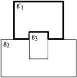
(b)

Figure 4: An accessible instance: (a) original instance, and (b) accessible transformation (geometry with thick boundary changed)

Given a database ${\it D}$, possibly inconsistent, we are interested in those accessible instances ${\it D}^{\prime}$ that are consistent, i.e., ${\it D}^{\prime}\models\Psi$. Even more, having the repairs in mind, we have to make sure that admissible instances from ${\it D}$ can still be indexed with ${\it D}$.

Proposition 2

Let ${\it D}^{\prime}$ be an accessible instance from ${\it D}$. Then, ${\it D}^{\prime}$ is $f$-indexed to ${\it D}$ via an index function $f$, that can be defined by induction on ${\it D}^{\prime}$.

Proof:   To simplify the presentation, we will assume that ${\it D}$ has an index (or surrogate key) $i_{0}$, that is a one-to-one mapping from ${\it D}$ to an initial segment $[1,N]$ of $\mathbb{N}$. Let ${\it D}^{\prime}$ be an accessible instance from ${\it D}$. We define $i_{{\it D}^{\prime}}(R(\bar{a};g))\in\mathbb{N}$ for tuples in ${\it D}^{\prime}$ by induction on ${\it D}^{\prime}$:
(1). If ${\it D}^{\prime}={\it D}$ and $R(\bar{a};g)\in{\it D}$, $i_{{\it D}^{\prime}}(R(\bar{a};g))=i_{0}(R(\bar{a};g))$.

(2). If there is an accessible instance ${\it D}_{0}$ from ${\it D}$ and ${\it D}_{0}\not\models\psi\in\Psi$ through the atoms $R_{1}(\bar{a}_{1};g_{1})$, $R_{2}(\bar{a}_{2};g_{2})$, and $T(g_{1},g_{2})$ with $T$ and $T^{c}$ the converse relation of $T$:
(a)  ${\it D}^{\prime}={\it D}_{0}\smallsetminus\{R_{1}(\bar{a}_{1},g_{1})\}\cup\{R_{1}(\bar{a}_{1},tr^{T}(g_{1},g_{2}))\}$, and $i_{{\it D}^{\prime}}(R_{1}(\bar{a}_{1};tr^{T}(g_{1},g_{2})))$ $=i_{{\it D}_{0}}(R_{1}(\bar{a}_{1},g_{1}))$ and $i_{{\it D}^{\prime}}(R_{2}(\bar{a}_{2};g_{2}))=i_{{\it D}_{0}}(R_{2}(\bar{a}_{2},g_{2}))$, or (b)  ${\it D}^{\prime}={\it D}_{0}\smallsetminus\{R_{2}(\bar{a}_{2},g_{2})\}\cup\{R_{2}(\bar{a}_{2},tr^{T^{c}}(g_{2},g_{1}))\}$, and $i_{{\it D}^{\prime}}(R_{1}(\bar{a}_{1};g_{1}))=i_{{\it D}_{0}}(R_{1}(\bar{a}_{1},g_{1}))$ and $i_{{\it D}^{\prime}}(R_{2}(\bar{a}_{2};tr^{T^{c}}(g_{2},g_{1})))=i_{{\it D}_{0}}(R_{2}(\bar{a}_{2},g_{2}))$. $\Box$

Any two accessible instances ${\it D}^{\prime}$ and ${\it D}^{\prime\prime}$ can be indexed via ${\it D}$ in a natural way, and thus, they can be compared tuple by tuple. In the following, we will assume, when comparing any two accessible instances in this way, that there is such an underlying index function $f$. Now we give the definition of operational repair.

Definition 8

Let ${\it D}$ be an instance over schema $\Sigma$ and $\Psi$ a finite set of SICs. (a) An o-repair of ${\it D}$ with respect to $\Psi$ is an instance ${\it D}^{\prime}$ that is accessible from ${\it D}$, such that ${\it D}^{\prime}\models\Psi$. (b) A minimal o-repair ${\it D}^{\prime}$ of ${\it D}$ is an o-repair of ${\it D}$ such that, for every o-repair ${\it D}^{\prime\prime}$ of ${\it D}$, $\Delta({\it D},{\it D}^{\prime\prime})\geq\Delta({\it D},{\it D}^{\prime})$. (c) ${\it Rep}({\it D},\Psi)$ denotes the set of minimal o-repairs of ${\it D}$ with respect to $\Psi$. $\Box$

The distances $\Delta({\it D},{\it D}^{\prime\prime})$ and $\Delta({\it D},{\it D}^{\prime})$ in this definition are relative to the corresponding index functions, whose existence is guaranteed by Proposition 2. Unless otherwise stated, this is the repair semantics we refer to in the remainder of the paper, in particular, in the definition of consistent query answer in Section 4. In consequence, in the following a repair is an o-repair, and the same applies to minimal repairs. Even more, whenever we refer to repairs, we should understand that minimal repairs are intended.

LandP
idl	name	owner	geometry
$idl_{1}$	$n_{1}$	$o_{1}$	$g_{1}$
$idl_{2}$	$n_{2}$	$o_{2}$	$g_{2}$
$idl_{3}$	$n_{3}$	$o_{3}$	$g_{3}$
$idl_{4}$	$n_{4}$	$o_{4}$	$g_{4}$

Building
idb	geometry
$idb_{1}$	$g_{5}$
$idb_{2}$	$g_{6}$

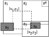
Figure 5: Inconsistent database instance

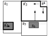
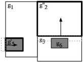
(a)		(b)

Figure 6: Minimal repairs

Example 6

Consider database schema in Example 2. The instance ${\it D}$ in Figure 5 is inconsistent with respect to the SICs (3) and (4), because the land parcels with geometries $g_{2}$ and $g_{3}$ overlap, and so do the land parcels with geometries $g_{2}$ and $g_{4}$. Likewise, buildings with geometry $g_{5}$ and $g_{6}$ partially overlap land parcels with geometries $g_{1}$ and $g_{2}$, respectively.

Figure 6 shows the two minimal repairs of ${\it D}$. In them, the regions with thicker boundaries are the regions that have their geometries changed. For the minimal repair in Figure 6(a), the inconsistency involving geometries $g_{2}$ and $g_{3}$ is repaired by applying ${\it Difference(g_{2},g_{3})}$ to $g_{2}$, i.e., removing from $g_{2}$ the whole overlapping geometry, and keeping the geometry of $g_{3}$ as originally. Notice that due to the interaction between integrity constraints, if we apply ${\it Difference(g_{3},g_{2})}$ to $g_{3}$, i.e., we remove the whole overlapping area from $g_{3}$, we still have an inconsistency, because the building with geometry $g_{6}$ will continue partially overlapping geometries $g_{2}$ and $g_{3}$. Thus, this change will require an additional transformation to ensure that $g_{6}$ is completely covered or inside of $g_{3}$.

In the same minimal repair (Figure 6(a)), the inconsistency between $g_{2}$ and $g_{4}$ is repaired by shrinking $g_{2}$, eliminating its area that overlaps $g_{4}$. This is obtained by applying ${\it Difference(g_{2},g_{4})}$ to $g_{2}$. Finally, the inconsistency between $g_{1}$ and $g_{5}$ is repaired by removing from $g_{5}$ its part that does not overlap with geometry $g_{1}$. In principle, we could have repaired this inconsistency by eliminating the overlapping region between $g_{1}$ and $g_{5}$, but this is not a minimal change.

In the second minimal repair (Figure 6(b)), geometries $g_{2}$ and $g_{5}$ undergo the same changes than those in the first minimal repair (Figure 6(a)), but the inconsistency between $g_{2}$ and $g_{4}$ is restored by eliminating geometry $g_{4}$, i.e., applying ${\it Difference}$ $(g_{4},g_{2})=g_{\oslash}$. $\Box$

Notice that, by applying admissible transformation operators to restore consistency, the whole part of a geometry that is in conflict with respect to another geometry is removed. In consequence, given that there are finitely many geometries in the database instance and finitely many SICs, a finite number of applications of admissible transformations are sufficient to restore consistency. This contrasts with the s-repair semantics, which can yield even a continuum of possible consistency-restoration transformations. Keeping the number of repairs finite may be crucial for certain mechanisms for computing consistent query answers, as those as we will show in the next sections. Actually, we will use existing geometric operators as implemented in spatial DBMSs in order to capture and compute the consistency-restoring geometric transformations. This will be eventually used to obtain consistent query answers for an interesting class of spatial queries and SICs in Section 5.2.

Despite the advantages of using o-repairs, the following example shows that an o-repair may not be minimal under the s-repair semantics.

Example 7

The instance ${\it D}$ in Figure 7 is inconsistent with respect to the SICs (3) and (4), because the land parcels with geometries $g_{1}$ and $g_{2}$ internally intersect and buildings with geometry $g_{3}$ and $g_{4}$ overlap land parcels with geometries $g_{1}$ and $g_{2}$, respectively.

Figures 8(a) and (b) show the minimal s-repair (Definition 5) and o-repairs of ${\it D}$ (Definition 8), respectively. In them, the regions with thicker boundaries are the regions that had their geometries changed. Here, by applying s-repair semantics we obtain one minimal repair (Figure 8(a)) that takes the partial conflicting parts from both land parcels $g_{1}$ and $g_{2}$ in conflict, and leave unchanged the geometries of buildings $g_{3}$ and $g_{4}$. Instead, for the o-repair semantics, each repair takes the whole conflicting parts from one of the land parcels $g_{1}$ or $g_{2}$ in order to satisfy SIC (3), and to satisfy SIC (4), each repair eliminates the conflict between the new version of $g_{1}$ and building $g_{3}$ or between the new version of $g_{2}$ and building $g_{4}$. This makes up to four possible o-repairs (Figure 8(b)), which are not minimal with respect to the single s-repair. $\Box$

LandP
idl	name	owner	geometry
$idl_{1}$	$n_{1}$	$o_{1}$	$g_{1}$
$idl_{2}$	$n_{2}$	$o_{2}$	$g_{2}$

Building
idb	geometry
$idb_{1}$	$g_{3}$
$idb_{2}$	$g_{4}$

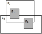
Figure 7: An inconsistent database instance

(a)		(b)

Figure 8: Minimal repairs: (a) minimal s-repair and (b) minimal o-repairs (thick boundaries show geometries that have changed)

S-repairs may take away only parts of a geometry that participate in a conflict. On the other side, they do not force a conflicting geometry to become empty in cases where o-repairs would do so. For instance, consider a true atom ${\it Equals}(g_{1},g_{2})$ that has to be falsified. A s-repair can be obtained by shrinking one of the two geometries just a little, without making it empty. However, by using admissible transformations, we can only falsify this atom by making one of the geometries empty. In this case, a minimal o-repair is not a minimal s-repair.

Proposition 3

Let ${\it D}$ be a database instance, and $\Psi$ a set of SICs. Then the following properties for o-repairs hold: (a) If ${\it D}$ is consistent with respect to $\Psi$, then ${\it D}$ is its only minimal o-repair. (b) If ${\it D}^{\prime}$ is an $({\it D},f)$-indexed o-repair of ${\it D}$ and $f(R(\bar{a};g))=R(\bar{a};g^{\prime})$, then $g^{\prime}\subseteq g$. (c) The set of o-repair for ${\it D}$ is finite and non-empty.

Proof:   (a) By the inductive definition of o-repair, an admissible transformation operator is applied to a geometry $g$ when $g$ is in conflict with other geometry $g^{\prime}$ in ${\it D}$. Since a consistent database instance does not contain conflicting tuples, none of the transformations operators is applicable and the consistent database instance is its only o-repair.
(b) The application of each admissible transformation ${\it tr}^{T}(g_{1},g_{2})$, with $T\in\cal{T}$, has five possible outcomes: $g_{1}$, $g_{\oslash}$, ${\it Difference}(g_{1},g_{2})$, ${\it Difference}(g_{1},{\it Difference}(g_{1},$ $g_{2}))$, or ${\it Difference}(g_{1},{\it Buffer}(g_{2},d))$. Then, by definition of operator ${\it Difference}$ (cf. Definition 1), ${\it tr}^{T}(g_{1},g_{2})\subseteq g_{1}$.
(c) ${\it D}$ has a finite number $N$ of tuples; and $\Psi$, a finite number of integrity constraints. In consequence, there is a finite number of conflicts, i.e., sets of tuples that simultaneously participate in the violation of one element $\psi$ of $\Psi$ via their geometries. Each of these conflicts are solved by shrinking some of those geometries. Each application of an operator $O$, chosen for a finite set of them, according to the inductive definition of o-repair solves an existing conflict by falsifying at least one of the $\mathcal{T}$-atoms in a ground instance of $\psi$. In principle, the application of such an operator $O$ may produce new conflicts; however, it strictly decreases the total geometrical area of the database instance. More precisely, if $A(D^{\prime}):=\Sigma_{R(\bar{t};g)\in D^{\prime}}{\it area}(g)$, then $A(D^{\prime})>A(O(D^{\prime}))$, where $O(D^{\prime})$ is the instance resulting from the conflict resolving operator $O$ to $D^{\prime}$. In particular, $A_{0}$ is the area $A(D)$ of the original instance $D$.

Now we reason by induction on the structure of o-repairs. The application of a one-conflict solving operator $O$ to an instance $D_{n-1}$ produces an instance $D_{n}$ with $A(D_{n})<A(D_{n-1})$. Moreover, $A(D_{n-1})-A(D_{n})>\epsilon>0$, where $\epsilon$ represents a lower bound of the area reduction at each inductive step.

We claim that, due to our repair semantics, this lower bound $\epsilon$ depends on the initial instance $D$, and not on $n$. In order to prove this, let us first remark that an admissible region is fully determined by its boundaries. Now we prove that the regions in any accessible instance depend on the regions in the original database instance, or, more precisely, by the boundaries delimiting those regions. We prove it by induction on the number of inductive steps of the definition of accessible instances.

First, we prove that it works for the first repair transformation on the original database instance. Let $g_{1}^{\prime}=Tr^{T}(g_{1},g_{2})$ be the first transformation applied on region $g_{1}$ to create the accessible instance ${\it D}_{1}$ from the original database instance ${\it D}$. For $T\in{\cal T}\setminus\{{\it TO,IT}\}$, and following the definitions of admissible transformations in Table 2, the geometry $g_{1}^{\prime}$ is either $g_{\oslash}$ or a region whose boundary is formed by parts of the boundaries that limit regions $g_{1}$ and $g_{2}$ (see example of overlapping regions in Figure 9). For $T\in\{{\it TO,IT}\}$, $g^{\prime}_{1}$ is formed by parts of the boundary of region $g_{1}$ and the boundary created by buffering $d$ around $g_{2}$. So, in this case, the boundary of $g_{1}^{\prime}$ depends exclusively on the boundaries of $g_{1}$ and $g_{2}$, and of the constant $d$.

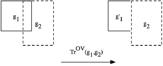
Figure 9: Example of a region’s boundary after geometric transformation

Let assume that the geometries in an accessible instance ${\it D}_{n}$ obtained after $n$ inductive steps are $g_{\oslash}$ or regions whose boundaries depend on the original instance. In the $n+1$ inductive step, another transformation $g_{i}^{\prime}=Tr^{T^{\prime}}(g_{i},g_{j})$ is applied. Following the definition of admissible transformations, $g_{i}^{\prime}$ becomes the geometry $g_{\oslash}$ or a region whose boundary is formed by part of the boundary of $g_{i}$ and part of the boundary of $g_{j}$, as in the first inductive step. Thus, $g_{i}^{\prime}$ also depends on the original database instance. This establishes our claim.

Now, by the Archimedean property of real numbers, there is a number $M$ such that $A_{0}-M\epsilon<0$. Thus, after a finite number of iterations (i.e. applications of conflict-solving operators), we reach a consistent instance or an instance with area $0$, i.e. all of whose geometries are empty, which would be consistent too.

Notice that the number $M$ provides an upper bound on the number of times we can apply operators to produce a repair. At each point we have a finite number of choices. So, the overall number of o-repairs that can be produced is finite. $\Box$

The following example shows that, even when applying admissible transformations, there may be exponentially many minimal repairs in the size of the database, a phenomenon already observed with relational repairs with respect to functional dependencies [6].

Example 8

Consider the schema in Example 2, and the SIC (3). The database instance contains $n$ spatial tuples, as shown in Figure 10. There are $n\!-\!1$ overlappings and $n$ overlapping geometries.

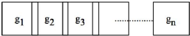
Figure 10: Exponential number of repairs

In order to solve each of those overlaps, we have the options of shrinking either one of the two regions involved. We have $2^{n-1}$ possible minimal repairs. $\Box$

The following remark is important when estimating the data complexity of repairs, because, in this case, data complexity does not only depend on the number of tuples, but also on the size of geometric representations.

Remark 2

Transformation operators that make geometries empty reduce the size of geometric representations. Any other admissible transformation operator ${\it tr}^{T}(g_{1},$ $g_{2})$ shrinks $g_{1}$, and uses $g_{1}$ and $g_{2}$ to define the new boundary of $g_{1}$. Thus, we are using, in a simple manner, the original geometric representation (e.g. points in the boundaries of the original geometries) to define a new geometry. It is clearly the case that there is a polynomial upper bound on the size of the representation of a new geometry in an o-repair in terms of the size of the original database, including representations of geometric regions. $\Box$

4 Consistent Query Answers

We can use the concept of minimal repairs as an auxiliary concept to define, and possibly compute, consistent answers to a relevant class of queries in ${\cal L}(\Sigma)$.

A general conjunctive query is of the form:

$${\cal Q}(\bar{v}):~{}\exists\bar{y}(R_{1}(\bar{x}_{1};s_{1})\wedge\cdots\wedge R_{n}(\bar{x}_{n};s_{n})\wedge\varphi),$$ (6)

where $\bar{v}=(\bigcup_{i}(\bar{x}_{i}\cup\{s_{i}\}))\smallsetminus\bar{y}$ are the free variables, and $\varphi$ is a conjunction of built-in atoms over thematic attributes or over spatial attributes that involve topological predicates in $\cal T$ and geometric operators in $\cal O$. We also add a safety condition, requiring that variables in $\varphi$ also appear in some of the $R_{i}$. For example, the following is a conjunctive query:

$${\cal Q}(x,y;s): \exists s_{1}s_{2}(R(x;s_{1})\wedge R(y;s_{2})\wedge{\it Intersects}(s_{1},s_{2})\wedge x\neq y\wedge s={\it Difference}(s_{1},s_{2})).$$

We will consider the simpler but common and relevant class of conjunctive queries that are operator free, i.e., conjunctive queries of the form (6) where $\varphi$ does not contain geometric operators. We will also study in more detail two particular classes of conjunctive queries:

• Spatial range queries are of the form

  $${\cal Q}(\bar{u};s):\exists\bar{z}(R(\bar{x};s)\wedge T(s,w)),$$ (7)

  with $w$ a spatial constant, and $\bar{z}\subseteq\bar{x}$. This is a “query window”, and its free variables are those in $\bar{u}=(\bar{x}\smallsetminus\bar{z})$ or in $\{s\}$.

• Spatial join queries are of the form

  $${\cal Q}(\bar{u};s_{1},s_{2}):\exists\bar{z}(R_{1}(\bar{x}_{1};s_{1})\wedge R_{2}(\bar{x}_{2};s_{2})\wedge T(s_{1},s_{2})),$$ (8)

  with $T\in\cal{T}$, and $\bar{z}\subseteq\bar{x}_{1}\cup\bar{x}_{2}$. The free variables are those in $\bar{u}=((\bar{x}_{1}\cup\bar{x}_{2})\smallsetminus\bar{z})$ or in $\{s_{1},s_{2}\}$.

We call basic conjunctive queries to queries of the form (7) or (8) with ${\it T}\in\{{\it IIntersects,Intersects}\}$.

Remark 3

Notice that for these two classes of queries we project on all the geometric attributes. We will also assume that the free variables correspond to a set of attributes of $R$ with its key of the form (1). More precisely, for range queries, the attributes associated with $\bar{u}$ contain the key of $R$. For join queries, $\bar{u}\cap\bar{x_{1}}$ and $\bar{u}\cap\bar{x_{2}}$ contain the key for relations $R_{1}$, $R_{2}$, respectively. This is a common situation in spatial databases, where a geometry is retrieved together with its key values. $\Box$

Given a query ${\cal Q}(\bar{x};\bar{s})$, with free thematic variables $\bar{x}$ and free geometric variables $\bar{s}$, a sequence of thematic/spatial constants $\langle\bar{c};\bar{g}\rangle$ is an answer to the query in instance ${\it D}$ if and only if ${\it D}\models{\cal Q}(\bar{c};\bar{g})$, that is the query $\cal Q$ becomes true in ${\it D}$ as a formula when its free variables $\bar{x},\bar{s}$ are replaced by the constants in $\bar{c},\bar{g}$, respectively. We denote with ${\cal Q}({\it D})$ the set of answers to ${\cal Q}$ in instance ${\it D}$.

Example 9

Figure 11 shows an instance for the schema ${\cal R}=\{{\it LandP(idl};$ ${\it geometry)}$, ${\it Building(idb;}$ ${\it geometry)}\}$. Here, ${\it idl,idb}$ are keys for their relations. Dark rectangles represent buildings, and white rectangles represent land parcels. The queries ${\cal Q}_{1}$ and ${\cal Q}_{2}$ below are a range and a join query, respectively. For the former, the spatial constant is the spatial window shown in Figure 11, namely the (closed) polygon obtained by joining the four points in order indicated in the query.

$${\cal Q}_{1}({{\it i}db;g}) : ~{}{\it Building}(idb;g)~{}\wedge$$

$${{\it I}ntersects(g},([x_{1},y_{1}],[x_{2},y_{1}],[x_{2},y_{2}],[x_{1},y_{2}],[x_{1},y_{1}])).$$

$${\cal Q}_{2}({{\it i}dl,idl^{\prime};g,g^{\prime}}) : ~{}{\it LandP}(idb;g)~{}\wedge~{}{\it LandP}(idb^{\prime};g^{\prime})~{}\wedge{{\it T}ouches}(g,g^{\prime}).$$

LandP
idl	geometry
${\it idl}_{1}$	$g_{1}$
${\it idl}_{2}$	$g_{2}$
${\it idl}_{3}$	$g_{3}$

Building
idb	geometry
${\it idb}_{1}$	$g_{4}$
${\it idb}_{2}$	$g_{5}$

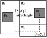
Figure 11:  Example of a range query

The answer to ${\cal Q}_{1}$ is $\langle{{\it i}db}_{2};g_{5}\rangle$. The answers to ${\cal Q}_{2}$ are: $\{\langle{{\it i}dl}_{1},{{\it i}dl}_{2};g_{1},g_{2}\rangle,$ $\langle{{\it i}dl}_{2},{{\it i}dl}_{3};g_{2},g_{3}\rangle,$  $\langle{{\it i}dl}_{1},{{\it i}dl}_{3};$ $g_{1},g_{3}\rangle$,  $\langle{{\it i}dl}_{2},{{\it i}dl}_{1};g_{2},g_{1}\rangle,$ $\langle{{\it i}dl}_{3},{{\it i}dl}_{2};g_{3},g_{2}\rangle,$ $\langle{{\it i}dl}_{3},{{\it i}dl}_{1};g_{3},g_{1}\rangle\}$. $\Box$

Now we define the notion of consistent answer to a conjunctive query.

Definition 9

Consider an instance ${\it D}$, a set $\Psi$ of SICs, and a conjunctive query ${\cal Q}(\bar{x};\bar{s})$. A tuple of thematic/geometric constants $\langle c_{1},\ldots$ $,c_{m};g_{1},\ldots,g_{l}\rangle$ is a consistent answer to ${\cal Q}$ with respect to $\Psi$ if:  (a) For every ${\it D}^{\prime}\in{\it Rep}({\it D},\Psi)$, there exist $g_{1}^{\prime},\ldots,g_{l}^{\prime}$ such that ${\it D}^{\prime}\models{\cal Q}(c_{1},\dots,c_{m};g_{1}^{\prime},\ldots,g_{l}^{\prime})$. (b) $g_{i}$ is the intersection over all regions $g_{i}^{\prime}$ that satisfy (a) and are correlated to the same tuple in ${\it D}$.  ${{\it C}on}({\cal Q},{\it D},\Psi)$ denotes the set of consistent answers to ${\cal Q}$ in instance ${\it D}$ with respect to $\Psi$. $\Box$

Since ${\cal Q}$ is operator free, the regions $g_{i}^{\prime}$ appear in relations of the repairs, and then $f^{-1}$ can be applied. However, due to the intersection of geometries, the geometries in a consistent answer may not belong to the original instance or to any of its repairs.

In contrast to the definition of consistent answer to a relational query [2], where a consistent answer is an answer in every repair, here we have an aggregation of query answers via the geometric intersection and grouped-by thematic tuples. This definition is similar in spirit to consistent answers to aggregate relational queries with group-by [3, 9, 17].

This definition of consistent answer allows us to obtain more significative answers than in the relational case, because when shrinking geometries, we cannot expect to have, for a fixed tuple of thematic attribute values, the same geometry in every repair. If we did not use the intersection of geometries, we might lose or not have consistent answers due to the lack of geometries in common among repairs.

idl geometry ${\it idl}_{1}$ $g_{1}$ ${\it idl}_{2}$ $g^{\prime}_{2}$ ${\it idl}_{3}$ $g_{3}$

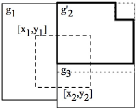
Figure 12:  Consistent answers

Example 10

(example 6 cont.) Consider the spatial range query
${\cal Q}({\it idl;geometry}):$  $\exists{\it name~{}owner}({\it LandP(idl,name,owner;geometry)}~{}\wedge$
                          ${\it Intersects(geometry},([x_{1},y_{1}],[x_{2},y_{1}],[x_{2},y_{2}],[x_{1},y_{2}],[x_{1},y_{1}])),$
which is expressed in the SQL language as:

SELECT $${\it idl,geometry}$$

FROM $${\it LandP}$$

WHERE $${\it Intersects}({\it geometry},([x_{1},y_{1}],[x_{2},y_{1}],[x_{2},y_{2}],[x_{1},y_{2}],[x_{1},y_{1}])).$$

Now, consider the two minimal repairs in Figure 6. In them, objects ${\it idl_{1}}$ and ${{\it i}dl}_{3}$ do not change geometries, whereas object ${\it idl_{2}}$ does, from $g_{2}$ to $g^{\prime}_{2},g_{2}^{\prime\prime}$, resp. (cf. Figure 6(a), (b), resp.).

From the first repair we get the following (usual) answers to the query: $\langle{\it idl}_{1};g_{1}\rangle$, $\langle{\it idl}_{2};g_{2}^{\prime}\rangle,\langle{\it idl}_{3};g_{3}\rangle$. From the second repair, we obtain $\langle{\it idl}_{1};g_{1}\rangle,\langle{\it idl}_{2};g_{2}^{\prime\prime}\rangle,\langle{\it idl}_{3};$ $g_{3}\rangle$. The consistent answers are the tuples shown in Figure 12, where the answers obtained in the repairs are grouped by an idl in common, and the associated geometries are intersected. In this figure, the geometry with thicker lines corresponds to the intersection of geometries obtained from different repairs.

From a practical point of view, the consistent query answer could include additional information about the degree in which geometries differ from their corresponding original geometries. For example, for the answer $\langle{\it idl}_{2};g_{2}^{\prime}\rangle$, an additional information could be the relative difference between areas $g_{2}$ and $g_{2}^{\prime}$, which is calculated by $\delta(g_{2},g_{2}^{\prime})/area(g_{2})$. $\Box$

5 Core-Based CQA

The definition of consistent query answer relies on the auxiliary notion of minimal repair. However, since we may have a large number of repairs, computing consistent answers by computing, materializing, and finally querying all the repairs must be avoided whenever there are more efficient mechanisms at hand. Along these lines, in this section we present a methodology for computing consistent query answers to a subclass of conjunctive queries with respect to certain kind of SICs. It works in polynomial time (in data complexity), and does not require the explicit computation of the database repairs.

We start by defining the ${\it core}$, which is a single database instance associated with the class of repairs. We will use the core to consistently answer a subclass of conjunctive queries. Intuitively, the core is the “geometric intersection” of the repairs, which is obtained by intersecting the geometries in the different repair instances that correlate to the same thematic tuple.

Definition 10

For an instance ${\it D}$ and a set $\Psi$ of SICs, the core of ${\it D}$ is the instance ${\it D}^{\star}$ given by  ${\it D}^{*}:=$ $\{R(\bar{a};g^{\star})~{}|~{}R\in{\cal R},\mbox{ there is }R(\bar{a};g)\in{\it D}\mbox{ and }g^{\star}=\bigcap\{g^{\prime}~{}|$ $R(\bar{a};g^{\prime})\in{\it D}^{\prime}~{}\mbox{ for some }~{}{\it D}^{\prime}\in{\it Rep}({\it D},\Psi)$  $\mbox{and }~{}R(\bar{a};g^{\prime})=f_{{\it D}^{\prime}}(R(\bar{a};g))\}\}$. Here, $f_{{\it D}^{\prime}}$ is the correlation function for ${\it D}^{\prime}$. $\Box$

Sometimes we will refer to ${\it D}^{\star}$ by $\bigcap^{g}{\it Rep}({\it D},\Psi)$. However, it cannot be understood as the set-theoretic intersection of the repairs of ${\it D}$. Rather it is a form of geometric intersection of geometries belonging to different repairs and grouped by common thematic attributes. It is important to remark that the keys of relations remain in the repairs, and therefore they appear in the core of a dimension instance.

Example 11

Figure 13 shows the core of the database instance in Figure 5 considering the repairs in Figure 6. Here, $g^{*}_{2}$ results from the geometric intersection of geometries $g_{2}^{\prime}$ and $g_{2}^{\prime\prime}$ of the minimal repairs in Figure 6. Similarly, $g^{*}_{5}$ is $g_{5}^{\prime}$, because the latter is shared by both minimal repairs in Figure 6. Geometry $g_{4}$ becomes $g_{\oslash}$ in the core. All other geometries in the core are unchanged with respect to geometries in the original database instance. $\Box$

LandP∗
$idl_{1}$	$n_{1}$	$o_{1}$	$g^{*}_{1}$
$idl_{2}$	$n_{2}$	$o_{2}$	$g^{*}_{2}$
$idl_{3}$	$n_{3}$	$o_{3}$	$g^{*}_{3}$
$idl_{4}$	$n_{4}$	$o_{4}$	$g_{\oslash}$

Building∗
$idb_{1}$	$g^{*}_{5}$
$idb_{2}$	$g^{*}_{6}$

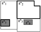
Figure 13:  The core of an instance

Notice the resemblance between the definitions of consistent answer and the core. Actually, it is easy to see that ${\it D}^{\star}=\bigcup_{\ R\in\cal{R}}{{\it C}on}({\cal Q}_{R},{\it D},\Psi)$, where the query ${\cal Q}_{R}(\bar{x};s):R(\bar{x};s)$ asks for the tuples in relation $R$.

The ${\it core}$ is defined as the geometric intersection of all database repairs. However, as we will show, for a subset of SICs we can actually determine the ${\it core}$ without computing these repairs. This is possible for SICs of the form:

$$\forall\bar{x}_{1}\bar{x}_{2}s_{1}s_{2}\neg(R(\bar{x}_{1};s_{1})~{}\wedge~{}R(\bar{x}_{2};s_{2})~{}\wedge~{}\bar{x}^{\prime}_{1}\neq\bar{x}^{\prime}_{2}\wedge~{}\it{T}(s_{1},s_{2})),$$ (9)

where ${\it T}\in\{{\it IIntersects,Intersects,Equals}\}$, $\bar{x}^{\prime}_{1}\subseteq\bar{x}_{1}$, $\bar{x}^{\prime}_{2}\subseteq\bar{x}_{2}$, and both $\bar{x}^{\prime}_{1}$ and $\bar{x}^{\prime}_{2}$ are the key of $R$. In these SICs there are two occurrences of the same database predicate in the same SIC. The following example illustrates this class of SICs.

Example 12

For the schema ${\cal R}=\{{\it County(idc,}$ ${\it name}$; ${\it geometry)}$, ${\it Lake(idl;}$ ${\it geometry)}\}$, with ${{\it i}dc}$ the key of ${{\it C}ounty}$ and ${{\it i}dl}$ the key of ${{\it L}ake}$, the following SICs are of the form (9):

$$\overline{\forall}\neg({\it County}(idc_{1},n_{1};s_{1})\wedge{\it County}(idc_{2},n_{2};s_{2})~{}\wedge idc_{1}\neq idc_{2}\wedge{\it IIntersects}(s_{1},s_{2})).$$ (10)

$$\overline{\forall}\neg({\it Lake}(idl_{1};s_{1})\wedge{\it Lake}(idl_{2};s_{2})~{}\wedge idl_{1}\neq idl_{2}\wedge{\it Intersects}(s_{1},s_{2})).$$ (11)

$\Box$

Remark 4

This subset of SICs has the following properties, which will be useful when trying to compute the repairs and the core:

• Two SICs of the form (9) over the same database predicate are redundant due to the semantic interrelation of the topological predicates IIntersects, Intersects, and Equals: only the constraint that contains the weakest topological predicate has to be considered. For example, Intersects is weaker than IIntersects, and IIntersects is weaker than Equals.

• Conflicts between tuples with respect to SICs of the form (9) are determined by the intersection of their geometries. The conflict between two tuples $R(\bar{a}_{1};g_{1})$ and $R(\bar{a}_{2};g_{2})$ is solved by applying a single admissible transformation operator $tr^{T}(g_{1},g_{2})$ (or $tr^{T^{c}}(g_{2},g_{1})$) that modifies $g_{1}$ (or $g_{2}$), and makes $T(g_{1},g_{2})$ (and $T^{c}(g_{2},g_{1})$) false.

• Solving conflicts with respect to a SIC of the form (9) is independent from solving a conflict with respect to another SIC of form (9) over a different database predicate.

• Solving a conflict between two tuples with respect to a SIC of the form (9) does not introduce new conflicts. This is due to the definition of admissible transformations and the monotonicity property of predicates IIntersects and Intersects, which prevent a shrunk geometry (or even an empty geometry) from participating in a new conflict with an existing geometry in the database (cf. Example 13).

• For any two geometries $g_{1}$ and $g_{2}$ in conflict with respect to a SIC of the form (9), there always exist two repairs, one with the shrunk version of $g_{1}$, and another with the shrunk version of $g_{2}$. This guarantees that there exists a minimal repair that contains a minimum version of a geometry whose its geometric intersections with original geometries in conflict have been eliminated (cf. Lemma 2). As a consequence, the core can be computed by taking from a geometry all its intersections with other geometries in conflict, disregarding the order in which these intersections are eliminated.

  This property is not guaranteed for other kinds of SICs. For instance, consider Example 6 with the instance in Figure 5 and its corresponding repairs in Figure 6. Although $g_{6}$ was originally in conflict with respect to $g_{2}$, there is no minimal repair where geometry $g_{6}$ is shrunk. $\Box$

We illustrate some of these properties with the following example.

County
idl	name	geometry
$idc_{1}$	$n_{1}$	$g_{1}$
$idc_{2}$	$n_{2}$	$g_{2}$
$idc_{3}$	$n_{3}$	$g_{3}$
$idc_{4}$	$n_{4}$	$g_{4}$
$idc_{4}$	$n_{5}$	$g_{5}$

Lake
idl	geometry
$idl_{1}$	$g_{6}$
$idl_{2}$	$g_{7}$

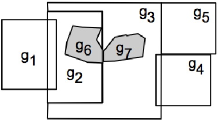
Figure 14:  An inconsistent database with SICs of the form (9)

Example 13

(example 12 cont.) Consider the inconsistent instance in Figure 14. In it, counties with geometries $g_{1}$, $g_{2}$ and $g_{3}$ are inconsistent with respect to SIC (10), because they internally intersect. Also, county $g_{3}$ internally intersects with geometry $g_{4}$. Lakes with geometries $g_{6}$ and $g_{7}$ violate SIC (11), because they intersect (actually they touch).

Conflicts with respect to SICs (10) and (11) can be solved in an independent way, since they do not share predicates (cf. Remark 4(iii)). To obtain a repair, consider first SIC (10) and the conflict between $g_{2}$ and $g_{3}$, which is solved by applying $tr^{{\it II}}(g_{2},g_{3})$ or $tr^{{\it II}}(g_{3},g_{2})$. Any of these alternative transformations do not produce geometries that could be in conflict with other geometries unless they were originally in conflict (cf. Remark 4(iv)). For instance, if we apply $tr^{{\it II}}(g_{3},g_{2})$ we obtain a new geometry $g^{\prime}_{3}$ that will be in conflict with geometries $g_{1}$ and $g_{4}$. These conflicts are not new, since $g_{3}$ was originally in conflict with these two geometries. Even more, by shrinking $g_{2}$ or $g_{3}$, none of the modified geometries could be in conflict with $g_{5}$. In addition, although by making $g^{\prime}_{3}=tr^{{\it II}}(g_{3},g_{2})$ we also solve the conflict between $g_{1}$ and $g_{3}$, this is only accomplished due to the fact the conflicting part of $g_{3}$ and $g_{1}$ has been already eliminated from $g^{\prime}_{3}$ (cf. Remark 4(v)).

Figure 15 shows the sixteen possible minimal repairs that are obtained by considering the eight possible ways in which conflicts with respect to SIC (10) are solved, in combination with the two possible ways in which conflicts with respect to SIC (11) are solved. In this figure thick boundaries represent geometries that have changed. Notice that in this figure we only show $g^{\prime}_{2_{1}}$ and not $g^{\prime}_{2_{2}}$, since the later corresponds to the empty geometry which is then omitted in the corresponding repairs. The core for this database instance is shown in Figure 16. $\Box$

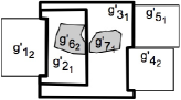
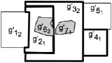
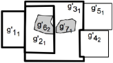
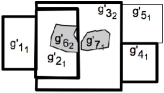
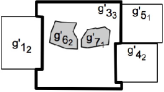
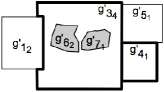
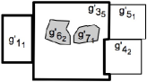
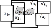
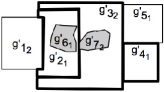
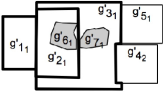
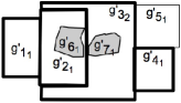
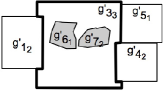
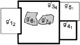
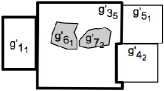
Figure 15: The sixteen possible repairs of Example 13

County∗
idl	name	geometry
$idc_{1}$	$n_{1}$	$g^{\prime}_{1_{1}}$
$idc_{2}$	$n_{2}$	$g_{\oslash}$
$idc_{3}$	$n_{3}$	$g^{\prime}_{3_{1}}$
$idc_{4}$	$n_{4}$	$g^{\prime}_{4_{1}}$
$idc_{4}$	$n_{5}$	$g^{\prime}_{5_{1}}$

Lake∗
idl	geometry
$idl_{1}$	$g^{\prime}_{6_{1}}$
$idl_{2}$	$g^{\prime}_{7_{1}}$

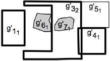
Figure 16: The core of Example 13

It is possible to use a tree to represent all the versions that a geometry $g$ may take in the repairs. The root of that tree is the original geometry $g$, the leaves are all the possible versions of the $g$ in the minimal repairs. The internal nodes represent partial transformations applied to $g$ as different conflicts in which $g$ participates are solved. For illustration, Figure 17 shows the tree that represents the possible different versions of $g_{3}$ in the minimal repairs for the inconsistent instance in Figure 14. Notice that a leaf in this tree represents a version of $g_{3}$ in a repair, which is not necessarily a minimum geometry. For instance, in Figure 17 the minimum version of $g_{3}$ is $g^{\prime}_{3_{1}}$. For all other non-minimum versions of $g_{3}$ in the leaves, conflicting areas are taken from other geometries. For example, geometry $g^{\prime}_{3_{6}}$ results by keeping $g_{3}$ as originally and shrinking geometries $g_{1}$, $g_{2}$ and $g_{4}$.

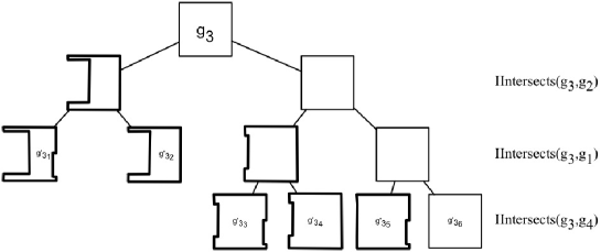
Figure 17: A tree-based representation of derived geometries from $g_{3}$ in some of the possible minimal repairs (thick boundaries represent geometries that have changed)

The following lemma establishes that when a geometry $g$ is involved in conflicts of SICs of the form (9), there exists a version of $g$ in the repairs that is minimum with respect to set-theoretic (geometric) inclusion. This result is useful to show that the minimum version of $g$ is the one that will be in the core.

We need to introduce the set ${\cal G}_{R,\Psi}(\bar{a},g)$ that contains, for a given tuple $R(\bar{a};g)$ in a database instance ${\it D}$, all the possible versions of geometry $g$ in the minimal repairs of ${\it D}$.

Definition 11

Let ${\it D}$ a database instance, a set $\Psi$ of SICs of the form (9) and a fixed tuple $R(\bar{a};g)\in{\it D}$. Then, ${\cal G}_{R,\Psi}(\bar{a},g)=\{g^{\prime}|R(\bar{a};g^{\prime})$ $\in{\it D}^{\prime},{\it D}^{\prime}\in{\it Rep}({\it D},\Psi)\},$ $f^{-1}(R(\bar{a};g^{\prime}))=R(\bar{a};g)$. $\Box$

Lemma 2

The set of geometries ${\cal G}_{R,\Psi}(\bar{a},g)$ has a minimum element $g_{min}$ under set-theoretic inclusion.

Proof:   By properties of SICs of the form (9), for each conflict in which $R(\bar{a};g)\in{\it D}$ participates, we can or cannot shrink $g$. This leads to a combination of possible transformations over geometry $g$ that can be represented in a binary tree as shown in Figure 17. So, we have a non-empty set of geometries ${\cal G}_{R,\Psi}(\bar{a},g)$.

In this tree, we always have a path from the root to a leaf in which the geometry is always shrunk; that is, all conflicting areas are eliminated from $g$. The leaf geometry in this path (repair) is the minimum geometry $g_{min}$. $\Box$

Corollary 1

Consider a database instance ${\it D}$, a set $\Psi$ of SICs of the form (9), and a fixed tuple $R(\bar{a};g)\in{\it D}$. For $g_{min}$, the minimum geometry in ${\cal G}_{R,\Psi}(\bar{a},g)$, it holds $R(\bar{a};g_{min})\in{\it D}^{\star}$.

Proof:   Direct from Lemma 2 and the definition of the core as a geometric intersection. $\Box$

5.1 Properties of the Core

In this section we establish that for the set of SICs of the form (9), and basic conjunctive queries, it is possible to compute consistent answers on the basis of the core of an inconsistent instance, avoiding the computation of queries in every minimal repair. This is established in Theorems 1 and 2, respectively.

Theorem 1

For an instance ${\it D}$, a set $\Psi$ of SICs of the form (9), and a basic spatial range query ${\cal Q}(\bar{u};s)$, it holds $\langle\bar{a};g\rangle\in{{\it C}on}({\cal Q},{\it D},\Psi)$ if and only if $\langle\bar{a};g\rangle\in{\cal Q}({\it D}^{*})$.

Proof:   The projection of range queries always includes the key of the relation in the result. Thus, if $\langle\bar{a},g\rangle\in{{\it C}on}({\cal Q},{\it D},\Psi)$, then for every ${\it D}^{\prime}\in{\it Rep}({\it D},\Psi)$, there exists $R(\bar{b};g^{\prime})$, such that $\bar{a}\subseteq\bar{b}$, $f^{-1}(R(\bar{b};g^{\prime}))=R(\bar{b};g)$ and $R(\bar{b};g)\in{\it D}$, where $T(g^{\prime},w)$ is true for the spatial constant $w$ of the range query and $g=\bigcap g^{\prime}$ with the intersection ranging over all $g^{\prime}$.

By Lemma 2, there exists tuple $R(\bar{b};g_{min})\in{\it D}^{\prime}\in{\it Rep}({\it D},\Psi)$ with $g_{min}\in{\cal G}_{R,\Psi}(\bar{b};g)$. If $\langle\bar{a};g\rangle\in{{\it C}on}({\cal Q},{\it D},\Psi)$, with $\bar{a}\subseteq\bar{b}$, $g=\bigcap g^{\prime}=g_{min}$. Also, it must happen that $\langle\bar{a};g_{min}\rangle\in{\cal Q}({\it D}^{\prime})$. Then by Corollary 1, $\langle\bar{a};g_{min}\rangle\in{\cal Q}({\it D}^{\star})$, and therefore $\langle\bar{a};g\rangle\in{\cal Q}({\it D}^{\star})$.

In the other direction, if $\langle\bar{a},g^{*}\rangle\in{\cal Q}({\it D}^{*})$ (with ${\it D}^{*}=\bigcap^{g}{\it Rep}({\it D},\Psi)$), then there exists a tuple $R(\bar{b};g^{*})\in{\it D}^{*}$, with $\bar{a}\subseteq\bar{b}$ and $g^{*}\neq g_{\oslash}$. By the monotonicity of $T\in\{{\it Intersects,IIntersects}\}$, if $T(g^{*},w)$ is true, then for all geometries $g^{\prime}$ in $R(\bar{b};g^{\prime})\in{\it Rep}({\it D},\Psi)$, with $g_{min}\subseteq g^{\prime}$, $g^{\prime}\neq g_{\oslash}$, $T(g^{\prime},w)$ is also true. Then, by Lemma 2 and Corollary 1, $g^{*}=\bigcap g^{\prime}=g_{min}$ and $\langle\bar{a},g^{*}\rangle\in{{\it C}on}({\cal Q},{\it D},\Psi)$. $\Box$

A similar result can be obtained for basic join queries, i.e., queries that consider two database predicates (not necessarily different). Notice that for a SIC $\varphi$ of the form (9) with a database predicate $R$ and a basic join query of the form (8) with $R=R_{1}=R_{2}$, the consistent answers do not contain information from tuples that were originally in conflict. This is because by solving conflicts with respect to $\varphi$, all possible intersections between tuples in $R$ will be eliminated (a basic join query asks for geometries that intersect).

The following example illustrates how to compute consistent answers to basic join queries. This example will also illustrate the proof of Theorem 2.

Example 14

(example 13 cont.) Consider the following basic join query posed to the instance ${\it D}$ in Example 13. It is asking for the identifiers and geometries of counties and lakes that internally intersect.

$${\cal Q}(idc,idl;g_{1},g_{2}):\exists n(County(idc,n;g_{1})\wedge Lake(idl;g_{2})\wedge{\it IIntersects}(g_{1},g_{2})).$$

The consistent answer to this query is $\langle idc_{3},idl_{2};g^{\prime}_{3_{1}},g^{\prime}_{7_{1}}\rangle$. Without using the core, this answer is obtained by intersecting all answers obtained from every possible minimal repair. The geometries in the repairs of ${\it D}$ with respect to $\Psi$ (SICs (10) and (11)) can be partitioned into the following sets: ${\cal G}_{{{\it C}ounty},\Psi}({{\it i}dc}_{1},n_{1};g_{1})=\{g^{\prime}_{1_{1}},g^{\prime}_{1_{2}}\}$, ${\cal G}_{{{\it C}ounty},\Psi}({{\it i}dc}_{2},n_{2};g_{2})=\{g_{\oslash},g^{\prime}_{2_{1}},g^{\prime}_{2_{2}}\}$, ${\cal G}_{{{\it C}ounty},\Psi}({{\it i}dc}_{3},n_{3};g_{3})=\{g^{\prime}_{3_{1}},g^{\prime}_{3_{2}},g^{\prime}_{3_{3}},$ $g^{\prime}_{3_{4}},g^{\prime}_{3_{5}},g^{\prime}_{3_{6}}\}$, ${\cal G}_{{{\it C}ounty},\Psi}({{\it i}dc}_{4},n_{4};g_{4})=\{g^{\prime}_{4_{1}},g^{\prime}_{4_{2}}\}$, ${\cal G}_{{{\it C}ounty},\Psi}({{\it i}dc}_{5},$ $n_{5};g_{5})$ $=\{g^{\prime}_{5_{1}}\}$, ${\cal G}_{{{\it L}ake},\Psi}({{\it i}dl}_{6};g_{6})=\{g^{\prime}_{6_{1}},g^{\prime}_{6_{2}}\}$, ${\cal G}_{{{\it L}ake},\Psi}({{\it i}dl}_{7};g_{7})$ $=\{g^{\prime}_{7_{1}},g^{\prime}_{7_{2}}\}$. The minimum geometries in these seven sets are $g^{\prime}_{1_{1}}$, $g_{\oslash}$ (corresponding to the update of geometry $g_{2}^{\prime}$), $g^{\prime}_{3_{1}}$, $g^{\prime}_{4_{1}}$, $g^{\prime}_{5_{1}}$, $g^{\prime}_{6_{1}}$, and $g^{\prime}_{7_{1}}$, respectively.

Also, for the database predicates ${{\it C}ounty}$ and ${{\it L}ake}$, there are two sets containing the possible extensions of them in the repairs: $\{{{\it C}ounty}({\it D}^{\prime})|{\it D}^{\prime}\in{{\it R}ep}({\it D},\Psi)\}$, containing the eight versions of counties (first eight versions of counties in Figure 15); and $\{{{\it L}ake}({\it D}^{\prime})|{\it D}^{\prime}\in{{\it R}ep}({\it D},\Psi)\}$, with the two instances of lakes (one with geometries $g^{\prime}_{6_{2}}$ and $g^{\prime}_{7_{1}}$, and the other with geometries $g^{\prime}_{6_{1}}$ and $g^{\prime}_{7_{2}}$ in Figure 15). Note that the possible minimal repairs contain combinations of geometries in sets ${\cal G}_{{{\it C}ounty},\Psi}$ $({{\it i}dc},n;g)$ and ${\cal G}_{{{\it L}ake},\Psi}({{\it i}dl};g)$. In particular, there exists a repair that combines the minimum geometries $g^{\prime}_{3_{1}}$ and $g^{\prime}_{6_{1}}$, and another repair that combines $g^{\prime}_{3_{1}}$ and $g^{\prime}_{7_{1}}$.

If the topological predicate in the basic join query is satisfied by the combination of two minimum geometries, then other versions of these geometries in other repairs (which geometrically include the minimum geometries) will also satisfy it. In this example, $g^{\prime}_{3_{1}}$ and $g^{\prime}_{7_{1}}$ intersect and, by the monotonicity property of predicate IIntersects, all other versions of $g_{3}$ and $g_{7}$ in other repairs also intersect. As result, $\langle idc_{3},idl_{2};g^{\prime}_{3_{1}},g^{\prime}_{7_{1}}\rangle$ is an answer to the query. Finally, by Corollary 1, $g^{\prime}_{3_{1}}$ and $g^{\prime}_{7_{1}}$ are in the core of the database instance and, therefore, $\langle{{\it i}dc}_{3},{{\it i}dl}_{2};g^{\prime}_{3_{1}},g^{\prime}_{7_{1}}\rangle$ is also an answer to the query over the core. $\Box$

Theorem 2

For an instance ${\it D}$, a set $\Psi$ of SICs of the form (9), and a basic spatial join query ${\cal Q}(\bar{x}_{1},\bar{x}_{2};s_{1},s_{2})$, it holds $\langle\bar{a}_{1},\bar{a}_{2},g_{1},g_{2}\rangle\in{{\it C}on}({\cal Q},{\it D},\Psi)$ if and only if $\langle\bar{a}_{1},\bar{a_{2}},g_{1},g_{2}\rangle\in{\cal Q}({\it D}^{*})$.

Proof:   The projection of join queries also includes keys. Thus, if $\langle\bar{a}_{1},\bar{a}_{2};g_{1},g_{2}\rangle\in{{\it C}on}({\cal Q},{\it D},\Psi)$, then we have tuples $R_{1}(\bar{b}_{1};g^{\prime}_{1})\in{\it D}^{\prime}$, $R_{2}(\bar{b}_{2};g^{\prime}_{2})\in{\it D}^{\prime}$, for every ${\it D}^{\prime}\in{\it Rep}({\it D},\Psi)$ with $\bar{a}_{1}\subseteq\bar{b}_{1}$, $\bar{a}_{2}\subseteq\bar{b}_{2}$, and $T(g^{\prime}_{1},g^{\prime}_{2})$ true for $T$ in ${\cal Q}$. Thus, $g_{1}$ is the intersection of all those $g^{\prime}_{1}$, and $g_{2}$ is the intersection of all those $g^{\prime}_{2}$.

First, note that if $R_{1}=R_{2}$, only tuples that were not originally in conflict may be in the answer. These tuples will be trivially in the core, because no geometric transformations over their geometries are applied. Thus, their geometries will be in the answer, if and only if, they satisfy the topological predicate in the query.

By the property (iii) of SICs of the form (9) (cf. Remark 4), solving conflicts on two different database predicates $R_{1}$ and $R_{2}$ are independent. Let us assume that $\{R_{1}({\it D}^{\prime})|{\it D}^{\prime}{{\it R}ep}({\it D},\Psi)\}$ and $\{R_{2}({\it D}^{\prime})|{\it D}^{\prime}{{\it R}ep}({\it D},$ $\Psi)\}$ are the different extensions of predicates $R_{1}$ and $R_{2}$ in all possible minimal repairs. Then, ${\it Rep}({\it D},\Psi)$ contains database instances that result from the combination of these two sets. Consequently, and using Lemma 2, for two given $\bar{b}_{1}$ and $\bar{b}_{2}$, there exists a repair ${\it D}^{\prime}\in{\it Rep}({\it D},\Psi)$ such that $R_{1}(\bar{b}_{1};g^{\prime}_{1_{min}})\in{\it D}^{\prime}$ and $R_{2}(\bar{b}_{2};g^{\prime}_{2_{min}})\in{\it D}^{\prime}$, where $g^{\prime}_{1_{min}}$ is minimum in ${\cal G}_{R_{1},\Psi}(\bar{b}_{1},g_{1})$ and $g^{\prime}_{2_{min}}$ is minimum in ${\cal G}_{R_{2},\Psi}(\bar{b_{2}},g_{2})$.

We now prove that if $\langle\bar{a}_{1},\bar{a}_{2};g_{1},g_{2}\rangle\in{{\it C}on}({\cal Q},{\it D},\Psi)$, then $\langle\bar{a}_{1},\bar{a_{2}};g_{1},g_{2}\rangle\in{\cal Q}({\it D}^{*})$. By definition of consistent answer, if $\langle\bar{a}_{1},\bar{a}_{2};g_{1},g_{2}\rangle\in{{\it C}on}({\cal Q},{\it D},\Psi)$, then $\langle\bar{a}_{1},\bar{a_{2}},g^{\prime}_{1_{min}},g^{\prime}_{2_{min}}\rangle\in{\cal Q}({\it D}^{\prime})$. By Corollary 1, $\langle\bar{a}_{1},\bar{a}_{2};g_{1},g_{2}\rangle\in{\cal Q}({\it D}^{*})$, with $g_{1}=g^{\prime}_{1_{min}}$ and $g_{2}=g^{\prime}_{2_{min}}$.

In the other direction, if $\langle\bar{a}_{1},\bar{a}_{2},g^{*}_{1},g^{*}_{2}\rangle\in{\cal Q}({\it D}^{*})$, then $\langle\bar{a}_{1},\bar{a}_{2},g^{*}_{1},g^{*}_{2}\rangle\in{{\it C}on}({\cal Q},{\it D},\Psi)$. By Corollary 1, $g^{*}_{1}=g^{\prime}_{1_{min}}$ and $g^{*}_{2}=g^{\prime}_{2_{min}}$, and $R_{1}(\bar{b}_{1};g^{\prime}_{1_{min}})\in{\it D}^{*}$ and $R_{2}(\bar{b}_{2};g^{\prime}_{2_{min}})\in{\it D}^{*}$. Then, by monotonicity property of predicate $T\in\{{\it Intersects,}$ ${\it IIntersects}\}$ in ${\cal Q}$, if $T(g^{\prime}_{1},g^{\prime}_{2})$ is true, it is also true for all $R_{1}(\bar{b}_{1};g^{\prime\prime}_{1})\in{\it D}^{\prime\prime}$ and in $R_{2}(\bar{b}_{2};g^{\prime\prime}_{2})\in{\it D}^{\prime\prime}$, with ${\it D}^{\prime\prime}\in{\it Rep}({\it D},\Psi)$ and $g^{\prime}_{1_{min}}\subseteq g^{\prime\prime}_{1}$ and $g^{\prime}_{2_{min}}\subseteq g^{\prime\prime}_{2}$. Therefore, $\langle\bar{a}_{1},\bar{a}_{2},g^{*}_{1},g^{*}_{2}\rangle\in{{\it C}on}({\cal Q},{\it D},\Psi)$. $\Box$

The previous theorems tell us that we can obtain consistent answer to basic conjunctive queries by direct and usual query evaluation on the single instance ${\it D}^{\star}$, the core of ${\it D}$. This does not hold for non-basic conjunctive queries as the following example shows.

Example 15

Consider a database instance with a database predicate $R$ whose geometric attribute values are shown in Figure 18(a). This database instance is inconsistent with respect to a SIC that specifies that geometries cannot overlap. Let us now consider a range query of the form $\exists\bar{y}(R(\bar{x};g)\wedge Touches(g,s))$, where $s$ is a user defined spatial window, and $\bar{y}\subseteq\bar{x}$. Figure 18(b) shows the query over the intersection of all repairs (the core), obtaining geometries $g^{*}_{1}$ and $g^{*}_{2}$, from where only $g^{*}_{1}$ touches $s$. Figures 18(c) and (d) show the query over each repair, separately. The answer from the repair in (c) is $g^{\prime}_{1}$, and repair (d) does not return an answer because none of the geometries in this repair touches $s$. Their intersection, therefore, is empty and differs from the answer obtained from the core. This difference is due to the fact that the query window $s$ touches geometry $g^{\prime}_{1}$ in only one of the repairs. $\Box$

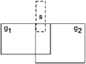
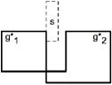
(a)	(b)
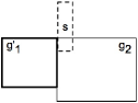
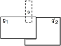
(c)	(d)

Figure 18:  Core vs. consistent answers

5.2 Computing the Core

We now give a characterization of the core of a database instance for a set of SICs of the form (9), which is not explicitly based on the computation of minimal repairs. This equivalent and alternative characterization of the core allows us to compute the core without having to compute all the minimal repairs.

To simplify the notation, we introduce a logical formula that captures a conflict around a tuple of relation $R\in{\it D}$ and a SIC of the form (9) with topological predicate $T$:

$$\forall\bar{x}_{1}\bar{x}_{2}s_{1}s_{2}({\it Confl}_{{\it D},R,T}(\bar{x}_{1},s_{1},\bar{x}_{2},s_{2}) \equiv (R(\bar{x}_{1};s_{1})~{}\wedge~{}R(\bar{x}_{2};s_{2})~{}\wedge\bar{x}_{1}\neq\bar{x}_{2}~{}\wedge~{}{\it T}(s_{1},s_{2}))).$$ (12)

Definition 12

Let ${\it D}$ be a database instance and $\Psi$ a set of SICs of the form (9). For the core ${\it D}^{\star}$ of ${\it D}$ with respect to $\Psi$, it holds ${\it D}^{\star}={\it D}^{\star}_{{\it IIntersects}}\cap{\it D}^{\star}_{{\it Intersects}}\cap{\it D}^{\star}_{{\it Equal}}$, where:

• ${\it D}^{\star}_{{\it IIntersects}}=\{R(\bar{a};{\it Difference}(g,t))~{}|~{}R(\bar{a};g)\in{\it D},t=\bigcup\{g^{\prime}~{}|~{}\textrm{for every}R(\bar{b},g^{\prime})\in{\it D}\textrm{ such that }{\it D}\models{{\it C}onfl}_{{\it D},R,{\it IIntersects}}(\bar{a},g,\bar{b},g^{\prime})\}\}$, where $\bigcup$ is the geomUnion operator that calculates the geometric union (spatial aggregation) of geometries.

• ${\it D}^{\star}_{{\it Intersects}}=\{R(\bar{a};{\it Difference}(g,t))~{}|~{}R(\bar{a};g)\in{\it D},t=\bigcup\{{\it Buffer}(g^{\prime},d)$ $~{}|~{}\textrm{for every }$ $R(\bar{b},g^{\prime})\in{\it D}\textrm{ such that }{\it D}\models{{\it C}onfl}_{{\it D},R,{\it Intersects}}(\bar{a},g,\bar{b},g^{\prime})\}\}$.

• ${\it D}^{\star}_{{\it Equal}}=\{R(\bar{a};g)~{}|~{}R(\bar{a},g)\in{\it D},\textrm{it does not exists }(R(\bar{b},g)\in{\it D},{\it D}\models{{\it C}onfl}_{{\it D},R,{\it Equal}}(\bar{a},g,\bar{b},g))\}$. $\Box$

Notice that $t$ is the union of all the geometries that are in conflict with a given geometry $g$. It is obtained by using the spatial aggregation operator geomUnion.

Now, we give the specification of the cores: ${\it D}^{\star}_{{\it Intersects}}$, ${\it D}^{\star}_{{\it IIntersects}}$, and ${\it D}^{\star}_{{\it Equal}}$ as views in a spatial SQL language. In the following specification, we assume a database instance ${\it D}$ with a relational predicate $R({\it id;geometry})$ and primary key $id$. The following specification shows that our methodologies could be implemented on top of current spatial database management systems. In particular, the definition of ${\it D}^{\star}_{{\it Intersects}}$ uses a fixed value $d$ that represents the minimum distance between geometries in the cartographic scale of the database instance. The intersection of these views makes ${\it D}^{\star}$.

Table 4 shows three views that enables to compute the core of the database with a database predicate $R({\it idl;geometry})$.

${\it D}^{\star}_{{\it Intersects}}$	CREATE VIEW ${\it Core\_Intersects}$ AS $($SELECT ${\it r_{1}.id}$ AS ${\it id}$, difference(${\it r_{1}.geometry}$, Buffer(geomunion(${\it r_{2}.geometry}),d$)) AS ${\it geometry}$ FROM $R$ AS $r_{1}$, $R$ AS $r_{2}$ WHERE ${\it r_{1}.id<>r_{2}.id}$ AND Intersects(${\it r_{1}.geometry,r_{2}.geometry}$) GROUP BY ${\it r_{1}.id}$, ${\it r_{1}.geometry}$ UNION SELECT ${\it r_{1}.id}$ AS ${\it id}$, ${\it r_{1}.geometry}$ AS ${\it geometry}$ FROM $R$ AS $r_{1}$ WHERE NOT EXISTS (SELECT ${\it r_{2}.id,r_{2}.geometry}$ FROM $R$ AS $r_{2}$ WHERE ${\it r_{1}.id<>r_{2}.id}$ AND Intersects$({r_{1}.geometry,r_{2}.geometry})))$
${\it D}^{\star}_{{\it IIntersects}}$	CREATE VIEW ${\it Core\_IIntersects}$ AS $($SELECT ${\it r_{1}.id}$ AS ${\it id}$, difference(${\it r_{1}.geometry}$, geomunion(${\it r_{2}.geometry}))$ AS ${\it geometry}$ FROM $R$ AS $r_{1}$, $R$ AS $r_{2}$ WHERE ${\it r_{1}.id<>r_{2}.id}$ AND Intersects(${\it r_{1}.geometry,r_{2}.geometry}$) AND NOT Touches(${\it r_{1}.geometry,r_{2}.geometry}$) GROUP BY ${\it r_{1}.id}$, ${\it r_{1}.geometry}$ UNION SELECT ${\it r_{1}.id}$ AS ${\it id}$, ${\it r_{1}.geometry}$ AS ${\it geometry}$ FROM $R$ AS $r_{1}$ WHERE NOT EXISTS (SELECT ${\it r_{2}.id,r_{2}.geometry}$ FROM $R$ AS $r_{2}$ WHERE ${\it r_{1}.id<>r_{2}.id}$ AND Intersects(${\it r_{1}.geometry,r_{2}.geometry}$) AND NOT Touches(${\it r_{1}.geometry,r_{2}.geometry})))$
${\it D}^{\star}_{{\it Equal}}$	CREATE VIEW ${\it Core\_Equal}$ AS $($SELECT ${\it r_{1}.id}$ AS ${\it id}$, ${\it r_{1}.geometry}$ AS ${\it geometry}$ FROM $R$ AS $r_{1}$ WHERE NOT EXISTS (SELECT ${\it r_{2}.id,r_{2}.geometry}$ FROM $R$ AS $r_{2}$ WHERE ${\it r_{1}.id<>r_{2}.id}$ AND Equals$({\it r_{1}.geometry,r_{2}.geometry})))$

Table 4: SQL statements to compute views for ${\it D}^{\star}_{{\it Intersects}}$, ${\it D}^{\star}_{{\it IIntersects}}$, and ${\it D}^{\star}_{{\it Equal}}$

Example 16

(example 10 cont.) The example considers only the relation LandP with primary key $idl$ and the SIC (3) of Example 2. We want to consistently answer the query of Example 11, i.e., $\exists{\it name~{}owner}({\it LandP}$ ${{\it(}idl,name,owner;geometry)}~{}$ $\wedge$ ${{\it I}Intersects(geometry},([x_{1},y_{1}],[x_{2},y_{1}],[x_{2},y_{2}],[x_{1},y_{2}],[x_{1},y_{1}])).$

To answer this query, we generate a view of the ${\it core}$ applying the definition in Table 4. That is, we eliminate from each geometry the union of conflicting regions with respect to each land parcel. In this case, the conflicting geometries for $g_{2}$ are $g_{3}$ and $g_{4}$; for geometry $g_{3}$ is $g_{2}$; and for geometry $g_{4}$ is $g_{2}$. This is the definition of the core in SQL:

CREATE VIEW $$Core$$

AS (SELECT $$l_{1}.idl\textrm{ AS }idl,l1.name\textrm{ AS }name,l_{1}.owner\textrm{ AS }owner,$$

$${\it difference}(l_{1}.geometry,{\it geomunion}(l_{2}.geometry))\textrm{ AS }geometry$$

FROM $$LandP\textrm{ AS }l_{1},LandP\textrm{ AS }l_{2}$$

WHERE $$l_{1}.idl<>l_{2}.idl\textrm{ AND }{\it Intersects}(l_{1}.geometry,l_{2}.geometry)\textrm{ AND}$$

$$\textrm{NOT}{\it Touches}(l_{1}.geometry,l_{2}.geometry)$$

GROUP BY $$l_{1}.idl,l_{1}.name,l_{1}.owner,l1.geometry$$

UNION

SELECT $$l_{1}.idl\textrm{ AS }idl,l_{1}.name\textrm{ AS }name,l_{1}.owner\textrm{ AS }owner,l_{1}.geometry\textrm{ AS }geometry$$

FROM $$LandP\textrm{ AS }l_{1}$$

WHERE $$\textrm{NOT EXISTS}\textrm{(SELECT }l_{2}.idl,l_{2}.geometry$$

$$\textrm{FROM }LandP\textrm{ AS }l_{2}$$

$$\textrm{WHERE }l_{1}.idl<>l_{2}.idl\textrm{ AND }{\it Intersects}(l_{1}.geometry,l_{2}.geometry)\textrm{ AND}$$

$$\textrm{NOT}{\it Touches}(l_{1}.geometry,l_{2}.geometry)))$$

We now can pose the query to the core to compute the consistent answer to the original query:

SELECT $${\it idl,name,owner,geometry}$$

FROM $${\it Core}$$

WHERE $${\it Intersects}({\it geometry},([x_{1},y_{1}],[x_{2},y_{1}],[x_{2},y_{2}],[x_{1},y_{2}],[x_{1},y_{1}]))\vspace{-8mm}$$

The answer is shown in Figure 12. This query is a classic selection from the ${\it Core}$ view. $\Box$

This core-based method allows us to compute consistent answers in polynomial (quadratic) time (in data complexity) in cases where there can be exponentially many repairs. In Example 8, where we have $2^{n-1}$ minimal repairs, we can apply the query ${\cal Q}$ over the core, and we only have to compute the difference of a geometry with respect to the union of all other geometries in conflict. This corresponds to a polynomial time algorithm of order polynomial with respect to the size of the database instance.

6 Experimental Evaluation

In this section we analyze the results of the experimental evaluation we have done of the core-based CQA using synthetic and real data sets. The experiment includes a scalability analysis that compares the cost of CQA with increasing numbers of conflicting tuples and increasing sizes of database instances. We compare these results with respect to the direct evaluation of basic conjunctive queries over the inconsistent database (i.e., ignoring inconsistencies). The latter reflects the additional cost of computing consistent answers against computing queries that ignore inconsistencies.

6.1 Experimental Setup

We create synthetic databases to control the size of the database instance and the number of conflicting tuples. We use a database schema consisting of a single predicate $R({{\it i}d};{{\it g}eometry})$, where ${\it id}$ is the numeric key and ${\it geometry}$ is a spatial attribute of type polygon. We create three sets of synthetic database instances by considering SICs of the form (9) with different topological predicates:

Set	SIC
Equals	$\overline{\forall}~{}\neg(R(\bar{x_{1}};s_{1})~{}\wedge~{}R(\bar{x_{2}};s_{2})~{}\wedge~{}\bar{x_{1}}\neq\bar{x_{2}}~{}\wedge~{}\it{Equals}(s_{1},s_{2}))$
Intersects	$\overline{\forall}~{}\neg(R(\bar{x_{1}};s_{1})~{}\wedge~{}R(\bar{x_{2}};s_{2})~{}\wedge~{}\bar{x_{1}}\neq\bar{x_{2}}~{}\wedge~{}\it{Intersects}(s_{1},s_{2}))$
IIntersects	$\overline{\forall}~{}\neg(R(\bar{x_{1}};s_{1})~{}\wedge~{}R(\bar{x_{2}};s_{2})~{}\wedge~{}\bar{x_{1}}\neq\bar{x_{2}}~{}\wedge~{}\it{IIntersects}(s_{1},s_{2}))$

For each set we create five consistent instances including 5,000, 10,000, 20,000, 30,000, and 40,000 tuples of homogeneously distributed spatial objects whose geometries are rectangles (i.e., 5 points per geometric representation of rectangles). Then, we create inconsistent instances with respect to the corresponding SICs in each set with 5%, 10%, 20%, 30%, and 40% of tuples in conflict. For database instances with a SIC and topological ${\it Equals}$, we create inconsistencies by duplicating geometries in a percentage of geometries. For database instances with a SIC and topological ${\it IIntersects}$, we create inconsistencies by making geometries overlap. Finally, for database instances with a SIC and topological ${\it Intersects}$, we create inconsistencies by making a percentage of geometries to touch.

Due to the spatial distribution of rectangles in the sets, the cores for database instances with SICs using topological predicates in $\{{\it Intersects,IIntersects}\}$ have the same numbers of points in their geometric representations than their original instances. For the set of database instances with SICs using topological predicate Equals, the numbers of points in the geometric representations of their cores are less than in the original databases, because we eliminate geometries as we restore consistency. Thus, we are not introducing additional storage costs in our experiments.

To have a better understanding of the computational cost of CQA, we also evaluate the cost of CQA over real and free available data of administrative boundaries of Chile [1]. Chilean administrative boundaries have complex shapes with many islands, specially, in the South of Chile (e.g., a region can have 891 islands). For the real database, we have two predicates ${\it Counties}$ and ${\it Provinces}$. Notice that, at the conceptual label, ${\it Provinces}$ are aggregations of ${\it Counties}$. In this experiment, however, we have used the source data as it is, creating separated tables for ${\it Counties}$ and ${\it Provinces}$ with independent spatial attributes. For this real database, we consider SIC of the form: $\overline{\forall}~{}\neg({\it R}(\bar{x_{1}};s_{1})~{}\wedge~{}{\it R}(\bar{x_{2}};s_{2})~{}\wedge~{}\bar{x_{1}}\neq\bar{x_{2}}~{}\wedge~{}\it{IIntersects}(s_{1},s_{2}))$, with $R$ being ${\it Counties}$ or ${\it Provinces}$.

Table 5 summaries the data sets for the experimental evaluation. The percentage of inconsistency is calculated as the number of tuple in any conflict over the total number of tuples. The geometric representation size is calculated as the number of points in the boundaries of a region.

Source	Name	Tuples	Inconsistency (%)	Geometric representation size
Synthetic	Equals	5,000-40,000	5-40	25,000-200,000
	IIntersects	5,000-40,000	5-40	25,000-200,000
	Intersects	5,000-40,000	5-40	25,000-200,000
Real	Provinces	52	59	35,436
	Counties	307	12.7	72,009

Table 5: Data sets of the experimental evaluation

We measure the computational cost in terms of seconds needed to compute the SQL statement on a Quad Core Xeon X3220 of 2.4 GHz, 1066 MHz, and 4 GB in RAM. We use as spatial DBMS PostgreSQL 8.3.5 with PostGIS 1.3.5.

6.2 Experimental Results

Figure 19 shows the cost of the core computation for the different synthetic database instances. To make this experimental evaluation easier and faster, we used materialized views so that we computed only once the core and applied queries on this core’s view. However, we added the computational cost of the core to each individual query result to have a better understanding of the cost of applying CQA.

The time cost of computing the core for inconsistent databases with respect to a SIC with a topological predicate ${\it Equals}$ decreases as the number of tuples in conflicts increases, since the core eliminates geometries in conflict and, therefore, these empty geometries are then ignored in geometric computations. The cost of computing the core is largely due to the spatial join given by the topological predicate of a SIC, which could decrease using more efficient algorithms and spatial indexing structures.

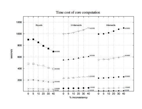
Figure 19: Time cost of the core computation for different SICs, different levels of inconsistency, and different sizes of databases instances

For the synthetic database instance, Figures 20 and 21 show the cost rate between computing a CQA with respect to simple range or join queries (with the spatial predicate Intersects) that ignore inconsistencies. Range queries use a random query window created by a rectangle whose side is equivalent to 1% of the total length in each dimension. Notice that the time cost of computing a range query for a database instance with 10,000 was approximately 15 ms, which, in average, was 900 times less than computing a join query. These reference values exhibit linear and quadratic growth for range and join queries, respectively, as we consider increasing sizes of database instances. The computational cost of CQA to join queries include the computation of the core; however, this cost could be amortized if we use a materialized view of the core for computing more than one join query. In the time cost of CQA for range queries, we have optimized the computation by applying the core-computation over a subset of tuples previously selected by the query range. This optimization is not possible for join queries, since no spatial window can constrain the possible geometries in the answer.

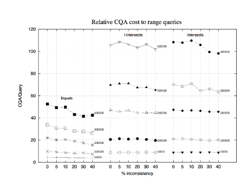
Figure 20: Relative cost of CQA to range queries

Figure 21: Relative cost of CQA to join queries

The results indicate that CQA to a range query can cost 100 times the cost of a simple query. This is primarily due to the join computation of the core. Indeed, when comparing the CQA to a join query, we only duplicate the relative cost, and in the best case, keep the same cost. However, join queries have a significant larger computational cost. Notice that the computation cost for a CQA to range query is around 60s in the worst case (40,000 tuples). With exception of cases when the core contains empty geometries, the percentage of inconsistencies does not affect drastically the results.

We also evaluate the scalability of the CQA cost to range queries in function of the size of the query window (i.e., spatial window). In Figure  22 we show the relative CQA cost to range queries on a synthetic database instance with 10,000 tuples and range queries whose random spatial windows varied from 1% to 5% of the size in each dimension. The results indicate that the relative cost increases logarithmical as we increase the size of the query window. Also, only for database instances with a SIC and topological predicate ${\it Equals}$, the relative cost suffers some variation across different percentages of inconsistencies, primarily, due to the elimination of geometries in the database.

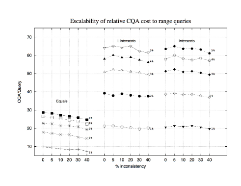
Figure 22: Relative cost of CQA to range queries and different sizes of the query window (using a database instance with 10,000 tuples )

Finally, we applied the core-based computation of CQA to the real database instances in Table 5. Table 6 summaries the results obtained with these data, which were in agreement with the results obtained with the synthetic database instances. In this table, $\Delta{\it Points}$ represents the relative difference in the size of the geometric representation between the core and the original database. Notice that computing the core increased the geometric representation of ${\it Provinces}$ up to 5.0%, which is bounded by the shape of geometries in conflict (i.e., the size of the original geometric representation). In the case of ${\it Counties}$, however, the size of the geometric representation of the core decreases down to $-0.03\%$. Since the geometry of provinces should be the geometric aggregation of counties, we could expect to have a relationship between $\Delta{\it Points}$ for ${\it Provinces}$ and ${\it Counties}$. However, the source data set uses independent geometries for ${\it Provinces}$ and ${\it Counties}$ and no comparison can be made.

			Range		Join
Data	$\Delta$ Points	Core	Simple	CQA	Simple	CQA
Provinces	+5.0%	17.7	0.04	0.25	29.8	63.4
Counties	-0.03%0	18.1	0.1	2.1	40.6	55.7

Table 6: CQA cost with real data (costs of core and queries in seconds)

7 Conclusions

We have formalized a repair semantics and consistency query answers for spatial databases with respect to SICs. The repair semantics is used as an auxiliary concept for handling inconsistency tolerance and computing consistent answers to spatial queries. It is based on updates that shrink geometries of objects, even at the point of deleting geometries for some exceptional cases, as for predicate Disjoint. Geometries are virtually updated applying admissible geometric operators, which are available in most spatial DBMSs.

By restricting ourselves to the application of the admissible transformations, we have a finite number of possibilities for making a pair of geometries consistent with respect to a SIC. However, there may still be exponentially many repairs for a given instance and set of SICs. With the purpose of avoiding to compute and query all repairs, we have identified cases of SICs and conjunctive (range and join) queries where the consistent answers can be obtained by posing a standard query to a single view of the original instance. This view is equivalent to the intersection of all possible minimal repairs, what we called the ${\it core}$ of a database instance, which for a subset of SICs can be computed in polynomial time without determining each repair.

An experimental evaluation of the core-based computation of CQA reveals that answering range queries has a cost that varies drastically in function of the topological predicates in SICs and the number of tuples in the database instance, reaching up to 100 times the cost of a simple range query. This is mainly due to the spatial join involved in computing the core. For join queries, instead, the cost of CQA is the double of a simple join query. These results do not use optimizations with spatial indexing, which has been left for future work. Even more, they assume that we have to compute the core for each query, which could be optimized by using materialized views.

This work leaves many problems open. Most prominently, computability and complexity issues have to be explored. For example, some interesting decision problems are deciding if non trivial repairs (i.e., not obtained by cancellation of geometries) exist for an instance and a set of SICs, or deciding whether or not a particular instance is a repair of an inconsistent database instance. The complexity of deciding if a spatio-relational tuple is a consistent answer is also open. As in the relational case, we expect to find hard cases for all these problems. For them, it would be interesting to obtain lower complexity approximation algorithms.

We have considered only regions to represent spatial objects. A natural extension of this work would be to define a repair semantics for other spatial abstractions, such as polylines, points, networks, and so on. We would also like to explore not only denial SICs, but also other classes of semantic ICs, and other types of repair semantics that include solving conflicts with respect to a topological predicate ${{\it D}isjoint}$. This includes also the possibility of considering combinations of spatial with relational constraints, e.g. functional dependencies and referential ICs.

Acknowledgments

This project is partially funded by FONDECYT, Chile, grant number 1080138. Part of this research was done when L. Bertossi was invited to the Universidad de Concepcion and Universidad del Bío-Bío. Mónica Caniupán received funding from FONDECYT, Chile, grant number 11070186. Leopoldo Bertossi has also been partially funded by an NSERC Discovery Grant (#315682).

References

- [1] Albers, C. Gisdata chile, administrative boundaries since 2007. http://www.rulamahue.cl/mapoteca/catalogos/chile.html, 2009.
- [2] Arenas, M., Bertossi, L., and Chomicki, J. Consistent query answers in inconsistent databases. In 18th ACM Symposium on Principles of Database Systems PODS’99 (1999), ACM Press, pp. 68–79.
- [3] Arenas, M., Bertossi, L., and Chomicki, J. Scalar aggregation in fd-inconsistent databases. In Proc. International Conference on Database Theory (2001), Springer LNCS 1973, pp. 39–53.
- [4] Bertossi, L. Consistent query answering in databases. ACM Sigmod Record 35, 2 (2006), 68–76.
- [5] Bertossi, L., and Bravo, L. Consistent query answers in virtual data integration systems. In Inconsistency Tolerance (2005), vol. 3300 of Lecture Notes in Computer Science, Springer, pp. 42–83.
- [6] Bertossi, L., and Chomicki, J. Logics for Emerging Applications of Databases. Springer, 2003, ch. Query Answering in Inconsistent Databases, pp. 43–83.
- [7] Bertossi, L., Hunter, A., and Schaub, T., Eds. Inconsistency Tolerance (2005), vol. 3300 of Lecture Notes in Computer Science, Springer.
- [8] Borges, K., Laender, A., and Davis, C. Spatial integrity constraints in object oriented geographic data modeling. In ACM International Symposium on Advances in GIS (1999), ACM Press, pp. 1–6.
- [9] Caniupan, M. Optimizing and Implementing Repair Programs for Consistent Query Answering in Databases. PhD thesis, Carleton University, Department of Computer Science, 2007.
- [10] Chomicki, J. Consistent query answering: Five easy pieces. In International Conference on Database Theory ICDT’07 (2007), vol. LNCS 4353, Springer-Verlag, pp. 1–17.
- [11] Cockcroft, S. A taxonomy of spatial integrity constraints. GeoInfomatica 1, 4 (1997), 327–343.
- [12] Duckham, M., Lingham, J., Mason, K. T., and Worboys, M. F. Qualitative reasoning about consistency in geographic information. Inf. Sci. 176, 6 (2006), 601–627.
- [13] Egenhofer, M., Clementine, E., and Felice, P. D. Evaluating inconsistency among multiple representations. In Spatial Data Handling (1995), pp. 901–920.
- [14] Egenhofer, M., and Sharma, J. Assessing the consistency of complete and incomplete topological information. Geographical Systems 1 (1993), 47–68.
- [15] Egenhofer, M. J., and Franzosa, R. D. Point set topological relations. International Journal of Geographical Information Systems 5 (1991), 161–174.
- [16] Franconi, E., Palma, A. L., Leone, N., Perri, S., and Scarcello, F. Census data repair: a challenging application of disjunctive logic programming. In LPAR (2001), R. Nieuwenhuis and A. Voronkov, Eds., vol. 2250 of Lecture Notes in Computer Science, Springer, pp. 561–578.
- [17] Fuxman, A., Fazli, E., and Miller, R. J. Conquer: Efficient management of inconsistent databases. In SIGMOD Conference (2005), F. Özcan, Ed., ACM, pp. 155–166.
- [18] Güting, R. H. Graphdb: Modeling and querying graphs in databases. In VLDB (1994), J. B. Bocca, M. Jarke, and C. Zaniolo, Eds., Morgan Kaufmann, pp. 297–308.
- [19] Güting, R. H., and Schneider, M. Realm-based spatial data types: The rose algebra. VLDB J. 4, 2 (1995), 243–286.
- [20] Hadzilacos, T., and Tryfona, N. A model for expressing topological integrity constraints in geographic databases. In Spatio-Temporal Reasoning (1992), A. U. Frank, I. Campari, and U. Formentini, Eds., vol. 639 of Lecture Notes in Computer Science, Springer, pp. 252–268.
- [21] Kuijpers, B., Paredaens, J., and den Bussche, J. V. On topological elementary equivalence of spatial databases. In ICDT (1997), F. N. Afrati and P. G. Kolaitis, Eds., vol. 1186 of Lecture Notes in Computer Science, Springer, pp. 432–446.
- [22] Mäs, S. Reasoning on spatial semantic integrity constraints. In COSIT (2007), S. Winter, M. Duckham, L. Kulik, and B. Kuipers, Eds., vol. 4736 of Lecture Notes in Computer Science, Springer, pp. 285–302.
- [23] OpenGis. Opengis simple features specification for sql. Tech. rep., Open GIS Consortium, 1999.
- [24] Paredaens, J., den Bussche, J. V., and Gucht, D. V. Towards a theory of spatial database queries. In PODS (1994), ACM Press, pp. 279–288.
- [25] Paredaens, J., and Kuijpers, B. Data models and query languages for spatial databases. Data Knowl. Eng. 25, 1-2 (1998), 29–53.
- [26] Randell, D. A., Cui, Z., and Cohn, A. G. A spatial logic based on regions and connection. In KR (1992), pp. 165–176.
- [27] Rodríguez, M. A. Inconsistency issues in spatial databases. In Inconsistency Tolerance (2005), vol. 3300 of Lecture Notes in Computer Science, Springer, pp. 237–269.
- [28] Rodríguez, M. A., Bertossi, L., and Caniupan, M. An inconsistency tolerant approach to querying spatial databases. In ACM-GIS (2008), W. G. Aref, M. Mokbel, and M. Schneider, Eds., ACM.
- [29] Servige, S., Puricelli, T., and Laurini, R. A methodology for spatial consistency improvement of geographic databases. GeoInformatica 4 (2000), 7–24.
- [30] Thompson, D., and Laurini, R. Fundamentals of Spatial Information Systems. No. 37 in APIC. Academic Press, 1992.
- [31] Tryfona, N., and Egenhofer, M. Consistency among parts and aggregates: A computational model. Transactions on GIS 1, 1 (1997), 189–206.
- [32] Wijsen, J. Database repairing using updates. ACM Trans. Database Syst. 30, 3 (2005), 722–768.