Charged Particle Motion in a Plasma:
Electron-Ion Energy Partition

Abstract

This paper considers plasmas in which the electrons and ions may have different temperatures. This is a case that must be examined because nuclear fusion processes, such as those that appear in ICF capsules, have ions whose temperature runs away from the electron temperature. A fast charged particle traversing a plasma loses its energy to both the electrons and the ions in the plasma. We compute the energy partition, the fractions $E_{e}/E_{0}$ and $E_{\rm\scriptscriptstyle I}/E_{0}$ of the initial energy $E_{0}$ of this ‘impurity particle’ that are deposited into the electrons and ions when it has slowed down into a “schizophrenic” final ensemble of slowed particles that has neither the electron nor the ion temperature. This is not a simple Maxwell-Boltzmann distribution since the background particles are not in thermal equilibrium. We perform our calculations using a well-defined Fokker-Planck equation for the phase space distribution of the charged impurity particles in a weakly to moderately coupled plasma. The Fokker-Planck equation holds to first sub-leading order in the dimensionless plasma coupling constant, which translates to computing to order $n\ln n$ (leading) and $n$ (sub-leading) in the plasma density $n$. An examination of the energy partition for the general case, in which the background plasma contains two different species of particles that are not in thermal equilibrium, has not been previously presented in the literature. We have new results for this case. The energy partitions for a background plasma in thermal equilibrium have been previously computed, but the order $n$ terms have not been calculated, only estimated. Since the charged particle does not come to rest, but rather comes into a statistical distribution, the energy loss obtained by a simple integration of a $dE/dx$ has an ambiguity on the order of the plasma temperature. Our Fokker-Planck formulation provides an unambiguous, precise definition of the energy fractions. For equal electron and ion temperatures, we find that our precise results agree well with a fit obtained by Fraley, Linnebur, Mason, and Morse. The “schizophrenic” final ensemble of slowed particles gives a new mechanism to bring the electron and ion temperatures together. The rate at which this new mechanism brings the electrons and ions in the plasma into thermal equilibrium will be computed.

I Introduction

The underlying theme of this paper is the thermonuclear burn of deuterium-tritium plasmas. We do not consider the initiation of the burn process, which is system specific, nor are we interested in the late stages of the process when most of the DT fuel has been burned into alpha particles and neutrons, and the electrons and ions are nearly in thermal equilibrium. We instead focus on intermediate times when, in general, there is a significant difference between the electron and ion temperatures, but the alpha particle density has not yet become a significant fraction of the D and T ion densities. The fusion rate is very sensitive to the ion temperature $T_{\rm\scriptscriptstyle I}$. The ion temperature is determined by competition between deposition of the alpha particle energy into the ions, which of course increases $T_{\rm\scriptscriptstyle I}$, and thermal equilibration with the electron distribution, which drives $T_{\rm\scriptscriptstyle I}$ down. Our main concern in this paper is the partition of the total alpha energy between the ions and electrons in a two-temperature plasma in the circumstances that we have outlined. This is important in the understanding of the time scale and the robustness of the fusion process. Our evaluations of the functions which determine the energy partition do not include a contribution from the alpha particles; hence our results are valid only if the ensemble of alphas is sufficiently dilute. We find that the alpha particles slow down into a non-Maxwellian distribution in which the mean alpha energy $\bar{E}$ lies between the thermal energies of the ions and electrons. Our work shows that these non-thermal alpha particles increase the rate of energy transfer between the electrons and ions but, since we do not examine late times where the population of alpha particles is large, this new mechanism does not significantly enhance the energy transfer rate. In general, as in other work on stopping power and the partition of a fast impurity particle’s energy to the electrons and ions in the plasma, we assume (as is most often the case) that the stopping times are much shorter than the time scale of the fusion so that we can work in the adiabatic approximation in which the time dependences of our results are only those brought about by the changes in the plasma parameters on which they depend. We also require, as is also generally assumed, that the charged particle range is short in comparison with the distances over which the plasma conditions vary so that the plasma may be treated as being uniform.

The major results of this paper are as follows. First, as we have mentioned in the previous paragraph, we have worked out the energy partition for differing electron and ion temperatures; this has not been previously considered in the literature. Second, even for the case of equal ion and electron temperatures, where the alphas relax into a Maxwellian distribution, we have made two improvements. We have developed a formulation that precisely defines the energy partition so that a correction of order $T/E_{0}$ is now included, a correction that is missing in the literature. In addition to the well-known $n\,\ln\,n$ ($n$ is the number density) terms in the energy partition, we have computed exactly the coefficient of the order $n$ term, which has previously been only estimated. We turn now to describe our work in some detail.

When a fast charged particle with initial energy $E_{0}$ traverses a plasma, it loses its energy at a rate $dE/dx$ per unit of distance, and it comes into a quasi-static equilibrium state after depositing its initial energy into the electrons and ions that make up the plasma. In the thermonuclear fusion process of deuterium and tritium, $D+T\to n+\alpha$, which occurs in inertial confinement fusion experiments, the amount of the initial alpha-particle energy $E_{0}=3.54$ MeV that is transferred to the $D,T$ ions is crucial because a high ion temperature is necessary for the fusion reaction parameter $\langle\sigma\,v\rangle_{\rm\scriptscriptstyle T}$ to become sufficiently large so as to have a robust and stable fusion burn.

In the picture in which the projectile traverses linearly through the plasma until coming to a complete stop, the energy partition into ions and electrons is given by

$$E_{\rm\scriptscriptstyle I}=\int_{0}^{E_{\rm\scriptscriptstyle I}}\!dE_{\rm\scriptscriptstyle I}=\int_{0}^{E_{0}}\!dE~{}\frac{dE_{\rm\scriptscriptstyle I}/dx}{dE/dx}\,,$$ (1)

and

$$E_{e}=\int_{0}^{E_{e}}\!dE_{e}=\int_{0}^{E_{0}}\!dE~{}\frac{dE_{e}/dx}{dE/dx}\,.$$ (2)

Here $dE_{\rm\scriptscriptstyle I}/dx$ and $dE_{e}/dx$ are the stopping power contributions from the ions and electrons, and $dE/dx$ is the total stopping power,

$$\frac{dE}{dx}=\frac{dE_{\rm\scriptscriptstyle I}}{dx}+\frac{dE_{e}}{dx}\,,$$ (3)

and thus

$$E_{\rm\scriptscriptstyle I}+E_{e}=E_{0}\,.$$ (4)

This simple picture, however, is only an approximation. For a plasma with equal ion and electron temperatures, a fast charged particle does not simply come to rest in the plasma, but rather, it becomes thermalized at the ambient plasma temperature $T=T_{\rm\scriptscriptstyle I}=T_{e}$. Expressing temperature in energy units, as we shall do throughout this paper, the correct electron-ion energy partition relation should read

$$E_{\rm\scriptscriptstyle I}+E_{e}+\frac{3}{2}\,T=E_{0}\,.$$ (5)

Consequently, rather than extending the lower limits of the integrals (1) and (2) down to zero energy, lower limits of order the temperature, $E_{\text{min}}\sim T$, must be chosen. The two integrals (1) and (2) have somewhat different thermal cutoffs, both of order $T$, and this simple picture has a systematic error of relative order $T/E_{0}$. We see that the correction becomes more important as the plasma temperature is elevated. To account for the energy partition in a precise fashion, we shall employ the Fokker-Planck equation in the version introduced by Brown, Preston, and Singleton (BPS) bps . We shall find that the correct expression for the energy partition does not, in fact, involve the stopping powers $dE_{\rm\scriptscriptstyle I}/dx$ and $dE_{e}/dx$, but rather certain ion and electron functions ${\cal A}_{\rm\scriptscriptstyle I}$ and ${\cal A}_{e}$ that enter into this Fokker-Planck equation. In the notation of BPS, the stopping power of a particle of energy $E=\frac{1}{2}\,m\,v^{2}$ is of the generic form

$$\frac{dE_{a}}{dx}=\left[1-\frac{T}{mv}\,\frac{\partial}{\partial{\bf v}}\,\cdot\hat{\bf v}\right]\,{\cal A}_{a}\,.$$ (6)

The functions ${\cal A}_{\rm\scriptscriptstyle I}$ and ${\cal A}_{e}$ thus approach $dE_{\rm\scriptscriptstyle I}/dx$ and $dE_{e}/dx$ at high energies, but differ from these stopping powers at low energies on the order of the thermal background temperature.

For the case of equal electron and ion temperatures, the explicit evaluations for $E_{\rm\scriptscriptstyle I}$ and $E_{e}$ derived in Eqs. (121) and (122), which omit of negligibly small exponential terms involving $\exp\{-\beta E_{0}\}$, read:

$$E_{\rm\scriptscriptstyle I} = \int_{0}^{E_{0}}dE\,\,\frac{{\cal A}_{\rm\scriptscriptstyle I}(E)}{{\cal A}(E)}\left[{\rm erf}(\sqrt{\beta E})-\sqrt{\frac{4\beta E}{\pi}}\,e^{-\beta E}\right]\,,$$ (7)

and

$$E_{e} = \int_{0}^{E_{0}}dE\,\,\frac{{\cal A}_{e}(E)}{{\cal A}(E)}\left[{\rm erf}(\sqrt{\beta E})-\sqrt{\frac{4\beta E}{\pi}}\,e^{-\beta E}\right]\,,$$ (8)

where

$${\cal A}(E)={\cal A}_{\rm\scriptscriptstyle I}(E)+{\cal A}_{e}(E)\,,$$ (9)

and $\beta=1/T$. Here ${\rm erf}(x)$ is the error function defined in Eq. (120). Using the definition (120), partial integration can then be used to show that the sum rule (5) follows from Eqs. (7) and (8). Since $dE_{b}/dx\to{\cal A}_{b}$ for large energies, and since the error function approaches unity at large $\beta E$, the precise results (7) and (8) approach the more intuitive but less accurate forms (1) and (2). Significant differences occur only for $E\sim T$.

We have numerically evaluated these integrals using the expressions for the ${\cal A}$ functions derived in BPS that are reproduced in Appendix A. We shall compare our results with the less precise but well known results of Fraley, Linnebur, Mason, and Morse  (FLMM) fraley . Starting with a model of the stopping power in an equimolar DT plasma, these authors show that the simple rule

$$\frac{E_{\rm\scriptscriptstyle I}}{E_{0}}=\frac{1}{1+T_{\rm\scriptscriptstyle C}/T_{e}}$$ (10)

provides a good fit to their calculations. The crossover temperature $T_{\rm\scriptscriptstyle C}$, where the electron and ion fractions are equal, can be determined from their Fig. 1b. Fraley et al. find $T_{\rm\scriptscriptstyle C}=32\,{\rm keV}$ at the density $\rho=0.213\,{\rm g/cm^{3}}$, or a corresponding electron number density $n_{e}=5.0\times 10^{22}\,{\rm cm}^{-3}$. At the number densities $n_{e}=1.0\times 10^{24}\,,\,1.0\times 10^{25}\,,\,1.0\times 10^{26}\,{\rm cm}^{-3}$, we find, by fitting our more precise results, that $T_{\rm\scriptscriptstyle C}=31\,,\,30\,,\,28\,\,{\rm keV}$ respectively. Figure 1 shows our result (7) for the fractional energy loss to ions and the FLMM fit (10) for a DT plasma with electron number density $n_{e}=10^{26}\,{\rm cm}^{-3}$. In this comparison, we use the more accurate value $T_{\rm\scriptscriptstyle C}=28$ keV. In Fig. 2 we compare the differences between our result (7) and the FLMM fit (10) over a wide range of densities. We see that the FLMM fit somewhat overestimates the energy deposited to ions for temperatures above 120 keV over a wide range of densities.

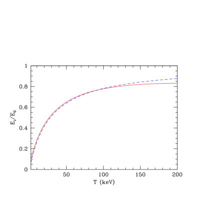
Figure 1: The fractional energy loss into ions as a function of the plasma temperature for an $\alpha$ particle in an equimolar DT plasma with initial energy $E_{0}=3.54\,{\rm MeV}$. The electrons and ions have a common temperature $T$ and the electron number density of the plasma is $n_{e}=1.0\times 10^{26}\,{\rm cm}^{-3}$. The solid red line is the evaluation of Eq. (7) while the dashed blue line is the FLMM fit (10) with $T_{\rm\scriptscriptstyle C}=28\,{\rm keV}$ rather than the $32\,{\rm keV}$ value used by FLMM.

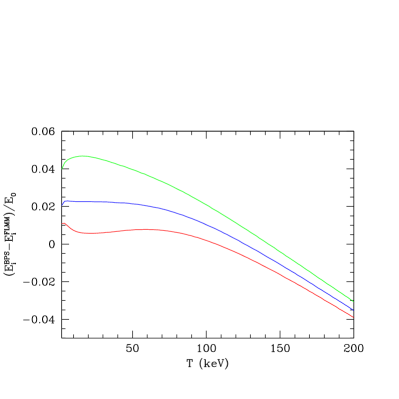
Figure 2: Differences between the fractional energy losses $E_{\rm\scriptscriptstyle I}/E_{0}$ as given by the precise result (7) and the FLMM fit (10) for an alpha particle with initial energy $E_{0}=3.54$ MeV in an equimolar DT plasma. The different curves correspond to the three electron densities $n_{e}$ of $1.0\times 10^{24}\,{\rm cm}^{-3}$ (red), $1.0\times 10^{25}\,{\rm cm}^{-3}$ (blue), and $1.0\times 10^{26}\,{\rm cm}^{-3}$ (green), with the fit (10) evaluated with $T_{\rm\scriptscriptstyle C}=31\,,\,30\,,\,{\rm and}\,\,28\,{\rm keV}$, respectively.

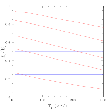
Figure 3: The red curves show the energy fractions deposited to the ions as functions of the ion temperature $T_{\rm\scriptscriptstyle I}$ for various values of the electron temperature $T_{e}$ for an $\alpha$ particle with initial energy $E_{0}=3.54\,{\rm MeV}$ in an equimolar DT plasma with an electron density $n_{e}=1.0\times 10^{25}\,{\rm cm}^{-3}$. The blue horizontal lines are the energy fractions determined by the FLMM fit (10) with our value $T_{\rm\scriptscriptstyle C}=30\,{\rm keV}$. The red curves describing larger values of $E_{\rm\scriptscriptstyle I}/E_{0}$ correspond to increasing electron temperatures of $T_{e}=10\,,\,30\,,\,50\,,\,100\,,\,200\,{\rm keV}$. If the fit (10) were exact, the red curves would cross the blue horizontal lines when $T_{\rm\scriptscriptstyle I}=T_{e}$. This condition is fairly well met except at the highest electron temperature $T_{e}=200$ keV where the value of $E_{\rm\scriptscriptstyle I}/E_{0}$ given by the red curve at $T_{\rm\scriptscriptstyle I}=200$ keV is considerably smaller than the blue horizontal line. This is consistent with the discrepancy at these temperatures shown in Fig. 1.

As Figs. 1 and 2 show, the FLMM fit (10), modified slightly to use better values of the crossover temperature $T_{\rm\scriptscriptstyle C}$, is in good agreement with our precise results in the case of equal temperatures so long as these temperatures are less that about $120$ keV. However, as Fig. 3 demonstrates, this simple form fails to provide an accurate estimate of the energy partition when the ion and electron temperatures are significantly different. These results for differing electron and ion temperatures follow from Eqs. (137) and (139). They are spelled out in more detail in the tables presented in our concluding section V.

Although the work of FLMM continues to be used, a more recent evaluation of the energy partition has been carried out by Li and Petrasso LP . Comparing their Table 1 ($T_{\rm\scriptscriptstyle I}=T_{e}$) with our Fig. 1 shows that their results for $E_{\rm\scriptscriptstyle I}/E_{0}$ are $\sim 10\%$ too high. This discrepancy is of order the sub-leading corrections to the Coulomb logarithm.

The emphasis in this paper is the energy partition for unequal electron and ion temperatures, which is of the utmost importance for DT burn since there the ion temperature generally runs away from the electron temperature once the fusion process begins. To describe this in a simple fashion, we assume that the sources of the charged impurity particles (the $\alpha$ particles in DT fusion) are uniformly distributed throughout the plasma, and that the particles are emitted isotropically; hence, the phase space distribution of the impurity particles is only a function of the energy and time. The evolution of this distribution is governed by a Fokker-Planck equation that involves the coefficient functions ${\cal A}_{\rm\scriptscriptstyle I}(E)$ and ${\cal A}_{e}(E)$ which were computed in BPS to order $n(\ln n+c)$ in the plasma density $n$. Since $n\sim g^{2}$, with $g$ the plasma coupling constant, it is evident that these two terms in the density are the leading and first sub-leading terms in the perturbative expansions in $g$ of the coefficient functions. Higher-order terms in the expansions become significant at high densities, hence our results are not applicable, in particular, to (strongly coupled) warm dense plasmas. Numerical simulations provide the only potentially reliable means of validating our analytic expressions for the energy partition in weakly coupled plasmas and evaluating the partition in moderately to strongly coupled plasmas, though such computations have not been performed. Careful, large statistics, molecular dynamics (MD) simulations have been carried out by Dimonte and Daligault DD to investigate electron-ion temperature relaxation over a wide range of plasma parameters that span weak to strong coupling. Their MD results for the Coulomb logarithm for this process agree with those of BPS bps for $g<0.2$ to within the statistical uncertainty of $\pm 5\%$ in the simulations. This indicates the range of validity of the Fokker-Planck equation that we use to compute a different result, the energy partition.

Following a detailed discussion of the Fokker-Planck equation in Sections II.1 and II.2, the late-time distribution $f_{\infty}(E)$ of a $\delta(t)$ source of impurity particles, which is needed to obtain the electron-ion energy split, is derived in Section II.3. In Section III a source is slowly turned on and eventually emits particles at a constant rate. The solution $f(E,t)$ of the now inhomogeneous Fokker-Planck equation is shown to be the sum of two terms: $f(E,t)=n(t)\,f_{\infty}(E)+\bar{f}(E)$, where $n(t)$ is the number density of impurity particles that have come into the equilibrium state described by $f_{\infty}(E)$, and $\bar{f}(E)$, which describes the transfer of energy to the electrons and ions. The energy losses $E_{e}$ and $E_{\rm\scriptscriptstyle I}$ to the electrons and ions are expressed as single integrals involving the function $\bar{f}(E)$ [which depends upon the ${\cal A}$-coefficients] and the ${\cal A}$-coefficients themselves. The late-time ensemble of impurity particles with energy distribution $f_{\infty}(E)$ is not in thermal equilibrium with the background plasma, i.e. $f_{\infty}(E)$ is not a Maxwell-Boltzmann distribution. This ensemble increases the rate of ion-electron thermal equilibration above that of the impurity-free plasma. In Section IV.1 we carry out the explicit construction of $\bar{f}(E)$. We show how our general results for the deposited energy fractions $E_{\rm\scriptscriptstyle I}$ and $E_{e}$ in the equal temperature case reduce to the usual expressions involving $dE_{\rm\scriptscriptstyle I}/dx$ and $dE_{e}/dx$ in Section IV.2 and then describe how these approximate results are corrected with our precise formulation in Section IV.3. In Section IV.4 we compute $E_{\rm\scriptscriptstyle I}/E_{0}$ and $E_{e}/E_{0}$ for the general case of different plasma electron and ion temperatures in terms of integrals over ${\cal A}_{\rm\scriptscriptstyle I}$ and ${\cal A}_{e}$. The conclusion V provides a summary of our major results including a table of the energy fractions $E_{\rm\scriptscriptstyle I}/E_{0}$ and $E_{e}/E_{0}$ for a wide range of plasma parameters. At this point, we have finished a logically complete exposition of our methodology and results, which is essentially self-contained. However, for those interested in supporting details and who may wish to work out the intermediate steps in our calculations, we include these details in the Appendices. We provide a review of the ${\cal A}$ functions that were computed in BPS bps which are needed for the present work in Appendix A, a host of details on these functions that include their approximate forms in various regions in Appendix B, and an accurate approximation for one of the two multiple integrals appearing in our final expressions for $E_{\rm\scriptscriptstyle I}$ and $E_{e}$ is provided in Appendix C.

II Formulation of the Problem

II.1 The Fokker-Planck Equation to Leading and Next-to-Leading Order

We consider a plasma containing a dilute population of “impurity” particles with a phase space density $f({\bf r},{\bf p},t)$. For example, in a deuterium-tritium (DT) plasma, the impurities could consist of the charged $\alpha$ particles produced from the DT fusion. The problem we shall address is the manner by which such impurities reach a quasi-static equilibrium distribution. During this process, the impurities deposit portions of their energy to plasma electrons and plasma ions, and the formalism we now develop will allow us to compute the electron-ion energy splitting in a systematic and unambiguous fashion. We take the plasma to have an electron temperature $T_{e}=\beta_{e}^{-1}$ and a common temperature $T_{\rm\scriptscriptstyle I}=\beta_{\rm\scriptscriptstyle I}^{-1}$ for all the ions, in which case the Fokker-Planck equation for the distribution $f$ of an impurity species has the form

$$\left[\frac{\partial}{\partial t}+{\bf v}\cdot{\bm{\nabla}}\right]f({\bf r},{\bf p},t)={\sum}_{b}\,\frac{\partial}{\partial p^{k}}\,C_{b}^{k\ell}({\bf p})\left[\beta_{b}v^{\ell}+\frac{\partial}{\partial p^{\ell}}\right]f({\bf r},{\bf p},t)\,,$$ (11)

where ${\bf v}={\bf p}/m$ is the velocity of an impurity particle with momentum ${\bf p}$, the explicit sum runs over all the particle species $b$ in the background plasma, and the summation convention is used for repeated vector indices $k$ and $\ell$. As we shall describe more fully, the diffusion coefficient $C_{b}^{k\ell}$ has been analytically calculated to leading and next-to-leading orders in the plasma density in BPS bps or more precisely, to orders $g^{2}\ln g^{2}$ and $g^{2}$ in the generic dimensionless plasma coupling constant $g=e^{2}\kappa/4\pi T$. We use rationalized electrostatic units, so that this parameter is the Coulomb energy of two particles of charge $e$ a Debye distance $1/\kappa$ apart divided by an average temperature $T$.

With our conventions, the number of impurity particles is given by

$$N(t)=\int d^{3}r\int\frac{d^{3}p}{(2\pi\hbar)^{3}}\,f({\bf r},{\bf p},t)\,,$$ (12)

and their kinetic energy and momentum appear as

$$E(t)=\int d^{3}r\int\frac{d^{3}p}{(2\pi\hbar)^{3}}\,\frac{p^{2}}{2m}\,f({\bf r},{\bf p},t)\,,$$ (13)

and

$${\bf P}(t)=\int d^{3}r\int\frac{d^{3}p}{(2\pi\hbar)^{3}}\,{\bf p}\,f({\bf r},{\bf p},t)\,.$$ (14)

Since the right-hand side of the Fokker-Planck equation (11) contains an overall total momentum derivative, it does not contribute to the time rate of change of the particle number — the Coulomb collisions in the plasma preserve particle number. When the electrons and ions are at common temperature $T=\beta^{-1}$, the terms in the final square brackets in the Fokker-Planck equation (11) annihilate a thermal Maxwell-Boltzmann distribution [$f\propto\exp\{-\beta\,{\bf p}^{2}/2m\}$] of impurity particles — a collection of particles in thermal equilibrium is not altered by their collisions with a background plasma at the same temperature. However, for those cases in which the ions and electrons have different temperatures, the “injected impurity particles” attain a non-thermal quasi-static distribution that will be described shortly. Eventually this quasi-static distribution will relax into a thermal distribution as the electron and ion components themselves thermally relax. As we shall see, however, the impurity distribution has interesting effects on temperature relaxation at intermediate times.

The stopping power can be extracted from the Fokker-Planck equation by considering a single impurity particle at ${\bf r}_{p}$ moving with the velocity ${\bf v}_{p}$. The corresponding distribution function is given by $f_{p}({\bf r},{\bf p},t)=(2\pi\hbar)^{3}\delta({\bf r}-{\bf r}_{p})\delta({\bf p}-{\bf p}_{p}),$ and one can easily check that this distribution indeed gives $N=1$ as it should. Inserting this single particle distribution into Eq. (11) and performing a partial integration, it is easy to see that the rate of energy loss of the particle is given by

$$\frac{dE}{dt}=+{\sum}_{b}\,\left[\beta_{b}v^{\ell}_{p}-\frac{\partial}{\partial p^{\ell}_{p}}\right]\,v^{k}_{p}\,C_{b}^{k\ell}({\bf p}_{p})\,.$$ (15)

To make the sign of this expression clear, we emphasize that it gives the rate at which the particle loses energy to the plasma [it is the negative of the time derivative of Eq. (13)]. Hence the stopping power, which is the energy loss of the particle per unit distance traveled, appears as

$$\frac{dE}{dx}=+\,\frac{1}{v_{p}}\,\frac{dE}{dt}\,.$$ (16)

In a similar manner, we can find the rate of change of the momentum by substituting the single particle distribution into expression (14), thereby giving

$$\frac{dP^{k}}{dt}={\sum}_{b}\,\left[\beta_{b}v^{\ell}_{p}-\frac{\partial}{\partial p^{\ell}_{p}}\right]\,C_{b}^{k\ell}({\bf p}_{p})\,.$$ (17)

As performed in BPS, by calculating $dE/dt$ and $dP^{k}/dt$ to leading and next-to-leading order, we can invert equations (15) and (17) to the same order to obtain the coefficients $C_{b}^{k\ell}$ of the Fokker-Planck equation.

II.2 Longitudinal and Transverse Components of the Diffusion Tensor

As described in detail in BPS, the isotropy of the background thermal plasma allows one to decompose the diffusion tensor as

$$C_{b}^{k\ell}({\bf p})={\cal A}_{b}(v)\,\frac{\hat{v}^{k}\hat{v}^{\ell}}{\beta_{b}v}+{\cal B}_{b}(v)\,\frac{1}{2}\,\left(\delta^{k\ell}-\hat{v}^{k}\hat{v}^{\ell}\right)\,,$$ (18)

where $v$ is the magnitude of the velocity, $v=|{\bf v}|$, with the velocity direction given by $\hat{\bf v}={\bf v}/v$. We often take the independent variable to be the energy $E=\frac{1}{2}\,mv^{2}$ and, with a slight abuse of notation, we shall also write ${\cal A}_{b}={\cal A}_{b}(E)$ and ${\cal B}_{b}={\cal B}_{b}(E)$. As a matter of completeness, the ${\cal A}$-coefficients are provided in Appendix A, and their various limits can be found in Appendix B. For a homogeneous and isotropic source of impurity particles, the case we shall consider, the ${\cal B}$-coefficients do not enter, although their analytic forms can be found in BPS bps if desired.

Let us return to the stopping power (15) of a charged particle. Since the velocity tensor multiplying the ${\cal B}$-contribution is transverse — its contraction with $v^{k}$ or $v^{\ell}$ vanishes — the rate of energy loss (15) of a projectile becomes

$$\frac{dE}{dt}={\sum}_{b}\,\left[v-\frac{1}{\beta_{b}m}\,\frac{\partial}{\partial v^{\ell}}\,\hat{v}^{\ell}\right]\,{\cal A}_{b}\,,$$ (19)

where we have now omitted the $p$ subscript. The respective energy losses to the ions and electrons are given by separating this formula into the ion contribution described by

$${\cal A}_{\rm\scriptscriptstyle I}={\sum}_{i}\,{\cal A}_{i}\,,$$ (20)

and the electron part governed by ${\cal A}_{e}$, so that

$$\frac{dE_{\rm\scriptscriptstyle I}}{dt}=\left[v-\frac{1}{\beta_{\rm\scriptscriptstyle I}m}\,\frac{\partial}{\partial v^{\ell}}\,\hat{v}^{\ell}\right]\,{\cal A}_{\rm\scriptscriptstyle I}$$ (21)

and

$$\frac{dE_{e}}{dt}=\left[v-\frac{1}{\beta_{e}m}\,\frac{\partial}{\partial v^{\ell}}\,\hat{v}^{\ell}\right]\,{\cal A}_{e}\,,$$ (22)

with their sum giving

$$\frac{dE}{dt}=\frac{dE_{\rm\scriptscriptstyle I}}{dt}+\frac{dE_{e}}{dt}\,.$$ (23)

The rates $dE_{b}/dt$ were rigorously computed in BPS to the leading $g^{2}\ln g^{2}$ and sub-leading $g^{2}$ orders, and these results were then used to determine ${\cal A}_{b}$ to these orders. In a similar fashion, BPS also computed the rate of momentum change $d{\bf P}_{b}/dt$ of a projectile to these orders to determine the other coefficients ${\cal B}_{b}$. In this way, a Fokker-Planck equation was determined to these orders in an unambiguous manner with no undetermined parameters. In particular, we should emphasize that our Fokker-Planck equation describes a particle’s energy loss including orders $g^{2}\ln g^{2}$ and $g^{2}$ with no ambiguity.

Rather than tracking an individual charged particle slowing down in the plasma, it is much simpler — and equivalent — to examine an isotropic distribution of particles. When the impurity distribution is isotropic, $f$ is a function the magnitude of the momentum $p=|{\bf p}|$ or equivalently, of the speed $v$ or energy $E$. In such cases, a momentum derivative of $f$ produces a factor of the velocity vector whose contraction with the velocity tensor multiplying the ${\cal B}_{b}$ coefficients vanishes. Hence in the isotropic case, the Fokker-Planck equation (11) reduces to

$$\left\{\frac{\partial}{\partial t}-\frac{\partial}{\partial{\bf v}}\cdot\hat{\bf v}\,{\sum}_{b}\frac{{\cal A}_{b}}{m}\,\left[1+\frac{\hat{\bf v}}{\beta_{b}mv}\cdot\frac{\partial}{\partial{\bf v}}\right]\right\}\,f(E,t)=0\ .$$ (24)

To avoid notational clutter, we define the total ${\cal A}$-coefficient by

$${\cal A}(E)={\cal A}_{\rm\scriptscriptstyle I}(E)+{\cal A}_{e}(E)\,,$$ (25)

and the temperature-weighted ${\cal A}$-coefficient by

$$\langle T{\cal A}(E)\rangle=T_{\rm\scriptscriptstyle I}\,{\cal A}_{\rm\scriptscriptstyle I}(E)+T_{e}\,{\cal A}_{e}(E)\,.$$ (26)

Thus,

$$\left\{\frac{\partial}{\partial t}-\frac{\partial}{\partial{\bf v}}\cdot\hat{\bf v}\,\left[\frac{{\cal A}(E)}{m}+\frac{\langle T{\cal A}(E)\rangle}{m^{2}v}\,\hat{\bf v}\cdot\frac{\partial}{\partial{\bf v}}\right]\right\}\,f(E,t)=0\,.$$ (27)

Using the operator forms

$$\frac{\partial}{\partial{\bf v}}\cdot\hat{\bf v}=v^{-2}\,\frac{\partial}{\partial v}\,v^{2}=\frac{2}{v}\,\frac{\partial}{\partial E}\,E\,,$$ (28)

and

$$\hat{\bf v}\cdot\frac{\partial}{\partial{\bf v}}=\frac{\partial}{\partial v}=mv\,\frac{\partial}{\partial E}\,,$$ (29)

we may express Eq. (27) in the form

$$\left\{\frac{\partial}{\partial t}-\frac{1}{mv^{2}}\,\frac{\partial}{\partial v}\,\left[v^{2}\,{\cal A}(E)+\langle T{\cal A}(E)\rangle\,\frac{v}{m}\,\frac{\partial}{\partial v}\right]\right\}\,f(E,t)=0\,,$$ (30)

or

$$\left\{\frac{\partial}{\partial t}-\frac{2}{mv}\,\frac{\partial}{\partial E}\,E\left[{\cal A}(E)+\langle T{\cal A}(E)\rangle\,\frac{\partial}{\partial E}\right]\right\}\,f(E,t)=0\ .$$ (31)

II.3 Asymptotic Solution

As we shall see, to use these results to obtain an unambiguous formulation of the fractions of the total energy deposited into the ions and electrons, we first need to compute the asymptotic distribution into which an initial swarm of test particles relaxes in the presence of a background plasma of differing electron and ion temperatures. This quasi-static distribution will be a function of $E$ (or equivalently of $p$), which we express in terms of a function $S(E)$ as

$$f_{\infty}(E)={\cal N}\,e^{-S(E)}\,,$$ (32)

where we choose ${\cal N}$ to normalize the distribution to unity,

$$1={\cal N}\,\int\!\frac{d^{3}p}{(2\pi\hbar)^{3}}\,e^{-S(E)}\,.$$ (33)

The function $S(E)$ is determined by inserting the structure (32) into Eq. (31) which gives

$$\frac{d}{dE}\,E\left\{{\cal A}(E)+\langle T{\cal A}(E)\rangle\,\frac{d}{dE}\right\}e^{-S(E)}=0\,.$$ (34)

One solution of the second-order differential equation (34) is obtained by requiring that the quantity in curly braces operating on $\exp\{-S(E)\}$ vanishes:

$${\cal A}(E)-\langle T{\cal A}(E)\rangle\,\frac{dS(E)}{dE}=0\ ,$$ (35)

and the solution can be obtained by a simple integration

$$S(E;T_{e},T_{\rm\scriptscriptstyle I}) = \int_{0}^{E}dE^{\prime}\,\frac{{\cal A}(E^{\prime})}{\langle T{\cal A}(E^{\prime})\rangle}\,.$$ (36)

Here we have temporarily indicated the explicate dependence upon the electron and ion temperatures to emphasize that when the ions and electrons are at a common temperature $T=T_{\rm\scriptscriptstyle I}=T_{e}$, this solution reduces to the Maxwell-Boltzmann distribution

$$S(E;T,T) = \frac{E}{T}\,,$$ (37)

and consequently a swarm of test particles simply relaxes to the background plasma equilibrium distribution. For the equal temperature solution (37), a simple analytic Gaussian integration evaluates the normalization factor defined in Eq. (33) as

$${\cal N}=\left(\frac{2\pi\hbar^{2}}{mT}\right)^{3/2}\,.$$ (38)

Expression (36) is indeed the physical solution for $S(E)$. This is because having the solution (36) in hand, it is a matter of simple quadratures to construct the second, linearly-independent solution for our second-order differential equation (34). It is not difficult to then confirm that this second solution is not normalizable, and so our first solution is the only physically relevant solution. We can also see that this is the desired solution since, for equal temperatures, it relaxes to a thermal Maxwellian distribution

The Maxwell-Boltzmann distribution has an average energy of $3T/2$. However, for the ions and electrons at different temperatures, the swarm of test particles relaxes to the average energy

$$\bar{E}={\cal N}\int\frac{d^{3}{\bf p}}{(2\pi\hbar)^{3}}\,\frac{p^{2}}{2m}\,\exp\!\left\{-S\left(\frac{p^{2}}{2m}\right)\right\}\,.$$ (39)

In this case, numerical integrations are needed to evaluate the normalization constant ${\cal N}$ and the average energy $\bar{E}$. Figure 4 plots the average final energy $\bar{E}$ for an $\alpha$ particle in an equimolar DT plasma with an electron density $n_{e}=1.0\times 10^{25}\,{\rm cm}^{-3}$. The figure displays $\bar{E}$ as a function of the ion temperature $T_{\rm\scriptscriptstyle I}$ for various electron temperatures $T_{e}$.

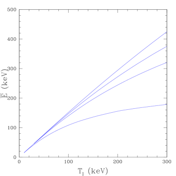
Figure 4: Average energy $\bar{E}$ to which the $\alpha$ particle relaxes as a function of the ion temperature $T_{\rm\scriptscriptstyle I}$ for various electron temperatures $T_{e}$. The ascending curves describing larger values of $\bar{E}$ have the increasing electron temperatures $T_{e}=10\,,\,30\,,\,50\,,\,100$ keV. When $T_{e}=T_{\rm\scriptscriptstyle I}=T$ then $\bar{E}=\frac{3}{2}\,T$. The background plasma is equimolar DT with electron number density $n_{e}=1.0\times 10^{25}\,{\rm cm^{-3}}$.

III Formal Solution

III.1 A Homogeneous and Isotropic Source

We shall assume that the background plasma parameters, such as its density and temperatures, change very little over distances that are large in comparison with the stopping distance of the charged impurity particles, and that the plasma parameters also change very little during the stopping time. Thus the plasma is treated as homogeneous and static. In addition, we assume that the sources of the impurity particles are distributed uniformly in space and that they emit the impurity particles isotropically with a definite energy $E_{0}$. For example, the fusion process in a homogeneous DT plasma produces $\alpha$ particles uniformly in space and isotropically in angle with an initial energy of $E_{0}=3.54$ MeV. Thus, instead of considering the motion of a single test particle, we compute energy partitions and final states of charged particles emitted isotropically with a definite energy $E_{0}$ from a uniform distribution of sources. This greatly simplifies the problem in that we can employ the homogeneous Fokker-Planck Eq. (31) except that it is now modified to include a time-varying source of particles of energy $E_{0}$:

$$\left\{\frac{\partial}{\partial t}-\frac{2}{mv}\,\frac{\partial}{\partial E}\,E\left[{\cal A}(E)+\langle T{\cal A}(E)\rangle\,\frac{\partial}{\partial E}\right]\right\}\,f(E,t)=\delta\left(E-E_{0}\right)\,s(t)\,.$$ (40)

The number and energy densities, $n(t)$ and ${\cal E}(t)$, are simply given by removing the spatial volume integrations from the previous definitions (12) and (13). The inhomogeneous Fokker-Planck equation (40) gives the time variations of these quantities:

$$\dot{n}(t)=\int\frac{d^{3}p}{(2\pi\hbar)}\,\delta\left(E-E_{0}\right)\,s(t)=\frac{s(t)}{2\pi^{2}\hbar^{3}}\,\sqrt{2m^{3}E_{0}}\,,$$ (41)

and

$$\dot{\cal E}(t) = E_{0}\,\dot{n}(t)-\int\frac{d^{3}{\bf p}}{(2\pi\hbar)^{3}}\,v\,\left\{\left[{\cal A}_{\rm\scriptscriptstyle I}(E)+{\cal A}_{e}(E)\right]+\left[T_{\rm\scriptscriptstyle I}\,{\cal A}_{\rm\scriptscriptstyle I}(E)+T_{e}\,{\cal A}_{e}(E)\right]\frac{\partial}{\partial E}\right\}\,f(E,t)\,.$$

When the impurity source $s(t)$ is turned on and then attains a constant fixed value $s_{0}$, the number density $n(t)$ eventually increases linearly in time,

$$n(t) = \int_{-\infty}^{t}dt^{\prime}\,\dot{n}(t^{\prime})=\frac{\sqrt{2m^{3}E_{0}}}{2\pi^{2}\hbar^{3}}\,\int_{-\infty}^{t}dt^{\prime}\,s(t^{\prime})$$ (43)

$$= \dot{n}_{\infty}\,t+{\rm constant}\,,$$

where

$$\dot{n}_{\infty}=\frac{s_{0}}{2\pi^{2}\hbar^{3}}\,\sqrt{2m^{3}E_{0}}\,.$$ (44)

III.2 Asymptotic Solution to the Inhomogeneous Problem

We turn now to obtain the asymptotic solution to (40) satisfying the initial condition that there are no impurity particles in the distant past.

As a first step in obtaining the asymptotic solution of the inhomogeneous Fokker-Planck equation (40), we set

$$f(E,t)=\exp\left\{-S(E)/2\right\}\,g(E,t)\,.$$ (45)

Multiplying the resulting Fokker-Planck equation by $\exp\{S(E)/2\}$ on the left yields a similarity transformation that converts the (velocity $\sim$ momentum) differential operator structure in Eq. (40) into

$$H=-\left[\frac{\partial}{\partial{\bf p}}\cdot\hat{\bf v}-\frac{v{\cal A}(E)}{2\langle T{\cal A}(E)\rangle}\right]\,\frac{\langle T{\cal A}(E)\rangle}{v}\,\left[\hat{\bf v}\cdot\frac{\partial}{\partial{\bf p}}+\frac{v{\cal A}(E)}{2\langle T{\cal A}(E)\rangle}\right]\,,$$ (46)

so that the new Fokker-Planck equation now appears as

$$\left\{\frac{\partial}{\partial t}+H\right\}g(E,t)=\delta\left(E-E_{0}\right)e^{S(E_{0})/2}\,s(t)\,.$$ (47)

Incorporating the boundary condition that the solution vanishes initially, the inhomogeneous differential equation (47) has a formal solution:

$$g(E,t)=\int_{-\infty}^{t}dt^{\prime}\,e^{-H(t-t^{\prime})}\,\delta\left(E-E_{0}\right)\,e^{S(E_{0})/2}\,s(t^{\prime})\,.$$ (48)

Because of the operator nature of the formal solution (48), it is convenient to view functions in momentum space as vectors in an abstract real vector space and define an inner product by

$$(\psi,\chi)=\int\frac{d^{3}{\bf p}}{(2\pi\hbar)^{3}}\,\psi({\bf p})\,\chi({\bf p})\,.$$ (49)

With obvious partial integrations, it is straightforward to verify that $H$ considered as an operator on this function space is Hermitian with this definition of the inner product.

In view of our previous work, it is easy to check that

$$\phi({\bf p})={\cal N}^{1/2}\,\exp\left\{-S(E)/2\right\}$$ (50)

now appears as a zero mode of the operator $H$,

$$H\,\phi=0$$ (51)

that has unit normalization,

$$(\phi,\phi)=1\,.$$ (52)

Except for this zero mode function, the remaining spectrum of $H$ is positive. This is true because, for any function $\psi({\bf p})$,

$$(\psi,H\psi)=\int\frac{d^{3}{\bf p}}{(2\pi\hbar)^{3}}\,\frac{\langle T{\cal A}(E)\rangle}{v}\left\{\left[\hat{\bf v}\cdot\frac{\partial}{\partial{\bf p}}+\frac{v\,{\cal A}(E)}{2\langle T{\cal A}(E)\rangle}\right]\psi({\bf p})\right\}^{2}\geq 0\,,$$ (53)

since an examination of our results for the ${\cal A}$ coefficients shows that $\langle T{\cal A}(E)\rangle\geq 0$. The equality in Eq. (53) holds only if

$$\left[\hat{\bf v}\cdot\frac{\partial}{\partial{\bf p}}+\frac{v\,{\cal A}(E)}{2\langle{T\cal A}(E)\rangle}\right]\psi({\bf p})=0\,.$$ (54)

The spherically symmetric solution $\psi({\bf p})=\psi(|{\bf p}|)$ is clearly the previous zero mode function $\psi({\bf p})=\phi(E)$. Hence within the class of isotropic solutions — the only class that is relevant to our work — there are no other zero modes of $H$ and all its other eigenvalues are positive. Since the operator $H$ is Hermitian,

$$\phi\,H=0\,.$$ (55)

In view of this adjoint equation, it follows that

$$\phi\,e^{-H(t-t^{\prime})}=1\,,$$ (56)

as one easily verifies by taking the time derivative.

Except for this zero mode, we have shown that the other eigenvalues of the Hermitian operator $H$ are positive. This positivity constraint must be obeyed, for otherwise the Fokker-Planck would have diverging “runaway” solutions at large times. The operator that projects out the zero mode is obviously the outer product of the zero mode vector with itself,

$$P=\phi\otimes\phi\,,$$ (57)

and we write the complement operator as

$$Q=1-P\ ,$$ (58)

where the first term in (58) is the unit operator on the function space. By definition, the operator $P$ acts on an arbitrary function $\psi$ as

$$P\,\psi({\bf p})=\Big{(}\phi\otimes\phi\Big{)}\psi({\bf p})=\phi({\bf p})\,(\phi,\psi)\ .$$ (59)

We now see that the unit operator in the form $P+Q$ acting on $g(E,t)$ in (48) produces

$$g(E,t) = \phi({\bf p})\,\int\frac{d^{3}p^{\prime}}{(2\pi\hbar)^{3}}\,\phi({\bf p}^{\prime})\delta\left(E^{\prime}-E_{0}\right)\,e^{S(E_{0})/2}\,\int_{-\infty}^{t}dt^{\prime}\,s(t^{\prime})$$ (60)

$$\qquad+\int_{-\infty}^{t}dt^{\prime}\,e^{-H(t-t^{\prime})}\,Q\delta\left(E-E_{0}\right)\,e^{S(E_{0})/2}\,s(t^{\prime})\,.$$

The momentum integral in the first term of (60) is easy to evaluate,

$$\phi({\bf p})\,\int\frac{d^{3}{\bf p}^{\prime}}{(2\pi\hbar)^{3}}\,\phi({\bf p}^{\prime})\delta\left(E^{\prime}-E_{0}\right)\,e^{S(E_{0})/2}={\cal N}\,e^{-S(E)/2}\,\frac{\sqrt{2m^{3}E_{0}}}{2\pi^{2}\hbar^{3}}\,.$$ (61)

As for the second term, since the operator $Q$ selects out the positive eigenvalues of $H$, an integration by parts can be performed to produce

$$\int_{-\infty}^{t}dt^{\prime}\,e^{-H(t-t^{\prime})}\,Q\delta\left(E-E_{0}\right)\,e^{S(E_{0})/2}\,s(t^{\prime}) = \frac{1}{H}\,Q\delta\left(E-E_{0}\right)\,e^{S(E_{0})/2}\,s(t)$$

$$- \!\!\!\!\!\!\!\!\!\int_{-\infty}^{t}dt^{\prime}\,e^{-H(t-t^{\prime})}\,\frac{1}{H}\,Q\delta\left(E-E_{0}\right)\,e^{S(E_{0})/2}\,\dot{s}(t^{\prime})\,.$$

We now assume that the source $s(t)$ is adiabatically turned on and attains the constant value $s(t)=s_{0}$ at late times. In the asymptotic limit, the rate $\dot{s}(t)$ is therefore vanishingly small and the second term in Eq. (LABEL:Pong) may be neglected. We may also replace $s(t)$ by its asymptotic value $s_{0}$ in the first line. Hence, upon multiplying $g(E,t)$ by $\exp\{-S(E)/2\}$ to return to the function $f(E,t)$, we obtain

$$f(E,t)={\cal N}\,e^{-S(E)}\,\frac{\sqrt{2m^{3}E_{0}}}{2\pi^{2}\hbar^{3}}\,\int_{-\infty}^{t}dt^{\prime}\,s(t^{\prime})+\bar{f}(E)\,,$$ (63)

where

$$\bar{f}(E)=e^{-S(E)/2}\,\frac{1}{H}\,Q\delta\left(E-E_{0}\right)\,e^{S(E_{0})/2}\,s_{0}\,.$$ (64)

Upon integrating (41), we can write this asymptotic late time solution more suggestively as

$$f(E,t)=n(t)f_{\infty}(E)+\bar{f}(E)\,,$$ (65)

with $f_{\infty}(E)={\cal N}\,e^{-S(E)}$. We emphasize that expression (65) is the asymptotic late-time solution to the inhomogeneous Fokker-Planck equation since the term involving the derivative $\dot{s}(t)$ is omitted.

III.3 Energy Deposition

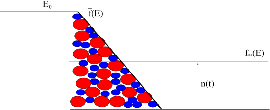
Figure 5: The waterfall analogy: the small blue rocks represent the plasma electrons while the larger red rocks are the plasma ions. The motion of the ‘water’ represents the evolution of the impurity ions that are injected into the background plasma. As ‘water’ falls down the electron-ion slope at a constant rate determined by $\bar{f}(E)$, energy is deposited into electrons and ions. At the bottom of the fall is a lake into which the excess ‘water’ drains and whose height $n(t)$ rises linearly with time.

Before presenting an explicit version of the formal solution (65), we pause to describe its physical interpretation and its relation to the ways in which the stopping charged particle deposits its energy to the background plasma. At large times, the phase-space density has the time-independent contribution $f_{\infty}(E)={\cal N}\,\exp\{-S(E)\}$ into which any set of initial test particles must relax, and the first term of (65) describes this distribution normalized to the correct density $n(t)$. There remains a time-independent part $\bar{f}(E)$ that describes the stationary process of particles losing energy to the background electrons and ions as particles pass through “energy bins” from the initial energy $E_{0}$ to the final asymptotic distribution. The situation described here can be pictured as the flow of water over a rocky waterfall that slows the motion of the water as it descends. The initial rate of flow of the river corresponds to the rate $\dot{n}(t)$; the height $h$ of the waterfall giving a potential energy proportional to $gh$ corresponds to the initial energy $E_{0}$. The energy dissipated in the fall corresponds to the energies lost to the ions and electrons. The final flow into a horizontal lake corresponds to the build up of the particles in their final distribution described by $f_{\infty}(E)$. This analogy is depicted in Fig. 5.

III.3.1 Energy Splitting

Upon inserting the form (65) into Eq. (LABEL:Edot), we can identify the asymptotic constant rates of energy loss as

$$\bar{E}\,\dot{n}_{\infty}=\left[E_{0}-E_{\rm\scriptscriptstyle I}-E_{e}\right]\,\dot{n}_{\infty}\,,$$ (66)

in which

$$\frac{E_{\rm\scriptscriptstyle I}}{E_{0}} = \frac{1}{\dot{n}_{\infty}\,E_{0}}\int\frac{d^{3}{\bf p}}{(2\pi\hbar)^{3}}\,v\,{\cal A}_{\rm\scriptscriptstyle I}(v)\,\left[1+T_{\rm\scriptscriptstyle I}\,\frac{\partial}{\partial E}\right]\,\bar{f}(E)\,,$$ (67)

and

$$\frac{E_{e}}{E_{0}} = \frac{1}{\dot{n}_{\infty}\,E_{0}}\int\frac{d^{3}{\bf p}}{(2\pi\hbar)^{3}}\,v\ {\cal A}_{e}(v)\,\left[1+T_{e}\,\frac{\partial}{\partial E}\right]\,\bar{f}(E)\,.$$ (68)

Thus Eqs. (67) and (68) are the constant fractions of the original energy $E_{0}$ deposited into ionic energy $E_{\rm\scriptscriptstyle I}$ and electronic energy $E_{e}$ — the energy losses analogous to those of the water passing through the rocky waterfall.

III.3.2 Plasma Heating and Energy Exchange

exchange

The original energy goes into energies lost to the ions and electrons, with the remainder the average final energy $\bar{E}$ of an impurity particle. For a background plasma with the ions and electrons at a common temperature $T$, $\bar{E}=3T/2$, and the result (66) becomes obvious.

When the electrons and ions have the same temperature $T=T_{e}=T_{\rm\scriptscriptstyle I}$, the slowing down of fast particles in the plasma gives a steady-state heating rate per unit volume ${\cal P}=[E_{\rm\scriptscriptstyle I}+E_{e}]\,\dot{n}_{\infty}$. This heating raises the temperature $T$ of the plasma, but in most cases, the rate of this heating is small in comparison with the slowing down time of the fast impurity particles, and so our quasi-steady-state computation is valid, with the temperature treated as a slowing varying function in our formulae.

When the electrons and ions have different temperatures $T_{e}$ and $T_{\rm\scriptscriptstyle I}$, the situation may be quite different. In addition to the overall plasma heating ${\cal P}$, the final ensemble of the impurity particles works to bring the electrons and ions to a common temperature. Returning to Eq. (LABEL:Edot), we see that the final ensemble contribution produces energy density transfer rates to the ions and electrons given by

$$\dot{\cal E}_{\rm\scriptscriptstyle I}(t) = +\int\frac{d^{3}{\bf p}}{(2\pi\hbar)^{3}}\,v\,{\cal A}_{\rm\scriptscriptstyle I}(v)\left[1+T_{\rm\scriptscriptstyle I}\,\frac{\partial}{\partial E}\right]\,{\cal N}\,\exp\left\{-S(E)\right\}\,n(t)\,,$$ (69)

and

$$\dot{\cal E}_{e}(t) = +\int\frac{d^{3}{\bf p}}{(2\pi\hbar)^{3}}\,v\,{\cal A}_{e}(v)\left[1+T_{e}\,\frac{\partial}{\partial E}\right]\,{\cal N}\,\exp\left\{-S(E)\right\}\,n(t)\,.$$ (70)

Carrying out the energy derivatives yields

$$\dot{\cal E}_{\rm\scriptscriptstyle I}(t) = -\left(T_{\rm\scriptscriptstyle I}-T_{e}\right)\,C^{\alpha}_{{\rm\scriptscriptstyle I}\,e}\,,$$ (71)

and

$$\dot{\cal E}_{e}(t) = -\left(T_{e}-T_{\rm\scriptscriptstyle I}\right)\,C^{\alpha}_{e\,{\rm\scriptscriptstyle I}}\,,$$ (72)

where

$$C^{\alpha}_{{\rm\scriptscriptstyle I}\,e}=C^{\alpha}_{e\,{\rm\scriptscriptstyle I}} = n(t)\,\int\frac{d^{3}{\bf p}}{(2\pi\hbar)^{3}}\,v\,\frac{{\cal A}_{\rm\scriptscriptstyle I}(v)\,{\cal A}_{e}(v)}{\langle T{\cal A}\rangle}\,{\cal N}\,\exp\left\{-S(E)\right\}\,.$$ (73)

Since

$$\dot{\cal E}_{\rm\scriptscriptstyle I}(t)+\dot{\cal E}_{e}(t)=0\,,$$ (74)

there is no net heating of the plasma. This process only brings the ions and electrons to a common temperature.

In the absence of the impurity particle quasi-static equilibrium ensemble, the thermal relaxation rate coefficients are well approximated by

$$C_{{\rm\scriptscriptstyle I}\,e}=C_{e\,{\rm\scriptscriptstyle I}}=\frac{\kappa_{e}^{2}}{2\pi}\,\omega_{\rm\scriptscriptstyle I}^{2}\sqrt{\frac{m_{e}}{2\pi\,T_{e}}}\,\frac{1}{2}\left\{\ln\left(\frac{8T_{e}^{2}}{\hbar^{2}\,\omega_{e}^{2}}\right)-\gamma-1\right\}\,.$$ (75)

Here

$$\kappa_{e}^{2}=\frac{e^{2}\,n_{e}}{T_{e}}$$ (76)

is the squared electron Debye wave number, and

$$\omega_{a}^{2}=\frac{e_{a}^{2}n_{a}}{m_{a}}$$ (77)

is the definition of the squared plasma frequency for particle $a$, with the electron squared plasma frequency $\omega_{e}^{2}$ specified by $a=e$, while the total squared ionic plasma frequency $\omega_{\rm\scriptscriptstyle I}^{2}$ is the sum over all the ions in the plasma

$$\omega_{\rm\scriptscriptstyle I}^{2}={\sum}_{i}\,\omega_{i}^{2}\,.$$ (78)

In numerical terms, for an equimolar DT plasma,

$$C_{{\rm\scriptscriptstyle I}\,e}=3.13\times 10^{-26}\,n_{e}^{2}\,T_{e}^{-3/2}\,\left\{\ln\left(5.80\times 10^{27}\,\frac{T_{e}^{2}}{n_{e}}\right)\ -1.58\right\}\,{\rm cm}^{-3}\,{\rm ps}^{-1}\,,$$ (79)

in which the electron density $n_{e}$ is measured in ${\rm cm}^{-3}$, the electron temperature $T_{e}$ in keV, and the overall units are $(1.0\,{\rm cm}^{-3})/(1.0\times 10^{-12}\,{\rm sec})$ as indicated.

The total rate coefficient for electron-ion thermal relaxation is the sum $C_{{\rm\scriptscriptstyle I}\,e}+C^{\alpha}_{{\rm\scriptscriptstyle I}\,e}$. It is of interest to compare $C^{\alpha}_{{\rm\scriptscriptstyle I}\,e}$ to $C_{{\rm\scriptscriptstyle I}\,e}$. Since $C^{\alpha}_{{\rm\scriptscriptstyle I}\,e}$ is proportional to the number of impurity particles that come into their final equilibrium state $n(t)$, this comparison can be made independent of this density by evaluating the ratio of $C^{\alpha}_{{\rm\scriptscriptstyle I}\,e}/n(t)$ to $C_{{\rm\scriptscriptstyle I}\,e}/n_{\rm\scriptscriptstyle I}$. In Fig. 6 we plot this dimensionless ratio as a function of the electron temperature $T_{e}$ for various values of the ion temperature $T_{\rm\scriptscriptstyle I}$ ranging from 3 keV to 100 keV at an electron density $n_{e}=1.0\times 10^{24}\,{\rm cm}^{-3}$. Explicit calculation shows that the dependence of this ratio upon the electron density $n_{e}$ is weak. As $n_{e}$ is increased from $1.0\times 10^{24}\,{\rm cm}^{-3}$ to $1.0\times 10^{26}\,{\rm cm}^{-3}$, the greatest change in the ratio occurs for $T_{\rm\scriptscriptstyle I}\gg T_{e}$ : for $T_{\rm\scriptscriptstyle I}=100$ keV and $T_{e}=3$ keV, the ratio increases by 20%.

We must add the caveat, already noted in the Introduction, that the discussion that we have just made applies only to the case in which the final alpha particle population is not large. Hence, although in some cases the ratios shown in Fig. 6 are of order one, the net effect of this new mechanism must be relatively small.

Figure 6: The ratio $n_{\rm\scriptscriptstyle I}\,C^{\alpha}_{{\rm\scriptscriptstyle I}\,e}/n\,C_{{\rm\scriptscriptstyle I}\,e}$ as a function of the electron temperature for an equimolar DT plasma with an electron density of $1.0\times 10^{24}\,{\rm cm}^{-3}$ for ion temperatures of 3 keV (blue), 10 keV (red), 30 keV (black), and 100 keV (green).

III.4 Results in Terms of $dE/dx$

The results (67), (68), (69), and (70) all have the generic structure

$$\tilde{E}_{{\rm\scriptscriptstyle I},e} = \int\frac{d^{3}{\bf p}}{(2\pi\hbar)^{3}}\,v\ {\cal A}_{{\rm\scriptscriptstyle I},e}(v)\,\left[1+T_{{\rm\scriptscriptstyle I},e}\,\frac{\partial}{\partial E}\right]\,\tilde{f}(E)\,.$$ (80)

Here we may write

$$\frac{\partial}{\partial E}\,\tilde{f}(E)=\frac{1}{2E}\,{\bf p}\cdot\frac{\partial}{\partial{\bf p}}\tilde{f}(E)\,,$$ (81)

use ${\bf p}=m{\bf v}$, and integrate by parts to obtain

$$\tilde{E}_{{\rm\scriptscriptstyle I},e} = \int\frac{d^{3}{\bf p}}{(2\pi\hbar)^{3}}\,\tilde{f}(E)\,\left[v-\frac{T_{{\rm\scriptscriptstyle I},e}}{m}\,\frac{\partial}{\partial{\bf v}}\cdot\hat{\bf v}\right]{\cal A}_{{\rm\scriptscriptstyle I},e}(v)\,.$$ (82)

As remarked in the Introduction [Eq. (6)], the expression to the right of $\tilde{f}(E)$ in the integrand above is just $v\,dE_{{\rm\scriptscriptstyle I},e}(E)/dx$. The integrand does not depend upon the direction of ${\bf p}$. Thus the angular integration simply provides a factor of $4\pi$. Using $vdp=dE$, we now have

$$\tilde{E}_{{\rm\scriptscriptstyle I},e} = \int_{0}^{\infty}dE\,\frac{dE_{{\rm\scriptscriptstyle I},e}(E)}{dx}\,\frac{p^{2}}{2\pi^{2}\hbar^{3}}\,\tilde{f}(E)\,.$$ (83)

Thus all of our results involve a factor of the stopping power $dE_{{\rm\scriptscriptstyle I},e}/dx$ for the ions or for the electrons, but the integration weight involves a more subtle function than those in the naive formulae (1) and (2) given in the Introduction.

IV Explicit Solution

IV.1 General Development

We turn now to the explicit construction of the function $\bar{f}(E)$ from the formal expression (64). We start by multiplying Eq. (64) by the (velocity $\sim$ momentum) differential operator structure in Eq. (40). Passing this operator through the factor $\exp\{-S(E)/2\}$ is equivalent to the similarity transformation that converts it into the operator $H$. Hence,

$$-\frac{\partial}{\partial{\bf p}}\cdot\hat{\bf v}\,\left[{\cal A}+\langle T{\cal A}(E)\rangle\,\frac{\hat{\bf v}}{v}\cdot\frac{\partial}{\partial{\bf p}}\right]\,\bar{f}(E)=e^{-S(E)/2}\,Q\,e^{+S(E)/2}\,\delta\left(E-E_{0}\right)\,s_{0}\,,$$ (84)

and remembering Eqs. (28), we see that this is equivalent to

$$-\frac{\partial}{\partial v}\,\frac{v^{2}}{m}\left[{\cal A}+\langle T{\cal A}(E)\rangle\,\frac{\partial}{\partial E}\right]\,\bar{f}(E) = v^{2}e^{-S(E)/2}\,Q\,e^{+S(E)/2}\,\delta\left(E-E_{0}\right)\,s_{0}$$

$$= \delta\left(E-E_{0}\right)\,\frac{2E_{0}}{m}\,s_{0}-v^{2}{\cal N}\,e^{-S(E)}\,\frac{\sqrt{2m^{3}E_{0}}}{2\pi^{2}\hbar^{3}}\,s_{0}\,.$$

In the second equality we employed the definitions (57) and (58) of the operators $P$ and $Q$ and in the last line used the result (61). Obviously, a trivial first integral of this differential equation exists. Since the constant of integration must be chosen to make $\bar{f}(E)$ vanish at large $E$, this first integral reads

$$\left[{\cal A}(E)+\langle T{\cal A}(E)\rangle\frac{\partial}{\partial E}\right]\bar{f}(E) = \frac{s_{0}}{E}\sqrt{\frac{mE_{0}}{2}}\left\{\theta\left(E_{0}-E\right)-\int_{E}^{\infty}dE^{\prime}\,\frac{m\,\sqrt{2mE^{\prime}}}{2\pi^{2}\hbar^{3}}\,{\cal N}e^{-S(E^{\prime})}\right\},$$

where $\theta(x)$ is the unit step function that vanishes for $x<0$. Note that, in view of the normalization (33),

$$\int_{0}^{\infty}dE^{\prime}\frac{m\,\sqrt{2mE^{\prime}}}{2\pi^{2}\hbar^{3}}\,{\cal N}\,e^{-S(E^{\prime})}=\int\frac{d^{3}{\bf p}^{\prime}}{(2\pi\hbar)^{3}}\,{\cal N}\,e^{-S(E^{\prime})}=1\,,$$ (87)

and so the sum of the terms in the curly braces in Eq. (LABEL:ffbarrr) vanishes when $E\to 0$. This is in accord with the fact that these terms on the right of Eq. (LABEL:ffbarrr) were produced by the integral of a derivative on the left-hand side of Eq. (LABEL:ffbarr), a derivative of a quantity that vanishes at both $E=0$ and $E=\infty$. Moreover, since the curly braces vanishes at $E=0$, the right-hand side of Eq. (LABEL:ffbarrr) is finite at this end point as it must be.

At this juncture, it is convenient to remember the definition (44) of $\dot{n}_{\infty}$, which can be expressed as

$$\sqrt{\frac{mE_{0}}{2}}\,s_{0}=\frac{\pi^{2}\hbar^{3}}{mE_{0}}\,E_{0}\,\dot{n}_{\infty}\,,$$ (88)

and to simplify the notation by writing

$$\overline{\cal N}=\frac{m\,\sqrt{2m}}{2\pi^{2}\hbar^{3}}\,{\cal N}\,,$$ (89)

so that we have

$$\int_{0}^{\infty}dE^{\prime}\sqrt{E^{\prime}}\,\,\overline{\cal N}\,\,e^{-S(E^{\prime})}=1\,.$$ (90)

Thus, Eq.(LABEL:ffbarrr) now reads:

$$\left[{\cal A}(E)+\langle T{\cal A}(E)\rangle\frac{\partial}{\partial E}\right]\,\frac{\bar{f}(E)}{E_{0}\,\dot{n}_{\infty}} = \frac{\pi^{2}\hbar^{3}}{mE_{0}E}\,\left\{\theta\left(E_{0}-E\right)\,-\int_{E}^{\infty}dE^{\prime}\sqrt{E^{\prime}}\,\overline{\cal N}\,e^{-S(E^{\prime})}\right\}\,.$$

To solve this differential equation, we set

$$\bar{f}(E)=e^{-S(E)}\,\bar{g}(E)\,,$$ (92)

because then

$$\left[{\cal A}(E)+\langle T{\cal A}(E)\rangle\frac{\partial}{\partial E}\right]\,\bar{f}(E)=e^{-S(E)}\,\langle T{\cal A}(E)\rangle\,\frac{\partial}{\partial E}\,\bar{g}(E)\,.$$ (93)

Since the integrating factor involves $\exp\{+S(E)\}$, which exponentially increases without bound as the energy increases, to obtain a finite well-defined result we must integrate over the range $E^{\prime}=0$ to $E^{\prime}=E$ and obtain

$$\frac{\bar{g}(E)}{E_{0}\,\dot{n}_{\infty}} = \frac{\pi^{2}\hbar^{3}}{mE_{0}}\,\int_{0}^{E}\frac{dE^{\prime}}{E^{\prime}}\,\frac{e^{+S(E^{\prime})}}{\langle T{\cal A}(E^{\prime})\rangle}\,\left\{\theta\left(E_{0}-E^{\prime}\right)\,-\int_{E^{\prime}}^{\infty}dE^{\prime\prime}\sqrt{E^{\prime\prime}}\,\,\overline{{\cal N}}\,\,e^{-S(E^{\prime\prime})}\right\}.$$ (94)

IV.2 Energy Fractions and $dE/dx$

The customary expressions for the energy fractions in terms of the stopping power [Eqs. (1) and (2)] emerge for low temperatures. To see this, we note that in this case, the energy integration range is very large on the scale of the temperature, and that the work of Appendix B shows that the electron contribution dominates over most of this range so that we may approximate

$$S(E)\simeq\frac{E}{T_{e}}\,.$$ (95)

Moreover, the sum rule (90) implies that the terms in the curly braces in Eq. (94) cancel when $E^{\prime}\simeq\tilde{E}$, where $\tilde{E}$ is a lower energy limit that is on the order of the electron temperature $T_{e}$. On the other hand, the integral in the curly braces in Eq. (94) is exponentially small when the integration variable $E^{\prime}$ is somewhat larger that the electron temperature $T_{e}$. Hence, in the low temperature case, Eqs. (92) and (94) provide the approximate solution

$$\bar{f}(E) \simeq \dot{n}_{\infty}\,\frac{\pi^{2}\hbar^{3}}{m}\,\int_{0}^{E}\frac{dE^{\prime}}{E^{\prime}}\,\exp\left\{-\frac{1}{T_{e}}\,\left(E-E^{\prime}\right)\right\}\,\frac{1}{\langle T{\cal A}(E^{\prime})\rangle}\,\theta\Big{(}E_{0}-E^{\prime}\Big{)}\,\theta\Big{(}E^{\prime}-\tilde{E}\Big{)}\,.$$

Repeatedly using

$$\exp\left\{-\frac{1}{T_{e}}\,\left(E-E^{\prime}\right)\right\}=T_{e}\,\frac{d}{dE^{\prime}}\,\exp\left\{-\frac{1}{T_{e}}\,\left(E-E^{\prime}\right)\right\}\,,$$ (97)

and repeatedly integrating by parts, shows that the leading term in the low temperature case is given by the upper-limit contribution of the first term in this sequence:

$$f(E) \simeq \dot{n}_{\infty}\,\frac{\pi^{2}\hbar^{3}}{m}\,\frac{T_{e}}{E}\,\frac{1}{\langle T{\cal A}(E)\rangle}\,\theta\Big{(}E_{0}-E\Big{)}\,\theta\Big{(}E-\tilde{E}\Big{)}\,.$$ (98)

Placing this approximate result in the generic form (83) to evaluate the energy fractions (67) and (68) yields

$$\frac{E_{\rm\scriptscriptstyle I}}{E_{0}}\simeq\int_{\tilde{E}}^{E_{0}}\frac{dE}{E_{0}}\,\frac{T_{e}}{\langle T{\cal A}(E)\rangle}\,\frac{dE_{\rm\scriptscriptstyle I}}{dx}(E)\,,$$ (99)

and

$$\frac{E_{e}}{E_{0}}\simeq\int_{\tilde{E}}^{E_{0}}\frac{dE}{E_{0}}\,\frac{T_{e}}{\langle T{\cal A}(E)\rangle}\,\frac{dE_{e}}{dx}(E)\,.$$ (100)

In the low temperature case, the generic relation (6) gives $dE/dx\simeq{\cal A}$ and so

$$\frac{T_{e}}{\langle T{\cal A}(E)\rangle}\simeq\frac{T_{e}}{T_{\rm\scriptscriptstyle I}\,dE_{\rm\scriptscriptstyle I}/dx(E)+T_{e}\,dE_{e}/dx(E)}\,.$$ (101)

In the equal temperature case,

$$\frac{T_{e}}{\langle T{\cal A}(E)\rangle}\to\frac{1}{dE/dx(E)}\,,$$ (102)

and, setting $E_{0}\to 0$, the low temperature expressions (99) and (100) reduce to the commonly used Eqs. (1) and (2) discussed in the Introduction.

IV.3 Equal Electron and Ion Temperatures

The case in which the ions and electrons have the same temperature, $T_{\rm\scriptscriptstyle I}=T_{e}=T$, is simple in several respects. First of all, it is physically simpler because the final distribution of the stopping charged particles is the Maxwell-Boltzmann thermal equilibrium distribution of the background plasma,

$$\exp\left\{-S(E)\right\}=\exp\left\{-\frac{E}{T}\right\}\,.$$ (103)

Thus, the energy transfer processes (69) and (70) do not appear because, with Eq. (103) holding, the combinations in the square brackets in these equations annihilate $\exp\{-S(E)\}$. Thus, only the energy partitions $E_{\rm\scriptscriptstyle I}$ and $E_{e}$ need to be examined, and these obey the obvious sum rule

$$\frac{3}{2}\,T=E_{0}-E_{\rm\scriptscriptstyle I}-E_{e}\,,$$ (104)

to which Eq. (66) reduces. Secondly, it is mathematically simpler because there is no need to find an explicit solution to Eq. (94) because Eq. (LABEL:fffbarrr) reduces to

$$\left[1+T\,\frac{\partial}{\partial E}\right]\,\frac{\bar{f}(E)}{E_{0}\dot{n}_{\infty}} = \theta\left(E_{0}-E\right)\,\frac{1}{E{\cal A}(E)}\,\frac{\pi^{2}\hbar^{3}}{mE_{0}}$$ (105)

$$-\frac{1}{E_{0}E\,{\cal A}(E)}\,\left(\frac{2\pi\hbar^{2}}{mT}\right)^{3/2}\,\int_{E}^{\infty}dE^{\prime}\,\sqrt{2mE^{\prime}}\,e^{-\beta E^{\prime}}\,.$$

The operation in the square brackets that acts on $\bar{f}(E)$ on the left-hand side of this equation is just that which appears in the energy partitions (67) and (68).

Placing this expression into the energy partitions Eqs. (67) and (68) and changing the momentum integration into an integration over energy expresses the fractional energy loss into ions and electrons as

$$\frac{E_{\rm\scriptscriptstyle I}}{E_{0}} = \int_{0}^{E_{0}}\frac{dE}{E_{0}}\,\frac{{\cal A}_{\rm\scriptscriptstyle I}(E)}{{\cal A}(E)}-\int_{0}^{\infty}\frac{dE}{E_{0}}\,\frac{{\cal A}_{\rm\scriptscriptstyle I}(E)}{{\cal A}(E)}\,\frac{2\,\beta^{3/2}}{\sqrt{\pi}}\,\int_{E}^{\infty}dE^{\prime}\,\sqrt{E^{\prime}}\,e^{-\beta E^{\prime}}$$ (106)

and

$$\frac{E_{e}}{E_{0}} = \int_{0}^{E_{0}}\frac{dE}{E_{0}}\,\frac{{\cal A}_{e}(E)}{{\cal A}(E)}-\int_{0}^{\infty}\frac{dE}{E_{0}}\,\frac{{\cal A}_{e}(E)}{{\cal A}(E)}\,\frac{2\,\beta^{3/2}}{\sqrt{\pi}}\,\int_{E}^{\infty}dE^{\prime}\,\sqrt{E^{\prime}}\,e^{-\beta E^{\prime}}\,,$$ (107)

where $\beta=1/T$. Adding these equations gives

$$\left[E_{\rm\scriptscriptstyle I}+E_{e}\right] = E_{0}-\int_{0}^{\infty}dE\,\,\frac{2\,\beta^{3/2}}{\sqrt{\pi}}\,\int_{E}^{\infty}dE^{\prime}\,\sqrt{E^{\prime}}\,e^{-\beta E^{\prime}}$$ (108)

$$= E_{0}-\frac{2\,\beta^{3/2}}{\sqrt{\pi}}\,\int_{0}^{\infty}dE^{\prime}\,{E^{\prime}}^{3/2}\,e^{-\beta E^{\prime}}$$

$$= E_{0}-\frac{3}{2}\,T\,,$$

where the second line follows from a partial integration, and the last line from the definition of $\Gamma(5/2)$. This is just the obvious result of energy conservation previously stated in Eq. (66).

The results (106) and (107) can be simplified for their explicit evaluation. Writing these results with a trivial rearrangement of the terms presents them as:

$$\frac{E_{\rm\scriptscriptstyle I}}{E_{0}} = \int_{0}^{E_{0}}\frac{dE}{E_{0}}\,\frac{{\cal A}_{\rm\scriptscriptstyle I}(E)}{{\cal A}(E)}\left[1-\frac{2\,\beta^{3/2}}{\sqrt{\pi}}\,\int_{E}^{\infty}dE^{\prime}\,\sqrt{E^{\prime}}\,e^{-\beta E^{\prime}}\right]$$ (109)

$$\qquad\qquad\qquad-\int_{E_{0}}^{\infty}\frac{dE}{E_{0}}\,\frac{{\cal A}_{\rm\scriptscriptstyle I}(E)}{{\cal A}(E)}\,\frac{2\,\beta^{3/2}}{\sqrt{\pi}}\,\int_{E}^{\infty}dE^{\prime}\,\sqrt{E^{\prime}}\,e^{-\beta E^{\prime}}\,,$$

and

$$\frac{E_{e}}{E_{0}} = \int_{0}^{E_{0}}\frac{dE}{E_{0}}\,\frac{{\cal A}_{e}(E)}{{\cal A}(E)}\left[1-\frac{2\,\beta^{3/2}}{\sqrt{\pi}}\,\int_{E}^{\infty}dE^{\prime}\,\sqrt{E^{\prime}}\,e^{-\beta E^{\prime}}\right]$$ (110)

$$\qquad\qquad\qquad-\int_{E_{0}}^{\infty}\frac{dE}{E_{0}}\,\frac{{\cal A}_{e}(E)}{{\cal A}(E)}\,\frac{2\,\beta^{3/2}}{\sqrt{\pi}}\,\int_{E}^{\infty}dE^{\prime}\,\sqrt{E^{\prime}}\,e^{-\beta E^{\prime}}\,.$$

As we shall see, the second set of double integrals in Eqs. (109) and (110) are exponentially small. Hence it suffices to use the simple bounds

$$\frac{{\cal A}_{\rm\scriptscriptstyle I}(E)}{{\cal A}(E)}=\frac{{\cal A}_{\rm\scriptscriptstyle I}(E)}{{\cal A}_{\rm\scriptscriptstyle I}(E)+{\cal A}_{e}(E)}\leq 1\,,$$ (111)

and similarly

$$\frac{{\cal A}_{e}(E)}{{\cal A}(E)}\leq 1\,.$$ (112)

Using these bounds, we encounter

$$-\int_{E_{0}}^{\infty}\frac{dE}{E_{0}}\,\frac{2\,\beta^{3/2}}{\sqrt{\pi}}\,\int_{E}^{\infty}dE^{\prime}\,\sqrt{E^{\prime}}\,e^{-\beta E^{\prime}} = -\frac{2\,\beta^{3/2}}{\sqrt{\pi}}\,\int_{E_{0}}^{\infty}dE^{\prime}\,\sqrt{E^{\prime}}\,e^{-\beta E^{\prime}}\int_{E_{0}}^{E^{\prime}}\frac{dE}{E_{0}}$$ (113)

$$= -\frac{2\,\beta^{3/2}}{\sqrt{\pi}}\,\int_{E_{0}}^{\infty}dE^{\prime}\,\sqrt{E^{\prime}}\,e^{-\beta E^{\prime}}\left[\frac{E^{\prime}}{E_{0}}-1\right]\,.$$

The variable change $E^{\prime}=E_{0}\,(x+1)$ presents this as

$$-\frac{2\,\beta^{3/2}}{\sqrt{\pi}}\,E_{0}^{3/2}\,e^{-\beta E_{0}}\,\int_{0}^{\infty}dx\,(1+x)^{1/2}\,x\,e^{-\beta E_{0}x}\simeq-\frac{2}{\sqrt{\pi}}\,\frac{1}{\sqrt{\beta E_{0}}}\,e^{-\beta E_{0}}\,,$$ (114)

with the evaluation on the right-hand side following from the fact that $\beta E_{0}\gg 1$ so that only small $x$ regions contribute justifying the replacement $(1+x)^{1/2}\to 1$. Hence we indeed find that the additional double integrals in the energy fractions (109) and (110) are exponentially small, and so with very good accuracy we may write these fractions as

$$\frac{E_{\rm\scriptscriptstyle I}}{E_{0}} = \int_{0}^{E_{0}}\frac{dE}{E_{0}}\,\frac{{\cal A}_{\rm\scriptscriptstyle I}(E)}{{\cal A}(E)}\left[1-\frac{2\,\beta^{3/2}}{\sqrt{\pi}}\,\int_{E}^{\infty}dE^{\prime}\,\sqrt{E^{\prime}}\,e^{-\beta E^{\prime}}\right]\,,$$ (115)

and

$$\frac{E_{e}}{E_{0}} = \int_{0}^{E_{0}}\frac{dE}{E_{0}}\,\frac{{\cal A}_{e}(E)}{{\cal A}(E)}\left[1-\frac{2\,\beta^{3/2}}{\sqrt{\pi}}\,\int_{E}^{\infty}dE^{\prime}\,\sqrt{E^{\prime}}\,e^{-\beta E^{\prime}}\right]\,.$$ (116)

Since

$$\frac{2\,\beta^{3/2}}{\sqrt{\pi}}\,\int_{0}^{\infty}dE^{\prime}\,\sqrt{E^{\prime}}\,e^{-\beta E^{\prime}}=1\,,$$ (117)

we may write

$$1-\frac{2\,\beta^{3/2}}{\sqrt{\pi}}\,\int_{E}^{\infty}dE^{\prime}\,\sqrt{E^{\prime}}\,e^{-\beta E^{\prime}}=\frac{2\,\beta^{3/2}}{\sqrt{\pi}}\,\int_{0}^{E}dE^{\prime}\,\sqrt{E^{\prime}}\,e^{-\beta E^{\prime}}\,,$$ (118)

while partial integration gives

$$\frac{2\,\beta^{3/2}}{\sqrt{\pi}}\,\int_{0}^{E}dE^{\prime}\,\sqrt{E^{\prime}}\,e^{-\beta E^{\prime}}=-\sqrt{\frac{4\beta E}{\pi}}\,e^{-\beta E}+\sqrt{\frac{\beta}{\pi}}\,\int_{0}^{E}dE^{\prime}\,\frac{1}{\sqrt{E^{\prime}}}\,e^{-\beta E^{\prime}}\,.$$ (119)

Hence, using the definition

$${\rm erf}(x)=\frac{2}{\sqrt{\pi}}\,\int_{0}^{x}dy\,e^{-y^{2}}$$ (120)

of the error function, we may write the results (115) and (116) as

$$\frac{E_{\rm\scriptscriptstyle I}}{E_{0}} = \int_{0}^{E_{0}}\frac{dE}{E_{0}}\,\frac{{\cal A}_{\rm\scriptscriptstyle I}(E)}{{\cal A}(E)}\left[{\rm erf}(\sqrt{\beta E})-\sqrt{\frac{4\beta E}{\pi}}\,e^{-\beta E}\right]\,,$$ (121)

and

$$\frac{E_{e}}{E_{0}} = \int_{0}^{E_{0}}\frac{dE}{E_{0}}\,\frac{{\cal A}_{e}(E)}{{\cal A}(E)}\left[{\rm erf}(\sqrt{\beta E})-\sqrt{\frac{4\beta E}{\pi}}\,e^{-\beta E}\right]\,.$$ (122)

These are the results quoted in Eqs. (7) and (8) in the Introduction.

IV.4 Differing Electron and Ion Temperatures

As we have seen, when the ion and electron temperatures of the background plasma differ, $T_{\rm\scriptscriptstyle I}\neq T_{e}$, both the physical interpretation is richer and the mathematics becomes more difficult. With different temperatures, there is the additional physical process in which the final distribution of stopped injected impurity particles works to bring the electrons and ions into thermal equilibrium at a common temperature $T=T_{\rm\scriptscriptstyle I}=T_{e}$. Moreover, mathematically, we must now work with Eq. (94).

We use Eq. (94) to return to the $\bar{f}(E)$ function, and insert the result for $\bar{f}(E)$ into Eqs. (67) and (68) to compute $E_{\rm\scriptscriptstyle I}/E_{0}$ and $E_{e}/E_{0}$. To simplify the resulting formulae, and place them in a form that parallels those for the previous equal ion-electron temperature case we note that

$$\left\{\begin{array}[]{c}{\cal A}_{\rm\scriptscriptstyle I}(E)\\ {\cal A}_{e}(E)\end{array}\right\}\left[1+\left\{\begin{array}[]{c}T_{\rm\scriptscriptstyle I}\\ T_{e}\end{array}\right\}\frac{d}{dE}\right]\,e^{-S(E)}=\left\{\begin{array}[]{c}+\\ -\end{array}\right\}\left[T_{e}-T_{\rm\scriptscriptstyle I}\right]\frac{{\cal A}_{\rm\scriptscriptstyle I}(E){\cal A}_{e}(E)}{\langle T{\cal A}(E)\rangle}\,e^{-S(E)}\,.$$ (129)

Hence, with the definition

$$G(T_{\rm\scriptscriptstyle I},T_{e};E_{0}) = \int_{0}^{\infty}dE\,E\,\frac{{\cal A}_{\rm\scriptscriptstyle I}(E){\cal A}_{e}(E)}{\langle T{\cal A}(E)\rangle}\,e^{-S(E)}$$

$$\!\!\!\!\!\int_{0}^{E}\frac{dE^{\prime}}{E^{\prime}}\,\frac{e^{+S(E^{\prime})}}{\langle T{\cal A}(E^{\prime})\rangle}\,\left\{\theta\left(E_{0}-E^{\prime}\right)\,-\int_{E^{\prime}}^{\infty}dE^{\prime\prime}\sqrt{E^{\prime\prime}}\,\overline{\cal N}\,e^{-S(E^{\prime\prime})}\right\}\,,$$

the energy loss fractions may be expressed as

$$\frac{E_{\rm\scriptscriptstyle I}}{E_{0}} = \left[\frac{T_{e}-T_{\rm\scriptscriptstyle I}}{E_{0}}\right]\,G(T_{\rm\scriptscriptstyle I},T_{e};E_{0})$$

$$+\int_{0}^{\infty}\frac{dE}{E_{0}}\,\frac{T_{\rm\scriptscriptstyle I}\,{\cal A}_{\rm\scriptscriptstyle I}(E)}{\langle T{\cal A}(E^{\prime})\rangle}\,\left\{\theta\left(E_{0}-E\right)\,-\int_{E}^{\infty}dE^{\prime}\sqrt{E^{\prime}}\,\overline{\cal N}\,e^{-S(E^{\prime})}\right\}\,,$$

and

$$\frac{E_{e}}{E_{0}} = \left[\frac{T_{\rm\scriptscriptstyle I}-T_{e}}{E_{0}}\right]\,\,G(T_{\rm\scriptscriptstyle I},T_{e};E_{0})$$

$$+\int_{0}^{\infty}\frac{dE}{E_{0}}\,\frac{T_{e}\,{\cal A}_{e}(E)}{\langle T{\cal A}(E^{\prime})\rangle}\,\left\{\theta\left(E_{0}-E\right)\,-\int_{E}^{\infty}dE^{\prime}\sqrt{E^{\prime}}\,\overline{\cal N}\,e^{-S(E^{\prime})}\right\}\,.$$

The second lines in the results (LABEL:IIIfrac) and (LABEL:eeefrac) are straightforward generalizations of the common ion and electron temperature forms (106) and (107). The first lines of the new results (LABEL:IIIfrac) and (LABEL:eeefrac) cancel when they are summed, so that

$$E_{\rm\scriptscriptstyle I}+E_{e} = +\int_{0}^{E_{0}}dE-\overline{\cal N}\,\int_{0}^{\infty}dE\,\int_{E}^{\infty}dE^{\prime}\,\sqrt{E^{\prime}}\,e^{-S(E^{\prime})}\,.$$ (133)

Upon interchanging integrals,

$$\int_{0}^{\infty}dE\,\int_{E}^{\infty}dE^{\prime}\,\sqrt{E^{\prime}}\,e^{-S(E^{\prime})} = \int_{0}^{\infty}dE\,\sqrt{E}\,e^{-S(E)}\,\int_{0}^{E}dE^{\prime}$$ (134)

$$= \int_{0}^{\infty}dE\,E\,\sqrt{E}\,e^{-S(E)}\,.$$

Hence, on passing from an integration over energy to an equivalent momentum integral and reverting to the corresponding normalization factor ${\cal N}$, we have

$$E_{\rm\scriptscriptstyle I}+E_{e}=E_{0}-\int\frac{d^{3}{\bf p}}{(2\pi\hbar)^{3}}\,E\,{\cal N}\,e^{-S(E)}$$ (135)

or, in view of Eq. (39),

$$E_{\rm\scriptscriptstyle I}+E_{e}=E_{0}-\bar{E}\,,$$ (136)

in which $\bar{E}$ is the average energy to which an impurity particle relaxes. This result is in accord with the previous Eq. (66).

The final energy integrals in Eqs. (LABEL:IIIfrac) and (LABEL:eeefrac) run from $E=0$ to $E\to\infty$. In each case, the final integration region involves the exponentially small factor $\exp\{-S(E_{0})\}\simeq\exp\{-E_{0}/\bar{T}\}$, where $\bar{T}$ is a typical plasma temperature. This is a very small factor, and hence this upper portion of the integration region may be safely neglected to write the results as

$$\frac{E_{\rm\scriptscriptstyle I}}{E_{0}} = \left[\frac{T_{e}-T_{\rm\scriptscriptstyle I}}{E_{0}}\right]\,G(T_{\rm\scriptscriptstyle I},T_{e};E_{0})+\int_{0}^{E_{0}}\frac{dE}{E_{0}}\,\frac{T_{\rm\scriptscriptstyle I}\,{\cal A}_{\rm\scriptscriptstyle I}(E)}{\langle T{\cal A}(E^{\prime})\rangle}\,\left\{1-\int_{E}^{\infty}dE^{\prime}\sqrt{E^{\prime}}\,\overline{\cal N}\,e^{-S(E^{\prime})}\right\}$$ (137)

$$= \left[\frac{T_{e}-T_{\rm\scriptscriptstyle I}}{E_{0}}\right]\,G(T_{\rm\scriptscriptstyle I},T_{e};E_{0})+\int_{0}^{E_{0}}\frac{dE}{E_{0}}\,\frac{T_{\rm\scriptscriptstyle I}\,{\cal A}_{\rm\scriptscriptstyle I}(E)}{\langle T{\cal A}(E^{\prime})\rangle}\,\int_{0}^{E}dE^{\prime}\sqrt{E^{\prime}}\,\overline{\cal N}\,e^{-S(E^{\prime})}\,,$$

and

$$\frac{E_{e}}{E_{0}} = \left[\frac{T_{\rm\scriptscriptstyle I}-T_{e}}{E_{0}}\right]\,\,G(T_{\rm\scriptscriptstyle I},T_{e};E_{0})+\int_{0}^{E_{0}}\frac{dE}{E_{0}}\,\frac{T_{e}\,{\cal A}_{e}(E)}{\langle T{\cal A}(E^{\prime})\rangle}\,\left\{1-\int_{E}^{\infty}dE^{\prime}\sqrt{E^{\prime}}\,\overline{\cal N}\,e^{-S(E^{\prime})}\right\}\,.$$ (138)

$$= \left[\frac{T_{\rm\scriptscriptstyle I}-T_{e}}{E_{0}}\right]\,\,G(T_{\rm\scriptscriptstyle I},T_{e};E_{0})+\int_{0}^{E_{0}}\frac{dE}{E_{0}}\,\frac{T_{e}\,{\cal A}_{e}(E)}{\langle T{\cal A}(E^{\prime})\rangle}\,\int_{0}^{E}dE^{\prime}\sqrt{E^{\prime}}\,\overline{\cal N}\,e^{-S(E^{\prime})}\,.$$

Here we have invoked the sum rule (90) to write the second equalities above.

The work in Appendix C shows that the function $G$ can be approximated, with an accuracy of a few percent, by

$$\!\!G(T_{\rm\scriptscriptstyle I},T_{e};E_{0}) = \int_{0}^{E_{0}}dE\,E\,\frac{{\cal A}_{\rm\scriptscriptstyle I}(E){\cal A}_{e}(E)}{\langle T{\cal A}(E)\rangle}e^{-S(E)}\!\int_{0}^{E}\frac{dE^{\prime}}{E^{\prime}}\frac{e^{+S(E^{\prime})}}{\langle T{\cal A}(E^{\prime})\rangle}\int_{0}^{E^{\prime}}dE^{\prime\prime}\sqrt{E^{\prime\prime}}\,\overline{\cal N}\,e^{-S(E^{\prime\prime})}$$ (139)

$$\qquad\qquad+\frac{{\cal A}_{\rm\scriptscriptstyle I}(E_{0})\,{\cal A}_{e}(E_{0})}{{\cal A}^{2}(E_{0})}\,.$$

Since the integration in the first line is over the finite interval $(0,E_{0})$ and since it involves only nested integrals, rather than a three-dimensional integral with an arbitrary integrand that involves an general function of three variables, its numerical evaluation is not difficult.

The explicit forms for the ${\cal A}$ coefficients reviewed in appendix A now enable the explicit computation of the energy ratios $E_{\rm\scriptscriptstyle I}/E_{0}$ that are presented in Fig. 3 and the tables of Appendix V.

V Summary and Conclusion

We have developed a formalism that enables the calculations of the energy fractions that a fast particle deposits to the ions and electrons when it slows down in a plasma of ions and electrons that have different temperatures. Such calculations have not be done previously. Our work applies to background plasmas that are weakly to moderately coupled — the range of validity of this restriction was discussed in the Introduction.

Since the background plasma is not in thermal equilibrium, a fast particle ends in a “schizophrenic” distribution which we explicit compute in Sec. III.2. As described in Sec. III.3.2, the final non-thermal distribution of the initial fast particles provides a mechanism to bring the differing electron and ion temperatures to a final common temperature, a process that now appears in addition to the usual electron-ion relaxation interaction.

Although our general method applies to the slowing of any fast particle in an arbitrary background plasma, we are specifically interested in DT nuclear fusion, and thus we present explicit numerical results for an initial 3.54 Mev alpha slowing in an equimolar DT plasma.

For the case of equal ion and electron temperatures, the energy fractions $E_{\rm\scriptscriptstyle I}/E_{0}$ and $E_{e}/E_{0}$ that we compute are in agreement with previous work to leading accuracy, but our results are more precise because we also compute the exact coefficient of the first non-leading term which is proportional to the plasma density $n$. The comparison between our and previous results for the equal temperature case was discussed in the Introduction and shown there in Figs. 1 and 2.

In order to motivate and give the flavor of our results for the general case in which the ions and electrons in the background plasma have different temperatures, Fig. 3 was presented in the Introduction. The table that follows gives detailed results for the energy fractions $E_{\rm\scriptscriptstyle I}/E_{0}$ and $E_{e}/E_{0}$ for an alpha particle with an initial energy of 3.54 MeV slowing in equimolar DT plasmas of three different densities and a variety of temperatures.

DT FUSION ALPHA PARTICLE ENERGY DEPOSITED
INTO THE IONS FOR VARIOUS PLASMA CONDITIONS

Table 1:      $E_{\rm\scriptscriptstyle I}/E_{0}$ for a density $n_{e}=10^{24}\,{\rm cm}^{-3}$ over a range
        of electron and ion temperatures that are measured in keV.

$T_{\rm\scriptscriptstyle I}$	$T_{e}=10$	$T_{e}=20$	$T_{e}=30$	$T_{e}=50$	$T_{e}=100$	$T_{e}=200$
10	0.248	0.404	0.513	0.660	0.834	0.936
30	0.234	0.389	0.497	0.644	0.821	0.930
50	0.220	0.374	0.481	0.628	0.807	0.922
100	0.185	0.336	0.440	0.586	0.769	0.892
200	0.126	0.263	0.361	0.502	0.689	0.827
300	0.079	0.197	0.285	0.418	0.607	0.760

Table 2:      $E_{\rm\scriptscriptstyle I}/E_{0}$ for a density $n_{e}=10^{25}\,{\rm cm}^{-3}$ over a range
        of electron and ion temperatures that are measured in keV.

$T_{\rm\scriptscriptstyle I}$	$T_{e}=10$	$T_{e}=20$	$T_{e}=30$	$T_{e}=50$	$T_{e}=100$	$T_{e}=200$
10	0.267	0.421	0.531	0.675	0.843	0.939
30	0.252	0.406	0.515	0.659	0.830	0.933
50	0.236	0.391	0.499	0.643	0.816	0.925
100	0.200	0.352	0.457	0.601	0.778	0.895
200	0.139	0.278	0.376	0.516	0.698	0.831
300	0.089	0.209	0.299	0.431	0.617	0.764

Table 3:      $E_{\rm\scriptscriptstyle I}/E_{0}$ for a density $n_{e}=10^{26}\,{\rm cm}^{-3}$ over a range
        of electron and ion temperatures that are measured in keV.

$T_{\rm\scriptscriptstyle I}$	$T_{e}=10$	$T_{e}=20$	$T_{e}=30$	$T_{e}=50$	$T_{e}=100$	$T_{e}=200$
10	0.293	0.446	0.555	0.694	0.854	0.942
30	0.276	0.430	0.539	0.679	0.841	0.936
50	0.260	0.415	0.523	0.663	0.827	0.928
100	0.223	0.375	0.481	0.620	0.789	0.899
200	0.159	0.299	0.398	0.534	0.710	0.836
300	0.106	0.228	0.318	0.449	0.630	0.770

Appendix A The A-Coefficients

The Fokker-Planck equation described in the text involves two scalar coefficient functions with only one of them, the ${\cal A}$ coefficient, entering into our problem of the partition of the energy loss of a fast charged particle into the ions and electrons in the plasma. The Fokker-Planck equation, and the coefficients ${\cal A}_{\rm\scriptscriptstyle I}$ and ${\cal A}_{e}$ coming from the ions and electrons that are needed for our problem, were discussed extensively in BPS bps . There a method of dimensional continuation was employed to compute the ${\cal A}_{b}$ which enables the short-distance, point Coulomb scattering to be joined with the long-distance, collective force in an unambiguous fashion that has no double counting. This method was used to evaluate the ${\cal A}_{b}$ both to leading and to subleading order — roughly speaking — to order $n\ln n$ as well as $n$, where $n$ is the plasma number density (made dimensionless by the adduction of suitable parameters). For completeness, we present here the results of BPS. Since their derivation is subtle, it cannot be sketched here.

The coefficient for the interaction of an “impurity particle” of energy $E$ or velocity $v_{p}$, ($E=m_{p}\,v_{p}^{2}/2$) with the species $b$ of the background plasma may conveniently be written as

$${\cal A}_{b}(v_{p})={\cal A}^{\rm\scriptscriptstyle C}_{b}(v_{p})+{\cal A}^{\Delta Q}_{b}(v_{p})\,,$$ (140)

which is the same as Eq. (10.25) of BPS, with

$${\cal A}^{\rm\scriptscriptstyle C}_{b}(v_{p})={\cal A}^{\rm\scriptscriptstyle C}_{b,{\rm\scriptscriptstyle S}}(v_{p})+{\cal A}^{\rm\scriptscriptstyle<}_{b,{\rm\scriptscriptstyle R}}(v_{p})\,,$$ (141)

which is the same as Eq. (9.6) of BPS. Here ${\cal A}^{\rm\scriptscriptstyle C}_{b}(v_{p})$ has two terms. The first accounts for the hard Coulomb scattering in the classical limit, while the second accounts for the collective, long-distance effects, which are entirely classical. The term ${\cal A}^{\Delta Q}_{b}(v_{p})$ is the quantum-mechanical correction to the scattering that vanishes in the limit in which Planck’s constant vanishes, $\hbar\to 0$.

The first classical piece is given by

$${\cal A}^{\rm\scriptscriptstyle C}_{b,{\rm\scriptscriptstyle S}}(v_{p}) = \frac{e_{p}^{2}\,\kappa^{2}_{b}}{4\pi}\,\left(\frac{\beta_{b}m_{b}}{2\pi}\right)^{1/2}\!\!v_{p}\int_{0}^{1}du\,u^{1/2}\,\exp\left\{-\frac{1}{2}\,\beta_{b}m_{b}v^{2}_{p}\,u\right\}$$ (142)

$$\qquad\left[-\ln\left(\beta_{b}\frac{e_{p}e_{b}}{4\pi}\,K\,\frac{m_{b}}{m_{pb}}\,\frac{u}{1-u}\right)-2\gamma+2\right]\,,$$

which is contained in Eq. (9.5) of BPS. The reduced mass $m_{pb}$ of the projectile ($p$) and plasma particle ($b$) is defined by

$$\frac{1}{m_{pb}}=\frac{1}{m_{p}}+\frac{1}{m_{b}}\,.$$ (143)

The second part of the classical contribution is given by

$${\cal A}^{\rm\scriptscriptstyle<}_{b,{\rm\scriptscriptstyle R}}(v_{p}) = \frac{e_{p}^{2}}{4\pi}\,\frac{i}{2\pi}\int_{-1}^{1}\!d\cos\theta\,\cos\theta\,\frac{\rho_{b}(v_{p}\cos\theta)}{\rho_{\rm total}(v_{p}\cos\theta)}\,F(v_{p}\cos\theta)\ln\!\left\{\frac{F(v_{p}\cos\theta)}{K^{2}}\right\}\,,$$ (144)

which is contained in Eq. (7.26) of BPS. Here $\rho_{\text{total}}(v)$ is the spectral weight,

$$\rho_{\text{total}}(v) = {\sum}_{b}\,\rho_{b}\!\left(v\right)\ ,$$ (145)

with

$$\rho_{b}(v)=\kappa_{b}^{2}\,\sqrt{\frac{\beta_{b}m_{b}}{2\pi}}\,v\,\exp\!\left\{-\frac{1}{2}\,\beta_{b}m_{b}\,v^{2}\right\}\,,$$ (146)

as introduced in BPS Eqs. (7.9) and (7.10). With these definitions, it is not hard to show (as is explicitly done in BPS) that the sum ${\cal A}^{\rm\scriptscriptstyle C}_{b,{\rm\scriptscriptstyle S}}+{\cal A}^{\rm\scriptscriptstyle<}_{b,{\rm\scriptscriptstyle R}}$ is independent of the arbitrary wave number $K$ that was introduced for computational convenience. The function $F(v_{p}\cos\theta)$ is related to the classical dielectric function $\epsilon(k,kv_{p}\cos\theta)$ by

$$k^{2}\,\epsilon(k,kv_{p}\cos\theta)=k^{2}+F(v_{p}\cos\theta)\,.$$ (147)

Here, consistent with our leading orders evaluation, the dielectric function corresponds to the classical limit of the quantum ring sum. Hence the complex-valued function $F(v)$ is defined by

$$F(v)=-\int_{-\infty}^{\infty}\!du\,\frac{\rho_{\text{total}}(u)}{v-u+i\eta}\,.$$ (148)

Equations (147) and (148) are the formulae (7.7) and (7.8) of BPS.

The quantum correction is contained in Eq. (10.27) of BPS, and it reads

$${\cal A}^{\Delta Q}_{b}(v_{p}) = -\frac{e_{p}^{2}\,\kappa_{b}^{2}}{4\pi}\,\left(\frac{\beta_{b}m_{b}}{2\pi}\right)^{1/2}\,\frac{1}{2}\int_{0}^{\infty}dv_{pb}\bigg{\{}2\,{\rm Re}\,\psi\left(1+i\eta_{pb}\right)-\ln\eta^{2}_{pb}\bigg{\}}$$ (149)

$$\frac{1}{\beta_{b}m_{b}v_{p}v_{pb}}\,\Bigg{[}\exp\left\{-\frac{1}{2}\,\beta_{b}m_{b}\left(v_{p}-v_{pb}\right)^{2}\right\}\left(1-\frac{1}{\beta_{b}m_{b}v_{p}v_{pb}}\right)$$

$$\qquad\qquad\quad+\exp\left\{-\frac{1}{2}\beta_{b}m_{b}\left(v_{p}+v_{pb}\right)^{2}\right\}\left(1+\frac{1}{\beta_{b}m_{b}v_{p}v_{pb}}\right)\Bigg{]}\,.$$

Here $\psi(z)=d\ln\Gamma(z)/dz$ and, with the rationalized Gaussian units that were used by BPS (and which we continue to use) where the Coulomb potential energy between charges $e_{a}$ and $e_{b}$ a distance $r_{ab}$ apart is given by $V=e_{a}e_{b}/(4\pi\,r_{ab})$, the formula contains the dimensionless quantum coupling

$$\eta_{pb}=\frac{e_{p}e_{b}}{4\pi\hbar v_{pb}}\,.$$ (150)

The following figures illustrate the behavior of the ${\cal A}$-coefficients for an equimolar DT plasma with an alpha particle projectile of kinetic energy $E$. Figures 7 and 8 plot the electron and ion components ${\cal A}_{e}$, ${\cal A}_{\rm\scriptscriptstyle I}$ and their sum ${\cal A}={\cal A}_{e}+{\cal A}_{\rm\scriptscriptstyle I}$ for a plasma with electron number density $n_{e}=1.0\times 10^{25}\,{\rm cm}^{-3}$, electron temperature $T_{e}=10\,{\rm keV}$, and ion temperatures of $T_{\rm\scriptscriptstyle I}=10\,{\rm keV}$ and $100\,{\rm keV}$, respectively.

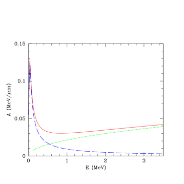
Figure 7: The coefficients ${\cal A}_{\rm\scriptscriptstyle I}(E)$ (dashed blue), ${\cal A}_{e}(E)$ (dotted green) and ${\cal A}(E)$ (solid red) as functions of the kinetic energy $E$ of an $\alpha$ particle projectile. The background plasma is equimolar DT with electron density $n_{e}=1.0\times 10^{25}\,{\rm cm}^{-3}$ and electron-ion temperatures $T_{e}=10\,{\rm keV}$ and $T_{\rm\scriptscriptstyle I}=10\,{\rm keV}$.

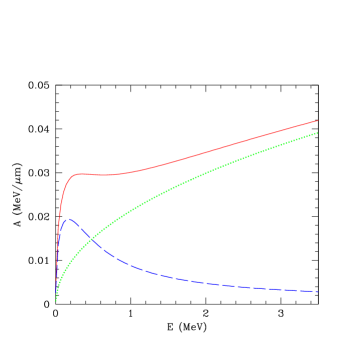
Figure 8: As in Fig. 7, except $T_{e}=10\,{\rm keV}$ and $T_{\rm\scriptscriptstyle I}=100\,{\rm keV}$. The crossover energy $E=E_{\rm\scriptscriptstyle C}$ where ${\cal A}_{e}(E)={\cal A}_{\rm\scriptscriptstyle I}(E)$ is about the same in both Figures; however, the peak value of the coefficient ${\cal A}_{\rm\scriptscriptstyle I}$ is inversely proportional to $T_{\rm\scriptscriptstyle I}$.

Figures 9 and 10 illustrate the number density scaling of the ${\cal A}$-coefficients by plotting ${\cal A}_{e}(E)/n_{e}$ and ${\cal A}_{\rm\scriptscriptstyle I}(E)/n_{e}$, as a function of the $\alpha$ particle energy $E$, over a wide range of electron densities: $n_{e}=10^{25}$, $10^{26}$, and $10^{27}\,\,{\rm cm}^{-3}$. As before, the electron temperature is $T_{e}=10\,{\rm keV}$ and the ion temperatures are $T_{\rm\scriptscriptstyle I}=10\,{\rm keV}$ and $T_{\rm\scriptscriptstyle I}=100\,{\rm keV}$, respectively.

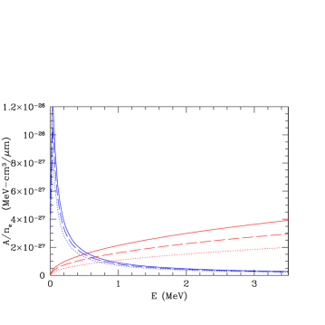
Figure 9: The $A$-coefficients for electrons and ions as a function of the $\alpha$ particle projectile energy $E$ in an equimolar DT plasma with equal electron and ion temperatures, $T_{e}=T_{\rm\scriptscriptstyle I}=10$ keV. The solid lines correspond to $n_{e}=1.0\times 10^{25}\,{\rm cm}^{-3}$, the dashed lines to $n_{e}=1.0\times 10^{26}\,{\rm cm}^{-3}$, and the dotted lines to $n_{e}=1.0\times 10^{27}\,{\rm cm}^{-3}$. In each case, the $A$-coefficient has been rescaled by the corresponding number density $n_{e}$. The slowly rising (red) curves are those for ${\cal A}_{e}$, while the sharply peaked (blue) curves are for ${\cal A}_{\rm\scriptscriptstyle I}$.

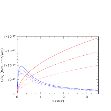
Figure 10: As in Fig. 9, except with $T_{e}=10\,{\rm keV}$ and $T_{\rm\scriptscriptstyle I}=100\,{\rm keV}$.

Because the ${\cal A}$-coefficients are proportional to the Debye wave number squared, a quantity proportional to $n_{e}$, it is no surprise that ${\cal A}_{\rm\scriptscriptstyle I}$ and ${\cal A}_{e}$ approximately scale with $n_{e}$. The Debye wave number also appears inside the logarithm and the dielectric function, and for electrons this produces a much more pronounced effect than for the much heavier ions: while ${\cal A}_{\rm\scriptscriptstyle I}/n_{e}$ is almost independent of $n_{e}$, the electron component ${\cal A}_{e}/n_{e}$ varies by a factor of two over the range of $n_{e}$.

Appendix B Asymptotic Limits

We shall extract the large and small energy limits of the ${\cal A}_{b}(v_{p})$ function for the various plasma species $b$ from the general expressions in BPS bps . The energy is given by $E=m_{p}v_{p}^{2}/2$, where $m_{p}$ and $v_{p}$ are the mass and speed of the particle moving through the plasma, the projectile $p$. We shall obtain the large and small limits of the projectile energy $E$ as compared to a typical plasma temperature $T$.

B.1 ${\bf E\ll T}$: Electrons and Ions

In the low velocity limit, ${\cal A}_{b}(v_{p})$ vanishes linearly with $v_{p}$, and so we write

$$v_{p}\to 0\,:$$ (151)

$${\cal A}_{b}(v_{p})=\frac{e_{p}^{2}\,\kappa_{b}^{2}}{4\pi}\,\left(\frac{\beta_{b}m_{b}}{2\pi}\right)^{1/2}v_{p}\,\left\{A_{b}^{\rm\scriptscriptstyle C}+A_{b}^{\Delta Q}\right\}\,,$$

with two constants $A_{b}^{\rm\scriptscriptstyle C}$ and $A_{b}^{\Delta Q}$. These two constants arise from the low velocity limit of the classical and quantum pieces of Eq. (140). The classical piece has already been calculated by BPS, where it is contained in their Eq. (9.9), so there is no need to do it here. The result is:

$$A_{b}^{\rm\scriptscriptstyle C}=\frac{2}{3}\left[\ln\left(\frac{16\pi}{e_{p}e_{b}\,\beta_{b}\kappa_{\rm\scriptscriptstyle D}}\,\frac{m_{pb}}{m_{b}}\right)-\frac{1}{2}-2\gamma\right]\,,$$ (152)

in which $m_{pb}$ is the reduced mass defined in Eq. (143) in the previous Appendix, and $\gamma=0.577\dots$ is Euler’s constant, and

$$\kappa_{\rm\scriptscriptstyle D}^{2}={\sum}_{b}\,\kappa_{b}^{2}={\sum}_{b}\,\beta_{b}\,e_{b}^{2}\,n_{b}\,.$$ (153)

To bring out the size of this classical part, we define a plasma coupling by

$$g_{pb}=\frac{e_{p}e_{b}\beta_{b}\kappa_{\rm\scriptscriptstyle D}}{4\pi}=\frac{e_{p}e_{b}}{4\pi\lambda_{\rm\scriptscriptstyle D}}\,\frac{1}{T_{b}}\,,$$ (154)

in which $\lambda_{\rm\scriptscriptstyle D}=1/\kappa_{\rm\scriptscriptstyle D}$ is the Debye length and $T_{b}=1/\beta_{b}$ is the temperature of plasma species $b$. Then we may write

$$A_{b}^{\rm\scriptscriptstyle C}=\frac{2}{3}\left[\ln\left(\frac{4}{g_{pb}}\,\frac{m_{pb}}{m_{b}}\right)-\frac{1}{2}-2\gamma\right]\,,$$ (155)

which shows that $A_{b}^{\rm\scriptscriptstyle C}>0$, since $g_{pb}$ must be small for our perturbative computation to hold. Note that when the electron and ion temperatures are not vastly different, the ions dominate in the low velocity limit (151) by a factor $(m_{i}/m_{e})^{1/2}$. Moreover, since $\kappa^{2}\sim 1/T$, this ionic contribution to the ${\cal A}$-coefficient has the temperature factor $T_{\rm\scriptscriptstyle I}^{-3/2}$ and thus increases as the ion temperature is lowered. The corrections to the low energy limit (151) are of relative order $E/T$.

The low velocity limit of the quantum correction Eq. (149) above was not previously calculated in BPS because there the low velocity limit of $dE/dx$ was used only to compare with a computer simulation involving classical dynamics, and therefore the quantum correction was not needed. The needed quantum part is contained in Eq. (10.27) of BPS which provides the limit

$$v_{p}\to 0\,:$$

$$\qquad\qquad A_{b}^{\Delta Q}=-\frac{1}{3}\beta_{b}m_{b}\int_{0}^{\infty}dv_{pb}\,v_{pb}\,\exp\left\{-\frac{1}{2}\,\beta_{b}m_{b}v_{pb}^{2}\right\}\left[2\,{\rm Re}\,\psi\left(1+i\eta_{pb}\right)-\ln\eta^{2}_{pb}\right]\,.$$

(156)

To bring out the character of Eq. (156), we introduce a thermal velocity $\bar{v}_{b}$ by

$$\frac{1}{2}m_{b}\bar{v}_{b}^{2}=\frac{3}{2}\,T_{b}\,,$$ (157)

or

$$\bar{v}_{b}^{2}=\frac{3}{\beta_{b}m_{b}}\,,$$ (158)

and a corresponding quantum parameter

$$\bar{\eta}_{pb}=\frac{e_{p}e_{b}}{4\pi\hbar\bar{v}_{b}}\,.$$ (159)

We then change the integration variable,

$$v_{pb}=\frac{e_{p}e_{b}}{4\pi\hbar\,\eta_{pb}}=\frac{e_{p}e_{b}}{4\pi\hbar}\,u=\bar{\eta}_{pb}\,\bar{v}_{b}\,u\,,$$ (160)

to obtain

$$A_{b}^{\Delta Q}=A_{b}^{\Delta Q}(\bar{\eta}_{pb})=-\bar{\eta}_{pb}^{2}\,\int_{0}^{\infty}du\,u\,\exp\left\{-\frac{3}{2}\bar{\eta}_{pb}^{2}\,u^{2}\right\}\left[2\,{\rm Re}\,\psi\left(1+\frac{i}{u}\right)+\ln u^{2}\right]\,.$$ (161)

If we introduce the Bohr radius $a_{0}=4\pi\hbar^{2}/e^{2}m_{e}$ and use the average squared thermal velocity definition (157), we can write

$${\bar{\eta}_{pb}}^{2}=\frac{1}{3}\,\left(\frac{e_{p}e_{b}}{e^{2}}\right)^{2}\,\frac{m_{b}}{m_{e}}\,\frac{1}{T_{b}}\,\frac{e^{2}}{4\pi a_{0}}\simeq\frac{1}{3}\,\left(\frac{e_{p}e_{b}}{e^{2}}\right)^{2}\,\frac{m_{b}}{m_{e}}\,\frac{27{\rm eV}}{T_{b}}\,.$$ (162)

Thus for the charge and mass of a typical projectile particle such as an alpha particle and for a typical hot plasma, we see that for the electrons in the plasma ${\bar{\eta}_{pe}}^{2}\ll 1$, while for the ions in the plasma ${\bar{\eta}_{pi}}^{2}\gg 1$ unless the ion temperature is somewhat larger than 10 keV.

For ${\bar{\eta}_{pe}}^{2}\ll 1$, the exponential does not rapidly damp large $u$ values, and so the relevant piece of the integrand is that with $u\gg 1$ where

$$\psi\left(1+\frac{i}{u}\right)\simeq\psi(1)=-\gamma\,,$$ (163)

leading to

$$A_{e}^{\Delta Q}(\bar{\eta}_{pe}) \simeq -\bar{\eta}_{pe}^{2}\,\int_{0}^{\infty}du\,u\,\exp\left\{-\frac{3}{2}\bar{\eta}_{pe}^{2}\,u^{2}\right\}\left[-2\,\gamma+\ln u^{2}\right]$$ (164)

$$= \frac{1}{3}\,\ln\left(\frac{3}{2}\,\bar{\eta}^{2}_{pe}\right)+\gamma\,.$$

Adding this result to the classical limit (152) gives the complete plasma electron contribution for a low energy projectile:

$$E\ll T\, {\bar{\eta}_{pe}}^{2}\ll 1\,:$$

$${\cal A}_{e}(v_{p}) = \frac{e_{p}^{2}\,\kappa_{e}^{2}}{4\pi}\,\left(\frac{\beta_{e}m_{e}}{2\pi}\right)^{1/2}\,\frac{v_{p}}{3}\left[\ln\left(\frac{8T_{e}m_{pe}^{2}}{m_{e}\hbar^{2}\,\kappa_{\rm\scriptscriptstyle D}^{2}}\right)-\gamma-1\right]\,.$$ (165)

For ${\bar{\eta}_{pi}}^{2}\gg 1$, the exponential rapidly damps large $u$ values, and so the relevant piece of the integrand is that with $u\ll 1$ where

$$\left[2\,{\rm Re}\,\psi\left(1+\frac{i}{u}\right)+\ln u^{2}\right]\simeq\frac{1}{6}\,u^{2}\,,$$ (166)

and thus

$${\bar{\eta}_{pi}}^{2}\gg 1\,:$$ (167)

$$A_{i}^{\Delta Q}(\bar{\eta}_{pi})\simeq-\frac{\bar{\eta}_{pi}^{2}}{6}\,\int_{0}^{\infty}du\,u^{3}\,\exp\left\{-\frac{3}{2}\bar{\eta}_{pi}^{2}\,u^{2}\right\}=-\frac{1}{27}\,{\bar{\eta}}_{pi}^{\,-2}\,.$$

Since this is a very small correction to $A_{i}^{\rm\scriptscriptstyle C}>0$, it may be neglected, and we may use the pure classical limit (152) for the ion contribution:

$$E\ll T\,, {\bar{\eta}_{pi}}^{2}\gg 1\,:$$

$${\cal A}_{i}(v_{p}) = \frac{e_{p}^{2}\,\kappa_{i}^{2}}{4\pi}\,\left(\frac{\beta_{i}m_{i}}{2\pi}\right)^{1/2}\,\frac{2v_{p}}{3}\left[\ln\left(\frac{16\pi}{e_{p}e_{i}\,\beta_{i}\kappa_{\rm\scriptscriptstyle D}}\,\frac{m_{pi}}{m_{i}}\right)-\frac{1}{2}-2\gamma\right]\,.$$ (168)

The total contribution of the ions in the plasma in this case is obviously

$$E\ll T\,,\quad{\bar{\eta}_{pi}}^{2}\gg 1\,:\qquad\qquad{\cal A}_{\rm\scriptscriptstyle I}(v_{p})={\sum}_{i}{\cal A}_{i}(v_{p})\,.$$ (169)

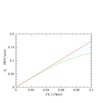
Figure 11: The ion contribution (green) plotted with the corresponding low-energy approximate form (red-linear) given by Eqs. (168) and (169). The plasma is equimolar DT with $T_{e}=T_{\rm\scriptscriptstyle I}=10\,{\rm keV}$ and $n_{e}=1.0\times 10^{25}\,{\rm cm}^{-3}$, and the projectile is an $\alpha$ particle. For these parameters, the plasma coupling is $g_{e}=0.0006$. Since the leading-order small-energy behavior is proportional to $v_{p}$, the graph of ${\cal A}_{\rm\scriptscriptstyle I}$ against $\sqrt{E}$ is linear in this region.

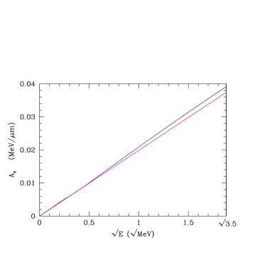
Figure 12: The electron contribution (blue) plotted with the corresponding low-energy approximate form (red-linear) given by Eq. (165). The plasma is the same as in the previous figure. Note that the linear approximation holds well into the $DT$ fusion production energy of $3.54\,{\rm MeV}$ for the $\alpha$ particles.

In Figs. 11 and 12 we plot the ion and electron ${\cal A}$-coefficients for an equimolar $DT$ plasma with an electron density $n_{e}=1.0\times 10^{25}\,{\rm cm}^{-3}$ and equal electron and ion temperatures $T_{e}=T_{\rm\scriptscriptstyle I}=10\,{\rm keV}$ against the square root of the projectile energy $\sqrt{E}$. We make this choice because in the small-energy regime the coefficients are linear in the projectile velocity; therefore, the graphs exhibit linear behavior until they start to depart from the low energy limit. Figures 13 and 14 plot the ${\cal A}$-coefficients for an equimolar DT plasma with $T_{e}=10\,{\rm keV}$ and $T_{\rm\scriptscriptstyle I}=100\,{\rm keV}$ and with an electron density $n_{e}=1.0\times 10^{25}\,{\rm cm}^{-3}$.

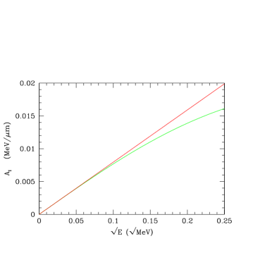
Figure 13: The ion contribution (green) plotted with the corresponding low-energy approximate form (red-linear) given by Eqs. (168) and (169). The plasma is equimolar DT with $T_{e}=10\,{\rm keV}$, $T_{\rm\scriptscriptstyle I}=100\,{\rm keV}$ and $n_{e}=1.0\times 10^{25}\,{\rm cm}^{-3}$, and the projectile is an $\alpha$ particle.

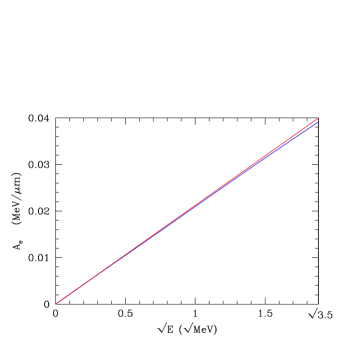
Figure 14: The electron contribution (blue) plotted with the corresponding low-energy approximate (red-linear) form (165). The plasma is the same as in the previous figure.

In Figs. 15 and 16 the temperatures are changed to $T_{e}=100\,{\rm keV}$ and $T_{\rm\scriptscriptstyle I}=10\,{\rm keV}$.

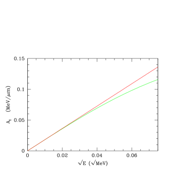
Figure 15: The ion contribution (green) plotted with the corresponding low-energy approximate (red-linear) form (168) and (169). The plasma is equimolar DT with $T_{e}=100\,{\rm keV}$, $T_{\rm\scriptscriptstyle I}=10\,{\rm keV}$ and $n_{e}=1.0\times 10^{25}\,{\rm cm}^{-3}$, and the projectile is an $\alpha$ particle.

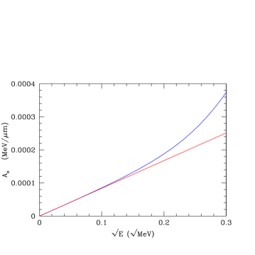
Figure 16: The electron contribution (blue) plotted with the corresponding low-energy approximate (red-linear) form (165). The plasma is equimolar DT with $T_{e}=100\,{\rm keV}$, $T_{\rm\scriptscriptstyle I}=10\,{\rm keV}$ and $n_{e}=1.0\times 10^{25}\,{\rm cm}^{-3}$, and the projectile is an $\alpha$ particle.

In Fig. 17 the coefficients ${\cal A}_{e}$ and ${\cal A}_{\rm\scriptscriptstyle I}$ are plotted together for three different temperatures.

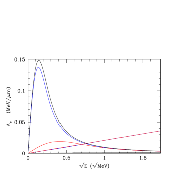
Figure 17: The coefficients $A_{e}$ and $A_{\rm\scriptscriptstyle I}$ are plotted together for three different temperatures for an equimolar DT plasma with an electron number density $n_{e}=1.0\times 10^{25}\,{\rm cm}^{-3}$. The ion contributions $A_{\rm\scriptscriptstyle I}$ peak to the left in the figure. The temperatures are: (i) $T_{e}=10\,{\rm keV}$ and $T_{\rm\scriptscriptstyle I}=10\,{\rm keV}$ (blue), (ii) $T_{e}=10\,{\rm keV}$ and $T_{\rm\scriptscriptstyle I}=100\,{\rm keV}$ (red), (iii) $T_{e}=100\,{\rm keV}$ and $T_{\rm\scriptscriptstyle I}=10\,{\rm keV}$ (black). The electron contributions $A_{e}$ for cases (i) and (ii) are almost equal, whereas for case (iii) ${\cal A}_{e}$ is very small.

B.2 $\bm{E\gg T}$: Total Ionic Contribution

For the total ionic contribution, it is convenient to first work out the regular part of the long-distance, dielectric contribution because it is the same for both cases of classical and quantum-mechanical scattering. With a trivial integration variable change, Eq. (144) presents this contribution as

$${\cal A}_{{\rm\scriptscriptstyle I},{\rm\scriptscriptstyle R}}^{\rm\scriptscriptstyle<}(v_{p})=\frac{e_{p}^{2}}{4\pi}\,\frac{1}{v_{p}^{2}}\,\frac{i}{2\pi}\int_{-v_{p}}^{+v_{p}}dv\,v\,\frac{\rho_{\rm\scriptscriptstyle I}(v)}{\rho_{\rm total}(v)}\,F(v)\,\ln\left(\frac{F(v)}{K^{2}}\right)\,,$$ (170)

where we now write

$$\rho_{\rm\scriptscriptstyle I}(v)={\sum}_{i}\,\rho_{i}(v)\,,$$ (171)

so that

$$\rho_{\rm total}(v)=\rho_{e}(v)+\rho_{\rm\scriptscriptstyle I}(v)\,,$$ (172)

with the weight functions $\rho$ given by Eq. (146). Assuming that the charges of the ions do not differ greatly from the charge of the electron, then $\kappa_{e}^{2}/\kappa^{2}_{\rm\scriptscriptstyle I}\simeq T_{\rm\scriptscriptstyle I}/T_{e}$ and the integrand of Eq. (170) involves a factor that has the behavior

$$\frac{\rho_{\rm\scriptscriptstyle I}(v)}{\rho_{\rm total}(v)}=\frac{1}{1+\rho_{e}(v)/\rho_{\rm\scriptscriptstyle I}(v)}\simeq\frac{1}{1+(m_{e}T_{\rm\scriptscriptstyle I}^{3}/m_{\rm\scriptscriptstyle I}T_{e}^{3})^{1/2}\,\exp\left\{m_{\rm\scriptscriptstyle I}v^{2}/2T_{\rm\scriptscriptstyle I}\right\}}\,,$$ (173)

where $m_{\rm\scriptscriptstyle I}$ is a typical ion mass. Thus, defining a typical ionic thermal velocity $v_{\rm\scriptscriptstyle T}$ by

$$m_{\rm\scriptscriptstyle I}\,v_{\rm\scriptscriptstyle T}^{2}=T_{\rm\scriptscriptstyle I}\,,$$ (174)

this factor remains unity up to the critical velocity $v_{\rm crit}$ defined by

$$v_{\rm crit}^{2}=v_{\rm\scriptscriptstyle T}^{2}\,\ln\left(\frac{m_{\rm\scriptscriptstyle I}\,T^{3}_{e}}{m_{e}\,T^{3}_{\rm\scriptscriptstyle I}}\right)\,,$$ (175)

after which it falls fairly rapidly to zero. The logarithmic factor in Eq. (175) is typically about a factor of 10. So $v_{\rm crit}$ is somewhat larger than an ion thermal velocity yet it is considerably smaller than the electron thermal velocity.

In this region in which the factor $\rho_{\rm\scriptscriptstyle I}(v)/\rho_{\rm total}(v)$ of the integrand is non-vanishing, the function [Eq. (148) above]

$$F(v)=-\int_{-\infty}^{+\infty}du\frac{\rho_{\rm total}(u)}{v-u+i\eta}$$ (176)

has the form

$$F(v)=\tilde{F}(v)=\kappa_{e}^{2}+F_{\rm\scriptscriptstyle I}(v)\,,$$ (177)

where

$$F_{\rm\scriptscriptstyle I}(v)=-\int_{-\infty}^{+\infty}du\frac{\rho_{\rm\scriptscriptstyle I}(u)}{v-u+i\eta}\,.$$ (178)

This is so because the velocity $v$, which must be less than $v_{\rm crit}$, is much less than the electron thermal velocity. Hence the electron part of $F(v)$ takes on its low velocity limit, the electron Debye wave number squared $\kappa_{e}^{2}$. We place the form (177) into Eq. (170) to obtain

$${\cal A}_{{\rm\scriptscriptstyle I},{\rm\scriptscriptstyle R}}^{\rm\scriptscriptstyle<}(v_{p})\simeq\frac{e_{p}^{2}}{4\pi}\,\frac{1}{v_{p}^{2}}\,\frac{i}{2\pi}\int_{-v_{p}}^{+v_{p}}dv\,v\,\frac{\rho_{\rm\scriptscriptstyle I}(v)}{\rho_{\rm total}(v)}\,\tilde{F}(v)\,\ln\left(\frac{\tilde{F}(v)}{\kappa_{e}^{2}}\right)\,.$$ (179)

Here we have replaced the arbitrary intermediate wave number $K$ by the electron Debye wave number $\kappa_{e}$ because now

$$v\to\infty\,:\qquad\qquad\frac{\tilde{F}(v)}{\kappa_{e}^{2}}\to 1-\frac{\omega_{\rm\scriptscriptstyle I}^{2}}{\kappa_{e}^{2}\,v^{2}}\,,$$ (180)

where

$$\omega_{\rm\scriptscriptstyle I}^{2}={\sum}_{i}\,\omega_{i}^{2}={\sum}_{i}\,\frac{e_{i}^{2}\,n_{i}}{m_{i}}\,,$$ (181)

and so $\ln(\tilde{F}(v)/\kappa_{e}^{2})$ vanishes for large $v$.

In order of magnitude,

$$\frac{\omega_{\rm\scriptscriptstyle I}^{2}}{\kappa_{e}^{2}\,v^{2}}\simeq\frac{T_{e}}{m_{\rm\scriptscriptstyle I}\,v^{2}}=\frac{T_{e}}{T_{\rm\scriptscriptstyle I}}\,\frac{v_{\rm\scriptscriptstyle T}^{2}}{v^{2}}\,.$$ (182)

Hence, since $v_{\rm\scriptscriptstyle T}^{2}$ is much less than $v_{\rm crit}^{2}$, unless $T_{e}$ is considerably larger than $T_{\rm\scriptscriptstyle I}$, the final factor in the integral (179), $\ln(\tilde{F}(v)/\kappa_{e}^{2})$, vanishes before $\rho_{\rm\scriptscriptstyle I}(v)/\rho_{\rm total}(v)$ departs significantly from unity. Hence we simply take $\rho_{\rm\scriptscriptstyle I}(v)/\rho_{\rm total}(v)=1$ and write

$${\cal A}_{{\rm\scriptscriptstyle I},{\rm\scriptscriptstyle R}}^{\rm\scriptscriptstyle<}(v_{p})\simeq\frac{e_{p}^{2}}{4\pi}\,\frac{1}{v_{p}^{2}}\,\frac{i}{2\pi}\int_{-v_{p}}^{+v_{p}}dv\,v\,\tilde{F}(v)\,\ln\left(\frac{\tilde{F}(v)}{\kappa_{e}^{2}}\right)\,.$$ (183)

The discussion above shows that when $v_{p}>v_{\rm crit}$, the limits of the integration may be replaced by $\pm\infty$. Recalling the definition (175) of the critical velocity $v_{\rm crit}$, and assuming that the projectile mass $m_{p}$ is about the same as the typical ion mass $m_{\rm\scriptscriptstyle I}$ in the plasma, we can now state that

$$E>T\,\ln\left(\frac{m_{\rm\scriptscriptstyle I}T_{e}^{3}}{m_{e}T_{\rm\scriptscriptstyle I}^{3}}\right)\,:$$

$${\cal A}_{{\rm\scriptscriptstyle I},{\rm\scriptscriptstyle R}}^{\rm\scriptscriptstyle<}(v_{p}) = \frac{e_{p}^{2}}{4\pi}\,\frac{1}{v_{p}^{2}}\,\frac{i}{2\pi}\int_{-\infty}^{+\infty}dv\,v\,\tilde{F}(v)\,\ln\left(\frac{\tilde{F}(v)}{\kappa_{e}^{2}}\right)\,.$$ (184)

We should note the convergence of the integral requires that the integration limits are to be taken in a rigorously symmetrical fashion with the integral performed between exactly $-v_{p}$ and $+v_{p}$ and then $v_{p}\to\infty$ taken. It is now a simple matter to evaluate this limiting form. Adding a semicircle in the upper half plane of radius $v_{p}$ gives a closed contour integral with no interior singularities that accordingly vanishes. Hence the value of the original integral is the negative of the integral over this large semicircle, an integral that is trivially performed using the limiting forms listed before. Thus

$$E>T\,\ln\left(\frac{m_{\rm\scriptscriptstyle I}T_{e}^{3}}{m_{e}T_{\rm\scriptscriptstyle I}^{3}}\right)\,:\qquad{\cal A}_{{\rm\scriptscriptstyle I},{\rm\scriptscriptstyle R}}^{\rm\scriptscriptstyle<}(v_{p})=-\frac{e_{p}^{2}}{4\pi}\,\frac{\omega_{\rm\scriptscriptstyle I}^{2}}{2\,v_{p}^{2}}\,.$$ (185)

With the long-distance, dielectric ionic contribution evaluated in the projectile high-energy limit, we can now compute the complete function ${\cal A}_{i}(v_{p})$ in this limit. To do so, we must distinguish two cases for the remaining hard scattering contribution.

B.2.1 $E\gg T$, $\eta_{pi}^{2}\gg 1$

As shown in detail in Sec. 10 of BPS, the classical scattering contribution dominates when the Coulomb parameter $\eta_{pi}$ is large, with the first quantum-mechanical correction of relative order

$$\eta_{pi}^{-2}=\left(\frac{4\pi\hbar v_{p}}{e_{p}e_{i}}\right)^{2}=\left(\frac{e^{2}}{e_{p}e_{i}}\right)^{2}\,\frac{2E}{\alpha^{2}\,m_{p}c^{2}}\,,$$ (186)

where $\alpha\simeq 1/137$ is the fine structure constant. In this classical limit, the scattering contribution is given by Eq. (142). For the previous evaluation of the dielectric contribution to hold, we must choose $K=\kappa_{e}$ so that this formula reads

$${\cal A}^{\rm\scriptscriptstyle C}_{i,{\rm\scriptscriptstyle S}}(v_{p}) = \frac{e_{p}^{2}\,\kappa_{i}^{2}}{4\pi}\,\left(\frac{\beta_{i}m_{i}}{2\pi}\right)^{1/2}\!\!v_{p}\int_{0}^{1}du\,u^{1/2}\,\exp\left\{-\frac{1}{2}\,\beta_{i}m_{i}v^{2}_{p}\,u\right\}$$ (187)

$$\qquad\left[-\ln\left(\beta_{i}\frac{e_{p}e_{i}}{4\pi}\,\kappa_{e}\,\frac{m_{i}}{m_{pi}}\,\frac{u}{1-u}\right)-2\gamma+2\right]\,.$$

Since $m_{i}v^{2}_{p}/2\sim E\gg T_{i}$, only small $u$ values are significant. Hence we can approximate $1-u=1$ within the logarithm and extend the integration limit to $u\to\infty$. With the variable change $(\beta_{i}m_{i}v_{p}^{2}/2)\,u=s^{2}$, we obtain the high-energy limit

$${\cal A}^{\rm\scriptscriptstyle C}_{i,{\rm\scriptscriptstyle S}}(v_{p}) = \frac{e_{p}^{2}}{4\pi}\,\frac{\omega_{i}^{2}}{v_{p}^{2}}\,\frac{4}{\sqrt{\pi}}\int_{0}^{\infty}ds\,s^{2}\,\exp\left\{-s^{2}\right\}\left[\ln\left(\frac{4\pi}{e_{p}e_{i}\kappa_{e}}\,\frac{m_{pi}v_{p}^{2}}{2}\right)-\ln s^{2}-2\gamma+2\right]\,,$$

where we have used $\kappa_{i}^{2}/\beta_{i}m_{i}=\omega_{i}^{2}$. Here we have the integrals

$$\frac{4}{\sqrt{\pi}}\int_{0}^{\infty}ds\,s^{2}\,\exp\left\{-s^{2}\right\}=1\,,$$ (189)

and

$$\frac{4}{\sqrt{\pi}}\int_{0}^{\infty}ds\,s^{2}\,\exp\left\{-s^{2}\right\}\,\ln s^{2} = \frac{2}{\sqrt{\pi}}\,\Gamma\left(\frac{3}{2}\right)\,\psi\left(\frac{3}{2}\right)=\psi\left(\frac{3}{2}\right)$$ (190)

$$= 2-\gamma-\ln 4\,.$$

Whence,

$${\cal A}^{\rm\scriptscriptstyle C}_{i,{\rm\scriptscriptstyle S}}(v_{p}) = \frac{e_{p}^{2}}{4\pi}\,\frac{\omega_{i}^{2}}{v_{p}^{2}}\,\left\{\ln\left(\frac{16\pi}{e_{p}e_{i}\kappa_{e}}\,\frac{m_{pi}v_{p}^{2}}{2}\right)-\gamma\right\}\,,$$ (191)

which, summed over all the ions in the plasma and combined with the previous long-distance result (185) yields the total contribution from the ions in the plasma:

$$E\gg T\,,\quad\eta_{pi}^{2} \gg 1\,:$$

$${\cal A}{\rm\scriptscriptstyle I}(v_{p}) = {\sum}_{i}\,{\cal A}_{i}(v_{p})={\sum}_{i}\,\left\{{\cal A}^{\rm\scriptscriptstyle C}_{i,{\rm\scriptscriptstyle S}}(v_{p})+{\cal A}^{\rm\scriptscriptstyle<}_{i,{\rm\scriptscriptstyle R}}(v_{p})\right\}$$ (192)

$$= \frac{e_{p}^{2}}{4\pi}\,\frac{1}{v_{p}^{2}}\,{\sum}_{i}\,\omega_{i}^{2}\,\,\left\{\ln\left(\frac{16\pi}{e_{p}e_{i}\kappa_{e}}\,\frac{m_{pi}v_{p}^{2}}{2}\right)-\gamma-\frac{1}{2}\right\}\,.$$

See Fig. 18 for a comparison of $A_{\rm\scriptscriptstyle I}$ with its asymptotic form at large energy.

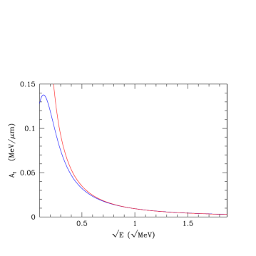
Figure 18: ${\cal A}_{\rm\scriptscriptstyle I}$ (blue curve) vs its large-energy (red curve) asymptotic form. The plasma is equimolar DT with $n_{e}=1.0\times 10^{25}\,{\rm cm}^{-3}$ and $T_{e}=T_{\rm\scriptscriptstyle I}=10\,{\rm keV}$.

B.2.2 $E\gg T$, $\eta_{pi}^{2}\ll 1$

In this case, we have the limit

$$v_{p}\to\infty\,:$$ (193)

$${\cal A}^{\rm\scriptscriptstyle C}_{i,{\rm\scriptscriptstyle S}}(v_{p})+{\cal A}^{\Delta Q}_{i}(v_{p})=\frac{e_{p}^{2}}{4\pi}\,\frac{1}{v_{p}^{2}}\,{\sum}_{i}\,\omega_{i}^{2}\ln\left(\frac{2m_{pi}v_{p}}{\hbar\kappa_{e}}\right)$$

which is contained in Eq. (10.42) of BPS. Adding this result to Eq. (185) now provides the complete $v_{p}\to\infty$ limit for the ion part of the ${\cal A}_{\rm\scriptscriptstyle I}$ coefficient:

$$E\gg T\,,\quad\eta_{pi}^{2}\ll 1\,:$$

$${\cal A}_{\rm\scriptscriptstyle I}(v_{p}) = \frac{e_{p}^{2}}{4\pi}\,\frac{1}{v_{p}^{2}}\,{\sum}_{i}\,\omega_{i}^{2}\left\{\ln\left(\frac{2m_{pi}v_{p}}{\hbar\kappa_{e}}\right)-\frac{1}{2}\right\}\,.$$ (194)

B.2.3 Rough Estimate For Either Case

The overall factor in the contribution of the ions to either of the high velocity limits (192) or (194) of the ${\cal A}$-coefficient has the same form as that of the electron contribution (209) given below, but with the major difference that the squared electron plasma frequency $\omega_{e}^{2}$ is replaced by a sum of squared ion plasma frequencies $\omega_{i}^{2}$, which are much smaller than the electron contribution by the ratio $m_{e}/m_{i}$. For a rough estimate of the size of the ionic contribution for high energy projectiles, we approximate the logarithm in either limit (192) or (194) by a constant $L$ of order one, and approximate $\omega_{\rm\scriptscriptstyle I}^{2}\simeq T_{\rm\scriptscriptstyle I}\,\kappa_{\rm\scriptscriptstyle I}/m_{\rm\scriptscriptstyle I}$ and $m_{\rm\scriptscriptstyle I}\simeq m_{p}$ to obtain

$$E\gg T\,:\qquad\qquad{\cal A}_{\rm\scriptscriptstyle I}(v_{p})\simeq\frac{e_{p}^{2}\,\kappa_{\rm\scriptscriptstyle I}^{2}}{4\pi}\,\frac{T_{\rm\scriptscriptstyle I}}{E}\,L\,.$$ (195)

B.3 $\bm{T\ll E\ll m_{p}T/m_{e}}$: Electronic Contribution

There is an intermediate range of projectile energies in which the projectile energy is much larger that the temperature, $E\gg T$, but yet not so large that we have $E\ll(m_{p}/m_{e})\,T\sim 10^{4}\,T$. We examine this range here.

We again need to work out its long-distance, dielectric contribution, and its short-distance scattering contribution.

B.3.1 Dielectric Part

In the energy range specified, the typical velocity in the dielectric function is small in comparison with the electron average thermal velocity and large in comparison with an ion average thermal velocity. Hence, in this range

$$F(v)\simeq\kappa_{e}^{2}-\frac{\omega_{\rm\scriptscriptstyle I}^{2}}{v^{2}}+\pi i\,\rho_{\rm total}(v)\,.$$ (196)

Here, in the dominant integration range,

$$\frac{\omega_{\rm\scriptscriptstyle I}^{2}}{\kappa_{e}^{2}\,v^{2}}\simeq\frac{T}{m_{\rm\scriptscriptstyle I}\,v^{2}}\ll 1\,,$$ (197)

and so we may simply write

$$F(v)\simeq\kappa_{e}^{2}+\pi i\,\rho_{\rm total}(v)\,.$$ (198)

Moreover, in the dominant integration range, the imaginary part $\pi\,\rho_{\rm total}(v)$ is small in comparison to $\kappa_{e}^{2}$. Writing Eq. (144) as

$${\cal A}^{\rm\scriptscriptstyle<}_{e,{\rm\scriptscriptstyle R}}(v_{p}) \simeq \frac{e_{p}^{2}}{4\pi}\,\frac{i}{2\pi}\int_{0}^{1}\!d\cos\theta\,\cos\theta\,\frac{\rho_{e}(v_{p}\cos\theta)}{\rho_{\rm total}(v_{p}\cos\theta)}\,\frac{1}{2}\,\Bigg{\{}$$ (199)

$$\qquad\qquad\Big{[}F(v_{p}\cos\theta)-F(-v_{p}\cos\theta)\Big{]}\ln\!\left(\frac{F(v_{p}\cos\theta)F(-v_{p}\cos\theta)}{K^{4}}\right)$$

$$\qquad\qquad\qquad+\Big{[}F(v_{p}\cos\theta)+F(-v_{p}\cos\theta)\Big{]}\ln\!\left(\frac{F(v_{p}\cos\theta)}{F(-v_{p}\cos\theta)}\right)\Bigg{\}}\,,$$

and using Eq. (198) with the imaginary part treated to first order,

$${\cal A}^{\rm\scriptscriptstyle<}_{e,{\rm\scriptscriptstyle R}}(v_{p}) \simeq -\frac{e_{p}^{2}}{4\pi}\,\int_{0}^{1}\!d\cos\theta\,\cos\theta\,\rho_{e}(v_{p}\cos\theta)\,\left\{\ln\!\left(\frac{\kappa_{e}^{2}}{K^{2}}\right)+1\right\}\,.$$ (200)

In our energy range Eq. (146) becomes

$$\rho_{e}(v)=\kappa_{e}^{2}\,\sqrt{\frac{\beta_{e}m_{e}}{2\pi}}\,v\,,$$ (201)

and so

$${\cal A}^{\rm\scriptscriptstyle<}_{e,{\rm\scriptscriptstyle R}}(v_{p}) \simeq -\frac{e_{p}^{2}}{4\pi}\,\kappa_{e}^{2}\,\sqrt{\frac{\beta_{e}m_{e}}{2\pi}}\,v_{p}\,\frac{1}{3}\,\left\{\ln\!\left(\frac{\kappa_{e}^{2}}{K^{2}}\right)+1\right\}\,.$$ (202)

B.3.2 Scattering Part

The electrons in the hot plasmas that we consider have such large velocities that their scattering off the projectiles is quantum mechanical. This is described by Eq. (10.41) of BPS which gives

$$\eta_{pe}\to 0\,:$$

$$\qquad{\cal A}^{\rm\scriptscriptstyle C}_{e,{\rm\scriptscriptstyle S}}(v_{p})+{\cal A}^{\Delta Q}_{e}(v_{p})=\frac{e_{p}^{2}\,\kappa^{2}_{e}}{4\pi}\,\left(\frac{\beta_{e}m_{e}}{2\pi}\right)^{1/2}\!\!v_{p}\int_{0}^{1}du\,u^{1/2}\,\exp\left\{-\frac{1}{2}\,\beta_{e}m_{e}v^{2}_{p}\,u\right\}$$

$$\qquad\qquad\qquad\qquad\qquad\qquad\qquad\frac{1}{2}\,\left[-\ln\left(\frac{\beta_{e}\hbar^{2}K^{2}}{2m_{pe}}\,\frac{m_{e}}{m_{pe}}\,\frac{u}{1-u}\right)-\gamma+2\right]\,.$$ (203)

With $E=\frac{1}{2}\,m_{p}v_{p}^{2}\ll m_{p}T/m_{e}$, the damping constant in the exponent $\beta_{e}m_{e}v_{p}^{2}/2$ is now small, not large as it was before. Hence the exponential may simply be replaced by unity, and we encounter the integrals

$$\int_{0}^{1}du\,u^{1/2}=\frac{2}{3}\,,$$ (204)

and

$$\int_{0}^{1}du\,u^{1/2}\ln\left(\frac{u}{1-u}\right)=\frac{2}{3}\,\left[2-\ln 4\right]\,.$$ (205)

Hence

$${\cal A}^{\rm\scriptscriptstyle C}_{e,{\rm\scriptscriptstyle S}}(v_{p})+{\cal A}^{\Delta Q}_{e}(v_{p}) = \frac{e_{p}^{2}\,\kappa^{2}_{e}}{4\pi}\,\left(\frac{\beta_{e}m_{e}}{2\pi}\right)^{1/2}v_{p}\,\frac{1}{3}\,\left[\ln\left(\frac{8T_{e}m_{pe}^{2}}{m_{e}\hbar^{2}K^{2}}\right)-\gamma\right]\,.$$ (206)

B.3.3 The Sum and a Rough Approximation

The sum of the dielectric part (202) and the scattering part (206) gives

$$E\gg T\,,\quad m_{e}E/m_{p} \ll T\,:~{}\text{or}~{}T\ll E\ll\frac{m_{p}}{m_{e}}\,T\,:$$

$${\cal A}_{e}(v_{p}) \simeq \frac{e_{p}^{2}\,\kappa^{2}_{e}}{4\pi}\,\left(\frac{\beta_{e}m_{e}}{2\pi}\right)^{1/2}\,\frac{v_{p}}{3}\,\left[\ln\left(\frac{8T_{e}m_{pe}^{2}}{m_{e}\hbar^{2}\kappa_{e}^{2}}\right)-\gamma-1\right]\,.$$ (207)

Figure 19 compares this high-energy approximation with the exact result. Figure 20 shows that the high and low energy approximations are quite similar.

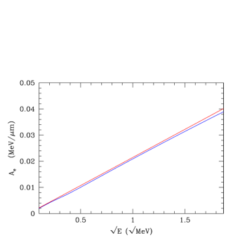
Figure 19: The coefficient $A_{e}$ (blue curve) compared with the (red curve) high-energy approximation (207). The plasma is equimolar DT with $n_{e}=1.0\times 10^{25}\,{\rm cm}^{-3}$ and $T_{e}=T_{\rm\scriptscriptstyle I}=10\,{\rm keV}$.

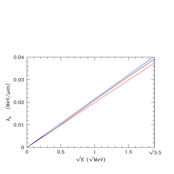
Figure 20: An $\alpha$ particle projectile moving in a equimolar $DT$ plasma with $T_{e}=T_{\rm\scriptscriptstyle I}=10$ keV and $n_{e}=1.0\times 10^{25}\,{\rm cm}^{-3}$. The (blue curve) low energy approximation (165) lies above the (black curve) exact result while the (red curve) high energy approximation (207) lies below the (black curve) exact result. Because $\kappa_{\rm\scriptscriptstyle D}^{2}=2\kappa_{e}^{2}$ for our equimolar $DT$ plasma, the two approximate forms (165) and (207) differ only by a factor of two inside the logarithm, and this leads to only slightly different slopes.

Again, to the rough, logarithmic accuracy that produced Eq. (195) for the ions, we now have for the electrons

$$E\gg T\,:\qquad\qquad{\cal A}_{e}(v_{p})\simeq\frac{e_{p}^{2}\,\kappa_{e}^{2}}{4\pi}\,\left(\frac{m_{e}}{m_{p}}\,\frac{E}{T_{e}}\right)^{1/2}\,L\,.$$ (208)

Note that this electron contribution has the leading temperature dependence given by the factor $\kappa_{e}^{2}\beta_{e}^{1/2}\sim T_{e}^{-3/2}$ and thus increases as the temperature is lowered. This is in marked contrast with the corresponding ion contribution given by Eq. (192) or Eq. (194) which, to within logarithmic accuracy, is independent of the temperature. The ions dominate at low projectile speeds as shown in Eq. (151), and their contribution at the low speeds also behaves as $T_{\rm\scriptscriptstyle I}^{-3/2}$ and so also increases as the temperature is lowered. On the other hand, as noted immediately below, the electrons greatly dominate at very high projectile speeds with a result that is completely independent of plasma temperatures. These remarks provide a qualitative description of the stopping power behavior in a plasma.

B.4 $\bm{E\gg m_{p}T/m_{e}}$: Electronic Contribution

The high velocity limit in this case has already been calculated by BPS in Eq. (10.43), which we simply quote here:

$$v_{p}\to\infty\,:$$ (209)

$${\cal A}_{e}(v_{p})=\frac{e_{p}^{2}}{4\pi}\,\frac{\omega_{e}^{2}}{v_{p}^{2}}\,\ln\left(\frac{2m_{pe}v_{p}^{2}}{\hbar\omega_{e}}\right)\,.$$

This limit is mostly academic, since the system enters the relativistic regime at these high velocities.

B.5 Energy Cross Over

As we have made explicit, the energy loss to the ions in the plasma dominates at low projectile energies while the loss is to the electrons at high projectile energies. Here we shall estimate the crossover point, the projectile energy at which the two types of loss mechanisms are comparable. We shall find that this occurs at a projectile energy that is much greater than a typical plasma temperature $T$, and so we will assume the limit $E\gg T$ in estimating the crossover point.

For the ions, the $E\gg T$ result (192) reads

$${\cal A}{\rm\scriptscriptstyle I}(v_{p}) = \frac{e_{p}^{2}}{4\pi}\,{\sum}_{i}\,\frac{\omega_{i}^{2}}{v_{p}^{2}}\,\left\{\ln\left(\frac{16\pi}{e_{p}e_{i}\kappa_{e}}\,\frac{m_{pi}v_{p}^{2}}{2}\right)-\gamma-\frac{1}{2}\right\}\,.$$ (210)

This holds provided that

$$\eta_{pi}^{-2}=\left(\frac{4\pi\hbar v_{p}}{e_{p}e_{i}}\right)^{2}=\left(\frac{e^{2}}{e_{p}e_{i}}\right)^{2}\,\frac{2E}{\alpha^{2}\,m_{p}c^{2}}\ll 1\,.$$ (211)

To put the total ion contribution in a convenient form, we again define a “total ion squared plasma frequency” by

$${\sum}_{i}\,\omega_{i}^{2}=\omega_{\rm\scriptscriptstyle I}^{2}\,,$$ (212)

replace the ion charge $e_{i}$ inside the logarithm by a typical value $e_{\rm\scriptscriptstyle I}$, and write $m_{pi}\simeq m_{p}/2$ to approximate the total ion contribution by

$${\cal A}_{\rm\scriptscriptstyle I}(v_{p}) \simeq \frac{e_{p}^{2}}{4\pi}\,\omega_{\rm\scriptscriptstyle I}^{2}\,\frac{1}{v_{p}^{2}}\left[\ln\left(\frac{16\pi}{e_{p}e_{\rm\scriptscriptstyle I}\kappa_{e}}\,\frac{E}{2}\right)-\gamma-\frac{1}{2}\right]\,.$$ (213)

Note that the only temperature dependence in this result is within the electron Debye wave number inside the logarithm. Hence the result only weakly depends upon the plasma temperatures.

A reasonably good approximation for the crossover projectile speed $v_{p}=v_{\rm\scriptscriptstyle C}$ should be obtained by equating the ion result (213) to the electronic result (207) which we repeat here using $\kappa_{e}^{2}=\beta_{e}m_{e}\,\omega_{e}^{2}$:

$${\cal A}_{e}(v_{p}) = \frac{e_{p}^{2}}{4\pi}\,\frac{\omega_{e}^{2}}{3}\,\left(\frac{2}{\pi}\right)^{1/2}\,\left(\frac{m_{e}}{T_{\rm\scriptscriptstyle C}}\right)^{3/2}\,v_{p}\,\left[\ln\left(\frac{\sqrt{8T_{e}m_{e}}}{\hbar\kappa_{e}}\right)-\frac{1}{2}\Big{(}\gamma-1\Big{)}\right]\,.$$ (214)

In equating the ion and electron approximations (213) and (214) we use the crossover energy defined by

$$E_{\rm\scriptscriptstyle C}=\frac{1}{2}m_{p}v_{\rm\scriptscriptstyle C}^{2}$$ (215)

to obtain

$$E_{\rm\scriptscriptstyle C}^{3/2}\left[\ln\left(\frac{\sqrt{8T_{e}m_{e}}}{\hbar\,\kappa_{e}}\right)-\frac{1}{2}(\gamma+1)\right] = T_{e}^{3/2}\left(\frac{9\pi}{16}\right)^{3/2}\!\left(\frac{m_{p}}{m_{e}}\right)^{3/2}\frac{\omega_{\rm\scriptscriptstyle I}^{2}}{\omega_{e}^{2}}\left[\ln\left(\frac{8\pi\,E_{\rm\scriptscriptstyle C}}{e_{p}e_{\rm\scriptscriptstyle I}\kappa_{e}}\right)-\gamma-\frac{1}{2}\right]\,.$$

It is important to note that this crossover point only depends upon the electron temperature $T_{e}$. The ion temperature $T_{\rm\scriptscriptstyle I}$ is of no relevance here.

Note that the results that we have obtained provide an approximate form for the total ${\cal A}$ coefficient as a function of the energy $E=m_{p}v^{2}_{p}/2$, ${\cal A}(E)={\cal A}_{e}(E)+{\cal A}_{\rm\scriptscriptstyle I}(E)$, namely

$${\cal A}(E)=\lambda E^{1/2}\,\left[1+\left(\frac{E_{\rm\scriptscriptstyle C}}{E}\right)^{3/2}\right]\,,$$ (217)

where

$$\lambda=\frac{e_{p}^{2}}{4\pi}\,\frac{\omega_{e}^{2}}{3}\,\left(\frac{1}{\pi}\right)^{1/2}\,\left(\frac{m_{e}}{T_{\rm\scriptscriptstyle C}}\right)^{3/2}\,\frac{2}{m_{p}^{1/2}}\,\left[\ln\left(\frac{\sqrt{8T_{e}m_{e}}}{\hbar\kappa_{e}}\right)-\frac{1}{2}\Big{(}\gamma-1\Big{)}\right]\,.$$ (218)

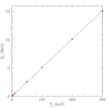
Figure 21: The solution of the crossover condition (LABEL:ECeqN) as a function of the electron temperature for an electron number density $n_{e}=1.0\times 10^{25}\,{\rm cm}^{-3}$. The straight line is a fit to these points, with $E_{\rm\scriptscriptstyle C}=51\,T_{e}$. Similar results obtain for the other densities, with the results presented in Eq. (220).

To return to assess the validity of our approximation for the cross over energy, we examine equimolar DT plasmas traversed by alpha particles of mass $m_{p}=m_{\alpha}$, charge $e_{p}=2e$, and initial energy $E_{0}=3.54$ MeV produced by DT fusion. In numerical terms for this case with the electron temperature $T_{e}$ and the crossover energy $E_{\rm\scriptscriptstyle C}$ measured in keV, and the electron number density $n_{e}$ measured in ${\rm cm}^{-3}$, the crossover relation (LABEL:ECeq) appears as

$$E_{\rm\scriptscriptstyle C}^{3/2}\,\left[\ln\left(5.796\times 10^{27}\,\frac{T_{e}^{2}}{n_{e}}\right)-1.577\right] = 188.1\,\,T_{e}^{3/2}\,\left[\ln\left(2.66\times 10^{28}\,\frac{T_{e}}{n_{e}}\,E_{\rm\scriptscriptstyle C}^{2}\right)-2.154\right]\,.$$

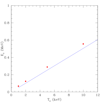
Figure 22: This figure displays the lower temperature region of the previous Fig. 21. Here the linear relation can deviate from the points which are solutions of the crossover relation (LABEL:ECeqN) with an error on the order of 10%.

As shown in Fig. 21 for one electron number density, we find that the crossover energies for different electron densities $n_{e}$ are nearly linear functions of $T_{e}$ given by

$$E_{\rm\scriptscriptstyle C}\simeq T_{e}\times\left\{\begin{array}[]{cc}48\,,\quad n_{e}=1.0\times 10^{24}\,{\rm cm}^{-3}\,,\\ 51\,,\quad n_{e}=1.0\times 10^{25}\,{\rm cm}^{-3}\,,\\ 53\,,\quad n_{e}=1.0\times 10^{26}\,{\rm cm}^{-3}\,.\end{array}\right.$$ (220)

Figure 22 shows that for energies below 10 keV or so, these linear relations break down by about 10 percent.

Appendix C The $G$ Function Simplified

Here we turn to the definition (LABEL:GGdef) of $G(T_{\rm\scriptscriptstyle I},T_{e};E_{0})$ in order to reduce it to a more manageable form. For convenience, we repeat this definition here:

$$G(T_{\rm\scriptscriptstyle I},T_{e};E_{0}) = \int_{0}^{\infty}dE\,F(E)\,e^{-S(E)}$$

$$\!\!\!\!\!\int_{0}^{E}\frac{dE^{\prime}}{E^{\prime}}\,\frac{e^{+S(E^{\prime})}}{\langle T{\cal A}(E^{\prime})\rangle}\,\left\{\theta\left(E_{0}-E^{\prime}\right)\,-\int_{E^{\prime}}^{\infty}dE^{\prime\prime}\sqrt{E^{\prime\prime}}\,\overline{\cal N}\,e^{-S(E^{\prime\prime})}\right\}\,,$$

where

$$\overline{{\cal N}}^{\,-1}=\int_{0}^{\infty}dE^{\prime}\,\sqrt{E^{\prime}}\,e^{-S(E^{\prime})}\,,$$ (222)

and

$$F(E)=E\,\frac{{\cal A}_{\rm\scriptscriptstyle I}(E){\cal A}_{e}(E)}{\langle T{\cal A}(E)\rangle}\,.$$ (223)

First we note that if $E^{\prime}<E_{0}$, the theta function in the curly braces is unity. Hence we can make use of the sum rule (90) to write

$$G(T_{\rm\scriptscriptstyle I},T_{e};E_{0})=G_{1}(T_{\rm\scriptscriptstyle I},T_{e};E_{0})+G_{2}(T_{\rm\scriptscriptstyle I},T_{e};E_{0})+G_{3}(T_{\rm\scriptscriptstyle I},T_{e};E_{0})\,,$$ (224)

where

$$G_{1}(T_{\rm\scriptscriptstyle I},T_{e};E_{0})=\int_{0}^{E_{0}}dE\,F(E)\,e^{-S(E)}\,\int_{0}^{E}\frac{dE^{\prime}}{E^{\prime}}\,\frac{e^{+S(E^{\prime})}}{\langle T{\cal A}(E^{\prime})\rangle}\,\int_{0}^{E^{\prime}}dE^{\prime\prime}\sqrt{E^{\prime\prime}}\,\,\overline{\cal N}\,e^{-S(E^{\prime\prime})}\,,$$

(225)

$$G_{2}(T_{\rm\scriptscriptstyle I},T_{e};E_{0})=\int_{E_{0}}^{\infty}dE\,F(E)\,e^{-S(E)}\,\int_{0}^{E_{0}}\frac{dE^{\prime}}{E^{\prime}}\,\frac{e^{+S(E^{\prime})}}{\langle T{\cal A}(E^{\prime})\rangle}\,\int_{0}^{E^{\prime}}dE^{\prime\prime}\sqrt{E^{\prime\prime}}\,\,\overline{\cal N}\,e^{-S(E^{\prime\prime})}\,,$$

(226)

and

$$G_{3}(T_{\rm\scriptscriptstyle I},T_{e};E_{0})=-\int_{E_{0}}^{\infty}dE\,F(E)\,e^{-S(E)}\int_{E_{0}}^{E}\frac{dE^{\prime}}{E^{\prime}}\,\frac{e^{+S(E^{\prime})}}{\langle T{\cal A}(E^{\prime})\rangle}\,\int_{E^{\prime}}^{\infty}dE^{\prime\prime}\sqrt{E^{\prime\prime}}\,\,\overline{\cal N}\,e^{-S(E^{\prime\prime})}\,.$$

(227)

First we show that $G_{3}$ may be neglected. For the very last pair of integrals in $G_{3}$, since the energies $E^{\prime}$ and $E^{\prime\prime}$ are larger than $E_{0}\gg T_{e}\,,\,T_{\rm\scriptscriptstyle I}$, the electron contribution to the ${\cal A}_{b}$ functions dominate, and so

$$S(E^{\prime\prime})-S(E^{\prime})=\frac{1}{T_{e}}\,\left(E^{\prime\prime}-E^{\prime}\right)\,.$$ (228)

This is a very large number unless $E^{\prime\prime}$ is near $E^{\prime}$. Hence, with corrections that will be of the very small order $T_{e}/E_{0}$, we have

$$\int_{E_{0}}^{E}\frac{dE^{\prime}}{E^{\prime}}\,\frac{e^{+S(E^{\prime})}}{\langle T{\cal A}(E^{\prime})\rangle}\,\int_{E^{\prime}}^{\infty}dE^{\prime\prime}\sqrt{E^{\prime\prime}}\,\,\overline{\cal N}\,e^{-S(E^{\prime\prime})}$$

$$\qquad\qquad\simeq\int_{E_{0}}^{E}\frac{dE^{\prime}}{E^{\prime}}\,\frac{1}{T_{e}{\cal A}_{e}(E^{\prime})}\,\sqrt{E^{\prime}}\,\,\overline{\cal N}\,\int_{E^{\prime}}^{\infty}dE^{\prime\prime}\exp\left\{-\frac{1}{T_{e}}\,\left(E^{\prime\prime}-E^{\prime}\right)\right\}$$

$$\qquad\qquad=\overline{\cal N}\,\int_{E_{0}}^{E}\frac{dE^{\prime}}{\sqrt{E}^{\prime}}\,\frac{1}{{\cal A}_{e}(E^{\prime})}\,,$$ (229)

and so, again since the electrons dominate the ${\cal A}_{b}$ functions in the high-energy regions that appear here,

$$G_{3}(T_{\rm\scriptscriptstyle I},T_{e};E_{0})\simeq-\int_{E_{0}}^{\infty}dE\,\frac{E}{T_{e}}\,{\cal A}_{\rm\scriptscriptstyle I}(E)\,e^{-S(E)}\,\overline{\cal N}\,\int_{E_{0}}^{E}\frac{dE^{\prime}}{\sqrt{E}^{\prime}}\,\frac{1}{{\cal A}_{e}(E^{\prime})}\,.$$ (230)

There is really no need to go any further in the evaluation of $G_{3}(T_{\rm\scriptscriptstyle I},T_{e};E_{0})$ since it has the exponentially small factor $\exp\{-S(E)\}$, with $E\geq E_{0}$. In this region, as we have noted, the electrons dominate and so $\exp\{-S(E)\}\simeq\exp\{-E/T_{e}\}$. Even for an electron temperature as high as 35 keV and for a $DT$ fusion alpha particle with $E_{0}=3.54$ MeV, this factor is $\exp\{-100\}\simeq 4\times 10^{-44}$.

For the evaluation of $G_{2}$, it is convenient to define

$$H(E^{\prime})=\int_{0}^{E^{\prime}}dE^{\prime\prime}\sqrt{E^{\prime\prime}}\,\overline{\cal N}\,e^{-S(E^{\prime\prime})}\,.$$ (231)

To isolate the leading pieces, we shall write

$$e^{\pm S(E)}=\pm\frac{\langle T{\cal A}(E)\rangle}{{\cal A}(E)}\,\frac{d}{dE}\,e^{\pm S(E)}$$ (232)

and integrate by parts. This will provide an extra explicit factor of a plasma temperature $T$ in the numerator, thereby yielding a small quantity.

The final double integral in the triple integral (226) defining $G_{2}$ now appears as

$$\int_{0}^{E_{0}}\frac{dE^{\prime}}{E^{\prime}}\,\frac{e^{+S(E^{\prime})}}{\langle T{\cal A}(E^{\prime})\rangle}\,\int_{0}^{E^{\prime}}dE^{\prime\prime}\sqrt{E^{\prime\prime}}\,\overline{\cal N}\,e^{-S(E^{\prime\prime})}$$

$$\qquad\qquad=\int_{0}^{E_{0}}dE^{\prime}\,\,\frac{H(E^{\prime})}{E^{\prime}\,{\cal A}(E^{\prime})}\frac{d}{dE^{\prime}}\,e^{+S(E^{\prime})}$$

$$\qquad\qquad\simeq\frac{H(E_{0})}{E_{0}\,{\cal A}(E_{0})}\,e^{+S(E_{0})}-\int_{0}^{E_{0}}dE^{\prime}\,e^{+S(E^{\prime})}\frac{d}{dE^{\prime}}\,\left[\frac{H(E^{\prime})}{E^{\prime}\,{\cal A}(E^{\prime})}\right]$$

$$\qquad\qquad\simeq\frac{H(E_{0})}{E_{0}\,{\cal A}(E_{0})}\,e^{+S(E_{0})}-\frac{\langle T{\cal A}(E_{0})\rangle}{{\cal A}(E_{0})}\,e^{+S(E_{0})}\left.\frac{d}{dE}\,\left[\frac{H(E)}{E\,{\cal A}(E)}\right]\right|_{E_{0}}+\cdots\,,$$

(233)

where the ellipsis represents the series resulting by further partial integrations. As we shall see, the second term in the last line of Eq. (233) is already negligible, and so are these omitted terms. The approximate equalities in Eq. (233) neglect lower limit terms since they result in exponentially small quantities from the remaining integration over $E$ in Eq. (226) because of the factor $\exp\{-S(E)\}$ with $E>E_{0}$. Here, to within very good accuracy,

$$H(E_{0})=1\,,$$ (234)

since the integral defining $H(E)$ has long since converged to its limiting value at $E=E_{0}$. Hence,

$$\int_{0}^{E_{0}}\frac{dE^{\prime}}{E^{\prime}}\,\frac{e^{+S(E^{\prime})}}{\langle T{\cal A}(E^{\prime})\rangle}\,\int_{0}^{E^{\prime}}dE^{\prime\prime}\sqrt{E^{\prime\prime}}\,\overline{\cal N}\,e^{-S(E^{\prime\prime})}$$

$$\qquad\qquad\simeq\frac{1}{E_{0}\,{\cal A}(E_{0})}\,e^{+S(E_{0})}\left\{1-\langle T{\cal A}(E)\rangle\left.E\,\frac{d}{dE}\,\left[\frac{1}{E\,{\cal A}(E)}\right]\right|_{E_{0}}\right\}\,.$$ (235)

Here, since at large energies the rate of energy variation is of order $1/E$,

$$\langle T{\cal A}(E)\rangle\left.E\,\frac{d}{dE}\,\left[\frac{1}{E\,{\cal A}(E)}\right]\right|_{E_{0}}\sim\,\frac{\langle T{\cal A}(E_{0})\rangle}{E_{0}\,{\cal A}(E_{0})}\,\sim\,\frac{T}{E_{0}}\,,$$ (236)

in which $T$ is a typical plasma temperature. The ratio $T/E_{0}$ is at most a few percent for the plasma configurations that we consider, and thus it is a good approximation to replace the curly braces in Eq.(235) by unity.

Recalling the definition (223) of $F(E)$ and then using the relation (232), we obtain

$$G_{2}(T_{\rm\scriptscriptstyle I},T_{e};E_{0}) \simeq \frac{1}{E_{0}\,{\cal A}(E_{0})}\,\int_{E_{0}}^{\infty}dE\,\left\{E\,\frac{{\cal A}_{\rm\scriptscriptstyle I}(E){\cal A}_{e}(E)}{\langle T{\cal A}(E)\rangle}\right\}\,\exp\left\{-\left[S(E)-S(E_{0})\right]\right\}$$

$$= -\frac{1}{E_{0}\,{\cal A}(E_{0})}\,\int_{E_{0}}^{\infty}dE\,E\,\frac{{\cal A}_{\rm\scriptscriptstyle I}(E){\cal A}_{e}(E)}{{\cal A}(E)}\,\frac{d}{dE}\,\exp\left\{-\left[S(E)-S(E_{0})\right]\right\}$$

$$= \frac{{\cal A}_{\rm\scriptscriptstyle I}(E_{0})\,{\cal A}_{e}(E_{0})}{{\cal A}^{2}(E_{0})}$$

$$+\frac{1}{E_{0}\,{\cal A}(E_{0})}\,\int_{E_{0}}^{\infty}dE\,\exp\left\{-\left[S(E)-S(E_{0})\right]\right\}\,\frac{d}{dE}\,\left\{E\,\frac{{\cal A}_{\rm\scriptscriptstyle I}(E){\cal A}_{e}(E)}{{\cal A}(E)}\right\}\,.$$

As before, we have the estimate

$$\frac{d}{dE}\,\left\{E\,\frac{{\cal A}_{\rm\scriptscriptstyle I}(E){\cal A}_{e}(E)}{{\cal A}(E)}\right\} \sim \frac{{\cal A}_{\rm\scriptscriptstyle I}(E){\cal A}_{e}(E)}{{\cal A}(E)}=\frac{\langle T{\cal A}(E)\rangle}{E\,{\cal A}(E)}\,\left\{E\,\frac{{\cal A}_{\rm\scriptscriptstyle I}(E){\cal A}_{e}(E)}{\langle T{\cal A}(E)\rangle}\right\}$$ (238)

$$\sim \frac{T}{E}\,\left\{E\,\frac{{\cal A}_{\rm\scriptscriptstyle I}(E){\cal A}_{e}(E)}{\langle T{\cal A}(E)\rangle}\right\}\,.$$

Here again $T$ represents a typical plasma temperature, and since the integration region starts at $E=E_{0}$, we have $T/E\leq T/E_{0}$, Since the factor in the curly braces in the last line in Eq. (238) is just the factor in the curly braces in the first line in Eq. (LABEL:geetwo), we see that the last line in Eq. (LABEL:geetwo) is of order $T/E_{0}$ times the first line, and thus gives a correction on the order of a few percent. We have found that, to within corrections of a few percent,

$$G_{2}(T_{\rm\scriptscriptstyle I},T_{e};E_{0}) \simeq \frac{{\cal A}_{\rm\scriptscriptstyle I}(E_{0})\,{\cal A}_{e}(E_{0})}{{\cal A}^{2}(E_{0})}\,.$$ (239)

The accuracy of the analytical approximation (239) for $G_{2}$ has been confirmed to this precision by direct numerical evaluation of its definition (226).

In summary, Eq. (224) expresses the $G$ function in three parts. The first part $G_{1}$ involves a triple integral that must be evaluated by numerical computation. This evaluation is simplified because, with the partition that we have made, the regions of integration that appear in $G_{1}$ are restricted to the finite interval $0<E<E_{0}$. For the second part $G_{2}$, the approximation (239) is sufficiently accurate for our purposes. The remainder $G_{3}$ is very small and we may simply set

$$G_{3}(T_{\rm\scriptscriptstyle I},T_{e};E_{0})=0\,.$$ (240)

References

- (1) R. L. Singleton Jr. and L. S. Brown, Plasma Phys. Control. Fusion 50, 124016 (2008).
- (2) L. S. Brown, D. L. Preston, and R. L. Singleton Jr., Phys. Rep. 410 (2005) 237-333, arXiv:physics/0501084.
- (3) G. S. Fraley, E.J. Linnebur, R. J. Mason, and R. L. Morse, Phys. Fluids 17 (1974) 474.
- (4) C-K. Li and R .D. Petrasso, Phys. Rev. Lett. 70, 3059 (1993).
- (5) K. A. Long and N. A. Tahir, Nucl. Fusion 26, 555 (1986).
- (6) G. Dimonte and J. Daligault, Phys. Rev. Lett. 101, 135001 (2008).
- (7) E. M. Lifshitz and L. P. Pitaevskii, Physical Kinetics, Volume 10 of the Course of Theoretical Physics, § 29, Pergamon Press, Oxford, 1981.
- (8) L. S. Brown and R. L. Singleton Jr., Phys. Rev. E 76, 066404 (2007).