Magnetostatic fields in tubular nanostructures

Abstract

The non-uniform magnetostatic field produced by the equilibrium and non equilibrium magnetic states of magnetic nanotubes has been investigated theoretically. We consider magnetic fields produced by actual equilibrium states and transverse and vortex domain walls confined within the nanostructure. Our calculations allow us to understand the importance of the magnetostatic field in nanomagnetism, which is frequently considered as a uniform field. Moreover, our results can be used as a basis for future research of others properties, such as the investigation of spin waves when domain walls are present, or the motion of a magnetic particle near a magnetic field.

I Introduction

Structures of nanometric dimensions are strongly dependent of size and shape mainly due to the fact that the characteristic scales of many physical phenomena are comparable to the dimensions of current nanostructures. Magnetism makes no exception and fundamental research of nanomagnets is further fuelled by their prospective applications into technological devices WAB+01 ; GBH+02 and biomedical applications ET03 ; Lee07 . The implementation of nanomagnets into potential devices requires a deep control of their physical properties; hence it is very important to control the shape and size of the nanoparticles which are crucial to determine their magnetic properties. Within currently available nanostructures, nanotubes made from 3d transition metals and their alloys are of particular importance, since the nanotube topologies provide us of two surfaces for modification, allowing the generation of multifunctional magnetic nanoparticles. Clearly, a technology capable to modify different surfaces would be highly desirable Eisenstein05 .

More recently hollow tubular nanostructures have been synthesized SRH+05 ; NCM+05 ; WLL+05 ; TGJ+06 and may be useful for applications in biotechnology, because low density magnetic nanotubes (MNs) can float in solutions and are more suitable for in vivo applications Eisenstein05 . In recent years, the magnetism of planar and circular nanowires has been intensely investigated, while MNs have received less attention, although MNs do not exhibit magnetic vortex cores or Bloch points Hertel04 , leading to a different behaviour with a more controllable reversal process.

It is well know that changes in the cross section of the MNs strongly affect the reversal mechanism and the overall magnetic behaviour WLL+05 ; DKG+07 ; ELA+07-1 ; ELA+07-2 ; LSC+09 . Recent articles have shown that MNs present three main equilibrium states: a uniform state (U), a mixed state (M) and a vortex state (V). With basis in theoretical models it has been argued that for nanotubes with outer radius less than $4L_{x}$ (where $L_{x}=\sqrt{2A/\mu_{0}M_{s}^{2}}$ is the exchange length, $M_{s}$ the saturation magnetization and $A$ the stiffness constant of the magnetic material) the magnetization is almost uniform and oriented principally along the cylindrical axis LSC+09 . We call this configuration uniform state. Also for nanotubes with $R\gtrsim 4L_{x}$ the magnetic equilibrium state correspond to the so-called mixed state, which is a mixture of U and V states WLL+05 ; LSC+09 ; LSS+07 ; CUB+07 . This state presents a uniform magnetization along the middle region of the tube and near the lower and upper surfaces the magnetization deviates from the uniformity in order to reduce the magnetostatic field LSC+09 . Finally, there is a transition from the M state to the vortex state as can be seen from figure 7 of LSC+09 .

On the other hand, it has been argued that domain wall propagation in nanostructures, which can be achieved by external fields or spin-currents, is of basic scientific and technological interest AAX+03 ; THJ+06 . More recently, it has been shown that the size-dependent reversal process in MNs occurs via DW nucleation and subsequent DW propagation. The DW microstructure depends on the tube cross section and can be a transverse wall (TW) for tube radius ($R$) smaller than a critical radius ($R_{c}(\beta)$), or a vortex wall (VW) for $R>R_{c}(\beta)$ LAE+07 ; EBJ+08 ; AEA+08 ; BEP+09 , where $\beta\equiv R_{i}/R$ is the ratio between the inner ($R_{i}$) and outer tube radius. The critical radius defined above depends on the magnetic material and on the shape factor $\beta$ and then it can be tailored manipulating its geometrical parameters. In polycrystalline systems, the critical radius, $R_{c}(\beta)$, ranges from a few nanometers to 20 nm approximately, and therefore, since experimentally fabricated MNs satisfy $R>R_{c}(\beta)$, we can expect that the propagation of a vortex DW be the dominant magnetization reversal mechanism for ferromagnetic nanotubes LAE+07 ; EBJ+08 ; AEA+08 ; BEP+09 .

Although the magnetostatic field of MNs with uniform magnetization has been already investigated EAA+08 ; PDE09 ; EAA+09 , an analytical model for the magnetostatic field produced by a MN with the above mentioned configurations, either equilibrium or transient states, has not yet been performed. Our intention is to fill this gap by using simple magnetization models LSC+09 ; LAE+07 . Since nanostructures are usually polycrystalline, the crystallographic orientations of the crystallites are random and, as a consequence, the average magnetic anisotropy of the particle is very small. In view of that, it will be neglected in our calculations KVL+03 ; CRE+00 . This paper is organized as follows: In Sec. II we present the magnetization models, including in Sec. II.1 the equilibrium states M and U and the VW, and then in Sec. II.2 we discuss the case of the TW. Results and discussions are summarized in Sec. III and conclusions in Sec. IV.

II Calculation of the magnetostatic fields

In this section we present explicit expressions to evaluate the magnetostatic field for nanotubes with the magnetization states described above. Within the continuum theory of ferromagnetism Aharoni96 , the magnetostatic field is given by $\mathbf{H}=-\nabla U$, where $U$ is the magnetostatic potential, which depends on the magnetization itself. The basic assumption we address in this paper is that the nanotubes we are considering are thin enough to avoid any dependence of the magnetization in the radial coordinate. In what follows we present the magnetization and the related magnetostatic field for the equilibrium states (U and M) and both DWs structures aforementioned.

II.1 Equilibrium states and vortex-like configurations

First, we consider nanotubes with vortex-like configurations, as the mixed state and the transient state with a VW confined within the tube. The magnetization of such magnetic configurations can be generally written as $\mathbf{M}(z)=M_{s}\mathbf{m}(z)=M_{s}(m_{\phi}(z)\hat{\phi}+m_{z}(z)\hat{\mathbf{z}})$, where $m_{z}(z)=\cos\Theta(z)$, and $m_{\phi}(z)=\sin\Theta(z)$, with $\Theta(z)$ being the angle between the local magnetization vector and the cylindrical $z$ axis. With this rather general form for the magnetization we can compute the magnetostatic field produced by $\mathbf{M}(z)$. Following the calculations of LSC+09 , the magnetostatic potential can be written as

$$U(\rho,z)=\frac{M_{s}}{2}\int\nolimits_{0}^{\infty}g(q)J_{0}(q\rho)\left[f_{s}+f_{v}\right]dq,$$ (1)

where $f_{s}$ and $f_{v}$ come from the surface and volumetric magnetic charges and can be written as

$$f_{s}\equiv-m_{z}(0)e^{-q|z|}+m_{z}(L)e^{-q|z-L|},$$ (2)

$$f_{v}\equiv-\int_{0}^{L}\frac{\partial m_{z}(y)}{\partial y}e^{-q|z-y|}dy.$$ (3)

In the potential we have also defined:

$$g(q)\equiv(R/q)\left[J_{1}(qR)-\beta J_{1}(\beta qR)\right],$$ (4)

where $J_{m}(x)$ are Bessel functions. The magnetostatic field associated with the above potential can be written as $\mathbf{H}=-\nabla U(\rho,z)$, and then, the cylindrical components of the field are $H_{\phi}=0$,

$$H_{\rho}=\frac{M_{s}}{2}\int\nolimits_{0}^{\infty}qg(q)J_{1}(q\rho)\left[f_{s}+f_{v}\right]dq,$$ (5)

$$H_{z}=-\frac{M_{s}}{2}\int\nolimits_{0}^{\infty}g(q)J_{0}(q\rho)\left[\frac{\partial f_{s}}{\partial z}+\frac{\partial f_{v}}{\partial z}\right]dq.$$ (6)

At this point we are in position to calculate the magnetostatic field through the reversal process for MNs, as well as to investigate the changes in the magnetostatic field when the equilibrium state is properly considered. In what follows we will use the equations above to calculate the magnetostatic field for the M state and the vortex DW.

II.1.1 Equilibrium magnetization states

The arrangement of magnetic moments in a MN with small radius can be seen as a uniform state in the middle region of the tube, but with vortex-like deviations of the magnetization located at the tube ends WLL+05 ; LSC+09 ; LSS+07 ; CUB+07 . This mixed state has been observed by micromagnetic simulations WLL+05 ; LSS+07 ; CUB+07 and studied theoretically LSC+09 . It has been shown that two equilibrium states can be studied with the model for the M state. In other words, the U state is a special case of the former, as we will see later. The model we use for the M state is given by the function LSC+09

$$\Theta(z)=\left\{\begin{array}[]{c}\theta_{0}\left(d-z\right)/d\text{ \ \ \ \ \ \ \ \ \ for }0\leq z\leq d\\ 0\text{ \ \ \ \ \ \ \ \ \ \ \ \ \ \ \ \ \ \ for }d\leq z\leq L-\lambda\\ \theta_{L}\left(z-L+\lambda\right)/\lambda\text{ \ \ \ \ for }L-\lambda\leq z\leq L\end{array}\right.$$ (7)

where $d$ and $\lambda$ are the dimensions of the regions where the magnetization deviates from the $z$-axis. In the model, $\theta_{0}$ and $\theta_{L}$ correspond to angles between the magnetization and the $z$-axis evaluated at the tube ends. Note that we obtain the uniform magnetization state in the limit $m_{z}(0)=m_{z}(L)=1$ ($\theta_{0}=\theta_{L}=0$) which occurs approximately for a radius smaller than 4$L_{x}$ LSC+09 . The parameters of the model are such that they minimize the total energy for each set of geometrical parameters. For simplicity we consider symmetric nanotubes, that is, tubes without difference between both tube ends. In those cases the four parameters ($d$, $\lambda$, $\theta_{0}$, $\theta_{L}$) variational problem is reduced to a two parameters variational problem, when $d=\lambda$ and $\theta_{0}=\theta_{L}$ LSC+09 . Then, $f_{s}$ and $f_{v}$ become

$$f_{s}^{M}=\cos\theta_{0}\left(-e^{-q|z|}+e^{-q|z-L|}\right),$$ (8)

$$f_{v}^{M}=\frac{\theta_{0}}{d}\int_{0}^{d}\sin(\theta_{0}\frac{d-y}{d})[e^{-q|z+y-L|}-e^{-q|z-y|}]dy.$$ (9)

With these quantities in hand we can compute the magnetostatic field $\mathbf{H}(\rho,z)$ at any point. Also, the uniform magnetization state is recovered with $\theta_{0}=0$, where the functions reduces to $f_{s}^{U}=-e^{-q|z|}+e^{-q|z-L|},$ $f_{v}^{U}=0$.

II.1.2 Vortex domain wall

The magnetization of the vortex wall in a nanotube can be expressed in a similar way to the magnetization of the mixed state, that is $\mathbf{M}(z)=M_{s}\sin\Theta(z)\hat{\phi}+M_{s}\cos\Theta(z)\hat{\mathbf{z}}$, but now

$$\Theta^{VW}(z)=\left\{\begin{array}[]{c}0\text{ \ \ \ \ \ \ \ \ \ \ \ \ \ \ \ \ \ \ \ \ \ \ \ \ \ \ for }0\leq z\leq z_{w}-\frac{\omega}{2}\\ \frac{\pi}{\omega}\left(z-z_{w}\right)+\frac{\pi}{2}\text{\ \ \ \ \ \ for }z_{w}-\frac{\omega}{2}\leq z\leq z_{w}+\frac{\omega}{2}\\ \pi\text{\ \ \ \ \ \ \ \ \ \ \ \ \ \ \ \ \ \ \ \ \ \ \ \ \ \ for }z_{w}+\frac{\omega}{2}\leq z\leq L\end{array}\right.$$ (10)

as presented in LAE+07 . Here $z_{w}$ is the location of the center of the vortex wall, and $w$ is the wall width. Within the above model, the magnetostatic field can be also expressed with equations (7) and (8), but now the functions $f_{s}$ and $f_{v}$ become

$$f_{s}^{VW}=-e^{-q|z|}-e^{-q|z-L|},$$ (11)

$$f_{v}^{VW}=\frac{\pi}{w}\int_{z_{w}-\frac{w}{2}}^{z_{w}+\frac{w}{2}}\cos\left(\pi\frac{y-z_{w}}{w}\right)e^{-q|z-y|}dy.$$ (12)

II.2 Transverse domain wall

The magnetization of the transverse wall in a nanotube can be expressed in a similar way to the vortex wall, but with $\mathbf{M}(z)=M_{s}\sin\Theta(z)\hat{\mathbf{x}}+M_{s}\cos\Theta(z)\hat{\mathbf{z}}$ LAE+07 , and $\Theta(z)$ being the same of the vortex wall. It can be noted that the main difference between vortex and transverse walls (in nanotubes) is the direction of the in-plane magnetization, which makes the nature of the wall properties to be different. The model that we use for the transverse wall LAE+07 leads us to understand some basic properties, like the DW width or the energy barrier for the reversal process. Here we are interested in the visualization of the magnetostatic field produced by a static domain wall. It can be shown that this field can be written as $\mathbf{H}=-\nabla U(\rho,\phi,z)$, without the usual axial symmetry of vortex-like states. The case of a vortex wall presents a magnetostatic potential independent of the angular coordinate $\phi$, which secures angular symmetry. Following LAE+07 , the field can be written as $\mathbf{H}^{TW}=H_{\rho}^{TW}\hat{\rho}+H_{\phi}^{TW}\hat{\phi}+H_{z}^{TW}\hat{\mathbf{z}}$. Provided the magnetostatic potential of the TW can be written as

$$U^{TW}=U^{VW}+A(\rho,z)\cos\phi,$$ (13)

the components of the dipole field created for the TW can then be expressed as

$$H_{\rho}^{TW}(\rho,\phi,z)=H_{\rho}^{VW}(\rho,z)+\frac{\partial A(\rho,z)}{\partial\rho}\cos\phi,$$ (14)

$$H_{\phi}^{TW}(\rho,\phi,z)=-A(\rho,z)\sin\phi,$$ (15)

$$H_{z}^{TW}(\rho,\phi,z)=H_{z}^{VW}(\rho,z)+\frac{\partial A(\rho,z)}{\partial z}\cos\phi,$$ (16)

where

$$A(\rho,z)=\frac{M_{s}}{2}\int\nolimits_{0}^{\infty}qg(q)J_{1}(q\rho)\varsigma(z,q)dq,$$ (17)

and

$$\varsigma(z,q)\equiv\int_{0}^{L}m_{x}(z^{\prime})e^{-q|z-z^{\prime}|}dz^{\prime}.$$ (18)

Here, $m_{x}(z)=\sin\Theta^{TW}(z)$, with $\Theta^{TW}(z)=\Theta^{VW}(z)$. The function $\varsigma(z,q)$ possesses the information about the DW microstructure and can be straightforwardly integrated. Finally, notice that the widths of the vortex and transverse walls are essentially different, and should be evaluated within the framework presented in LAE+07 .

III Results and discussion

In the above sections we have obtained explicit expressions to calculate the magnetostatic field for different magnetic states in nanotubes. In what follows we present plots of the magnetostatic field produced by the magnetic states relevant to nanotubes. We begin the discussion with the equilibrium states (U and M) and then we analyze the case of vortex and transverse walls propagating along the nanostructure.

III.1 Vector plots of the equilibrium states

As mentioned earlier, the uniform magnetization state ($\theta_{0}=0$) is a special case of the mixed state ($\theta_{0}>0$), and occurs when the tube radius is approximately less than 4$L_{x}$, provided the exchange energy dominates over the dipolar one LSC+09 . When $R>4L_{x}$ the magnetization at the tube ends is not entirely parallel to the cylindrical $z$ axis, instead it develops vortex domains at the ends in order to reduce the dipolar energy LSC+09 . The long range character of the dipolar interaction makes that the dipolar energy grows as $N^{2}$, whereas the exchange energy grows as $N$, with $N$ the number of atomic magnetic moments in the tube. Therefore, the edge vortex domains increases in size with the radius. In the language of the above equations, the size of the vortex domains is given by the parameters $\theta_{0}$ and $d$. As $R$ increases over 4$L_{x}$, $\theta_{0}$ and $d$ increases, as the reader can see from figures 5 and 6 in LSC+09 . To calculate the magnetostatic field we need to know the set of parameters ($\theta_{0},d$) which minimize the total energy of the mixed state. Using the expressions for the total energy of LSC+09 , we obtain for nanotubes with $\beta=0.9$ and $L=1000L_{x}$ different values of ($\theta_{0},d$) depending on their radius. These results are summarized in table LABEL:table1. Note that for $L=1000L_{x}$ the transition to a flux-closure vortex state occurs approximately at $R\approx 27L_{x}$ LSC+09 .

$$R/L_{x}$$

($\theta_{0},d$) for magnetic nanotubes with $\beta=0.9$ and $L=1000L_{x}$ as a function of their radius.

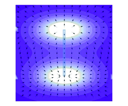
Figure 1: (Colour online). Magnetostatic field produced by a tube with uniform magnetization along the symmetry axis. The arrows have been normalized to the local strength of the field indicated by the colour. Parameters are indicated in the text.

The arrows in figure 1 show the normalized magnetostatic field for a uniformly magnetized MN with $R=4L_{x}$. The colour code indicates the strength of the field at each point; white colour indicates that the magnetostatic field is stronger at the tube ends because “magnetic charges” ($\sigma_{M}$) resides only at the surfaces such that $\sigma_{M}=\mathbf{M}\cdot\hat{\mathbf{n}}\neq 0$, with $\hat{\mathbf{n}}$ a unit vector normal to the surface of the sample Aharoni96 . Provided that the U and M states (as well as the vortex wall) can be represented with $\mathbf{M}=M_{\phi}(z)\hat{\phi}+M_{z}(z)\hat{\mathbf{z}}$, it follows that the surface magnetic charges are given by $\sigma_{M}(z)=M_{z}(z)\hat{\mathbf{z}}\cdot\hat{\mathbf{n}}$, where $z=0$ or $L$. In the upper surface of the tube ($z=L$) $\hat{\mathbf{n}}=\hat{\mathbf{z}}$ and then $\sigma_{M}(L)=M_{z}(L)$, whereas in the lower surface $\hat{\mathbf{n}}=-\hat{\mathbf{z}}$, and $\sigma_{M}(0)=-M_{z}(0)$. If the actual equilibrium state is the U or the M state, we find positive magnetic charges ($\sigma_{M}(L)>0$) located at the upper surface, and this region behaves like a source of charges, as in figure 1; in elementary electromagnetism the field lines emanate from positive charges. Conversely, in the lower surface $\sigma_{M}(0)<0$ and the region behaves like a sink of charge (the field lines converge to these points). It can be shown that for nanotubes in the mixed state, the dipole field looks very similar to the one plotted in figure 1. As a consequence, we do not present the same plots for tubes in the mixed state, instead we show in figure 2 the dependence of the magnitude of the dipole field ($H_{d}=\sqrt{H_{\rho}^{2}+H_{z}^{2}}$) with the radial coordinate for different tube radius and $z=1050L_{x}$ (just $50L_{x}$ above the upper surface of the tube). We have normalized all the curves to $M_{s}(R/L_{x})^{2}$, and in order to remark the difference between the U state and the M state, we present groups of curves for both states.

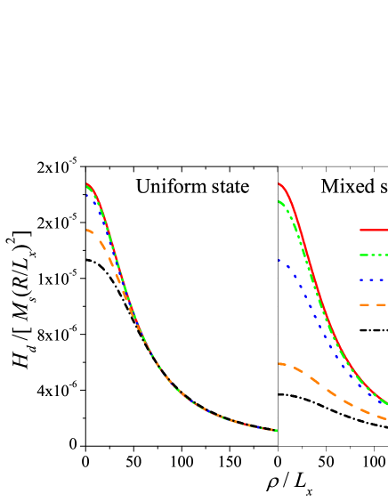
Figure 2: (Colour online). Magnetostatic field strength as a function of the radial coordinate and $z=1050L_{x}$. The left panel shows curves for the uniform state and the right panel shows the magnetostatic field for the mixed state. Different curves represent different tube radius, as depicted in the figure, and parameters have been taken from table 1.

We observe that a proper consideration of the equilibrium state reduces considerably the dipole field. This effect becomes critical as the tube radius is increased, which increment the size of the vortex domains of the mixed state LSC+09 . It is worth to mention about the importance of a proper consideration of the actual magnetic state in tubular nanostructures. In the sake of simplicity, it is a very common practice in magnetism to approximate the magnetization as a uniform field, in spite that uniform magnetization can be achieved (at zero applied field) only in nanostructures with dimensions of the order of the exchange length Kravchuk ; bookchapter , or when the nanoparticle is an ellipsoid with the appropriate size. Moreover, cylindrical magnetic nanowires and nanotubes are frequently consider as infinite structures, and only in this limit the approximation of a uniform dipole field becomes plausible, because the cylindrical nanostructures can be considered as ellipsoids only if they are infinitely long. However, actual magnetic nanostructures are not infinite and finite size effects can be relevant. It is well known that the dipole field produced by a nanoparticle with an ellipsoidal shape is uniform if its size is below the single domain limit (in absence of an external field) Aharoni96 . In this limit one can safely write the dipole field in terms of the corresponding demagnetizing factor: $\mathbf{H}_{d}=-N\mathbf{M}$.

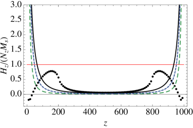
Figure 3: (Colour online). Component of the dipole field along the MN axis as a function of coordinate $z$. The fields have been normalized to $N_{z}M_{s}$, where $N_{z}$ is the corresponding demagnetizing factor. The long dashed line corresponds to the U state for $R/L_{x}=4$. The short dashed line corresponds to the U state and $R/L_{x}=10$. The thick solid line correspond to U state and $R/L_{x}=20$ whereas the circles correspond to the M state for $R/L_{x}=20$. The horizontal line illustrates the strength of the dipole field calculated in the usual ellipsoid-like approximation for uniform magnetization: $H_{d}=-N_{z}M_{s}$.

The difference between uniform and non-uniform dipolar fields is illustrated in figure 3, where we have plotted $H_{z}$, the component of the magnetostatic field along the tube axis, as a function of $z$ for different tube radius and magnetic states. The horizontal solid line depicts the strength of the (uniform) dipole field ($N_{z}M_{s}$) produced by an infinite MN with uniform magnetization, whereas the long dash, short dash and solid lines correspond to the field produced by a MN with a uniform magnetization state with radius $R/L_{x}=4$, 10 and 20, respectively. The circles correspond to the dipole field produced by a MN with a mixed state rather the incorrect uniform magnetization state, and with $R/L_{x}=20$. The fields have been normalized to $N_{z}M_{s}$, where $N_{z}=N_{z}(R,L,\beta)$ is the corresponding demagnetizing factor for a nanotube ELA+07-1 ; Beleggia06 .

III.2 Vector plots for a vortex wall

In order to illustrate the basic characteristics of the magnetostatic field produced by a MN with a vortex domain wall, we have chosen nanotubes with $\beta=0.9$, $L=1000L_{x}$ and $R=10L_{x}$. Following a previous work by some of us LAE+07 , we can calculate numerically the DW width ($w$) by minimizing the total energy including exchange. It is found that $w=w(\beta,R)$, and for the values mentioned above we obtain a wall width $w=109L_{x}$. In figure 4 we show the magnetostatic field normalized to his strength for a vortex wall located at $z_{w}=750L_{x}$, whereas figure 5 shows the same plot for the VW confined at the middle of the tube ($z_{w}=500L_{x}$).

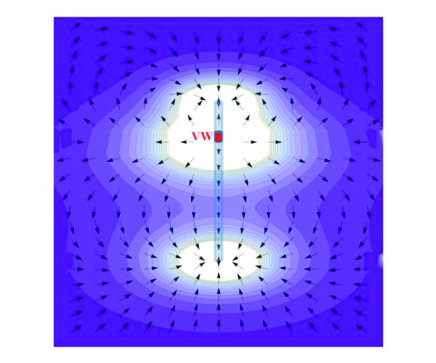
Figure 4: (Colour online). Vector plot of the magnetostatic field for a ferromagnetic nanotube with a vortex domain wall located at $z_{w}=750L_{x}$. The colours indicate the strength of the magnetostatic field. Parameters are presented in the main text.

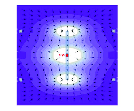
Figure 5: (Colour online). Vector plot of the magnetostatic field for a ferromagnetic nanotube with a vortex domain wall located at $z_{w}=500L_{x}$. The colours indicate the strength of the magnetostatic field. Parameters are presented in the text.

Both figures illustrate three regions where there are magnetic charge; upper and lower tube ends, and the region of the DW around the wall position $z_{w}$, which has been highlighted with red colour. There are negative surface charges at the tubes ends, because $\sigma_{M}(0)=-M_{z}(0)=-M_{s}<0$ and $\sigma_{M}(L)=M_{z}(L)=-M_{s}<0$. Also, there is a positive volume charge localized in the domain wall region. A volume magnetic charge Aharoni96 is given by $\rho_{M}=-\nabla\cdot\mathbf{M}$ , and thus in our case $\rho_{M}=-\partial M_{z}/\partial z$. Besides, $M_{z}=M_{s}\cos\Theta(z)$, and therefore, $\rho_{M}=M_{s}(\pi/w)\sin\Theta>0$, just in the DW region. Therefore, the DW acts as a source of magnetic charge. Note that we are considering here head-to-head DWs, and in order to analyze the case of tail-to-tail walls, we should replace $M_{z}$ by $-M_{z}$ and the corresponding magnetic charges must have the opposite sign as discussed here for head-to-head walls.

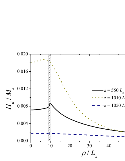
Figure 6: (Colour online). Strength of the magnetostatic field for a MN with a vortex domain wall located at $z_{w}/L_{x}=500$. Parameters are the same of figure 5 while the dashed region represent the region occupied by the magnetic matter.

Finally, in figure 6 we illustrate the strength of the dipolar field as a function of the distance to the z axis, and for different $z$ values. We have considered the same parameters as in figure 5 which means that we have magnetic matter just for $\rho/L_{x}=9-10$ and $z/L_{x}=0-1000$.

III.3 Vector plots for a transverse wall

To visualize the dipole field produced by a transverse wall, we have chosen MNs with the same parameters of the above section, that is $\beta=0.9$, $L=1000L_{x}$ and $R=10L_{x}$. Following a previous work LAE+07 we can calculate the transverse DW width ($w$) by minimizing the total energy, as stated before. Again, it is found that $w=w(\beta,R)$, and for the values mentioned above we obtain $w=7.67L_{x}$, a rather small value as compared to the corresponding DW width for the VW of the above section. The magnetic field for the transverse wall configuration is given by equations (14-16). Note that the angular component of the field $H_{\phi}$ is not zero (unless $\sin\phi=0$) and therefore the field does not present azimuthal symmetry as the magnetostatic field for the vortex DW. It can be shown that for the geometry discussed here, the vector field along the plane defined by $\phi=0$ lies completely in that plane, where $H_{\phi}(\phi=0)=0$. Along this plane it is found that the field is very similar to the field for the VW (see figure 5). This can be understood by noting that, mathematically, the field for the TW is very similar to the case of the VW. The main differences are the wall width and the term dependent on the angle $\phi$, and the function $A(\rho,z)$ defined in (17).

In figures 7 and 8 we show the magnetostatic field produced by the magnetization of a transverse DW located at $z_{w}=500L_{x}$. Figure 7 depicts the top view of the field along the plane $z=600L_{x}$, and figure 8 shows the plane $z=1200L_{x}$. Both plots represents the in-plane component of the field ($H_{\rho}^{TW}\hat{\rho}+H_{\phi}^{TW}\hat{\phi}$) normalized to their strengths given by the colour code. The central ring illustrates the top view of the nanotube. We have also included information about $H_{z}^{TW}$ which is given by the length of the arrows. It can be noted that near the ferromagnetic tube, the z component of the field is more important, and thus the arrows are smaller.

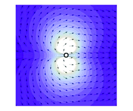
Figure 7: (Colour online). Magnetostatic field for a ferromagnetic nanotube with a transverse domain wall located at the middle of the tube ($z_{w}=500L_{x}$). The plot represent the top view of the field, at the plane $z=600L_{x}$. The colour indicates the strength of the magnetostatic field, and along the contours the value of the field is constant. Parameters are presented in the text.

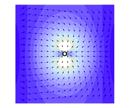
Figure 8: (Colour online). Magnetostatic field for a ferromagnetic nanotube with a transverse DW located at the middle of the tube. The plot represent the top view of the field at the plane $z=1200L_{x}$. The colours indicate the strength of the magnetostatic field. Along the contours the value of the field is constant. Parameters are presented in the text.

IV Final Remarks

In summary, we have investigated the dipole field produced by equilibrium and non-equilibrium domain wall states of magnetic nanotubes. Using a continuous model we have obtained simple expressions to evaluate the dipole fields. On one hand, we can conclude that the consideration of magnetic states, as the non-uniform mixed state instead the idealized uniform state, reduces considerably the magnetostatic field. Thus, it is important for researchers to have in mind this approach when they compare with experimental results, in order to avoid the overestimation of stray fields. On the other side, magnetic domain walls, which can be manipulated by external fields or spin-currents, introduce volumetric magnetic charges into the nanostructure. These charges move in the direction of the applied field if the DW is a head-to-head wall, and in the opposite direction if the wall is a tail-to-tail one. Finally, we have concluded that the magnetostatic field strongly depends on the mechanisms of magnetization reversal. Our results are intended to provide guidelines to use the magnetostatic field generated by tubular nanostructures in prospective applications such as the generation of a magnetic trap.

References

- (1) Wolf S A, Awschalom D D, Buhrman R A, Daughton J M, von Molnar S, Roukes M L, Chtchelkanova A Y and Treger M 2001 Science 294 1488.
- (2) Gerrits Th, van den Berg H A M, Hohlfeld J, Bar L and Rasing Th 2002 Nature (London) 418 509.
- (3) Emerich D F and Thanos C G 2003 Expert Opin. Biol. Ther. 3 655.
- (4) Lee D, Cohen R E and Rubner M F 2007 Langmuir 23 123
- (5) Eisenstein M 2005 Nat. Methods 2 484.
- (6) Son S J, Reichel J, He B, Schushman M and Lee S B 2005 J. Am. Chem. Soc. 127 7316.
- (7) Nielsch K, Castano F J, Matthias S, Lee W and Ross C A 2005 Adv. Eng. Mater. 7 217.
- (8) Wang Z K, Lim H S, Liu H Y, Ng S C, Kuok M H, Tay L L, Lockwood D J, Cottam M G, Hobbs K L, Larson P R, Keay J C, Lian G D and Johnson M B 2005 Phys. Rev. Lett. 94 137208.
- (9) Tao F, Guan M, Jiang Y, Zhu J, Xu Z and Xue Z 2006 Adv. Mater. (Weinheim, Ger.) 18 2161.
- (10) Hertel Riccardo, Kirschner Jürgen 2004 J. Magn. Magn. Mater. 278 L291.
- (11) Daub M, Knez M, Gosele U and Nielsch K 2007 J. Appl. Phys. 101 09J111.
- (12) Escrig J, Landeros P, Altbir D, Vogel E E and Vargas P 2007 J. Magn. Magn. Mater. 308 233.
- (13) Escrig J, Landeros P, Altbir D and Vogel E E 2007 J. Magn. Magn. Mater. 310 2448.
- (14) Landeros P, Suarez O J, Cuchillo A and Vargas P 2009 Phys. Rev. B 79 024404.
- (15) Lee Johyun, Suess Dieter, Schrefl Thomas, Hwan Oh Kyu and Fidler Josef 2007 J. Magn. Magn. Mater. 310 2445.
- (16) Chen A P, Usov N A, Blanco J M and Gonzalez J 2007 J. Magn. Magn. Mater. 316 e317.
- (17) Atkinson D, Allwood A, Xiong G, Cooke M D, Faulkner C C and Cowburn R P 2003 Nat. Mater. 2 85.
- (18) Thomas L, Hayashi M, Jiang X, Moriya R, Retener C and Parkin S S P 2006 Nature (London) 443 197.
- (19) Landeros P, Allende S, Escrig J, Salcedo E, Altbir D and Vogel E E 2007 Appl. Phys. Lett. 90 102501.
- (20) Escrig J, Bachmann J, Jing J, Daub M, Altbir D and Nielsch K 2008 Phys. Rev. B 77 214421.
- (21) Allende S, Escrig J, Altbir D, Salcedo E and Bahiana M 2008 Eur. Phys. J. B 66 37.
- (22) Bachmann Julien, Escrig Juan, Pitzschel Kristina, Montero Moreno Josep M, Jing Jing, Gorlitz Deflet, Altbir Dora and Nielsch Kornelius 2009 J. Appl. Phys. 105 07B521.
- (23) Escrig J, Allende S, Altbir D and Bahiana M 2008 Appl. Phys. Lett. 93 023101.
- (24) Pereira A, Denardin J C and Escrig J 2009 J. Appl. Phys. 105 083903.
- (25) Escrig J, Allende S, Altbir D, Bahiana M, Torrejon J, Badini G and Vazquez M 2009 J. Appl. Phys. 105 023907.
- (26) Klaui M, Vaz C A F, Lopez-Diaz L and Bland J A C 2003 J. Phys.: Condens. Matter 15, R985.
- (27) Castaño F J, Ross C A, Eilez A, Jung W and Frandsen C 2000 Phys. Rev. B 69, 144421.
- (28) Aharoni A 1996 Introduction to the Theory of Ferromagnetism (Clarendon Press: Oxford).
- (29) Kravchuk Volodymyr P, Sheka Denis D and Gaididei Yuri D 2006 J. Magn. Magn. Mater. 310 116.
- (30) Landeros Pedro, Escrig Juan and Altbir Dora 2009 In Electromagnetic, Magnetostatic, and Exchange-interaction Vortices in Confined Magnetic Structures Edited by E. O. Kamenetskii (Research Signpost: Kerala).
- (31) Beleggia M, Lau J W, Schofield M A, Zhu Y, Tandon S and De Graef M 2006 J. Magn. Magn. Mater. 301 131.