Symmetries and renormalisation in two-Higgs-doublet models

Abstract

We discuss the classification of symmetries and the corresponding symmetry groups in the two-Higgs-doublet model (THDM). We give an easily useable method how to determine the symmetry class and corresponding symmetry group of a given THDM Higgs potential. One of the symmetry classes corresponds to a Higgs potential with several simultaneous generalised CP symmetries. Extending the CP symmetry of this class to the Yukawa sector in a straightforward way, the so-called maximally-CP-symmetric model (MCPM) is obtained. We study the evolution of the quartic Higgs-potential parameters under a change of renormalisation point. Finally we compute the so called oblique parameters $S$, $T$, and $U$, in the MCPM and we identify large regions of viable parameter space with respect to electroweak precision measurements. We present the corresponding allowed regions for the masses of the physical Higgs bosons. Reasonable ranges for these masses, up to several hundred GeV, are obtained which should make the (extra) Higgs bosons detectable in LHC experiments.

I Introduction

In today’s particle physics one of the main hunting grounds of theorists and experimentalists alike are scalars. In the Standard Model (SM) we have as scalar one Higgs-boson doublet field, playing an essential role. It is supposed to be responsible for electroweak symmetry breaking thereby giving mass to the $W$ and $Z$ bosons as well as to quarks and leptons. However, more complicated Higgs sectors are by no means excluded experimentally. On the contrary, there are good theoretical reasons for more than one Higgs-boson doublet field. Extended Higgs sectors are, for instance, required in supersymmetric models; see for instance Fayet:1974fj ; Fayet:1974pd ; Inoue:1982pi ; Inoue:1983pp ; Flores:1982pr ; Gunion:1984yn , and in many models trying to solve the so called strong CP problem Peccei:1977hh ; Peccei:1977ur .

One simple extension of the SM scalar sector has two Higgs-boson doublet fields. This two-Higgs-doublet model (THDM) has been studied extensively in the literature; see Lee:1973iz ; Deshpande:1977rw ; Georgi:1978xz ; Haber:1978jt ; Donoghue:1978cj ; Golowich:1978nh ; Hall:1981bc ; Haber:1993an ; Cvetic:1993cy ; Botella:1994cs ; Lavoura:1994fv ; Lavoura:1994yu ; Velhinho:1994vh ; Bernreuther:1998rx ; Davidson:2005cw ; Ginzburg:2004vp ; Barbieri:2005kf ; Nagel:2004sw ; Maniatis:2006fs ; Nishi:2006tg ; Ivanov:2006yq ; Maniatis:2007vn ; Ferreira:2009wh ; Mahmoudi:2009zx ; Grzadkowski:2010dj and references therein. In our group we have, in particular, emphasised the usefulness of gauge-invariant bilinears for studying properties of THDMs and we have introduced a special THDM, the maximally CP-symmetric model (MCPM) which may give some understanding of the family structure and the fermion mass hierarchies observed in Nature Maniatis:2007de . Predictions of the MCPM for high-energy proton–antiproton and proton–proton collisions were presented in Maniatis:2009vp ; Maniatis:2009by ; Maniatis:2010sb .

THDM’s with additional symmetries were studied in Ivanov:2007de ; Ma:2009ax ; Ferreira:2010hy . A review of the relation between the usual field formalism and the geometric picture for THDMs working with field bilinears was given in Ferreira:2010yh .

In the present work we make some remarks concerning symmetries and the corresponding groups for THDMs. We discuss the renormalisation procedure in view of the symmetry constraints on the potential parameters. As an explicit example we treat the renormalisation of the dimension-four couplings in the MCPM. Finally we calculate the so called oblique parameters $S$, $T$, $U$ Peskin:1990zt for the MCPM. Comparing with electroweak precision data we derive restrictions on the masses of the (extra compared to the SM) Higgs bosons for the MCPM.

II The bilinear formalism

We consider models with the particle content as in the SM but with two Higgs-boson doublets

$$\varphi_{i}(x)=\begin{pmatrix}\varphi_{i}^{+}(x)\\ \varphi_{i}^{0}(x)\end{pmatrix},$$ (1)

where $i=1,2$. Both doublets are assigned weak hypercharge $y=1/2$. We use the conventions for kinematics etc. as in Maniatis:2007de . The most general gauge invariant and renormalisable potential of the THDM may be written in terms of fields as Haber:1993an

$$\begin{split}V(\varphi_{1},\varphi_{2})=&\phantom{+}m_{11}^{2}(\varphi_{1}^{\dagger}\varphi_{1})+m_{22}^{2}(\varphi_{2}^{\dagger}\varphi_{2})-m_{12}^{2}(\varphi_{1}^{\dagger}\varphi_{2})-(m_{12}^{2})^{*}(\varphi_{2}^{\dagger}\varphi_{1})\\ &+\frac{\lambda_{1}}{2}(\varphi_{1}^{\dagger}\varphi_{1})^{2}+\frac{\lambda_{2}}{2}(\varphi_{2}^{\dagger}\varphi_{2})^{2}+\lambda_{3}(\varphi_{1}^{\dagger}\varphi_{1})(\varphi_{2}^{\dagger}\varphi_{2})+\lambda_{4}(\varphi_{1}^{\dagger}\varphi_{2})(\varphi_{2}^{\dagger}\varphi_{1})+\frac{1}{2}[\lambda_{5}(\varphi_{1}^{\dagger}\varphi_{2})^{2}+\lambda_{5}^{*}(\varphi_{2}^{\dagger}\varphi_{1})^{2}]\\ &+[\lambda_{6}(\varphi_{1}^{\dagger}\varphi_{2})+\lambda_{6}^{*}(\varphi_{2}^{\dagger}\varphi_{1})](\varphi_{1}^{\dagger}\varphi_{1})+[\lambda_{7}(\varphi_{1}^{\dagger}\varphi_{2})+\lambda_{7}^{*}(\varphi_{2}^{\dagger}\varphi_{1})](\varphi_{2}^{\dagger}\varphi_{2})\;,\end{split}$$ (2)

with $m_{11}^{2}$, $m_{22}^{2}$, $\lambda_{1,2,3,4}$ real, $m_{12}^{2}$, $\lambda_{5,6,7}$ complex. To study the properties of the Higgs potential, it is convenient to write it in terms of field bilinears Nagel:2004sw ; Maniatis:2006fs ; Nishi:2006tg ; Ivanov:2006yq . In Nagel:2004sw ; Maniatis:2006fs a one-to-one correspondence of bilinear gauge-invariant expressions with a Minkowski-type four vector was revealed leading to a simple geometric interpretation. We arrange the fields $\varphi_{i}$ of (1) in a $2\times 2$ matrix

$$\phi(x)=\begin{pmatrix}\varphi_{1}^{+}(x)&\varphi_{1}^{0}(x)\\ \varphi_{2}^{+}(x)&\varphi_{2}^{0}(x)\end{pmatrix}$$ (3)

and define the hermitian, positive semi definite, $2\times 2$ matrix

$$\underline{K}(x):=\phi(x)\phi^{\dagger}(x)=\begin{pmatrix}\varphi_{1}^{\dagger}(x)\varphi_{1}(x)&\varphi_{2}^{\dagger}(x)\varphi_{1}(x)\\ \varphi_{1}^{\dagger}(x)\varphi_{2}(x)&\varphi_{2}^{\dagger}(x)\varphi_{2}(x)\end{pmatrix}\,.$$ (4)

Its decomposition reads

$$\underline{K}(x)=\frac{1}{2}\left(K_{0}(x)\mathbbm{1}_{2}+\boldsymbol{\mathrm{K}}(x)\,\boldsymbol{\mathrm{\sigma}}\right)$$ (5)

with Pauli matrices $\sigma^{a}\ (a=1,2,3)$. In this way one defines the real bilinears

$$K_{0}(x)=\varphi_{1}^{\dagger}\varphi_{1}+\varphi_{2}^{\dagger}\varphi_{2},\quad K_{1}(x)=\varphi_{1}^{\dagger}\varphi_{2}+\varphi_{2}^{\dagger}\varphi_{1},\quad K_{2}(x)=i\varphi_{2}^{\dagger}\varphi_{1}-i\varphi_{1}^{\dagger}\varphi_{2},\quad K_{3}(x)=\varphi_{1}^{\dagger}\varphi_{1}-\varphi_{2}^{\dagger}\varphi_{2}\,.$$ (6)

We have

$$K_{0}(x)\geq 0,\qquad\left(K_{0}(x)\right)^{2}-\left(\boldsymbol{\mathrm{K}}(x)\right)^{2}\geq 0.$$ (7)

In terms of these bilinears the general THDM potential (2) can be written in the simple form

$$V(\varphi_{1},\varphi_{2})=\;\xi_{0}\,K_{0}(x)+\boldsymbol{\mathrm{\xi}}^{\mathrm{T}}\,\boldsymbol{\mathrm{K}}(x)+\eta_{00}\,K_{0}^{2}(x)+2\,K_{0}(x)\,\boldsymbol{\mathrm{\eta}}^{\mathrm{T}}\,\boldsymbol{\mathrm{K}}(x)+\boldsymbol{\mathrm{K}}^{\mathrm{T}}(x)\,E\,\boldsymbol{\mathrm{K}}(x)\,,$$ (8)

with $\boldsymbol{\mathrm{K}}(x)=(K_{1}(x),K_{2}(x),K_{3}(x))^{\mathrm{T}}$ and parameters $\xi_{0}$, $\eta_{00}$, three-component vectors $\boldsymbol{\mathrm{\xi}}$, $\boldsymbol{\mathrm{\eta}}$ and the $3\times 3$ matrix $E=E^{\mathrm{T}}$. All parameters in (8) are real. The translation from the conventional parameters to the bilinear parameters is

$$\begin{split}\xi_{0}=\frac{1}{2}(m_{11}^{2}+m_{22}^{2})\;,\quad\boldsymbol{\mathrm{\xi}}=\frac{1}{2}\begin{pmatrix}-2\textrm{Re}(m_{12}^{2})\\ 2\textrm{Im}(m_{12}^{2})\\ m_{11}^{2}-m_{22}^{2}\end{pmatrix},\\ \eta_{00}=\frac{1}{8}(\lambda_{1}+\lambda_{2})+\frac{1}{4}\lambda_{3}\;,\quad\boldsymbol{\mathrm{\eta}}=\frac{1}{4}\begin{pmatrix}\textrm{Re}(\lambda_{6}+\lambda_{7})\\ -\textrm{Im}(\lambda_{6}+\lambda_{7})\\ \frac{1}{2}(\lambda_{1}-\lambda_{2})\end{pmatrix},\\ E=\frac{1}{4}\begin{pmatrix}\lambda_{4}+\textrm{Re}(\lambda_{5})&-\textrm{Im}(\lambda_{5})&\textrm{Re}(\lambda_{6}-\lambda_{7})\\ -\textrm{Im}(\lambda_{5})&\lambda_{4}-\textrm{Re}(\lambda_{5})&-\textrm{Im}(\lambda_{6}-\lambda_{7})\\ \textrm{Re}(\lambda_{6}-\lambda_{7})&-\textrm{Im}(\lambda_{6}-\lambda_{7})&\frac{1}{2}(\lambda_{1}+\lambda_{2})-\lambda_{3}\end{pmatrix}.\end{split}$$ (9)

We also define the $4\times 4$  matrix of the parameters corresponding to the potential terms quadratic in the bilinears,

$$\tilde{E}=\begin{pmatrix}\eta_{00}&\boldsymbol{\mathrm{\eta}}^{\mathrm{T}}\\ \boldsymbol{\mathrm{\eta}}&E\end{pmatrix}=\begin{pmatrix}\eta_{00}&\eta_{01}&\eta_{02}&\eta_{03}\\ \eta_{01}&\eta_{11}&\eta_{12}&\eta_{13}\\ \eta_{02}&\eta_{12}&\eta_{22}&\eta_{23}\\ \eta_{03}&\eta_{13}&\eta_{23}&\eta_{33}\end{pmatrix}.$$ (10)

Since both Higgs doublets carry the same quantum numbers we may also consider the unitarily mixed fields

$$\begin{pmatrix}\varphi_{1}(x)\\ \varphi_{2}(x)\end{pmatrix}\to\begin{pmatrix}\varphi^{\prime}_{1}(x)\\ \varphi^{\prime}_{2}(x)\end{pmatrix}=U\begin{pmatrix}\varphi_{1}(x)\\ \varphi_{2}(x)\end{pmatrix}\;,$$ (11)

with $U=(U_{ij})\in\text{U(2)}$. For the bilinears a basis, or Higgs-family, transformation (11) of the fields corresponds to a SO(3) rotation given by

$$\begin{split}K_{0}(x)&\to K^{\prime}_{0}(x)=K_{0}(x),\\ \boldsymbol{\mathrm{K}}(x)&\to\boldsymbol{\mathrm{K}}^{\prime}(x)=R(U)\;\boldsymbol{\mathrm{K}}(x)\;.\end{split}$$ (12)

Here $R(U)$ is obtained from

$$U^{\dagger}\sigma^{a}U=R_{ab}(U)\,\sigma^{b}.$$ (13)

We note that every proper rotation matrix $R\in\text{SO(3)}$ is a rotation about an axis and can be represented, in a suitable basis, as

$$R_{\alpha}=\begin{pmatrix}\cos(\alpha)&-\sin(\alpha)&0\\ \sin(\alpha)&\cos(\alpha)&0\\ 0&0&1\end{pmatrix},$$ (14)

where $\alpha$ is the angle of rotation.

We shall also consider generalized CP (GCP) transformations Lee:1966ik ; Ecker:1981wv ; Ecker:1983hz ; Bernabeu:1986fc ; Ecker:1987qp ; Neufeld:1987wa ; Lavoura:1994fv ; Botella:1994cs , where

$$\varphi_{i}(x)\rightarrow U_{ij}\varphi_{j}^{*}(x^{\prime}),\qquad i,j=1,2\;,\quad x=(x^{0},\boldsymbol{\mathrm{x}}),\quad x^{\prime}=(x^{0},-\boldsymbol{\mathrm{x}})$$ (15)

with $U=(U_{ij})\in\text{U(2)}$. Note that the ordinary CP transformation is the special case of $U=\mathbbm{1}_{2}$ in (15). In $K$ space the generalized CP transformations (15) correspond to the improper rotations Maniatis:2007vn ; Ferreira:2009wh

$$\begin{split}K_{0}(x)&\to K_{0}(x^{\prime}),\\ \boldsymbol{\mathrm{K}}(x)&\to\boldsymbol{\mathrm{K}}^{\prime}(x^{\prime})=\bar{R}(U)\;\boldsymbol{\mathrm{K}}(x^{\prime}).\end{split}$$ (16)

Here

$$\bar{R}(U)=R(U)\bar{R}_{2}$$ (17)

with $\bar{R}_{2}$ the matrix for reflection on the 1–3 plane. We define the matrices $\bar{R}_{j}$ ($j=1,2,3$) for the reflections on the coordinate planes in $K$ space as

$$\bar{R}_{1}=\operatorname{diag}(-1,1,1),\qquad\bar{R}_{2}=\operatorname{diag}(1,-1,1),\qquad\bar{R}_{3}=\operatorname{diag}(1,1,-1).$$ (18)

Here and in the following proper rotation matrices will be denoted by $R$, $R_{\alpha}$, etc., improper rotation matrices by $\bar{R}$, $\bar{R}_{j}$, $\bar{R}_{\alpha}$, etc. By a suitable basis choice we can always arrange that the improper rotation matrix $\bar{R}(U)$ has the form

$$\bar{R}_{\alpha}=\begin{pmatrix}\cos(\alpha)&-\sin(\alpha)&0\\ \sin(\alpha)&\cos(\alpha)&0\\ 0&0&-1\\ \end{pmatrix},\qquad\text{with }0\leq\alpha\leq\pi\;.$$ (19)

Note that for $\alpha=0$ we get the GCP transformation corresponding to a reflection on the 1–2 plane in $K$ space ($\bar{R}(U)=\bar{R}_{3}$) accompanied by the space-time transformation $x\to x^{\prime}$. A basis transformation (12) exchanging the 2 and 3 axes in $K$ space shows that this is equivalent to the standard CP transformation where $\bar{R}(U)=\bar{R}_{2}$ in (16). For more details on GCPs in THDMs see Maniatis:2007vn ; Ferreira:2009wh ; Ferreira:2010hy .

Finally we recall from Maniatis:2006fs that a transformation (12) in $K$ space with $R\in\text{SO(3)}$ always corresponds to a field transformation (11) which is unique up to gauge transformations. Similarly, a $K$-space transformation (16) with $\bar{R}\in\text{O(3)}$, $\det(\bar{R})=-1$, always corresponds to a GCP transformation (15) of the fields which is unique up to gauge transformations.

III Symmetry classes and symmetry groups

The general THDM potential has 14 parameters; see (9). Considering only the scalar sector we can make a basis change as in (11), (12) to diagonalise $E=\operatorname{diag}(\mu_{1},\mu_{2},\mu_{3})$, thereby reducing the number of parameters to 11. One may want to further reduce this number by imposing symmetries. This can be Higgs-family or GCP symmetries. A Higgs-family transformation (11), (12) is a symmetry of the potential if and only if the parameters (9) satisfy

$$R(U)\boldsymbol{\mathrm{\xi}}=\boldsymbol{\mathrm{\xi}},\quad R(U)\boldsymbol{\mathrm{\eta}}=\boldsymbol{\mathrm{\eta}},\quad R(U)ER^{\mathrm{T}}(U)=E.$$ (20)

A GCP transformation (15), (16) is a symmetry if and only if

$$\bar{R}(U)\boldsymbol{\mathrm{\xi}}=\boldsymbol{\mathrm{\xi}},\quad\bar{R}(U)\boldsymbol{\mathrm{\eta}}=\boldsymbol{\mathrm{\eta}},\quad\bar{R}(U)E\bar{R}^{\mathrm{T}}(U)=E.$$ (21)

In Ivanov:2007de the possible symmetry classes of THDMs were derived, however, only potentials which are stable in the strong sense were considered. Here we define, as in Maniatis:2006fs , a potential to be stable in the strong sense if stability is guaranteed by the quartic field terms alone and in the weak sense if it is guaranteed only after inclusion of the quadratic field terms in (2) respectively (8). A potential being bounded from below but having directions in field space where it does not grow indefinitely for the fields going to infinity has only marginal stability. In all other cases the potential is unstable. In Ferreira:2010hy the symmetry classes of the THDMs were further studied and also softly broken symmetries were considered.

We give in Table 1 the maximal symmetry group for each symmetry class and the corresponding constraints on the potential (8). Note that in Table 1 the classes are defined to be mutually exclusive, that is, we assign a THDM to a certain class if it has the corresponding group $\mathbbm{G}$ (up to trivial equivalences) as symmetry group and not a bigger one. If the parameters of a THDM potential are not satisfying any of the constraints of Table 1, the theory has no symmetry group except the trivial one, that is, the unit transformation. In appendix A we present a derivation of these symmetry classes and groups where, as mentioned above, we do not use any assumptions on the stability of the potential (2), (8). The methods explained in apppendix A also give an easy practical recipe for finding out if a THDM potential has a symmetry and which one this is. The symmetry relations as given in Table 1 will be used in section IV for the discussion of the renormalisation in specific THDMs.

symmetry class and group $\mathbbm{G}$		constraints on $\boldsymbol{\mathrm{\xi}}$ and $\boldsymbol{\mathrm{\eta}}$	constraints on $E$
$\mathbb{Z}_{2}$	$\{\mathbbm{1}_{3},\bar{R}_{1},\bar{R}_{2},\bar{R}_{1}\bar{R}_{2}\}$	$\left\{\begin{array}[]{l}\boldsymbol{\mathrm{\xi}}\times\boldsymbol{\mathrm{e}}_{3}=0,\;\boldsymbol{\mathrm{\eta}}\times\boldsymbol{\mathrm{e}}_{3}=0,\;(\boldsymbol{\mathrm{\xi}},\boldsymbol{\mathrm{\eta}})\neq(0,0)\\[1.0pt] \xi_{1}=0,\;\eta_{1}=0,\;\boldsymbol{\mathrm{\xi}}\times\boldsymbol{\mathrm{\eta}}=0,\;(\boldsymbol{\mathrm{\xi}},\boldsymbol{\mathrm{\eta}})\neq(0,0)\end{array}\right.$	$\begin{array}[]{r}\mbox{all $\mu_{i}$ different}\\ \mbox{$\mu_{1}\neq\mu_{2}=\mu_{3}$}\end{array}$
U(1)	$\{R_{2\theta},R_{2\theta}\bar{R}_{2}\}$	$\left\{\begin{array}[]{l}\boldsymbol{\mathrm{\xi}}\times\boldsymbol{\mathrm{e}}_{3}=0,\;\boldsymbol{\mathrm{\eta}}\times\boldsymbol{\mathrm{e}}_{3}=0,\;(\boldsymbol{\mathrm{\xi}},\boldsymbol{\mathrm{\eta}})\neq(0,0)\\ \boldsymbol{\mathrm{\xi}}\times\boldsymbol{\mathrm{\eta}}=0,\;(\boldsymbol{\mathrm{\xi}},\boldsymbol{\mathrm{\eta}})\neq(0,0)\end{array}\right.$	$\begin{array}[]{r}\mu_{1}=\mu_{2}\neq\mu_{3}\\ \mu_{1}=\mu_{2}=\mu_{3}\end{array}$
SO(3)	$\{R,R\bar{R}_{2}\}$	$\boldsymbol{\mathrm{\xi}}=0,\;\boldsymbol{\mathrm{\eta}}=0$	$\mu_{1}=\mu_{2}=\mu_{3}$
CP1	$\{\mathbbm{1}_{3},\bar{R}_{2}\}$	$\left\{\begin{array}[]{l}\xi_{2}=0$, $\eta_{2}=0,\;(\xi_{1},\eta_{1})\neq(0,0),\;(\xi_{3},\eta_{3})\neq(0,0)\\ \xi_{2}=0$, $\eta_{2}=0,\;\boldsymbol{\mathrm{\xi}}\times\boldsymbol{\mathrm{\eta}}\neq 0\\ (\xi_{3},\eta_{3})\neq(0,0),\;(\boldsymbol{\mathrm{\xi}}\times\boldsymbol{\mathrm{\eta}})\cdot\boldsymbol{\mathrm{e}}_{3}=0,\;(\boldsymbol{\mathrm{\xi}}-\xi_{3}\boldsymbol{\mathrm{e}}_{3},\boldsymbol{\mathrm{\eta}}-\eta_{3}\boldsymbol{\mathrm{e}}_{3})\neq(0,0)\\ \boldsymbol{\mathrm{\xi}}\times\boldsymbol{\mathrm{\eta}}\neq 0\end{array}\right.$	$\begin{array}[]{r}\text{all }\mu_{j}\text{ different}\\ \mu_{1}=\mu_{3}\neq\mu_{2}\\ \mu_{1}=\mu_{2}\neq\mu_{3}\\ \mu_{1}=\mu_{2}=\mu_{3}\end{array}$
CP2	$\{\mathbbm{1}_{3},\bar{R}_{1},\bar{R}_{2},\bar{R}_{3},\bar{R}_{1}\bar{R}_{2},\bar{R}_{2}\bar{R}_{3},$	$\boldsymbol{\mathrm{\xi}}=0$, $\boldsymbol{\mathrm{\eta}}=0$	all $\mu_{j}$ different
	$\bar{R}_{1}\bar{R}_{3},\bar{R}_{1}\bar{R}_{2}\bar{R}_{3}=-\mathbbm{1}_{3}\}$
CP3	$\{R_{2\theta},R_{2\theta}\bar{R}_{2},R_{2\theta}\bar{R}_{3}\}$	$\boldsymbol{\mathrm{\xi}}=0$, $\boldsymbol{\mathrm{\eta}}=0$	$\mu_{1}=\mu_{2}\neq\mu_{3}$

Table 1: The symmetry classes, groups $\mathbbm{G}$, and the corresponding constraints on the scalar-potential parameters. The eigenvalues of $E$ are denoted by $\mu_{j}$ with $j=1,2,3$ and the vector $\boldsymbol{\mathrm{e}}_{3}=(0,0,1)^{\mathrm{T}}$. $\mathbbm{G}$ is the symmetry group defining the class. The matrices $R_{2\theta}\in\text{SO(3)}$ with $0\leq\theta<\pi$ are defined in (49) and (14) with $\alpha=2\theta$, the reflection matrices $\bar{R}_{j}$ in (18).

We emphasize that in Table 1 we give the exact conditions for the parameters of the scalar potential to have the symmetry group $\mathbbm{G}$ as listed and not a bigger one. The elements of $\mathbbm{G}$ give the corresponding transformations in $K$ space. For proper rotations these are Higgs basis transformations; see eq. (12), for improper rotations these are generalized CP transformations; see eq. (16). Of course, a group $\mathbbm{G}$ of a symmetry class may contain the groups of other classes as subgroups, as is obvious from Table 1. For instance, the group O(3) contains all other groups as subgroups and, clearly, the potential of the SO(3) symmetry class has all other symmetries as well. The numbering of the eigenvalues of $E$ in Table 1 is - without loss of generality - chosen conveniently, in order to give the same invariance group $\mathbbm{G}$ and not an equivalent one for all subclasses of one class. For the cases of degenerate eigenvalues of $E$ it is understood that a convenient choice of basis in the degenerate subspaces gives the groups $\mathbbm{G}$ as listed. Other choices of bases give equivalent groups.

In Table 1 we have listed subclasses for $\mathbb{Z}_{2}$, U(1), and CP1. These are distinguished by the degeneracies of the eigenvalues $\mu_{j}$ and for the CP1 case also by relations for $\boldsymbol{\mathrm{\xi}}$ and $\boldsymbol{\mathrm{\eta}}$. These subclasses of a class correspond to the same symmetry group $\mathbbm{G}$ and therefore lead to no new symmetry classes. Under renormalisation only the groups $\mathbbm{G}$ will be preserved. That is, the subclasses of one class will not be invariant under renormalisation but will mix among each other. Considering the theory of the two Higgs-boson doublets alone the renormalisation of the potential parameters can not lead from one symmetry class to another one. If we start, for instance, with a theory of the CP2 class where all $\mu_{i}$ are different we can not come by renormalisation to the CP3 or SO(3) classes where two, respectively all three, of the $\mu_{i}$’s are equal. We shall elaborate on this point below in section IV in connection with the renormalisation in the MCPM which is a complete theory including fermions and bosons.

The elements of the various symmetry groups in Table 1 are listed according to their action in $K$ space; see (12), (16). For completeness we list in appendix A also the corresponding transformations for the fields.

IV Renormalisation of the dimension four couplings in the MCPM

In this section we consider the renormalisation-group equations (RGEs) for the dimension four couplings in the maximally CP symmetric model (MCPM) as constructed and studied in Maniatis:2007de ; Maniatis:2009vp ; Maniatis:2009by ; Maniatis:2010sb . In the MCPM the Higgs potential parameters (9), in a diagonal basis of the matrix $E$, have to fulfill

$$\boldsymbol{\mathrm{\xi}}=0,\qquad\boldsymbol{\mathrm{\eta}}=0,\qquad E=\operatorname{diag}(\mu_{1},\mu_{2},\mu_{3}).$$ (22)

In conventional notation of the Higgs potential (2) this corresponds to the constraints

$$m_{12}^{2}=0,\qquad m_{11}^{2}=m_{22}^{2},\qquad\lambda_{1}=\lambda_{2},\qquad\operatorname{Im}(\lambda_{5})=0,\qquad\lambda_{6}=\lambda_{7}=0.$$ (23)

Without loss of generality we can assume

$$\mu_{1}\geq\mu_{2}\geq\mu_{3}.$$ (24)

From Table 1 we see that the Higgs potential satisfying (22) can be in the symmetry classes CP2, CP3, or SO(3). As shown in Maniatis:2007de , stability, the correcte electroweak symmetry breaking (EWSB), and absence of zero-mass charged Higgs bosons require and are guaranteed by

$$\begin{split}\eta_{00}>0\;,\qquad\mu_{i}+\eta_{00}>0\quad{\text{for }}i=1,2,3\;,\qquad\xi_{0}<0\;,\qquad\mu_{3}<0.\end{split}$$ (25)

In the MCPM there are five physical Higgs bosons, three neutral ones, $\rho^{\prime}$, $h^{\prime}$, $h^{\prime\prime}$, and a charged pair, $H^{\pm}$. Their squared masses in terms of the model parameters are, at tree level,

$$m_{\rho^{\prime}}^{2}\;=2v_{0}^{2}(\eta_{00}+\mu_{3})\;,\quad m_{h^{\prime}}^{2}\;=2v_{0}^{2}(\mu_{1}-\mu_{3})\;,\quad m_{h^{\prime\prime}}^{2}\;=2v_{0}^{2}(\mu_{2}-\mu_{3})\;,\quad m_{H^{\pm}}^{2}=2v_{0}^{2}(-\mu_{3})\;.$$ (26)

Here

$$v_{0}=\sqrt{\frac{-\xi_{0}}{\eta_{00}+\mu_{3}}}\approx 246~{}\text{GeV}$$ (27)

is the standard vacuum-expectation value. Requiring now also absence of zero-mass neutral Higgs bosons and absence of mass degeneracy between $h^{\prime}$ and $h^{\prime\prime}$ leads to

$$\mu_{1}>\mu_{2}>\mu_{3},$$ (28)

replacing the weaker condition (24). From Table 1 we see that we are dealing now with potentials in the CP2 symmetry class with the corresponding symmetry group $\mathbbm{G}$ as listed there. The main point of the MCPM is that the symmetry group of the CP2 class is required to be respected also by the complete Lagrangian, including the fermions, the gauge-boson, and the Yukawa sectors. It was shown in Maniatis:2007de that with this requirement a coupling of the two Higgs-boson doublets to only one fermion family is not possible with non-vanishing Yukawa couplings. However, with a coupling of the two Higgs-boson doublets to two fermion families this is indeed possible with one fermion family acquiring masses and the other remaining massless. With a third fermion family kept uncoupled to the Higgs-boson doublets this model gives very roughly what we observe in Nature: two rather light fermion families and one very heavy (the third) fermion family.

The complete Lagrangian of the MCPM is recalled in App. B. The parameters of the MCPM are as follows.

• Higgs potential parameters

  $$\xi_{0},\quad\eta_{00},\quad\mu_{1},\quad\mu_{2},\quad\mu_{3}.$$ (29)

• Yukawa sector coupling constants

  $$c_{\tau},\quad c_{t},\quad c_{b}$$ (30)

  related to the third-fermion-family masses

  $$m_{\tau}=c_{\tau}\frac{v_{0}}{\sqrt{2}}\;,\qquad m_{t}=c_{t}\frac{v_{0}}{\sqrt{2}}\;,\qquad m_{b}=c_{b}\frac{v_{0}}{\sqrt{2}}.$$ (31)

• Gauge couplings

  $$g_{1},\quad g_{2},\quad g_{3}$$ (32)

  of the gauge groups $\text{U(1)}_{Y}$, $\text{SU(2)}_{L}$, and $\text{SU(3)}_{C}$, respectively.

Let us now proceed and consider the one-loop RGEs in this model. The one-loop RGEs for the couplings of the dimension-four terms in any renormalisable gauge theory are given in Cheng:1973nv . The RGEs given there apply to the deep Euclidean region where coupling terms of dimension two can be neglected. Also shifts of scalar fields to give them zero vacuum expectation value after EWSB are irrelevant there. For the quartic Higgs-potential couplings $\lambda_{1,2,3,4,5,6,7}$ including the $\text{U(1)}_{Y}$ and $\text{SU(2)}_{L}$ gauge interactions with couplings $g_{1}$ and $g_{2}$, respectively, taking also the Yukawa couplings (68) into account we find for the MCPM from the results of Cheng:1973nv

$$\begin{split}8\pi^{2}\frac{d\lambda_{1}}{dt}=&6\lambda_{1}^{2}+2\lambda_{3}^{2}+2\lambda_{3}\lambda_{4}+\lambda_{4}^{2}+\lambda_{5}^{2}-\lambda_{1}\left(\frac{3}{2}g_{1}^{2}+\frac{9}{2}g_{2}^{2}\right)+\frac{3}{8}g_{1}^{4}+\frac{3}{4}g_{1}^{2}g_{2}^{2}+\frac{9}{8}g_{2}^{4}+2\lambda_{1}(c_{\tau}^{2}+c_{b}^{2}+c_{t}^{2})-2(c_{\tau}^{4}+c_{b}^{4}+c_{t}^{4}),\\ 8\pi^{2}\frac{d\lambda_{3}}{dt}=&2\lambda_{1}(3\lambda_{3}+\lambda_{4})+2\lambda_{3}^{2}+\lambda_{4}^{2}+\lambda_{5}^{2}-\lambda_{3}\left(\frac{3}{2}g_{1}^{2}+\frac{9}{2}g_{2}^{2}\right)+\frac{3}{8}g_{1}^{4}-\frac{3}{4}g_{1}^{2}g_{2}^{2}+\frac{9}{8}g_{2}^{4}+\lambda_{3}(c_{\tau}^{2}+c_{b}^{2}+c_{t}^{2}),\\ 8\pi^{2}\frac{d\lambda_{4}}{dt}=&2\lambda_{1}\lambda_{4}+4\lambda_{3}\lambda_{4}+2\lambda_{4}^{2}+4\lambda_{5}^{2}-\lambda_{4}\left(\frac{3}{2}g_{1}^{2}+\frac{9}{2}g_{2}^{2}\right)+\frac{3}{2}g_{1}^{2}g_{2}^{2}+\lambda_{4}(c_{\tau}^{2}+c_{b}^{2}+c_{t}^{2}),\\ 8\pi^{2}\frac{d\lambda_{5}}{dt}=&\lambda_{5}\left(2\lambda_{1}+4\lambda_{3}+6\lambda_{4}\right)-\lambda_{5}\left(\frac{3}{2}g_{1}^{2}+\frac{9}{2}g_{2}^{2}\right)+\lambda_{5}(c_{\tau}^{2}+c_{b}^{2}+c_{t}^{2}),\\ \frac{d\lambda_{2}}{dt}=&\frac{d\lambda_{1}}{dt},\qquad\frac{d\lambda_{6}}{dt}=\frac{d\lambda_{7}}{dt}=0.\end{split}$$ (33)

Here $t=\ln(M/M_{0})$ with $M$ the mass scale of the renormalisation point and $M_{0}$ a convenient reference scale, for instance, $M_{0}=1$ TeV. The RGEs of the $\lambda$’s can easily be translated to $K$ space. For the generic THDM Higgs potential this was done in Ma:2009ax . In the case of the MCPM we have to extend these RGEs by including the Yukawa interactions (68). From the RGEs for the parameters of the generic Higgs potential as given in Ma:2009ax we can check that the diagonality of the matrix $E$ and $\boldsymbol{\mathrm{\eta}}=0$, see (22), are preserved under one-loop renormalisation in the MCPM. This must be so, since this is guaranteed by the symmetry group $\mathbbm{G}$ of the CP2 class; see Table 1. Here we find from (9), (10), and (33),

$$\begin{split}8\pi^{2}\frac{d\eta_{00}}{dt}=&4\eta_{00}^{2}+\eta_{00}(\eta_{11}+\eta_{22}+\eta_{33})+\eta_{11}^{2}+\eta_{22}^{2}+\eta_{33}^{2}-\eta_{00}\left(\frac{3}{2}g_{1}^{2}+\frac{9}{2}g_{2}^{2}\right)+\frac{3}{4}g_{1}^{4}+\frac{9}{4}g_{2}^{4}\\ &+(\frac{3}{2}\eta_{00}+\frac{1}{2}\eta_{33})(c_{\tau}^{2}+c_{b}^{2}+c_{t}^{2})-\frac{1}{2}(c_{\tau}^{4}+c_{b}^{4}+c_{t}^{4}),\\ 8\pi^{2}\frac{d\eta_{11}}{dt}=&\eta_{11}\left(3\eta_{00}+3\eta_{11}-\eta_{22}-\eta_{33}-\frac{3}{2}g_{1}^{2}-\frac{9}{2}g_{2}^{2}+c_{\tau}^{2}+c_{b}^{2}+c_{t}^{2}\right)+\frac{3}{2}g_{1}^{2}g_{2}^{2},\\ 8\pi^{2}\frac{d\eta_{22}}{dt}=&\eta_{22}\left(3\eta_{00}-\eta_{11}+3\eta_{22}-\eta_{33}-\frac{3}{2}g_{1}^{2}-\frac{9}{2}g_{2}^{2}+c_{\tau}^{2}+c_{b}^{2}+c_{t}^{2}\right)+\frac{3}{2}g_{1}^{2}g_{2}^{2},\\ 8\pi^{2}\frac{d\eta_{33}}{dt}=&\eta_{33}\left(3\eta_{00}-\eta_{11}-\eta_{22}+3\eta_{33}-\frac{3}{2}g_{1}^{2}-\frac{9}{2}g_{2}^{2}\right)+\frac{3}{2}g_{1}^{2}g_{2}^{2}\\ &+(\frac{1}{2}\eta_{00}+\frac{3}{2}\eta_{33})(c_{\tau}^{2}+c_{b}^{2}+c_{t}^{2})-\frac{1}{2}(c_{\tau}^{4}+c_{b}^{4}+c_{t}^{4}).\end{split}$$ (34)

As mentioned above these RGEs apply in the deep Euclidean region.

Let us now discuss the evolution of the differences of the eigenvalues of $E$:

$$\mu_{1}-\mu_{2},\qquad\mu_{2}-\mu_{3}.$$ (35)

From (34) we find

$$\begin{split}8\pi^{2}\frac{d}{dt}(\mu_{1}-\mu_{2})=&(\mu_{1}-\mu_{2})\big{[}3(\eta_{00}+\mu_{1}+\mu_{2})-\mu_{3}-\frac{3}{2}g_{1}^{2}-\frac{9}{2}g_{2}^{2}+c_{\tau}^{2}+c_{b}^{2}+c_{t}^{2}\big{]},\\ 8\pi^{2}\frac{d}{dt}(\mu_{2}-\mu_{3})=&(\mu_{2}-\mu_{3})\big{[}3(\eta_{00}+\mu_{2}+\mu_{3})-\mu_{1}-\frac{3}{2}g_{1}^{2}-\frac{9}{2}g_{2}^{2}+c_{\tau}^{2}+c_{b}^{2}+c_{t}^{2}\big{]}\\ &-\frac{1}{2}(\eta_{00}+\mu_{3})(c_{\tau}^{2}+c_{b}^{2}+c_{t}^{2})+\frac{1}{2}(c_{\tau}^{4}+c_{b}^{4}+c_{t}^{4}).\end{split}$$ (36)

Suppose now that we start at $M_{0}=1~{}$TeV, corresponding to $t=0$, with the conditions (28). We have then, in particular,

$$\big{[}\mu_{1}(t)-\mu_{2}(t)\big{]}\big{|}_{t=0}>0.$$ (37)

From (36) we can see that the one loop RGEs preserve this property as long as all couplings stay finite. Indeed, suppose that for $0\leq t\leq t_{1}$ we have

$$\big{|}3(\eta_{00}+\mu_{1}+\mu_{2})-\mu_{3}-\frac{3}{2}g_{1}^{2}-\frac{9}{2}g_{2}^{2}+c_{\tau}^{2}+c_{b}^{2}+c_{t}^{2}\big{|}\leq 8\pi^{2}C,$$ (38)

where $C>0$ is a constant. We get then from (36)

$$8\pi^{2}\frac{d}{dt}\ln(\mu_{1}-\mu_{2})=3(\eta_{00}+\mu_{1}+\mu_{2})-\mu_{3}-\frac{3}{2}g_{1}^{2}-\frac{9}{2}g_{2}^{2}+c_{\tau}^{2}+c_{b}^{2}+c_{t}^{2},$$ (39)

$$-C\leq\frac{d}{dt}\ln(\mu_{1}-\mu_{2})\leq C,$$ (40)

$$e^{-Ct}\leq\frac{\mu_{1}(t)-\mu_{2}(t)}{\mu_{1}(0)-\mu_{2}(0)}\leq e^{Ct},\qquad\text{for }0\leq t\leq t_{1}.$$ (41)

Thus, $\mu_{1}(t)-\mu_{2}(t)$ stays positive for $0\leq t\leq t_{1}$. A similar argument applies for the evolution to negative $t$ values. Hence, $\mu_{1}(t)-\mu_{2}(t)$ can not change sign as long as the theory parameters stay finite.

The analogous result for $\mu_{2}-\mu_{3}$ can not be derived in the same way from (36). This is due to the terms not proporotional to $\mu_{2}-\mu_{3}$ on the r.h.s of (36). But in the pure scalar theory, that is, if we set $g_{1}=g_{2}=0$ and $c_{b}=c_{t}=c_{\tau}=0$ we can again derive the analogue of (41).

We conclude that the one loop RGEs preserve $\mu_{1}>\mu_{2}$ but, in the full theory, not necessarily $\mu_{2}>\mu_{3}$ If now for some $t$-value $t_{0}$ we have $\mu_{2}(t_{0})=\mu_{3}(t_{0})$ we have for the Higgs potential a higher symmetry, here the CP3 symmetry, where two eigenvalues of $E$ are equal; see Table 1. But for the full theory this CP3 symmetry is not realised. Thus, in the full theory the RGEs can lead to renormalisation scales $M$ where the Higgs potential alone shows a higher symmetry than the full theory. Of course, only the symmetry of the full theory is relevant for physics.

V Oblique parameters in the MCPM

The oblique parameters $S$, $T$, and $U$ denote certain combinations of self-energies of the electroweak gauge bosons with respect to any new contributions compared to the SM Peskin:1990zt . In any model beyond the SM the oblique parameters can be computed and compared to the electroweak precision data Nakamura:2010zzi which require:

$$S=0.01\pm 0.10,\qquad T=0.03\pm 0.11,\qquad U=0.06\pm 0.10.$$ (42)

For the case of the general THDM the oblique parameters have been computed in Froggatt:1991qw ; Haber:2010bw .

Figure 1: The allowed regions for the Higgs-boson masses $m_{h^{\prime}}$ and $m_{h^{\prime\prime}}$ corresponding to the 1-$\sigma$ (dark) and 2-$\sigma$ (bright) uncertainties in the measured oblique parameters $S$, $T$, and $U$ (42). The contours are shown for a fixed value of the SM-like Higgs-boson mass, $m_{\rho^{\prime}}=125$ GeV, and different choices of the charged-Higgs-boson mass $m_{H^{\pm}}$ as indicated within the plots.

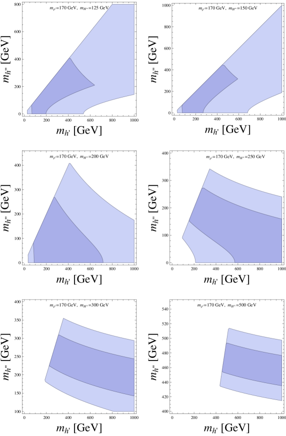
Figure 2: Same as in Fig. 1 but with the SM-like Higgs-boson mass fixed to $m_{\rho^{\prime}}=170$ GeV.

We shall now derive the predictions for the oblique parameters in the MCPM. In the MCPM the Yukawa couplings are completely fixed and the only free parameters we encounter in the calculation of the oblique parameters are the Higgs-boson masses $m_{\rho^{\prime}}$, $m_{h^{\prime}}$, $m_{h^{\prime\prime}}$, and $m_{H^{\pm}}$. Here $\rho^{\prime}$ and $h^{\prime}$ are the CP-even and $h^{\prime\prime}$ is the CP-odd Higgs boson and $H^{\pm}$ denotes the pair of charged Higgs bosons. In Figure 1 we show the contour plots for the 1-$\sigma$ (dark) and 2-$\sigma$ (bright) deviations of the oblique parameters from the electroweak precision data (42) in the $m_{h^{\prime}}$–$m_{h^{\prime\prime}}$ plane. The mass of the SM-like Higgs-boson $\rho^{\prime}$ is fixed to $m_{\rho^{\prime}}=$ 125 GeV. The charged-Higgs-boson mass $m_{H^{\pm}}$ is set to different values in the range of 125-500 GeV in the various plots. In Figure 2 we show analogous plots but for a mass of the SM-like Higgs boson $\rho^{\prime}$ of $m_{\rho^{\prime}}=$ 170 GeV. Note that we have always $m_{h^{\prime}}>m_{h^{\prime\prime}}$ in the MCPM which is the reason that there are no allowed regions of parameter space above the diagonal of equal masses $m_{h^{\prime}}=m_{h^{\prime\prime}}$ in Figures 1 and 2

We see from Figures 1 and 2 that there are large regions for the masses of the Higgs bosons $h^{\prime}$, $h^{\prime\prime}$, and $H^{\pm}$ where the electroweak constraints (42) are satisfied. The allowed regions for these masses, up to several hundred GeV, are very reasonable. The CP odd extra Higgs boson $h^{\prime\prime}$ could even be below 100 GeV in mass. But then it would be necessary to study all other experimental constraints for such a low-mass boson. Furthermore, we see from Figures 1 and 2 that with increasing masses of $\rho^{\prime}$ and $H^{\pm}$ also the allowed domains for the masses of the Higgs bosons $h^{\prime}$ and $h^{\prime\prime}$ shift to higher mass values.

VI Conclusions

In this paper we started with briefly reviewing the bilinear formalism which turns out to be quite powerful for the study of the THDM. We have discussed the classification of the possible symmetry classes without any assumption on the stability type of the THDM potential. We have given a practical and easily usable method how to determine the symmetry class of a given THDM Higgs potential. We have defined the symmetry classes to be mutually exclusive; see Table 1. We have also given the symmetry group $\mathbbm{G}$ corresponding to each symmetry class. We have focussed on one of these symmetry classes, denoted by CP2, in some detail. The CP2 symmetric THDM has a number of simultaneous CP invariances. As shown in Maniatis:2007de the extension of the CP symmetries of the potential to the Yukawa interactions leads in a straightforward way to the so-called maximally CP-symmetric model (MCPM). In this model the Yukawa couplings are completely fixed. We have studied the renormalisation-group equations of the quartic Higgs-potential parameters in this model. We have found that the symmetries of this model are preserved by the RGEs, as it has to be.

The MCPM has a hierarchy of quartic couplings $\mu_{1}>\mu_{2}>\mu_{3}$. We have shown that considering the theory of the Higgs bosons alone this hierarchy of quartic couplings turn out to be stable against renormalisation group evolution. However, taking the Yukawa couplings into account $\mu_{1}>\mu_{2}$ is stable but not necessarily $\mu_{2}>\mu_{3}$. Reaching $\mu_{2}=\mu_{3}$ at a certain renormalisation scale would elevate the CP2 symmetry of the Higgs potential to a CP3 symmetry. But, of course, this does not imply that the full MCPM which includes fermions and gauge bosons has a higher symmetry than CP2 at this renormalisation scale.

Eventually, we have computed the oblique parameters in the MCPM. We find for large parameter space agreement with the electroweak precision measurements. In particular we have presented the 1-$\sigma$ and 2-$\sigma$ contours of valid regions in the $m_{h^{\prime}}$–$m_{h^{\prime\prime}}$ mass plane for different choices for the charged-Higgs-boson mass and for SM-like Higgs-boson masses of 125 GeV and 170 GeV, respectively. The allowed regions for the masses of the Higgs bosons are in a reasonable range; see Figures 1 and 2. These Higgs bosons with masses below 500 GeV should therefore be detectable in the LHC experiments. As shown in Maniatis:2009vp ; Maniatis:2009by ; Maniatis:2010sb in the MCPM these Higgs bosons have characteristic production and decay properties giving clear experimental signatures.

Appendix A Derivation of symmetry classes

In this appendix we give a recipe which allows an easy identification of the symmetry class of any given THDM potential (8).

The first step is to diagonalise $E$ by a basis transformation (12). We get then

$$E=\operatorname{diag}(\mu_{1},\mu_{2},\mu_{3}).$$ (43)

Since $E$ is symmetric a diagonalisation is always possible. Therefore we work in the following in the $E$ diagonal basis and consider $\boldsymbol{\mathrm{\xi}}$ and $\boldsymbol{\mathrm{\eta}}$ (9) in this basis. Now we have to distinguish three cases for the $\mu$’s.

• $\mu_{1}$, $\mu_{2}$, $\mu_{3}$ all different.

  Then we see from (20) and (21) that only diagonal O(3) matrices $R$ or $\bar{R}$ may lead to symmetries, that is, we have to consider

  $$\begin{split}\bar{R}&=\bar{R}_{j}\quad(j=1,2,3;\quad\text{see}~{}\eqref{eqreflect}),\\ \bar{R}&=\bar{R}_{1}\bar{R}_{2}\bar{R}_{3}=-\mathbbm{1}_{3},\\ R&=\bar{R}_{i}\bar{R}_{j}\quad\text{with }i\neq j.\end{split}$$ (44)

  Now we can easily check the conditions for $\boldsymbol{\mathrm{\xi}}$, $\boldsymbol{\mathrm{\eta}}$ from (20) and (21). We can have the following cases:

  • $(\xi_{i},\eta_{i})\neq(0,0)\quad\text{for }i=1,2,3$.

    With none of the matrices from (44) we can fulfill the symmetry relations in (20). In this case the potential has only the trivial symmetry group $\mathbbm{G}=\{\mathbbm{1}_{3}\}$.

  • Exactly one pair fulfills $(\xi_{i},\eta_{i})=(0,0)$ where $i\in\{1,2,3\}$.

    Without loss of generality we can set $(\xi_{2},\eta_{2})=(0,0)$, $(\xi_{1},\eta_{1})\neq(0,0)$, $(\xi_{3},\eta_{3})\neq(0,0)$. Clearly, from (20), (21) we have $\bar{R}_{2}$ and nothing else as symmetry transformation. We get the symmetry group

    $$\mathbbm{G}=\{\mathbbm{1}_{3},\bar{R}_{2}\}$$ (45)

    which characterises the CP1 symmetry class; see Table 1, the first subclass of CP1.

  • Exactly two pairs fulfill $(\xi_{i},\eta_{i})=(0,0)$ where $i\in\{1,2,3\}$.

    Without loss of generality we can set $(\xi_{1},\eta_{1})=(\xi_{2},\eta_{2})=(0,0)$, $(\xi_{3},\eta_{3})\neq(0,0)$. From (20), (21) and (44) we see that the invariance group is

    $$\mathbbm{G}=\{\mathbbm{1}_{3},\bar{R}_{1},\bar{R}_{2},\bar{R}_{1}\bar{R}_{2}\}.$$ (46)

    We get the symmetry group characterising the $\mathbbm{Z}_{2}$ symmetry class; see Table 1, the first subclass of $\mathbbm{Z}_{2}$.

  • $\boldsymbol{\mathrm{\xi}}=0$ and $\boldsymbol{\mathrm{\eta}}=0$ .

    Here we find from (20), (21) and (44) as symmetry group

    $$\mathbbm{G}=\{\mathbbm{1}_{3},\bar{R}_{1},\bar{R}_{2},\bar{R}_{3},\bar{R}_{1}\bar{R}_{2},\bar{R}_{2}\bar{R}_{3},\bar{R}_{1}\bar{R}_{3},\bar{R}_{1}\bar{R}_{2}\bar{R}_{3}=-\mathbbm{1}_{3}\}.$$ (47)

    This characterises the CP2 symmetry class.

• Exactly two eigenvalues $\mu_{j}$ of $E$ are equal.

  Without loss of generality we set

  $$\mu_{1}=\mu_{2}\neq\mu_{3}.$$ (48)

  From  (20), (21) we see that $E$ allows now as invariances

  $$R_{2\theta} =\begin{pmatrix}\cos(2\theta)&-\sin(2\theta)&0\\ \sin(2\theta)&\cos(2\theta)&0\\ 0&0&1\end{pmatrix}\qquad 0\leq\theta<\pi,$$ (49)

  $$\bar{R} =\bar{R}_{j},\quad j=2,3,$$ (50)

  $$\bar{R} =R_{2\theta}\bar{R}_{3},$$ (51)

  $$\bar{R} =R_{2\theta}\bar{R}_{2}.$$ (52)

  Note that $\bar{R}_{1}$ is included in (52) for $2\theta=\pi$: $\bar{R}_{1}=R_{\pi}\bar{R}_{2}$.

  Now we consider again all possibilities for $\boldsymbol{\mathrm{\xi}}$ and $\boldsymbol{\mathrm{\eta}}$.

  • $(\xi_{3},\eta_{3})\neq(0,0)$ and $(\boldsymbol{\mathrm{\xi}}\times\boldsymbol{\mathrm{\eta}})\boldsymbol{\mathrm{e}}_{3}\neq 0$ .

    The first relation implies that neither $\bar{R}_{3}$ (50) nor any $R_{2\theta}\bar{R}_{3}$ (51) can lead to a symmetry. The second relation implies that $(\xi_{1},\xi_{2})^{\mathrm{T}}$ and $(\eta_{1},\eta_{2})^{\mathrm{T}}$ are linearly independent. Therefore, neither $R_{2\theta}$ (49) nor any $R_{2\theta}\bar{R}_{2}$ (52) can lead to a symmetry and we have here only the trivial invariance group

    $$\mathbbm{G}=\{\mathbbm{1}_{3}\}.$$ (53)

  • $(\xi_{3},\eta_{3})\neq(0,0)$, $(\boldsymbol{\mathrm{\xi}}\times\boldsymbol{\mathrm{\eta}})\boldsymbol{\mathrm{e}}_{3}=0$, $(\boldsymbol{\mathrm{\xi}}-\xi_{3}\boldsymbol{\mathrm{e}}_{3},\boldsymbol{\mathrm{\eta}}-\eta_{3}\boldsymbol{\mathrm{e}}_{3})\neq(0,0)$.

    Here the vectors $(\xi_{1},\xi_{2})^{\mathrm{T}}$ and $(\eta_{1},\eta_{2})^{\mathrm{T}}$ are linearly dependent but at least one of them is non zero. Due to $\mu_{1}=\mu_{2}\neq\mu_{3}$, see (48), we can make a basis change in the 1–2 subspace and achieve, without loss of generality, $(\xi_{1},\eta_{1})\neq(0,0)$ and $(\xi_{2},\eta_{2})=(0,0)$. We see now that here from all possible invariances (49) to (52) only $\bar{R}_{2}$ remains. Thus, the invariance group is

    $$\mathbbm{G}=\{\mathbbm{1}_{3},\bar{R}_{2}\}$$ (54)

    and we get the CP1 class. This is the third subclass of CP1 listed in Table 1.

  • $(\xi_{3},\eta_{3})\neq(0,0)$, $(\boldsymbol{\mathrm{\xi}}\times\boldsymbol{\mathrm{\eta}})\boldsymbol{\mathrm{e}}_{3}=0$, $(\boldsymbol{\mathrm{\xi}}-\xi_{3}\boldsymbol{\mathrm{e}}_{3},\boldsymbol{\mathrm{\eta}}-\eta_{3}\boldsymbol{\mathrm{e}}_{3})=(0,0)$.

    This case can also be characterised by

    $$\boldsymbol{\mathrm{\xi}}\times\boldsymbol{\mathrm{e}}_{3}=0,\quad\boldsymbol{\mathrm{\eta}}\times\boldsymbol{\mathrm{e}}_{3}=0,\quad(\boldsymbol{\mathrm{\xi}},\boldsymbol{\mathrm{\eta}})\neq(0,0).$$ (55)

    That is, we have here

    $$\boldsymbol{\mathrm{\xi}}=\begin{pmatrix}0\\ 0\\ \xi_{3}\end{pmatrix},\quad\boldsymbol{\mathrm{\eta}}=\begin{pmatrix}0\\ 0\\ \eta_{3}\end{pmatrix},\quad(\xi_{3},\eta_{3})\neq(0,0).$$ (56)

    From (49) to (52) we see that in this case the invariance group is

    $$\mathbbm{G}=\{R_{2\theta},R_{2\theta}\bar{R}_{2}\}.$$ (57)

    We get the first subclass of the U(1) symmetry class in Table 1.

  • $(\xi_{3},\eta_{3})=(0,0)$, $\boldsymbol{\mathrm{\xi}}\times\boldsymbol{\mathrm{\eta}}\neq 0$ .

    Here $(\xi_{1},\xi_{2})^{\mathrm{T}}$ and $(\eta_{1},\eta_{2})^{\mathrm{T}}$ are linearly independent. We see from (20) and (21) that neither $R_{2\theta}$ ($0<\theta<\pi$) nor $R_{2\theta}\bar{R}_{2}$ ($0\leq\theta<\pi$) can lead to invariances. But, clearly, $\bar{R}_{3}$ gives an invariance and the corresponding symmetry group is

    $$\mathbbm{G}=\{\mathbbm{1}_{3},\bar{R}_{3}\}.$$ (58)

    This group is, of course, equivalent to $\mathbbm{G}=\{\mathbbm{1}_{3},\bar{R}_{2}\}$ as we see after a trivial exchange of numbering of the 2 and the 3 axes. We list this case as second subclass of the CP1 class in Table 1.

  • $(\xi_{3},\eta_{3})=(0,0)$, $\boldsymbol{\mathrm{\xi}}\times\boldsymbol{\mathrm{\eta}}=0$, $(\boldsymbol{\mathrm{\xi}},\boldsymbol{\mathrm{\eta}})\neq(0,0)$.

    Here $(\xi_{1},\xi_{2})^{\mathrm{T}}$ and $(\eta_{1},\eta_{2})^{\mathrm{T}}$ are linearly dependent. We can make a rotation in the 1–2 subspace to achieve $(\xi_{1},\eta_{1})\neq(0,0)$ and $(\xi_{2},\eta_{2})=(0,0)$. From (20), (21) and (49) to (52) we see that here the symmetry group is

    $$\mathbbm{G}=\{\mathbbm{1}_{3},\bar{R}_{2},\bar{R}_{3},\bar{R}_{2}\bar{R}_{3}\}.$$ (59)

    After an exchange of numbering of the 1 and 3 axes this gives the second subclass of the $\mathbbm{Z}_{2}$ class in Table 1.

  • $\boldsymbol{\mathrm{\xi}}=0$, $\boldsymbol{\mathrm{\eta}}=0$.

    Here we have invariance for all the transformations (49) to (52). The corresponding symmetry group is

    $$\mathbbm{G}=\{R_{2\theta},R_{2\theta}\bar{R}_{2},R_{2\theta}\bar{R}_{3}\}\quad\text{with }0\leq\theta<\pi.$$ (60)

    We get the CP3 class.

• $\mu_{1}=\mu_{2}=\mu_{3}\equiv\mu$.

  Here we have $E=\mu\mathbbm{1}_{3}$ and $E$ allows as invariance all $R$ and $\bar{R}$ matrices of O(3). We distinguish the following subcases.

  • $\boldsymbol{\mathrm{\xi}}\times\boldsymbol{\mathrm{\eta}}\neq 0$.

    Without loss of generality we choose the second axis to be parallel to $\boldsymbol{\mathrm{\xi}}\times\boldsymbol{\mathrm{\eta}}$. We have then $(\xi_{2},\eta_{2})=(0,0)$ and further that $(\xi_{1},\xi_{3})^{\mathrm{T}}$ and $(\eta_{1},\eta_{3})^{\mathrm{T}}$ are linearly independent. The invariance group is

    $$\mathbbm{G}=\{\mathbbm{1}_{3},\bar{R}_{2}\}$$ (61)

    and we get the fourth subclass of the CP1 class in Table 1.

  • $\boldsymbol{\mathrm{\xi}}\times\boldsymbol{\mathrm{\eta}}=0$, $(\boldsymbol{\mathrm{\xi}},\boldsymbol{\mathrm{\eta}})\neq(0,0)$.

    Here the vectors $\boldsymbol{\mathrm{\xi}}$ and $\boldsymbol{\mathrm{\eta}}$ are parallel and at least one of them is unequal zero. We choose this vector to define the 3 axis and get

    $$\boldsymbol{\mathrm{\xi}}=\begin{pmatrix}0\\ 0\\ \xi_{3}\end{pmatrix},\quad\boldsymbol{\mathrm{\eta}}=\begin{pmatrix}0\\ 0\\ \eta_{3}\end{pmatrix},\quad\text{with }(\xi_{3},\eta_{3})\neq(0,0).$$ (62)

    The invariance group is then from (20) and (21)

    $$\mathbbm{G}=\{R_{2\theta},R_{2\theta}\bar{R}_{2}\};$$ (63)

    see (49) to (52). We get the second subclass of the U(1) class in Table 1.

  • $\boldsymbol{\mathrm{\xi}}=0$, $\boldsymbol{\mathrm{\eta}}=0$.

    Here, clearly, we get as symmetry group

    $$\mathbbm{G}=\text{O(3)}=\{R,R\bar{R}_{2}\},\quad\text{with }R\in\text{SO(3)}.$$ (64)

    This is labeled as SO(3) class in Table 1.

To summarize, in this appendix we have – in a systematic way – gone through all possibilities for the potential parameters $E$, $\boldsymbol{\mathrm{\xi}}$, $\boldsymbol{\mathrm{\eta}}$ and checked for possible symmetry groups. For any given THDM potential all these steps are easily done and this gives a practical way to identify if any and what symmetry the potential has. Of course, a symmetry of the potential is not guaranteed to be respected by the Yukawa couplings. This has to be checked as a second step. Such a program has, for instance, be carried through for the MCPM in Maniatis:2007de .

The corespondence of the Higgs-family transformations for fields and field bilinears is given in (11) resp. (12). An $R$ in (12) determines $U$ in (11) up to gauge transformations. Similarly, for GCP transformations $\bar{R}$ in (16) determines $U$ in (15) up to gauge transformations. In Tables 2 and 3 we give these correspondences of transformations in field and $K$ space for the elements of the groups $\mathbbm{G}$ occuring in Table 1.

$R$	$U$
$\bar{R}_{1}\bar{R}_{2}=\operatorname{diag}(-1,-1,1)$	$\sigma^{3}$
$\bar{R}_{2}\bar{R}_{3}=\operatorname{diag}(1,-1,-1)$	$\sigma^{1}$
$\bar{R}_{1}\bar{R}_{3}=\operatorname{diag}(-1,1,-1)$	$\sigma^{2}$
$R_{2\theta}$, see (49) and (14) with $\alpha=2\theta$	$\cos(\theta)\mathbbm{1}_{2}-i\sin(\theta)\sigma^{3}$

Table 2: Correspondence of proper rotation matrices $R$ in (12) and field transformations $U$ in (11).

$\bar{R}$	$U$
$\bar{R}_{1}=\operatorname{diag}(-1,1,1)$	$\sigma^{3}$
$\bar{R}_{2}=\operatorname{diag}(1,-1,1)$	$\mathbbm{1}_{2}$
$\bar{R}_{3}=\operatorname{diag}(1,1,-1)$	$\sigma^{1}$
$-\mathbbm{1}_{3}$	$\epsilon=i\sigma^{2}$
$R_{2\theta}\bar{R}_{2}$, see (52)	$\cos(\theta)\mathbbm{1}_{2}-i\sin(\theta)\sigma^{3}$
$R_{2\theta}\bar{R}_{3}$, see (51)	$\cos(\theta)\sigma^{1}+\sin(\theta)\sigma^{2}$

Table 3: Correspondence of improper rotation matrices $\bar{R}$ in (16) and matrices $U$ in GCP transformations of fields (15).

Appendix B Lagrangian of the MCPM

In sections IV and V we consider a model corresponding to the symmetry class CP2 in Table 1, the MCPM. Here we recall the Lagrangian of this model as originally given in Maniatis:2007de .

The Lagrangian of the MCPM can be written as

$$\mathscr{L}_{\text{MCPM}}=\mathscr{L}_{\varphi}+\mathscr{L}_{\text{Yuk}}+\mathscr{L}_{\text{FB}}\,.$$ (65)

Here $\mathscr{L}_{\text{FB}}$ is the standard gauge kinetic Lagrange density for fermions and gauge bosons (see for instance Nachtmann:1990ta ).

The Higgs-boson Lagrangian is

$$\mathscr{L}_{\varphi}=\sum_{i=1,2}\left(D_{\mu}\varphi_{i}\right)^{\dagger}\left(D^{\mu}\varphi_{i}\right)-V(\varphi_{1},\varphi_{2})\,,$$ (66)

with $V(\varphi_{1},\varphi_{2})$ the Higgs potential (8) with the constraints (22). The covariant derivative reads

$$D_{\mu}=\partial_{\mu}+ig_{2}W_{\mu}^{a}{\bf T}_{a}+ig_{1}B_{\mu}{\bf Y}$$ (67)

where ${\bf T}_{a}$ and ${\bf Y}$ are the generating operators of weak-isospin and weak-hypercharge transformations, respectively. $W_{\mu}^{a}$, $a=1,2,3$ and $B_{\mu}$ are the gauge fields and $g_{2}$ and $g_{1}$ the corresponding gauge couplings. For the Higgs doublets we have ${\bf T}_{a}=\sigma^{a}/2$ where $\sigma^{a}$ with $a=1,2,3$ are the Pauli matrices. We choose the convention that both Higgs-boson doublets have weak hypercharge $y=+1/2$.

Furthermore, $\mathscr{L}_{\text{Yuk}}$ denotes the Yukawa term which in the MCPM has the form

$$\begin{split}\mathscr{L}_{\mathrm{Yuk}}(x)=-c_{\tau}&\;\Bigg{[}\bar{\tau}_{R}(x)\,\varphi_{1}^{\dagger}(x)\begin{pmatrix}\nu_{\tau\,L}(x)\\ \tau_{L}(x)\end{pmatrix}\;-\bar{\mu}_{R}(x)\,\varphi_{2}^{\dagger}(x)\begin{pmatrix}\nu_{\mu\,L}(x)\\ \mu_{L}(x)\end{pmatrix}\Bigg{]}\\ +c_{t}&\;\Bigg{[}\bar{t}_{R}(x)\,\varphi_{1}^{\mathrm{T}}(x)\,\epsilon\begin{pmatrix}t_{L}(x)\\ b_{L}(x)\end{pmatrix}\;-\bar{c}_{R}(x)\,\varphi_{2}^{\mathrm{T}}(x)\,\epsilon\begin{pmatrix}c_{L}(x)\\ s_{L}(x)\end{pmatrix}\Bigg{]}\\ -c_{b}&\;\Bigg{[}\bar{b}_{R}(x)\,\varphi_{1}^{\dagger}(x)\begin{pmatrix}t_{L}(x)\\ b_{L}(x)\end{pmatrix}\;-\bar{s}_{R}(x)\,\varphi_{2}^{\dagger}(x)\begin{pmatrix}c_{L}(x)\\ s_{L}(x)\end{pmatrix}\Bigg{]}+h.c.\end{split}$$ (68)

where $\epsilon=i\sigma^{2}$ and $c_{\tau}$, $c_{t}$ and $c_{b}$ are real positive constants, determined by the vacuum expectation value $v_{0}$ and the fermion masses; see (31). Note that the first family remains uncoupled – at tree level – to the Higgs bosons in the MCPM.

Through EWSB only the Higgs-boson doublet $\varphi_{1}$ gets a vacuum-expectation value. In the unitary gauge we have

$$\varphi_{1}(x)=\frac{1}{\sqrt{2}}\begin{pmatrix}0\\ v_{0}+\rho^{\prime}(x)\end{pmatrix},\qquad\varphi_{2}(x)=\begin{pmatrix}H^{+}(x)\\ \frac{1}{\sqrt{2}}(h^{\prime}(x)+ih^{\prime\prime}(x))\end{pmatrix},$$ (69)

where $\rho^{\prime}(x)$, $h^{\prime}(x)$ and $h^{\prime\prime}(x)$ are the real fields corresponding to the physical neutral Higgs particles. The fields $H^{+}(x)$ and $H^{-}(x)=\big{(}H^{+}(x)\big{)}^{\dagger}$ correspond to the physical charged Higgs-boson pair.

References

• (1) P. Fayet, “A Gauge Theory of Weak and Electromagnetic Interactions with Spontaneous Parity Breaking,” Nucl. Phys.  B78, 14 (1974).
• (2) P. Fayet, “Supergauge Invariant Extension of the Higgs Mechanism and a Model for the electron and Its Neutrino,” Nucl. Phys.  B90, 104-124 (1975).
• (3) K. Inoue, A. Kakuto, H. Komatsu, S. Takeshita, “Aspects of Grand Unified Models with Softly Broken Supersymmetry,” Prog. Theor. Phys.  68 927 (1982).
• (4) K. Inoue, A. Kakuto, H. Komatsu, S. Takeshita, “Renormalization of Supersymmetry Breaking Parameters Revisited,” Prog. Theor. Phys.  71, 413 (1984).
• (5) R. A. Flores, M. Sher, “Higgs Masses in the Standard, Multi-Higgs and Supersymmetric Models,” Annals Phys.  148, 95 (1983).
• (6) J. F. Gunion, H. E. Haber, “Higgs Bosons in Supersymmetric Models. 1.,” Nucl. Phys.  B272, 1 (1986).
• (7) R.D. Peccei and H.R. Quinn, “CP Conservation in the Presence of Instantons,” Phys. Rev. Lett.  38, 1440 (1977).
• (8) R.D. Peccei and H.R. Quinn, “Constraints Imposed by CP Conservation in the Presence of Instantons,” Phys. Rev.  D 16, 1791 (1977).
• (9) T. D. Lee, “A Theory of Spontaneous T Violation,” Phys. Rev.  D 8, 1226 (1973).
• (10) N. G. Deshpande, E. Ma, “Pattern of Symmetry Breaking with Two Higgs Doublets,” Phys. Rev.  D18, 2574 (1978).
• (11) H. Georgi, “A Model of Soft CP Violation,” Hadronic J.  1, 155 (1978).
• (12) H. E. Haber, G. L. Kane, T. Sterling, “The Fermion Mass Scale and Possible Effects of Higgs Bosons on Experimental Observables,” Nucl. Phys.  B161, 493 (1979).
• (13) J. F. Donoghue, L. F. Li, “Properties of Charged Higgs Bosons,” Phys. Rev.  D19, 945 (1979).
• (14) E. Golowich, T. C. Yang, “Charged Higgs Bosons And Decays Of Heavy Flavored Mesons,” Phys. Lett.  B80, 245 (1979).
• (15) L. J. Hall, M. B. Wise, “Flavor Changing Higgs - Boson Couplings,” Nucl. Phys.  B187, 397 (1981).
• (16) H. E. Haber, R. Hempfling, “The Renormalization group improved Higgs sector of the minimal supersymmetric model,” Phys. Rev.  D48, 4280-4309 (1993) [hep-ph/9307201].
• (17) G. Cvetic, “CP violation in bosonic sector of SM with two Higgs doublets,” Phys. Rev.  D48, 5280-5285 (1993) [hep-ph/9309202].
• (18) F. J. Botella, J. P. Silva, “Jarlskog - like invariants for theories with scalars and fermions,” Phys. Rev.  D51, 3870-3875 (1995) [hep-ph/9411288].
• (19) L. Lavoura, J. P. Silva, “Fundamental CP violating quantities in a SU(2) x U(1) model with many Higgs doublets,” Phys. Rev.  D50, 4619-4624 (1994) [hep-ph/9404276].
• (20) L. Lavoura, “Signatures of discrete symmetries in the scalar sector,” Phys. Rev.  D50, 7089-7092 (1994) [hep-ph/9405307].
• (21) J. Velhinho, R. Santos and A. Barroso, “Tree level vacuum stability in two-Higgs doublet models,” Phys. Lett.  B 322, 213 (1994).
• (22) W. Bernreuther, O. Nachtmann, “Flavor dynamics with general scalar fields,” Eur. Phys. J.  C9, 319-333 (1999) [hep-ph/9812259].
• (23) I. F. Ginzburg, M. Krawczyk, “Symmetries of two Higgs doublet model and CP violation,” Phys. Rev.  D72, 115013 (2005) [hep-ph/0408011].
• (24) R. Barbieri and L. J. Hall, “Improved naturalness and the two Higgs doublet model”, [hep-ph/0510243].
• (25) S. Davidson, H. E. Haber, “Basis-independent methods for the two-Higgs-doublet model,” Phys. Rev.  D72, 035004 (2005) [hep-ph/0504050].
• (26) F. Nagel, “New aspects of gauge-boson couplings and the Higgs sector”, Ph. D. thesis (University of Heidelberg, 2004), available from http://www.slac.stanford.edu/spires/find/hep/www?irn=6461018 or http://www.ub.uni-heidelberg.de/archiv/4803.
• (27) M. Maniatis, A. von Manteuffel, O. Nachtmann and F. Nagel, “Stability and symmetry breaking in the general two-Higgs-doublet model,” Eur. Phys. J.  C 48, 805 (2006) [hep-ph/0605184].
• (28) C. C. Nishi, “CP violation conditions in N-Higgs-doublet potentials,” Phys. Rev.  D 74 036003 (2006) [hep-ph/0605153].
• (29) I. P. Ivanov, “Minkowski space structure of the Higgs potential in 2HDM,” Phys. Rev.  D 75 035001 (2007) [hep-ph/0609018].
• (30) M. Maniatis, A. von Manteuffel and O. Nachtmann, “CP Violation in the General Two-Higgs-Doublet Model: a Geometric View,” Eur. Phys. J.  C 57, 719 (2008) [0707.3344 [hep-ph]].
• (31) P. M. Ferreira, H. E. Haber and J. P. Silva, “Generalized CP symmetries and special regions of parameter space in the two-Higgs-doublet model,” Phys. Rev.  D 79, 116004 (2009) [0902.1537 [hep-ph]].
• (32) F. Mahmoudi, O. Stal, “Flavor constraints on the two-Higgs-doublet model with general Yukawa couplings,” Phys. Rev.  D81, 035016 (2010) [0907.1791 [hep-ph]].
• (33) B. Grzadkowski, M. Maniatis and J. Wudka, “Note on Custodial Symmetry in the Two-Higgs-Doublet Model,” 1011.5228 [hep-ph].
• (34) M. Maniatis, A. von Manteuffel and O. Nachtmann, “A new type of CP symmetry, family replication and fermion mass hierarchies,” Eur. Phys. J.  C 57, 739 (2008) [0711.3760 [hep-ph]].
• (35) M. Maniatis, O. Nachtmann, “On the phenomenology of a two-Higgs-doublet model with maximal CP symmetry at the LHC,” JHEP 0905, 028 (2009) [0901.4341 [hep-ph]].
• (36) M. Maniatis, O. Nachtmann, “On the phenomenology of a two-Higgs-doublet model with maximal CP symmetry at the LHC. II. Radiative effects,” JHEP 1004, 027 (2010) [0912.2727 [hep-ph]].
• (37) M. Maniatis, O. Nachtmann, A. von Manteuffel, “On the phenomenology of a two-Higgs-doublet model with maximal CP symmetry at the LHC: Synopsis and addendum,” DESY-PROC-2010-001 [1009.1869 [hep-ph]].
• (38) I. P. Ivanov, “Minkowski space structure of the Higgs potential in 2HDM. II. Minima, symmetries, and topology,” Phys. Rev.  D77, 015017 (2008) [0710.3490 [hep-ph]].
• (39) E. Ma, M. Maniatis, “Symbiotic Symmetries of the Two-Higgs-Doublet Model,” Phys. Lett.  B683, 33-38 (2010) [0909.2855 [hep-ph]].
• (40) P. M. Ferreira, M. Maniatis, O. Nachtmann, J. P. Silva, “CP properties of symmetry-constrained two-Higgs-doublet models,” JHEP 1008, 125 (2010) [1004.3207 [hep-ph]].
• (41) P. M. Ferreira, H. E. Haber, M. Maniatis, O. Nachtmann, J. P. Silva, “Geometric picture of generalized-CP and Higgs-family transformations in the two-Higgs-doublet model,” Int. J. Mod. Phys.  A26, 769-808 (2011) [1010.0935 [hep-ph]].
• (42) M. E. Peskin, T. Takeuchi, “A New constraint on a strongly interacting Higgs sector,” Phys. Rev. Lett.  65, 964-967 (1990).
• (43) T. D. Lee and G. C. Wick, “Space inversion, time reversal, and other discrete symmetries in local field theories”, Phys. Rev.  148, 1385 (1966).
• (44) G. Ecker, W. Grimus and W. Konetschny, “Quark Mass Matrices In Left-Right Symmetric Gauge Theories,” Nucl. Phys.  B 191 (1981) 465.
• (45) G. Ecker, W. Grimus and H. Neufeld, “Spontaneous CP Violation In Left-Right Symmetric Gauge Theories,” Nucl. Phys.  B 247 70 (1984) .
• (46) J. Bernabeu, G. C. Branco and M. Gronau, “CP Restrictions On Quark Mass Matrices,” Phys. Lett.  B 169, 243 (1986).
• (47) G. Ecker, W. Grimus and H. Neufeld, “A Standard Form For Generalized CP Transformations,” J. Phys. A 20 L807 (1987).
• (48) H. Neufeld, W. Grimus and G. Ecker, “Generalized CP invariance, neutral flavor conservation and the structure of the mixing matrix”, Int. J. Mod. Phys.  A 3 603 (1988).
• (49) T. P. Cheng, E. Eichten, L. -F. Li, “Higgs Phenomena in Asymptotically Free Gauge Theories,” Phys. Rev.  D9, 2259 (1974).
• (50) K.Nakamura et al. [ Particle Data Group Collaboration ], “Review of particle physics,” J. Phys. G G37, 075021 (2010).
• (51) C. D. Froggatt, R. G. Moorhouse, I. G. Knowles, “Leading radiative corrections in two scalar doublet models,” Phys. Rev.  D45, 2471-2481 (1992).
• (52) H. E. Haber, D. O’Neil, “Basis-independent methods for the two-Higgs-doublet model III: The CP-conserving limit, custodial symmetry, and the oblique parameters S, T, U,” 1011.6188 [hep-ph].
• (53) O. Nachtmann, “Elementary Particle Physics: Concepts And Phenomena”, Springer, Berlin (1990).