Financial factor influence on scaling and memory of trading volume in stock market

Abstract

We study the daily trading volume volatility of 17,197 stocks in the U.S. stock markets during the period 1989–2008 and analyze the time return intervals $\tau$ between volume volatilities above a given threshold $q$. For different thresholds $q$, the probability density function $P_{q}(\tau)$ scales with mean interval $\langle\tau\rangle$ as $P_{q}(\tau)=\langle\tau\rangle^{-1}f(\tau/\langle\tau\rangle)$ and the tails of the scaling function can be well approximated by a power-law $f(x)\sim x^{-\gamma}$. We also study the relation between the form of the distribution function $P_{q}(\tau)$ and several financial factors: stock lifetime, market capitalization, volume, and trading value. We find a systematic tendency of $P_{q}(\tau)$ associated with these factors, suggesting a multi-scaling feature in the volume return intervals. We analyze the conditional probability $P_{q}(\tau|\tau_{0})$ for $\tau$ following a certain interval $\tau_{0}$, and find that $P_{q}(\tau|\tau_{0})$ depends on $\tau_{0}$ such that immediately following a short/long return interval a second short/long return interval tends to occur. We also find indications that there is a long-term correlation in the daily volume volatility. We compare our results to those found earlier for price volatility.

I Introduction

Because the dynamics of financial markets are of great importance in economics and econophysics Mandelbrot63 ; Mantegna95 ; Kondor99 ; Mantegna00 ; Takayasu97 ; Bouchaud00 ; Johnson03 ; Liu99 ; Plerou01 , the dynamics of both stock price and trading volume have been studied for decades as a prerequisite to developing effective investment strategies. Econophysics research has found that the distribution of stock price returns exhibits power-law tails and that the price volatility time series has long-term power-law correlations Engle93 ; Ord85 ; Harris86 ; Pfleiderer88 ; Schwert ; Pictet93 ; Pagan96 ; Ding96 ; Liu97 ; Cont98 ; Cizeau97 ; Pasquini99 . To better understand these scaling features and correlations, Yamasaki et al. Yamasaki05 and Wang et al. Wang06 ; Wang07 studied the behavior of price return intervals $\tau$ between volatilities occurring above a given threshold $q$. For both daily and intraday financial records, they found that (i) the distribution of the scaled price interval $\tau/\langle\tau\rangle$ can be approximated by a stretched exponential function, and (ii) the sequence of the price return intervals has a long term memory related to the original volatility sequence. The scaling and memory properties of financial records are similar to those found in climate and earthquake data Bunde04 ; Bunde05 ; Livina05 ; Lennartz08 ; Altmann05 ; Lux96 .

A feature of the recent history of the stock market has been large price movements associated with high volume. In the Black Monday stock market crash of 1987, the Dow Jones Industrials Average (DJIA) plummeted 508 points, losing 22.6 percent of its value in one day, which led to the pathological situation in which the bid price for a stock actually exceeded the ask price. In this financial crash approximately $6\times 10^{8}$ shares traded, a one-day trading volume three times that of the entire week previous. Understanding the precise relationship between price and volume fluctuations has thus been a topic of great interest in recent research Plerou00 ; Gopikrishnan00 . Trading volume data in itself contains much information about market dynamics, e.g., the distribution of the daily traded volume displays power-law tails with an exponent within the Lévy stable domain Plerou07 ; Plerou09 . Recently, Ren and Zhou Ren10 studied the intraday database of two composite indices and 20 individual indices in the Chinese stock markets. They found that the intraday volume recurrence intervals show a power-law scaling, short-term correlations and long-term correlations in each stock index.

In this study we analyze U.S. stock market data over a range broad enough to allow us to identify how several financial factors significantly affect scaling properties. We study the daily trading volume volatility return intervals $\tau$ between two successive volume volatilities above a certain threshold $q$, and find a range of power-law distributions broader than that found earlier in price volatility return intervals Yamasaki05 ; Wang06 . We find a unique scaling of the probability density function (PDF) $P_{q}(\tau)$ for different thresholds $q$. We also perform a detailed analysis of the relation between volume volatility return intervals and four financial stock factors: (i) stock lifetime, (ii) market capitalization, (iii) average trading volume, and (iv) average trading value. We find systematically different power-law exponents for $P_{q}(\tau)$ when binning stocks according to these four financial factors. Similar to that found for the Chinese market Ren10 , we find that in the U.S. stock market the conditional probability distribution, $P_{q}(\tau|\tau_{0})$ for $\tau$ following a certain interval $\tau_{0}$, demonstrates that volume return intervals are short-term correlated. We also find that the daily volume volatility shows a stronger long-term correlation for sequences of longer lifetime but no clear changes in long-term correlations for different stock size factors such as capitalization, volume, and trading value.

II Data

In order to obtain a sufficiently long time series, we analyze the daily trading volume volatility of 17,197 stocks listed in the U.S. stock market for at least 350 days. We obtain our data from the Center for Research in Security Prices (CRSP) US stock database, which lists the daily prices of all listed NYSE, Amex, and NASDAQ common stocks, along with basic market indices. The period we study extends from 1 January 1989 to 31 December 2008, a total of 5042 trading days.

III Distribution of Volume Volatility Return Intervals

For a stock trading volume time series, in a manner similar to stock price analysis Cizeau97 ; Pasquini99 ; Wang06 , we define two basic measures: volume return $R$ and volume volatility $\nu$. The volume return $R$ is defined as the logarithmic change in the successive daily trading volume for each stock,

$$R(t)\equiv\ln\left(\frac{V(t)}{V(t-1)}\right),$$ (1)

where $V(t)$ is the daily trading volume at time $t$. We define volume volatility to be the absolute value of the volume return. In order to compare different stocks, we determine the volume volatility $\nu(t)$ by dividing the absolute returns $|R(t)|$ by their standard deviation,

$$\nu(t)\equiv\ \frac{|R(t)|}{(\langle|R(t)|^{2}\rangle-{\langle|R(t)|\rangle}^{2})^{1/2}},$$ (2)

where $\langle\cdots\rangle$ is the time average for each stock. The threshold $q$ is thus measured in units of standard deviation of absolute volume return $|R(t)|$.

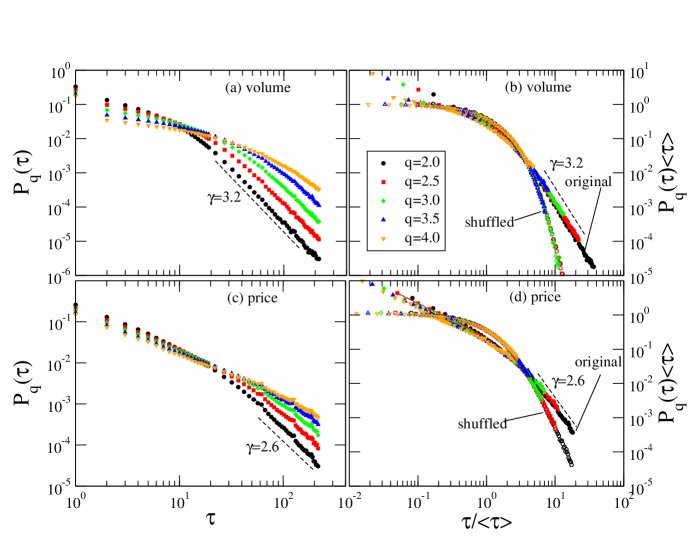
Figure 1: (Color online) Probability distributions of volume volatility return intervals and price volatility return intervals for 17197 stocks. Full symbols with different shapes represent different thresholds $q$ varying from 2.0 to 4.0. (a) Distribution of volume volatility return intervals, $P_{q}(\tau)$ versus $\tau$. (b) Scaled distribution of volume return intervals (full symbols) $P_{q}(\tau)\langle\tau\rangle$ versus $\tau/\langle\tau\rangle$, and distribution of volume return intervals for shuffled volatility records (open symbols). The four curves with full symbols collapse onto one single curve, indicating a universal scaling function. The tail of scaling function is approximately power-law distribution, $f(x)\sim x^{-\gamma}$, with $\gamma\cong 3.2$, while the curve fitting the shuffled records is exponential function, $f(x)=e^{-ax}$, from Possion distribution. A Poisson distribution indicates no correlation in shuffled volatility data, but the original dataset suggests strong correlation in the volatilities. The power-law exponents for intraday volume recurrence intervals of several Chinese stock indices are from $\gamma=1.71$ to $\gamma=3.27$ Ren10 . For comparison, (c) and (d) show the distribution and scaled distribution of price volatility return intervals respectively. Note the narrow range of power-law compared to (a).

For a volume volatility time series, we collect the time intervals $\tau$ between consecutive volatilities $\nu(t)$ above a chosen threshold $q$ and construct a new time series of volume return intervals $\{\tau(q)\}$. Fig. 1(a) shows the dependence of $P_{q}(\tau)$ on $q$, where $P_{q}(\tau)$ is the PDF of the volume volatility return interval time series $\{\tau(q)\}$. Obviously, $P_{q}(\tau)$ decays more slowly for large $q$ than for small $q$. For large $q$, $P_{q}(\tau)$ has a higher probability of having large interval values because extreme events are rare in a high threshold series. We next determine whether there is there any scaling in the distribution by plotting the PDFs of the volume return intervals $P_{q}(\tau)$, scaled with the mean volume return interval $\langle\tau(q)\rangle$, for different thresholds in Fig. 1(b). We can see that all five threshold values $q$ curves (full symbols) callapse onto a single curve, suggesting the existence of a scaling relation,

$$P_{q}(\tau)=\frac{1}{\langle\tau\rangle}f\left(\frac{\tau}{\langle\tau\rangle}\right).$$ (3)

As the threshold $q$ increases, the curve (rare events) tends to be truncated due to the limited size of the dataset. The tails of the scaling function can be approximated by a power-law function as shown by the dashed line in Fig. 1(b),

$$f\left(\frac{\tau}{\langle\tau\rangle}\right)\sim{\left(\frac{\tau}{\langle\tau\rangle}\right)}^{-\gamma},$$ (4)

where the tail exponent is $\gamma$. The exponent of the scaled PDFs for $q=2$ is $\gamma\cong 3.2$ by the least square method, which is the same as the unscaled PDF exponent $\gamma\cong 3.2$ as shown in Fig. 1(a). The power-law exponents for intraday volume recurrence intervals of several Chinese stock indices are from $\gamma=1.71$ to $\gamma=3.27$ Ren10 . Our exponents $\gamma$ are larger than those in the Chinese stock markets. This might be due to differing definitions of volume volatility. In Ref. Ren10 , the volume volatility is defined as intraday volume divided by the average volume at one specific minute of the trading day averaged over all trading days. Here we define the volume volatility to be the logarithmic change in the successive daily volumes [Eqs. 1 and  2]. For comparison, and using the same approach, Fig. 1(c) and Fig. 1(d) show the analogous results for price volatilities (see also the studies in Refs. Yamasaki05 ; Wang06 ; Jung08 ). Note that it is not easy to distinguish between a stretched exponential and a power-law when studying price volatilities Yamasaki05 , i.e., the power-law range is small and a stretched exponential could also provide a good fit. In contrast, the PDFs of the volume volatility return intervals display a wide range of power-law tails, which differs from the stretched exponential tail apparent in the price return intervals Wang06 . Our results for volume volatility may suggest that $P_{q}(\tau)$ for price volatility is also a power-law, but this could not be verified because the range of the observed power-law regime [see Figs. 1(c) and 1(d)] is more limited than the broad range of scales seen in the volume volatility [Figs. 1(a) and 1(b)]. The difference between the power-law and stretched exponential behavior of $P_{q}(\tau)$ may be related to the existence or non-existence respectively of non-linearity represented in the multifractality of the time series. When non-linear correlations appear in a time record, Bugachev et al. Bogachev07 showed that $P_{q}(\tau)$ is a power-law. On the other hand, when non-linear correlations do not exist and only linear correlation exists, Bunde et al. Bunde05 found stretched exponential behavior.

A comparison with the shuffled records allows us to see how the empirical records differ from randomized records. We shuffle the volume volatility time series to make a new uncorrelated sequence of volatility, and then collect the time intervals above a given threshold $q$ to obtain synthetic random control records. The curve that fits the shuffled records [the open symbols in Fig. 1(b)] is an exponential function, $f(x)=e^{-ax}$, and forms a Possion distribution. A Poisson distribution indicates no correlation in shuffled volatility data, but the empirical records suggest strong correlations in the volatility.

IV financial factors

We study the relation between the scaled PDFs $P_{q}(\tau)\langle\tau\rangle$ as a function of $\tau/\langle\tau\rangle$ for four financial factors: (a) stock lifetime, (b) market capitalization, (c) mean volume, and (d) mean trading value for threshold $q=2.0$. For higher $q$ values, we do not have sufficient data for conclusive results Bogachev07 . In Fig. 2, we plot the scaled PDFs for these four factors. The volume return intervals characterize the distribution of large volume movements. A high probability of having a large volume return interval $\tau$ suggests a correlation in volume volatility, because small volatilities are followed by small volatilities and the time interval between the two large volatilities becomes relatively longer than those of random records. In order to charaterize how these four factors affect the distribution of volume return intervals, we divide all stocks into four bins for each factor. In Fig. 2(a), the probability that $\tau$ will be large is greater in the bin with 15$\sim$20 year old stocks (triangles) than in the bins of younger stock. This indicates that small volatilities (below the threshold) tend to follow small volatilities and that the time intervals between large volatilities in the bin of 15$\sim$20 year-old stocks are larger than the time intervals in the bin of 5 years old stocks (dots). This also suggests that the volume volatility time records of older stocks are more auto-correlated than those of younger stocks. The decaying parameters represented by the power-law exponents are quite different: $\gamma\cong 4.2$ for the shortest lifetime bin and $\gamma\cong 2.8$ for the longest lifetime bin. This significant difference might be caused by differences in autocorrelation in these series.

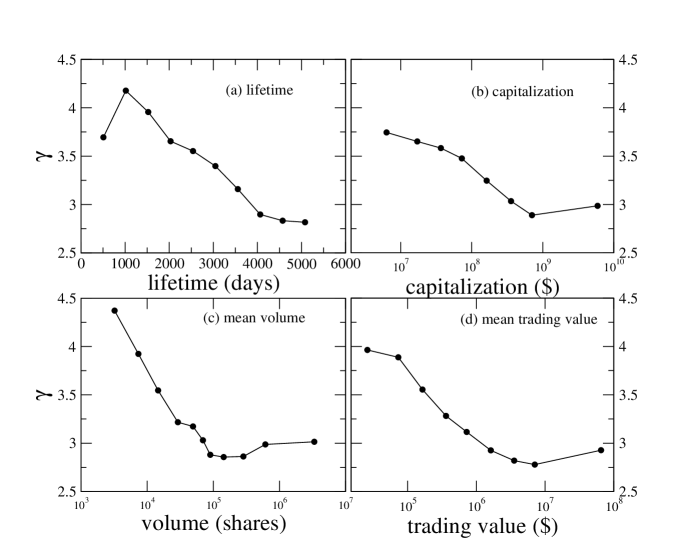
Figure 3: The power-law tail exponent $\gamma$ for different subsets of stocks. (a) Stocks are sorted into 10 subsets of different lifetime. Exponent $\gamma$ are abtained by fitting the PDF of volume volatility return intervals for each subset; (b) stocks are sorted into 8 subsets for different capitalization; (c) stocks are sorted into 11 subsets for different mean volume; (d) stocks are sorted into 9 subsets for different trading value.

In Figs. 2(b), 2(c), and 2(d), we show a similar tendencies for stock bins with different capitalizations, mean volumes, and mean trading values. Trading value is defined as stock price multiplied by transaction volume. For each stock, we designate the lifetime average of capitalization, volume, and trading value as performance indices. For example, the power-law exponents of the PDFs, $P_{q}(\tau)\langle\tau\rangle$, increase as the capitalization becomes larger [see Fig. 2(b)]. To clarify the picture, we divide all stocks into different subsets and study the behavior of the power-law exponent $\gamma$ with regard to these four factors. In Fig. 3(a), stocks are sorted into 10 subsets, from 508 days (2 years) to 5080 days (10 years). We fit the power-law tails of the volume return intervals for each subset and plot the exponent $\gamma$ versus the lifetime of the stocks. In Fig. 3(a), we can observe a systematic trend with stock lifetime. It is seen that a smaller exponent $\gamma$ which indicates a stronger correlation in older stock subsets. Similarly, we sort the stocks by capitalization, mean volume, and mean trading value, as shown in Figs. 3(b), 3(c), and 3(d). It is seen that $\gamma$ decreases with increasing of all these three factors but seem to become constant for large values of capitalizations, mean volumes and mean trading values.

Since all factors similarly affect the scaling of the PDF, $P_{q}(\tau)\langle\tau\rangle$, we now determine how much these factors are correlated. To study the relations between different stock bins, we plot the relation between trading value versus capitalization, mean volume versus capitalization, and mean trading value versus mean volume for all the stocks shown in Fig. 3. We see that larger capitalization stocks tend to have a larger trading volume and a larger trading value, which is consistent with Figs. 1(b), 1(c), and 1(d). The correlation coefficients between trading value and capitalization, mean volume and capitalization, and trading value and volume are 0.62, and 0.55, and 0.78, respectively. The correlation coefficients are high because these capitalization, volume, and trading value factors are all affected by firm size. Our analyses do not, however, show a significant relationship between stock lifetime and its trading value, capitalization, and mean volume, and the correlation coefficients are all $<0.20$.

V Short-term Memory Effects

We characterize a sequence of volume return intervals in terms of the autocorrelations in the time series. If the volume return intervals series are uncorrelated and independent of each other, their sequences can be determined only by the probability distribution. On the other hand, if the series is auto-correlated, the preceding value will have a memory effect on the values following in the sequence of volume volatility return intervals.

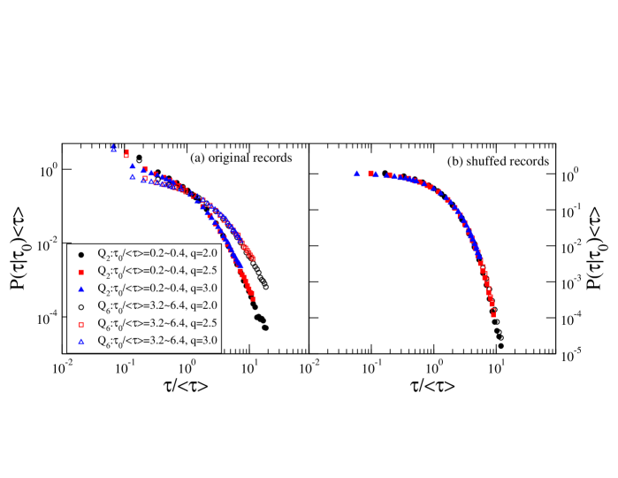
Figure 5: (Color online) Conditional PDF $P_{q}(\tau|\tau_{0})$ of volume volatility return intervals $\tau$ for different thresholds $q=2.0,2.5,3.0$, as a function of $\tau/\langle\tau\rangle$ for different $\tau_{0}/\langle\tau\rangle$ bins. A small $\tau_{0}$ subset $Q_{2}$ (full symbols) and a large $\tau_{0}$ subset $Q_{6}$ (open symbols) are displayed in (a). For example, subset $Q_{6}$ contains events of finding $\tau$ after large interval $3.2<\tau_{0}/\langle\tau\rangle<6.4$. In contrast to subset $Q_{6}$, subset $Q_{2}$ has larger probability to be followed by small $\tau/\langle\tau\rangle$ and smaller probability to be followed by large $\tau/\langle\tau\rangle$, which indicates short term correlation in the records: small intervals are followed by small intervals and large intervals are followed by large intervals. There is no memory effect in shuffle records as seen in (b) that the PDFs of all the subsets collapse onto one curve.

In order to investigate whether short-term memory is present, we study the conditional PDF, $P_{q}(\tau|\tau_{0})$, which is the probability of finding a volume return interval $\tau$ immediately after an interval of size $\tau_{0}$. In records without memory, $P_{q}(\tau|\tau_{0})$ should be identical to $P_{q}(\tau)$ and independent of $\tau_{0}$. Otherwise, $P_{q}(\tau|\tau_{0})$ should depend on $\tau_{0}$. Because the statistics for $\tau_{0}$ of a single stock are of poor quality, we study $P_{q}(\tau|\tau_{0})$ for a range of $\tau_{0}/\langle\tau\rangle$. The entire dataset is partitioned into eight equal-sized subsets, $Q_{1},Q_{2},...Q_{8}$, with intervals of increasing size $\tau_{0}/\tau$. Figure 5 shows the PDFs $P_{q}(\tau|\tau_{0})$ for $Q_{2}$, i.e., small interval size $0.2<\tau_{0}/\langle\tau\rangle<0.4$ and $Q_{6}$ large interval size $3.2<\tau_{0}/\langle\tau\rangle<6.4$ for different $q$. The probability of finding large $\tau/\langle\tau\rangle$ is larger in $Q_{6}$ (open symbols) than in $Q_{2}$ (full symbols), while the probability of finding small $\tau/\langle\tau\rangle$ is larger in $Q_{2}$ than that in $Q_{6}$. Thus large $\tau_{0}$ tends to be followed by large $\tau$, and vice versa, which indicates short-term memory in the volume return intervals sequence. Moreover, note that $P_{q}(\tau|\tau_{0})$ in the same subset for different thresholds $q$ fall onto a single curve, which indicates the existence of a unique scaling for the conditional PDFs as well. Similar results were found for the volume volatility of the Chinese markets Ren10 and for price volatilities Yamasaki05 ; Wang06 .

VI Long-term Memory Effects

In previous studies, the price volatility series was shown to have long-term correlations. Using a similar approach, we test whether the volume volatility sequence also possesses long-term correlations. To answer this question, we employ the detrended fluctuation analysis (DFA) method Peng94 ; Bunde00 ; Kantelhardt01 to further reveal memory effects in the volume volatility series. Using the DFA method, we divide an integrated time series into boxes of equal length $n$ and fit a least squares line in each box. Next we compute the root-mean-square fluctuation $F(n)$ of the detrended time series within a window of $n$ points and determine the correlation exponent $\alpha$ from the scaling function $F(n)\sim n^{\alpha}$, where $\alpha\in[0,1]$. The correlation exponent $\alpha$ characterizes the autocorrelation in the sequence. The time series has a long-term memory and a positive correlation if the exponent factor $\alpha>0.5$, indicating that large values tend to follow large values and small values tend to follow small values. The time series is uncorrelated if $\alpha=0.5$ and anti-correlated if $\alpha<0.5$.

Using the DFA method, we analyze the price volatility and volume volatility time series by plotting in bins the relation between correlation exponent $\alpha$ and the four financial factors, including stock lifetime, market capitalization, mean trading volume, and mean trading value. All the price volatility and volume volatility correlation exponents are significantly larger than 0.5, suggesting the presence of long-term memory in both price volatility sequences and volume volatility sequences. In all of the plots, the price volatility series shows a stronger long-term correlation than the volume volatility series. Moreover, as shown in Fig. 6(a), $\alpha$ on average increases for the stocks with a lifetime ranging from 350 days to 3800 days (about 15 years), and then shows a slight decrease, suggesting that long-lasting stocks tend to have a persistent price and volume movement on large scales. The increasing exponent $\alpha$ indicates that the volume volatility of older stocks is more correlated than that of younger stocks. This is consistent with the indication in Fig. 2(a) that the volume volatility of older stocks are more auto-correlated. Figures 6(b),  6(c), and  6(d) show that there is no systematic tendency relation between $\alpha$ and market capitalization, trading volume, and trading value.

VII conclusions

We have shown the scaling properties and memory effect of volume volatility return intervals in large stock records of the U.S. market. The scaled distribution of volume volatility return intervals displays unique power-law tails for different thresholds $q$. We also find different power-law exponents $\gamma$ of $P_{q}(\tau)$ for the four essential stock factors: stock lifetime, market capitalization, average trading volume, and average trading value. These different exponents may be related to long-term correlations in the interval series. Significantly, the daily volume volatility exhibits long-term correlations, similar to that found for price volatility. The conditional probability, $P_{q}(\tau|\tau_{0})$ for $\tau$ following a certain interval $\tau_{0}$, indicates that volume return intervals are short-term correlated.

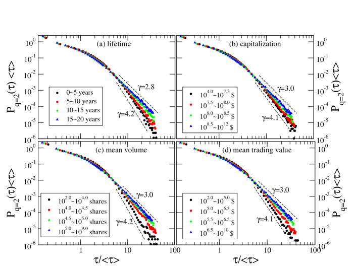
Figure 2: (Color online) Relations between distribution function $P_{2}(\tau)\langle\tau\rangle$ of volume volatility return intervals and four financial factors: (a) lifetime, (b) market capitalization, (c) average daily trading volume, (d) average daily trading value, for the threshold $q=2.0$. The distrition functions decay with various exponents $\gamma$ and show similar systematic tendency for four financial factors.

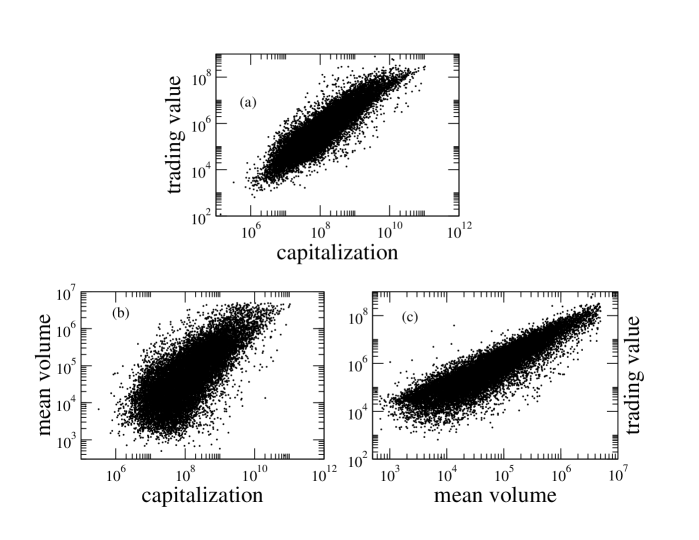
Figure 4: Scatter plots for the relations in stocks between trading value and capitalization, mean volume and capitalization, trading value and mean volume for all 17,197 stocks. For example, a point on panel (a) represents a stock, which has $ $10^{8}$ capitalization and $ $10^{6}$ average trading value. The correlation coefficients between trading value and capitalization, mean volume and capitalization, trading value and volume are 0.62, and 0.55, and 0.78 respectively.

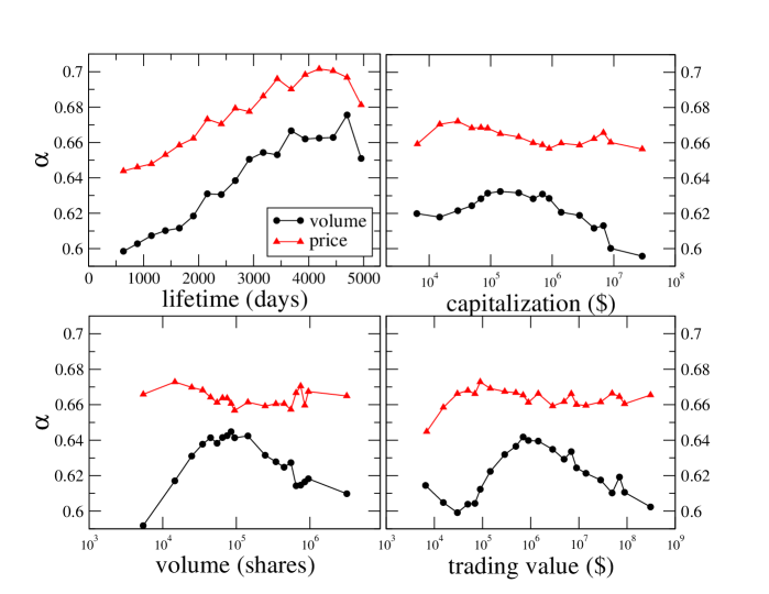
Figure 6: (Color online) Correlation exponent $\alpha$ obtained from detrended fluctuation analysis (DFA) of volume volatility (square) and price volatility (triangle). The plot shows the relation between $\alpha$ and four factors: (a) lifetime, (b) market capitalization, (c) average daily trading volume, (d) average daily trading value, for the threshold $q=2.0$.

References

- (1) B. B. Mandelbrot, J. Business 36, 394 (1963).
- (2) R. N. Mantegna and H. E. Stanley, Nature (London) 376, 46 (1995).
- (3) Econophysics: An Emerging Science, edited by I. Kondor and J. Kertész (Kluwer, Dordrecht, 1999).
- (4) R. Mantegna and H. E. Stanley, Introduction to Econophysics: Correlations and Complexity in Finance (Cambridge University Press, Cambridge, England, 2000).
- (5) H. Takayasu et al., Physica A 184, 127 (1992); H. Takayasu et al., Phys. Rev. Lett. 79, 966 (1997); H. Takayasu et al., Fractals 6, 67 (1998).
- (6) J.-P Bouchaud and M. Potters, Theory of Financial Risk: From Statistical Physics to Risk Management (Cambridge University Press, Cambridge, England, 2000).
- (7) N. F. Johnson, P. Jefferies, and P. M. Hui, Financial Market Complexity (Oxford University Press, New York, 2003).
- (8) Y. Liu, P. Gopikrishnan, P. Cizeau, M. Meyer, C.-K. Peng, and H. E. Stanley, Phys. Rev. E 60, 1390 (1999).
- (9) V. Plerou et al., Quant. Finance 1, 262 (2001); V. Plerou et al., Phys. Rev. E 71 , 046131 (2005).
- (10) Z. Ding, C. W. J. Granger, and R. F. Engle, J. Empirical Finance 1, 83 (1993).
- (11) R. A. Wood, T. H. McInish, and J. K. Ord, J. Financ. 40, 723 (1985).
- (12) L. Harris, J. Financ. Econ. 16, 99 (1986).
- (13) A. Admati and P. Pfleiderer, Rev. Financ. Stud. 1, 3 (1988).
- (14) G. W. Schwert, J. Financ. 44, 1115 (1989); K. Chan, K. C. Chan, and G. A. Karolyi, Rev. Financ. Stud. 4, 657 (1991); T. Bollerslev, R. Y. Chou, and K. F. Kroner, J. Econometr. 52, 5 (1992); A. R. Gallant, P. E. Rossi, and G. Tauchen, Rev. Financ. Stud. 5, 199 (1992); B. Le Baron, J. Business 65, 199 (1992).
- (15) M. M. Dacorogna, U. A. Muller, R. J. Nagler, R. B. Olsen, and O. V. Pictet, J. Int. Money Finance 12, 413 (1993).
- (16) A. Pagan, J. Empirical Finance 3, 15 (1996).
- (17) C. W. J. Granger and Z. Ding, J. Econometr. 73, 61 (1996).
- (18) Y. Liu, P. Cizeau, M. Meyer, C.-K. Peng, and H. E. Stanley, Physica A 245, 437 (1997).
- (19) R. Cont, Ph.D. thesis, Université de Paris XI, Orsay, 1998; see also R. Cont, e-print arXiv:cond-mat/9705075.
- (20) P. Cizeau, Y. Liu, M. Meyer, C.-K. Peng, and H. E. Stanley, Physica A 245, 441 (1997).
- (21) M. Pasquini and M. Serva, Econ. Lett. 65, 275 (1999).
- (22) K. Yamasaki, L. Muchnik, S. Havlin, A. Bunde, and H. E. Stanley, Proc. Natl. Acad. Sci. USA 102, 9424 (2005).
- (23) F. Wang, K. Yamasaki, S. Havlin, and H. E. Stanley, Phys. Rev. E 73, 026117 (2006).
- (24) F. Wang, P. Weber, K. Yamasaki, S. Havlin, and H. E. Stanley, Eur. Phys. J. B 55, 123 (2007).
- (25) A. Bunde, J. F. Eichner, S. Havlin, and J. W. Kantelhardt, Physica A 342, 308 (2004).
- (26) A. Bunde, J. F. Eichner, J. W. Kantelhardt, and S. Havlin, Phys. Rev. Lett. 94, 048701 (2005).
- (27) V. N. Livina, S. Havlin, and A. Bunde, Phys. Rev. Lett. 95, 208501 (2005).
- (28) S. Lennartz, V. N. Livina, A. Bunde and S. Havlin, Europhys. Lett. 81, 69001 (2008).
- (29) E. G. Altmann and H. Kantz, Phys. Rev. E 71, 056106 (2005).
- (30) T. Lux, Appl. Financ. Econ. 6, 463 (1996)
- (31) V. Plerou, P. Gopikrishnan, L. A. Nunes Amaral, X. Gabaix and H. E .Stanley, Phys. Rev. E 62, R3023 (2000).
- (32) P. Gopikrishnan, V. Plerou, X. Gabaix and H. E .Stanley, Phys. Rev. E 62, R4493 (2000).
- (33) V. Plerou and H. E. Stanley, Phys. Rev. E 76, 046109 (2007).
- (34) V. Plerou and H. E. Stanley, Phys. Rev. E 79, 068102 (2009).
- (35) F. Ren, W. Zhou, Phys. Rev. E 81, 066107 (2010).
- (36) W.-S. Jung, F. Wang, S. Havlin, T. Kaizoji, H.-T. Moon, and H. E. Stanley, Eur. Phys. J. B 62, 113 (2008).
- (37) M. I. Bogachev, J. F. Eichner, and A. Bunde, Phys. Rev. Lett. 99, 240601 (2007).
- (38) C.-K. Peng, S. V. Buldyrev, S. Havlin, M. Simons, H. E. Stanley, and A. L. Goldberger, Phys. Rev. E 49, 1685 (1994); C.-K. Peng, S. Havlin, H. E. Stanley, and A. L. Goldberger, Chaos 5, 82 (1995).
- (39) A. Bunde, S. Havlin, J. W. Kantelhardt, T. Penzel, J.-H. Peter, and K. Voigt, Phys. Rev. Lett. 85, 3736 (2000).
- (40) J. W. Kantelhardt, E. Koscielny-Bunde, H. A. Rego, S. Havlin, A. Bunde, Physica A 295, 441 (2004)