Lagrangian Descriptors: A Method for Revealing Phase Space Structures of General Time Dependent Dynamical Systems

Abstract

In this paper we develop new techniques for revealing geometrical structures in phase space that are valid for aperiodically time dependent dynamical systems, which we refer to as Lagrangian descriptors. These quantities are based on the integration, for a finite time, along trajectories of an intrinsic bounded, positive geometrical and/or physical property of the trajectory itself. We discuss a general methodology for constructing Lagrangian descriptors, and we discuss a “heuristic argument” that explains why this method is successful for revealing geometrical structures in the phase space of a dynamical system. We support this argument by explicit calculations on a benchmark problem having a hyperbolic fixed point with stable and unstable manifolds that are known analytically. Several other benchmark examples are considered that allow us the assess the performance of Lagrangian descriptors in revealing invariant tori and regions of shear. Throughout the paper “side-by-side” comparisons of the performance of Lagrangian descriptors with both finite time Lyapunov exponents (FTLEs) and finite time averages of certain components of the vector field (‘time averages”) are carried out and discussed. In all cases Lagrangian descriptors are shown to be both more accurate and computationally efficient than these methods. We also perform computations for an explicitly three dimensional, aperiodically time-dependent vector field and an aperiodically time dependent vector field defined as a data set. Comparisons with FTLEs and time averages for these examples are also carried out, with similar conclusions as for the benchmark examples.

Keywords: Invariant manifolds, nonautonomous systems, aperiodically time-dependent vector fields, transport barriers.

1 Introduction

Since the insights of Poincaré (1890) geometrical structures in phase space have played a central role in characterizing the global behaviours of dynamical systems. This point of view gives insight into the evolution of qualitatively distinct classes of trajectories without having to explicitly integrate and compare the behaviour of trajectories. This point of view has also been shown to provide much insight into fluid transport and mixing after the recognition that the equations for incompressible fluid particle motion (in the absence of molecular diffusion) are formally equivalent to Hamilton’s equations where, in the fluid mechanics context, the stream function plays the role of the Hamiltonian function and the physical space in which the fluid moves plays the role of the phase space of the corresponding Hamilton’s equations Aref (1984). This framework for studying fluid transport and mixing is often referred to as the ‘dynamical systems approach to Lagrangian transport” since the focus is on understanding the “organising structures” in phase space for fluid particle trajectories. References describing this approach for general fluid mechanics are Ottino (1989); Wiggins and Ottino (2004), and references specific to geophysical fluid dynamics are Jones and Winkler (2002); Wiggins (2005); Mancho et al. (2006c); Samelson and Wiggins (2006).

In this paper we further develop a technique for revealing phase space structure that was proposed and used in Mendoza and Mancho (2010); Mendoza et al. (2010); Mendoza and Mancho (2012); de la Cámara et al. (2012). This method is based on the computation of arc length of particle trajectories and it is extended by considering the integration of a bounded, positive quantity that is an intrinsic geometrical and/or physical property of the dynamical system along trajectories of the dynamical system, for a finite time. Techniques based on the integration of properties along trajectories have been used in the past. Rypina et al. (2011) have proposed methods based on the idea of complexity of isolated trajectories. Recently in the computer graphics community, Acar et al. (2012) have also used the time-normalized arc length of trajectories for human action recognition. Their work is inspired on the line integral convolution discussed by Shi et al. (2008); Cabral and Leedom (1993) that advect conserved physical fields along trajectories. The advection of conserved physical fields has been also used in the atmospheric science community since the early 90s. O’Neill et al. (1994); Sutton et al. (1994) proposed the reverse domain filling method for visualizing transport structures in geophysical flows. Recently in the context of realistic oceanic flows the works by Prants et al. (2011a, b) have highlighted Lagrangian features by computing the time of exit of particles from a given region or the number of changes of the sign of zonal and meridional velocities. Huhn et al. (2012) and Prants (2013) have addressed similar purposes by measuring the absolute displacements of particles and Prants et al. (2013) by counting the number of cyclonic and anticyclonic rotations of particles.

The techniques explained in the current article have been shown to be effective for revealing phase space structures for aperiodically time dependent flows. In Section 2 we describe the general methodology for constructing Lagrangian descriptors, and we emphasise the role of the norm in quantifying the integral of the chosen positive quantity along trajectories. Section 2.1 describes the performance of Lagrangian descriptors in hyperbolic regions, and Section 2.1.1 discusses the benchmark problem of a linear, autonomous vector field in the plane having a hyperbolic saddle point at the origin. This is an excellent example, not only for discussing the issues associate with the performance of Lagrangian descriptors, but also for comparing their performance with finite time Lyapunov exponents (FTLEs) and time averages of particular components of the vector field along trajectories since the stable and unstable manifolds of the hyperbolic point, as well as all trajectories, are known exactly. In this example we are able to illustrate the effect of the integration time and make precise the idea that “singular contours of the Lagrangian descriptors correspond to invariant manifolds”, both numerically, and analytically in Section 2.1.2. This example also illustrates why the $L^{\gamma}$ norms, $\gamma>1$ are not successful in revealing ”singular contours” in the same way as the $L^{\gamma}$ norms, $\gamma\leq 1$. In Section 2.3 we show that for this example FTLEs completely fail to reveal any phase space. Since the system is linear almost all FTLEs, for any time, are equal for every trajectory. A similar failure for finite time averages of a component of the vector field along trajectories is reported in Section 2.3.2. In Section 2.2 we consider another benchmark example –a linear vector field having an elliptic equilibrium point at the origin. As in the example of the linear saddle point, since this system is linear almost all FTLEs are zero, for any time. Hence the FTLE field fails to reveal any phase space structure. The Lagrangian descriptors, on the other hand, reveal the expected phase space structure, consistent with the trajectories. Since this example is linear elliptic point, effects of shear are not considered. In Section 2.2.2 we consider an integrable example in action-angle coordinates (hence all FTLEs are zero, for any time) that not only contain regions of strong shear, but also invariant tori where the “twist condition” breaks down (i.e. “twistless tori”). We show that Lagrangian descriptors provide signatures of each of these features. An advantage of the linear saddle point and linear elliptic point examples is that they allow us to “isolate” hyperbolic and elliptic behaviour. In Section 2.4 we consider the forced Duffing equation for three different types of time dependency: 1) no time dependency (forcing), i.e. the integrable case, 2) periodic time dependence, and 3) aperiodic time dependence (of a form that we define). In this example hyperbolic and elliptic behaviour are “intermingled” in a complicated manner (that we describe), and this affords us an ideal setting to compare Lagrangian descriptors, FTLEs, and averages of velocity components along trajectories “side-by-side” in different regions of the phase space of the forced Duffing oscillator. In Section 3 we consider a three dimensional vector field from fluid mechanics –the Hill’s spherical vortex subjected to a time-aperiodic perturbation-that was studied in Branicki and Wiggins (2009). For this example we show that Lagrangian descriptors provide an efficient way of discovering and visualising detailed geometrical structures in the flow. A comparison is made with FTLEs and averages of components of the vector field along trajectories, and it is shown that these techniques may introduce “artefacts” that obscure the true geometric structures. In Section 4 we consider velocity fields defined as data sets. In particular, we consider a wind driven three-layer quasigeostrophic simulation in a rectangular domain in a “double gyre” configuration exhibiting aperiodic time dependence. This velocity field has been the subject of earlier studies (Coulliette and Wiggins (2001); Mancho et al. (2004, 2006c)) and therefore allows us to directly compare the performance of Lagrangian descriptors and FTLEs with distinguished hyperbolic trajectories (DHTs) and their stable and unstable manifolds. Additionally, we compare the convergence time of Lagrangian descriptors with FTLEs to the stable and unstable subspaces of a given DHT, where we see that the Lagrangian descriptors converge to these structures more quickly. In Section 5 we compare the computational effort required for Lagrangian descriptor computations with FTLE computations, and in Section 6 we summarise our conclusions. In three appendices we provide some additional technical details.

2 Lagrangian Descriptors: Definitions, Heuristics, and Analytical Results

The concept of a Lagrangian descriptor was first introduced in Mendoza and Mancho (2010). There it was shown that this tool is able to provide a global dynamical picture of the geometric structures for arbitrary time dependent flows. In particular, Lagrangian descriptors are able to detect the main “organising centres” in the flow – hyperbolic trajectories and their stable and unstable manifolds and elliptic regions. In this section we describe precisely what we mean by the term “Lagrangian descriptor”. We then provide a heuristic justification for why they “work”. We build on this by then considering several benchmark examples where the phase space structure and stability characteristics are known analytically. This allows a deeper investigation of the heuristic justification, as well as a comparison with other commonly used method for extracting phase space structures, such as finite time Lyapunov exponents (FTLEs).

We consider a general time-dependent vector field on $\mathbb{R}^{n}$:

$$\frac{d{\bf x}}{dt} = {\bf v}({\bf x},t),\,\,{\bf x}\in\,\mathbb{R}^{n},\,t\in\,\mathbb{R}$$ (1)

where we assume that ${\bf v}({\bf x},t)$ is $C^{r}$ ($r\geq 1$) in ${\bf x}$ and continuous in $t$. This is a sufficient condition for the existence of unique solutions that also allows for linearization. The time interval on which a solution exists is also an issue. However, we will proceed by assuming that the solutions exist for a sufficient time so that the integral expressions we derive have validity, and then we will verify the validity in specific examples.

We begin by describing the Lagrangian descriptor first described in Mendoza and Mancho (2010). In that reference it was denoted by $M$, but henceforth we will denote it by $M_{1}$ since we will introduce additional Lagrangian descriptors. $M_{1}$ is the Euclidean arc length of the curve in phase space defined by a trajectory of (1) that starts at ${\bf x^{*}}$ at time $t=t^{*}$ for the time interval $[t^{*}-\tau,t^{*}+\tau]$, i.e.

$$M_{1}({\bf x^{*}},t^{*})_{{\bf v},\tau}=\int^{t^{*}+\tau}_{t^{*}-\tau}\!\!\!\sqrt{\sum_{i=1}^{n}\left(\frac{dx_{i}(t)}{dt}\right)^{2}}dt=\int^{t^{*}+\tau}_{t^{*}-\tau}\|{\bf v}({\bf x}(t),t)\|dt,$$ (2)

where $(x_{1}(t),x_{2}(t),...,x_{n}(t))$ denote the components of the trajectory ${\bf x}(t)$ in $\mathbb{R}^{n}$ . Clearly, $M_{1}$ depends on the initial point $\bf x^{*}$ and the time interval $[t^{*}-\tau,t^{*}+\tau]$ (and the vector field $\bf v$).

A Heuristic Argument.

At this point it is insightful to give a heuristic argument as to why $M_{1}$ is useful for revealing the geometric structures in the phase space of (1). $M_{1}$ measures the arc-length of trajectories on a time interval $(t^{*}-\tau,t^{*}+\tau)$. Trajectories with “close” initial conditions that remain “close” as they evolve on the time interval $(t^{*}-\tau,t^{*}+\tau)$ are expected to have arc-lengths that are “close”. However, at the boundaries between regions comprising trajectories with qualitatively different behaviour in the course of their time evolution over the time interval $(t^{*}-\tau,t^{*}+\tau)$, we expect the arc-lengths of trajectories starting on either side of the boundary to not be “close” on the time interval. (Of course, this will depend on $\tau$, and the dependence on $\tau$ is an issue that we will shortly address.) Hence, these boundaries are denoted by an “abrupt change” in $M_{1}$, where “abrupt change” means that the derivative of $M_{1}$ transverse to these boundaries is discontinuous on the boundaries. This will be more precisely discussed and defined in Section 2.1. Such boundaries correspond to the stable and unstable manifolds of hyperbolic trajectories, if we are in a hyperbolic region, of the phase space. Hence, in this way $M_{1}$ detects stable and unstable manifolds of hyperbolic trajectories.

A General Construction for Lagrangian Descriptors.

The arc length of a segment of a trajectory, defined by (2), is obtained by integrating the modulus of the velocity ($\|{\bf v}\|$) along a trajectory for a time that parametrizes the curve. However, consistent with the heuristic argument given above, it is reasonable to expect this methodology to be successful for other positive scalar valued functions that embody an intrinsic physical or geometrical property of trajectories that are integrated along trajectories over the time interval $(t^{*}-\tau,t^{*}+\tau)$. For example, integration along trajectories of other positive scalar valued quantities could have been considered, such as the modulus of acceleration ($\|{\bf a}\|$), the modulus of the time derivative of acceleration ($\|d{\bf a}/dt\|$), or the modulus of combinations of ${\bf v}$, ${\bf a}$ or $d{\bf a}/dt$, with the only restriction being that the integrals of these quantities along trajectories are well-defined. The heuristic argument would still apply and indicate that at the boundaries of regions comprising trajectories with qualitatively different time evolutions the accumulated value of the chosen positive quantity will “change abruptly” in the sense that the derivative transverse to the boundary of the corresponding Lagrangian descriptor will be discontinuous on the boundary, and examples of such regions would be those that are separated by the stable and unstable manifolds of hyperbolic trajectories. For this reason abrupt changes in a Lagrangian descriptor, which are manifested as discontinuities on the boundary of the derivative of the Lagrangian descriptor transverse to the boundary, are seen as singular curves in contour plots of the Lagrangian descriptor, and these are expected to be related to invariant manifolds. We will see specific examples that make these ideas precise in the remainder of this section.

However, for now we note that based on this general reasoning a method for constructing families of Lagrangian descriptors for general time dependent flows would be as follows. Let $|\mathcal{F}({\bf x})|$ denote the bounded, positive intrinsic physical or geometrical property of the velocity field that is of interest. Consider a trajectory ${\bf x}(t)$ satisfying ${\bf x}(t^{*})={\bf x}^{*}$ and defined on the time interval $(t^{*}-\tau,t^{*}+\tau)$ (where $\tau$ is “appropriately chosen”, as we will shortly discuss). Then $|\mathcal{F}({\bf x}(t))|$ is a scalar valued function of $t$ that depends parametrically on ${\bf x}^{*}$ and $t^{*}$. Therefore for $\gamma\leq 1$ we can consider its $L^{\gamma}$ norm:

$$M({\bf x^{*}},t^{*})_{{\bf v},\tau}=\left(\int^{t^{*}+\tau}_{t^{*}-\tau}|\mathcal{F}({\bf x}(t))|^{\gamma}\,dt\right).$$ (3)

Alternatively for $\gamma>1$ the $L^{\gamma}$ norm is given by:

$$M({\bf x^{*}},t^{*})_{{\bf v},\tau}=\left(\int^{t^{*}+\tau}_{t^{*}-\tau}|\mathcal{F}({\bf x}(t))|^{\gamma}\,dt\right)^{\frac{1}{\gamma}}.$$ (4)

For example, for (2) we considered the $L^{1}$ norm of the magnitude of the velocity evaluated on trajectories defined on the time interval $(t^{*}-\tau,t^{*}+\tau)$. Other choices are possible. For example, we could consider the $L^{\gamma}$ norm of the magnitude of the acceleration. For this case, for $\gamma=1$, we denote the resulting $M$ function by $M_{2}({\bf x^{*}},t^{*})_{{\bf v},\tau}$. We could also consider the $L^{\gamma}$ norm of the magnitude of the velocity or the acceleration. In this case we denote the resulting $M$ function by $M_{3}({\bf x^{*}},t^{*})_{{\bf v},\tau}$, and we will consider $M_{3}$ for both $\gamma=2$ and $\gamma=\frac{1}{2}$. Another possibility is to consider the $L^{1}$ norm of the magnitude of the time derivative of the acceleration, and in this case we denote the $M$ function by $M_{4}({\bf x^{*}},t^{*})_{{\bf v},\tau}$. We will explore more deeply the advantages and disadvantages of these different choices in the remainder of this section. However, we remark that the $L^{\gamma}$ norms, $\gamma>1$, are not useful as Lagrangian descriptors in the sense that they do not reveal significant underlying structures in the flow. We will explore the reasons for this in Section 2.1.1.

Finally, the curvature is an intrinsic property of curves. It is a positive quantity that combines both velocity and acceleration (Kreyszig (1991)):

$$\kappa=\frac{\sqrt{({\bf v}\cdot{\bf v})({\bf a}\cdot{\bf a})-({\bf v}\cdot{\bf a})^{2}}}{({\bf v}\cdot{\bf v})^{3/2}}$$ (5)

The value of the curvature ranges from zero to infinity–the curvature of straight lines is zero and the curvature of fixed points is infinity. We define a Lagrangian descriptor based on curvature as follows:

$$|\mathcal{F}_{5}({\bf x}(t))|=\frac{1}{|\kappa({\bf x}(t))|+a}$$ (6)

where singularities are avoided by introducing $a>0$ in the denominator. We have numerically verified that good choices for ‘$a$’ lie in the interval $5>a>1$. This interval is determined considering that if ‘$a$’ is very large then Eq. (6) tends to be independent of $\kappa({\bf x}(t))$. On the other hand if ‘$a$’ is very small the expression (6) will present very sharp profiles for zero curvatures near straight lines. In the examples to follow we will present results for $a=1$.

A key property of all of the Lagrangian descriptors is that they are quantities that “accumulate” along a trajectory, i.e. they are integrals of a positive quantity along a trajectory. The heuristic argument would not be valid for the integral of a quantity that changes sign along a trajectory. We will address this issue explicitly in Section 2.3. In Table 1 we summarize the different Lagrangian descriptors that we have introduced in this section

Lagrangian Descriptor	Integrand	Norm
$M_{1}$	magnitude of velocity	$L^{1}$
$M_{2}$	magnitude of acceleration	$L^{1}$
$M_{3}$	magnitude of acceleration or velocity	$L^{\frac{1}{2}}$ or $L^{2}$
$M_{4}$	magnitude of the time derivative of the acceleration	$L^{1}$
$M_{5}$	positive quantity related to curvature ( Eq. (6))	$L^{1}$

Table 1: The left hand column denotes the Lagrangian descriptors used, the middle column describes the positive quantities used as the integrand for the Lagrangian descriptors, the right hand column describes the norm that is used.

and Appendix A describes in detail issues associated with the numerical computation of Lagrangian descriptors.

Hyperbolic and Elliptic Regions.

The phrases “hyperbolic regions” and “elliptic regions” occur throughout the literature. Here we want to consider their meaning more carefully.

Traditionally, the words “elliptic” and “hyperbolic” have referred to the stability characteristics of individual trajectories. Trajectories are said to be hyperbolic if none of its Lyapunov exponents are zero (with the exception of the Lyapunov exponent tangent to the direction of motion of the trajectory, i.e. the Lyapunov exponent in the direction of the velocity). Exponential dichotomies are also, equivalently, used to characterise hyperbolicity, see Coppel (1978); Dieci et al. (1997); Dieci and Vleck (2002). These characterisations of hyperbolicity are independent of the nature of the time dependence. The definition of “elliptic” for general time dependent trajectories has not received the same level of attention, at least in the applied areas. Certainly, the notion of “elliptic stability type” for time periodic trajectories is well established. A time periodic trajectory is elliptic if all of its Floquet multipliers lie on the unit circle (there are some issues when a multiplier is $1$ or $-1$, but that level of technicality is not important for our discussion).

However, there is a significant body of literature that does address the notion of “elliptic stability” for trajectories in vector fields having arbitrary (e.g. aperiodic) time dependence. It would be very interesting to explore the implications of these ideas in applications, in much the same way that Lyapunov exponents have been explored and exploited in applications. However, here we are considering what is meant by the phrases “hyperbolic region” and “elliptic region”.

With the notion of hyperbolic and elliptic stability of individual trajectories in hand, we can now address the question of what is meant by the phrases “hyperbolic region” and “elliptic region”. Initially, one might guess that these are regions (e.g. open sets) having the property that all trajectories in such regions are either elliptic or hyperbolic. However, there is an issue with this particular definition that requires careful consideration. Namely, traditionally notions of “elliptic” or “hyperbolic” stability type are infinite time characterisations of trajectories. Hence, in order to establish that all the trajectories in a region are of a particular stability type, one would need the trajectories to remain in that region for all time. In other words, one would need the region to be invariant (at least in forward time). This requirement could (naturally) be met for linear or integrable Hamiltonian systems, but not for general dynamical systems. There is an additional complication that occurs for “generic” dynamical systems (at least for dynamical systems defined by time periodic velocity fields). General theoretical results imply that it is unreasonable to assume that we can “cleanly” separate dynamical behaviour into “hyperbolic” and “elliptic”. In particular, conservative generalisations of the “Newhouse phenomena” Newhouse (1977); Duarte (1999); Gonchenko and Silnikov (2000) imply that tangencies between the stable and unstable manifolds of hyperbolic trajectories are “persistent” and will give rise to elliptic “islands of stability”. If one “perturbs away” such tangencies, then new ones will be created elsewhere. We emphasis that, to date, such results have only been proven in the time-periodic setting.

Despite ambiguities, it has nevertheless proved useful in the fluid mechanical situation to attempt to partition the flow into “elliptic” and “hyperbolic” regions. Early attempts in the fluids community to achieve such a decomposition of the flow led to the Okubo-Weiss criterion (Okubo (1970); Weiss (1991)), which is essentially Eulerian in nature. Efforts to generalize the idea to a Lagrangian setting appeared in Haller (2001) (but see also Duc and Siegmund (2008); Branicki and Wiggins (2010)). This is not a problem that we will explicitly address in this paper. Nevertheless, we will use the phrases “hyperbolic region” and “elliptic region”, but for most usages we will be considering linear and integrable systems, where the difficulties mentioned above are not an issue.

2.1 Lagrangian Descriptors in Hyperbolic Regions

Hyperbolic regions contain the “seeds” of change, uncertainty, and chaos in flows. In particular, they contain hyperbolic trajectories and their stable and unstable manifolds. In this section we will explore the performance of the Lagrangian descriptors defined in the previous section in familiar examples that exhibit hyperbolic behaviour. We will also relate their performance to more familiar diagnostics for “diagnosing” phase space structure, such as finite time Lyapunov exponents (FTLEs) and the ergodic decomposition.

2.1.1 The Linear Saddle Point

The first example that we analyze is the linear saddle. Initially, one might consider this example as “too trivial”. However, we will show that it yields some interesting insights. Moreover, it lends itself to either exact, or accurate approximate, solutions for several interesting quantities in Section 2.3.

The velocity field that we consider is given by:

$$\dot{x} = \lambda x,$$

$$\dot{y} = -\lambda y,\quad\lambda>0,$$ (7)

and the flow generated by this velocity field is given by:

$$x(t,x_{0}) = x_{0}e^{\lambda t},$$

$$y(t,y_{0}) = y_{0}e^{-\lambda t},\quad\lambda>0,$$ (8)

The origin, $(x,y)=(0,0)$ is a hyperbolic fixed point with stable and unstable manifolds given by:

$$W^{s}\left(0,0\right) = \{(x,y)\in\mathbb{R}^{2}|x=0,\,y\neq 0\},$$ (9)

$$W^{u}\left(0,0\right) = \{(x,y)\in\mathbb{R}^{2}|y=0,\,x\neq 0\}.$$ (10)

In Figure 1 we show the evolution of the contours of $M_{1}$ for $\tau=0.5,2,\,10$. The first thing to observe is that the patterns of the contours displayed depend on $\tau$. For $\tau$ small the structure of $M_{1}$ is smooth and for increasing $\tau$ the contour patterns converge towards a structure that displays the manifolds by means of discontinuity in the derivatives. An analytical argument concerning the convergence time is given in Section 2.1.2.

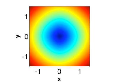
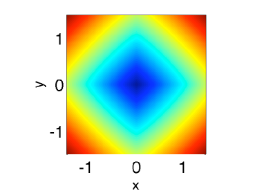
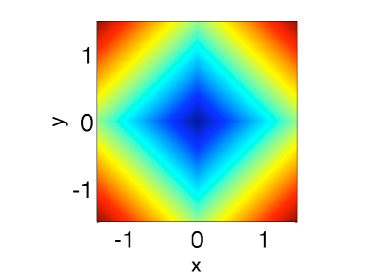
a) b) c) d)

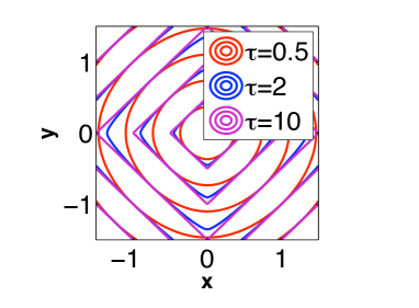
Figure 1: Evolution of the contours as $\tau$ increases. a) $\tau=0.5$, b) $\tau=2$, c) $\tau=10$, d) isolated contours showing the evolution for $\tau=0.5,\,2,\,10$.

In Figure 2 we show several different Lagrangian descriptors, where each is computed for $\tau=10$. Figure 2a) shows contours of the Lagrangian descriptor $M_{1}$ for $\lambda=1$. We see that the stable and unstable manifolds of the hyperbolic fixed point at the origin are easily identified. For $\lambda=1$ it is easy to see from the simple form of the velocity field (7) and its flow given in (8) that $M_{1}=M_{2}=M_{4}$, and therefore the latter two Lagrangian descriptors are not shown.

Figure 2b) shows the contours of $M_{3}$ for $\gamma=0.5$–the $L^{\frac{1}{2}}$ norm of the modulus of the acceleration–for which the stable and unstable manifolds of the hyperbolic fixed point at the origin are readily apparent. However, figure 2c) shows the contours of $M_{3}$ for $\gamma=2$–the $L^{2}$ norm of the modulus of the acceleration, and in this case the invariant manifolds structure is completely lost. We explain this behaviour in Section 2.1.2. In Figure 2d) we show contours of the Lagrangian descriptor $M_{5}$ (for $a=1$). In this case the manifolds are clearly shown. This is not surprising since the stable and unstable manifolds of the origin are the only trajectories having zero curvature. In fact, in this case we would expect that the contours of $M_{5}$ would reveal the manifolds for relatively small $\tau$. In particular, we have verified numerically that essentially the same contours are obtained for $\tau=2$.

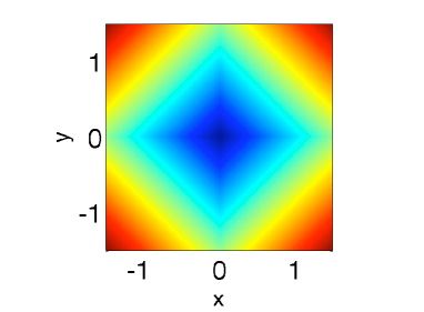
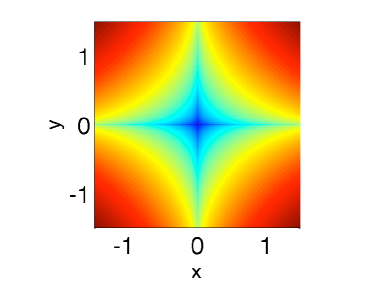
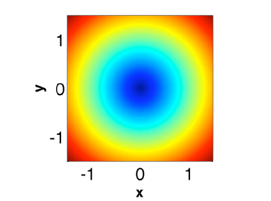
a) b) c) d)

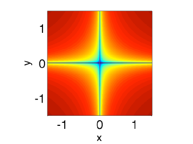
Figure 2: Contour plots for a selection of Lagrangian descriptors for (7). a) $M_{1}$; b) $M_{3}$, using the $L^{\frac{1}{2}}$ norm; c) $M_{3}$ using the $L^{2}$ norm; d) $M_{5}$.

Finally, we note that the Lyapunov exponents can be computed analytically for every trajectory in this example. Since the system is linear they are the same for every trajectory–$\pm\lambda$ (except for the exception case of trajectories starting on either the stable or unstable manifold of the origin, in which case one of the Lyapunov exponents will be zero). Hence the contours of constant Lyapunov exponents reveal no structure in this case (as noted in Branicki and Wiggins (2010)). This will be explored in more detail in Section 2.3.

2.1.2 Analytical Justification

In this section, for the specific example (7), we give analytical justification underlying the heuristic argument as to why contours of the Lagrangian descriptors having the property that the derivative of the Lagrangian descriptor transverse to the contours correspond to material curves. This also provides insight as to why the $L^{\gamma}$ norms, $\gamma>1$, do not reveal this singular property in the contours for Lagrangian descriptors that use such norms.

For (7), using (2), the $M_{1}$ function is given by:

$$M_{1}(x_{0},y_{0};t_{0},\tau)=\int_{t_{0}-\tau}^{t_{0}+\tau}\sqrt{\dot{x}(t,x_{0})^{2}+\dot{y}(t,y_{0})^{2}}dt=\int_{t_{0}-\tau}^{t_{0}+\tau}\sqrt{x_{0}^{2}\lambda^{2}e^{2\lambda t}+y_{0}^{2}\lambda^{2}e^{-2\lambda t}}dt$$ (11)

This function is clearly nonnegative since it is a measure of arc length of a trajectory. It is clear by inspecting (2) that $M_{1}(0,0;t_{0},\tau)=0$. This makes sense since the arc length of a point is zero. We want to compute the integral $M_{1}$. For simplicity we assume without loss of generality that $t_{0}=0$ (this is always possible for an autonomous system after a time shift $t^{\prime}=t-t_{0}$ and by redefining the initial conditions $x_{0}$ and $y_{0}$).

As already noted the patterns of the contours displayed in Figure 1 depend on $\tau$. For $\tau$ small the contours are smooth but for increasing $\tau$ they develop singular features along the unstable and stable manifolds. The nature of what we mean by the phrase “singular features” will be explained in the following where we provide analytical justification that underlies this behaviour.

Behavior for Small $\tau$.

We now want to argue that for $\tau$ small, (11) does not display “sharp features” that are related to the stable and unstable manifolds of the hyperbolic fixed point of (7). Towards this end, we consider an expansion of the expression (11) for fixed $y_{0}$ that is valid for $x_{0}$ small (i.e. near the stable manifold) and for small $\tau$. The expansion has the following form:

$$M_{1}(x_{0},y_{0};t_{0},\tau) = \int_{-\tau}^{\tau}\sqrt{(x_{0}\lambda)^{2}e^{2\lambda t}+(y_{0}\lambda)^{2}e^{-2\lambda t}}dt$$ (12)

$$= \int_{-\tau}^{\tau}\left(e^{-\lambda t}\lambda|y_{0}|+\frac{e^{3\lambda t}\lambda|y_{0}|}{2y_{0}^{2}}x_{0}^{2}\right)dt+O(x_{0}^{4}).$$

It is important to notice that in the integrand $x_{0}$ is always multiplied by $e^{2\lambda t}$, thus if we want the “error terms” in the series expansion around $x_{0}=0$ to be small, then $e^{2\lambda t}$ should not be large, which means that $\tau$ should not be large, as we are assuming. The leading order terms in (12) can be explicitly computed, and are found to be:

$$M_{1,{\rm lo}}(x_{0},y_{0};t_{0},\tau) = \int_{-\tau}^{\tau}\left(e^{-\lambda t}\lambda|y_{0}|+\frac{e^{3\lambda t}\lambda|y_{0}|}{2y_{0}^{2}}x_{0}^{2}\right)dt,$$ (13)

$$= {\left(e^{\lambda\tau}-e^{-\lambda\tau}\right)}|y_{0}|+\frac{\left(e^{3\lambda\tau}-e^{-3\lambda\tau}\right)|y_{0}|}{6y_{0}^{2}}x_{0}^{2}.$$

For $y_{0}$ fixed, (13) is a smooth function of $x_{0}$. Figure 3 shows a comparison of the accuracy of (12) with (13) for $\tau=2$ along a horizontal line perpendicular to the stable manifold. More precisely, we fix $y_{0}=0.5$ and plot (12) (computed numerically, and shown with a solid line) and (13) (shown with a dashed line). It is clear from the figure that leading order terms (13) accurately approximate (12) in the interval $x_{0}\in[-0.01,0.01]$.

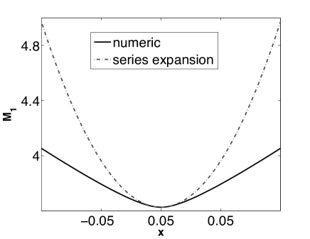
Figure 3: Solid line, the numerical evaluation of $M_{1}$ along $x_{0}$ for $y_{0}=0.5$, $\tau=2$, $\lambda=1$. Dashed line, the evaluation of the leading order terms (13).

Behavior for Large $\tau$.

Now we consider the behaviour of (11) when $\tau$ is large. Towards this end, we re-write (11) as follows:

$$M_{1}(x_{0},y_{0};t_{0},\tau)=\int_{0}^{\tau}\sqrt{X_{0}^{2}+Y_{0}^{2}}dt+\int_{-\tau}^{0}\sqrt{X_{0}^{2}+Y_{0}^{2}}dt$$ (14)

where we have defined $X_{0}^{2}=x_{0}^{2}\lambda^{2}e^{2\lambda t}$ and $Y_{0}^{2}=y_{0}^{2}\lambda^{2}e^{-2\lambda t}$.

In the first integral term in (14), since $t$ is positive if $\tau$ is large $X_{0}$ may assume large values for $t$ values approaching the upper limit of the integral. By similar reasoning, $Y_{0}$ will become small for $t$ values approaching the upper limit of integration. For the second integral term in (14), since the integration range is negative $Y_{0}$ assumes large values for $t$ approaching the lower limit of the integral. By similar reasoning, $X_{0}$ will become small for $t$ values approaching the lower limit of integration. These facts suggest isolating the large parts of both integral terms by choosing constants $\tau_{p},\,\tau_{n}>0$ (as we will see, precise values for these constants are not important for the argument) and re-writing (14) as follows:

$$M_{1}(x_{0},y_{0};t_{0},\tau) = \int_{\tau_{p}}^{\tau}\sqrt{X_{0}^{2}+Y_{0}^{2}}dt+\int_{0}^{\tau_{p}}\sqrt{X_{0}^{2}+Y_{0}^{2}}dt$$ (15)

$$+ \int_{-\tau_{n}}^{0}\sqrt{X_{0}^{2}+Y_{0}^{2}}dt+\int_{-\tau}^{-\tau_{n}}\sqrt{X_{0}^{2}+Y_{0}^{2}}dt$$

We expand the first term in (15) in $\frac{X_{0}}{Y_{0}}$ and the second term in (15) in $\frac{Y_{0}}{X_{0}}$ and rearrange the terms to obtain the following:

$$M_{1}(x_{0},y_{0};t_{0},\tau)=\int_{\tau_{p}}^{\tau}|X_{0}|dt+\int_{-\tau}^{-\tau_{n}}|Y_{0}|dt+O(1/X_{0})+O(1/Y_{0})+B,$$ (16)

where $B$ is defined as:

$$B=\int_{0}^{\tau_{p}}\sqrt{X_{0}^{2}+Y_{0}^{2}}dt+\int_{-\tau_{n}}^{0}\sqrt{X_{0}^{2}+Y_{0}^{2}}dt.$$ (17)

Using the fact that for $\tau$ large $|x_{0}|e^{\lambda\tau}>>|x_{0}|e^{\lambda\tau_{p}}$ and $|y_{0}|e^{\lambda\tau}>>|y_{0}|e^{\lambda\tau_{n}}$ it is straightforward to determine that the leading order terms of (16) are given by:

$$M_{1,{\rm lo}}(x_{0},y_{0};t_{0},\tau)=|x_{0}|e^{\lambda\tau}+|y_{0}|e^{\lambda\tau}.$$ (18)

In the above expressions it is important to note that the estimates are valid even if $x_{0}$ or $y_{0}$ are small as far as the products $x_{0}e^{\lambda t}$, $y_{0}e^{-\lambda t}$ are large. This occurs very close to the origin, $x_{0}\approx 0$ or $y_{0}\approx 0$, if $\tau$ is large, and this corresponds to a large integration time in the definition of the Lagrangian descriptor. In this case discontinuities in the derivatives (or even on the functions themselves in other possible examples) observed along the stable and unstable manifolds rise because the asymptotic expansions at both sides of the manifolds, do not match well across these lines. In practice for any finite $\tau$ the series expansion (12) is still valid, thus strictly speaking the function $M$ is regular, but it is accurate only in an extremely narrow gap around $x_{0}=0$, exponentially decreasing for increasing $\tau$.

Figure 4 shows a comparison of the accuracy of (14) with (18) for $\tau=10$ along a horizontal line perpendicular to the stable manifold. More precisely, we fix $y_{0}=0.5$, $\tau=10$, $\lambda=1$ and plot (14) (computed numerically, and shown in black) and (18) (shown in gray). It is clear from the figure that leading order terms (18) accurately approximate (14) in the interval $x_{0}\in[-0.1,0.1]$ and that the derivative of both functions appears discontinuous on the stable manifold.

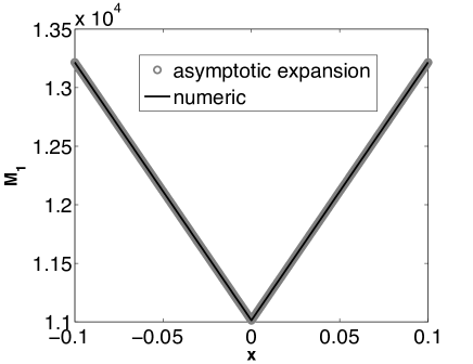
Figure 4: In black the numerical evaluation of (14) along $x_{0}$ for $y_{0}=0.5$, $\tau=10$, $\lambda=1$. In gray the evaluation of expression (18).

The $L^{\gamma}$ norm, $\gamma>1$.

In Section 2 we stated that the contours of the $L^{\gamma}$ norm, $\gamma>1$, of a bounded, positive intrinsic physical or geometrical property of the velocity field integrated along trajectories do not yield interesting structures in the flow. Here we give an argument why this is the case in the context of the example (7).

We first extend the previous results for the $L^{\gamma}$ norm, with $\gamma\leq 1$. The essential feature to consider is the exponent on the integrand, which we will take as the magnitude of velocity for this example:

$$M(x_{0},y_{0};t_{0},\tau)=\int_{-\tau}^{\tau}\left(X_{0}^{2}+Y_{0}^{2}\right)^{\delta}dt.$$ (19)

Following the same argument as above, in this case the asymptotic expansion is:

$$M(x_{0},y_{0};t_{0},\tau) \sim \int_{\tau_{p}}^{\tau}\left(X_{0}^{2\delta}+\delta Y_{0}X_{0}^{2(-1+\delta)}\right)dt+\int_{-\tau}^{-\tau_{n}}\left(Y_{0}^{2\delta}+\delta X_{0}Y_{0}^{2(-1+\delta)}\right)dt$$ (20)

$$+ O(1/X_{0}^{4-2\delta})+O(1/Y_{0}^{4-2\delta})$$

Following an argument similar to that given above, for $0<\delta<1$ the leading order terms in the expansion are:

$$M(x_{0},y_{0};t_{0},\tau)\sim\frac{|x_{0}|^{\gamma}}{\gamma}e^{\gamma\lambda\tau}+\frac{|y_{0}|^{\gamma}}{\gamma}e^{\gamma\lambda\tau}$$ (21)

where $\gamma=2\delta$. If $\gamma<1$ the derivative across the stable manifold is singular, which explains the enhancement of the features displayed in Figure 2b) for this choice of exponent. The case $\gamma=1$ corresponds to (2). On the other hand, if $\gamma>1$ the expression above should be raised to the power $1/\gamma$. In this case the derivative across the stable manifold is continuous. We see this in Figure 2c) ($\gamma=2$) for which the contours of $M$ are smooth.

2.2 Lagrangian Descriptors in Elliptic Regions

Now we will consider the behaviour of Lagrangian descriptors in “elliptic regions”. In the same spirit as in the discussion in Section 2.1.1, we will begin by discussing the familiar linear elliptic fixed point.

2.2.1 The Linear Elliptic Point

We consider the velocity field:

$$\dot{x} = y,$$

$$\dot{y} = -x,$$ (22)

and the flow generated by this velocity field is given by:

$$x(t,x_{0}) = x_{0}\cos t+y_{0}\sin t,$$

$$y(t,y_{0}) = -x_{0}\sin t+y_{0}\cos t.$$ (23)

The origin, $(x,y)=(0,0)$ is an elliptic fixed point. In this case the $M_{1}$ function has the form:

$$M_{1}(x_{0},y_{0};t_{0},\tau) = \int_{t_{0}-\tau}^{t_{0}+\tau}\sqrt{\dot{x}(t,x_{0})^{2}+\dot{y}(t,y_{0})^{2}}dt$$ (24)

$$= \int_{t_{0}-\tau}^{t_{0}+\tau}\sqrt{(-x_{0}\sin t+y_{0}\cos t)^{2}+(-x_{0}\cos t-y_{0}\sin t)^{2}}\,\,dt,$$

which is easily computed to give:

$$M_{1}(x_{0},y_{0};t_{0},\tau)=\int_{t_{0}-\tau}^{t_{0}+\tau}\sqrt{x_{0}^{2}+y_{0}^{2}}dt=2\tau\sqrt{x_{0}^{2}+y_{0}^{2}}.$$ (25)

which is a smooth function for all $\tau$ except at the origin. The contours of $M_{1}$, for any fixed $\tau$, are smooth circles surrounding the origin. Also, note that for this example it is easily verified that $M_{1}=M_{2}$.

2.2.2 An Integrable Example: Shear and Resonance

In this section we consider an example that, in some sense, is the “simplest” nonlinear problem that has entirely elliptic behaviour–a one degree-of-freedom integrable Hamiltonian system in action–angle variables. Nevertheless, this system provides some useful insights that raises questions for more complex systems.

The Hamiltonian is given by:

$$H(I)=\frac{I^{4}}{4}-\frac{I^{2}}{2},$$ (26)

and the associated Hamiltonian vector field is given by:

$$\dot{\theta}=\frac{\partial H}{\partial I} = I^{3}-I,$$

$$\dot{I}=-\frac{\partial H}{\partial\theta} = 0.\qquad\qquad(I,\theta)\in\mathbb{R}\times S^{1},$$ (27)

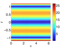
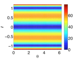
a) b) c)

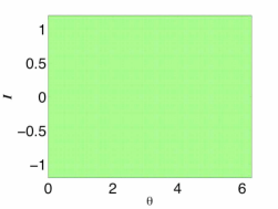
Figure 5: Evaluation of Lagrangian Descriptors for the system (27). a) $M_{1}$ for $\tau=25$; b)$M_{1}$ for $\tau=75$ ;c) $M_{3}$, using $||{\bf a}||$ in the integrand with the $L^{\frac{1}{2}}$ norm.

It is evident from (27) that $I$ is constant, and each value of $I$ corresponds to an invariant circle, or “invariant one torus” (since $\theta$ is periodic). The frequency of each torus is given by $\frac{\partial H}{\partial I}=I^{3}-I$ and the shear, or “twist” associated with each torus is $\frac{\partial^{2}H}{\partial I^{2}}=3I^{2}-1$. The typical behaviour for each $I=$ constant invariant circle is that it has nonzero frequency and nonzero shear. However, there are five exceptional tori that we note.

Resonance.

The three invariant circles $I=0$, $I=\pm 1$ correspond to circles of fixed points since the frequency is identically zero on each of these circles.

Zero shear.

On the invariant circles $I=\pm\frac{1}{\sqrt{3}}$ the frequencies are $\mp\frac{2}{3\sqrt{3}}$ but the shear, or “twist” is identically zero on each of these invariant circles. In the dynamical systems literature these are referred to as “twistless” invariant circles. The choice of “twist less” tori will allow us to compare with recent work in Beron-Vera et al. (2010) when we consider FTLEs in Section 2.3.

Figure 5a) illustrates how $M_{1}$ detects the three circles of fixed points (dark blue) as well as the high shear “twistless tori” (the reddish colours), for $\tau=25$. Figure 5b) shows the contours of $M$ for $\tau=75$, which contain essentially the same information as for $\tau=25$.

The function $M_{3}$, based on $||{\bf a}||$ and the $L^{\frac{1}{2}}$, gives a different perspective on the structure of the flow. Since in this system all trajectories move with constant velocity, their acceleration is zero, from which it follows that $M_{3}$ is identically zero. In this case Figure 5c) confirms a flat structure which is obtained for all $\tau>0$. That is, there is no convergence threshold in $\tau$. We will explore this example again when we discuss FTLEs in Section 2.3.

2.3 Remarks on the Application of Finite Time Lyapunov Exponents (FTLEs) and Time Averages for These Examples

In this section we want to compare two other techniques that are used to visualise phase space structures–finite time Lyapunov exponents (FTLEs) and the ergodic decomposition–with the method of Lagrangian descriptors.

2.3.1 Finite Time Lyapunov Exponents (FTLEs)

FTLEs have proven to be a useful tool for obtaining a “global picture” of phase space structure. The fundamental theorem concerning Lyapunov exponents (i.e. for infinite time) is the Oseledets multiplicative ergodic theorem (Oseledets (1968)). This theorem gives sufficient conditions for finite time Lyapunov exponents to converge to their infinite time values. However, it does not provide information how accurately FTLEs, for a specified finite time, approximate their asymptotic values, nor does it relate Lyapunov exponents (either finite or infinite time) to invariant manifolds (e.g. “material” curves for two-dimensional, time dependent velocity fields). Discussions of Oseledets theorem in the context of applications can be found in Legras and Vautard (1996); Lapeyre (2002).

FTLEs have been used successfully as “proxies” for invariant manifolds (Haller (2000); Shadden et al. (2005)), in the following sense. An initial time is chosen and the spatial domain is decomposed into a discrete grid. These grid points are then integrated forward (resp., backward) in time, for a fixed time (each grid point is integrated for the same time). The maximal Lyapunov exponent for each trajectory is computed for this time (the “FTLE”) and a value is given to the initial point corresponding to this maximal FTLE. This is done for each grid point and the result is a forward (resp., backward) FTLE field at the chosen initial time. Then the level curves of the FTLE are displayed–different colours for different values. Locally maximal level curves of the forward (reps. backward) FTLE field are typically identified with the stable (resp., unstable) manifolds of hyperbolic trajectories. In the “topographical map” of the level curves of the FTLE field the locally maximal level curves have the property of a “ridge”, i.e., moving in a direction that is not tangent to the locally maximal level curve results in moving in regions of smaller FTLEs. The quantification of this notion of a “ridge curve” is carried out in Shadden et al. (2005), and we mention this again below. For now we note that the identification of locally maximal level curves of the FTLE field has been noted to provide good approximations to material curves in certain examples. Nevertheless, there are numerous issues , the full details of which are sometimes not reported in papers, that use FTLEs for specific physical applications. In particular, we point out three common issues.

The choice of finite time.

This is a problematic issue for which there is no theoretical guidance. The Oseledets theorem gives sufficient conditions for the FTLE to converge. However, for any finite time, it is not clear how “close” the FTLEs computed at that time are to their asymptotic values. The limited theoretical results that are available predict a “relatively slow” convergence time (e.g. logarithmic in $\tau$, in our notation, see, e.g., Goldhirsch et al. (1987)). Moreover, it is observed in the course of time evolution trajectories that are “finite time hyperbolic” or “finite time elliptic” can change their “finite time stability type” (see, e.g. Branicki and Wiggins (2010); Mancho et al. (2006b)). There are numerous issues related to this topic that demand further theoretical investigations.

Discretization issues.

Once the FTLE fields are computed the goal is then to look at the level curves of the FTLE field. However, for any realistic system, FTLEs must be computed numerically, requiring discretization in space (and possibly time). Setting the issue of the choice of finite time aside, the computation of FTLE fields may be somewhat noisy, and this means that the “raw output” of FTLE computations does not yield smooth level curves. In general, some form of filtering and smoothing is required in order to obtain a FTLE field that yields smooth level curves. This can be a subjective process. Examples of the effects this can yield, in the context of known “benchmark” examples can be found in Branicki and Wiggins (2010).

The connection to invariant manifolds (“material curves”).

Setting aside the crucial issue of the smoothness of the level curves of the FTLE field, it is often stated in the literature that the level curves that locally maximal level curves of the FTLE field are “material curves”. In general, this is not true, although they may be “close” to material curves and provide a good approximation for methods that compute material curves via particle advection. This issue was carefully considered in Shadden et al. (2005), who introduced the notion of a ridge curve in the FTLE field as an approximation to a material curve. They showed that ridge curves tend to be a good approximation to a material curve by deriving an expression for the flux across the ridge curve, which may be small, but generally nonzero. There is a great deal of ambiguity in the literature concerning the notion of a “ridge curve” or “ridges of the FTLE field”. In many papers the notion of a “ridge” is taken to by synonymous with locally maximal level curves of the FTLE field. However, this is not the case, and ridge curves are precisely defined in Shadden et al. (2005).

Of course, a goal of this article is not to present a critical discussion of FTLEs and the range of their applicability (this is dealt with, to varying degrees, in Mancho et al. (2006c); Branicki and Wiggins (2010)). Rather, we will compute FTLEs, for different times, for the simple examples that we have previously considered and compare them with the results obtained from Lagrangian descriptors. While these examples are certainly far simpler than a typical “realistic” geophysical fluid dynamics application, they have the advantage that the FTLEs, hyperbolic trajectory (if it exists) and their stable and unstable manifolds are known analytically and, in that sense, they may serve as benchmarks for testing various methods.

For linear, time independent velocity fields the (infinite time) Lyapunov exponents are simple to compute. They are the real parts of the eigenvalues of the matrix associated with the linear velocity field. Therefore, for the linear saddle point, (7), the Lyapunov exponents are $\pm\lambda$ (with the maximal Lyapunov exponent being $\lambda>0$) and for the linear elliptic point, (22), the Lyapunov exponents are both zero. The FTLE fields for each of these examples is shown in Figure 6 for $\tau=10,\,25,\,75$. For each $\tau$ a “flat field” is shown, which is to be expected for linear velocity fields since the Lyapunov exponents are the same for all trajectories. Hence, the FTLEs reveal no structure in the flows, in contrast to the Lagrangian descriptors.

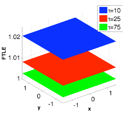
a) b)

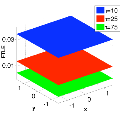
Figure 6: a) FTLE for the linear saddle point, (7), at different $\tau$.; b) FTLE for the linear elliptic point, (22), at different $\tau$.

In Figure 7 we compute the FTLEs for (27) for $\tau=25$ and $\tau=75$. The velocity field is integrable and expressed in action-angle coordinates. Therefore we know that the Lyapunov exponents are identically zero. However, since the velocity field is nonlinear, the approach to the limit is “nonuniform” in the sense that different trajectories show approach the limit at different rates. Consequently, Figure 7 shows “structure” in the FTLE fields (in contrast to our example linear velocity fields), but this structure will disappear in the infinite time limit. It is clear from the colour bar in Figure 7 that the FTLE are decreasing with $\tau$. Note that the smallest values for the FTLE appear near the invariant circle $I=\pm\frac{1}{\sqrt{3}}$, which correspond to the “twistless” invariant tori. It was shown in Beron-Vera et al. (2010) that twistless tori in integrable systems expressed in action-angle variables will have zero FTLE, for any time.

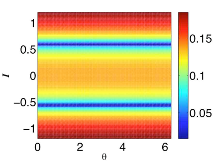
a) b)

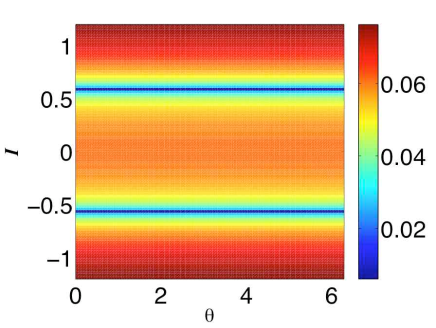
Figure 7: FTLE for (27). a) $\tau=25$; b) $\tau=75$.

2.3.2 Time Averages

In this section we will describe another approach for discovering phase space structure in dynamical systems that utilises time averages of certain functions along trajectories. Relating time averages to phase space structure is reminiscent of notions of ergodicity, and a general framework that has been used in the context of fluid flows (among other applications) is the ergodic decomposition. This approach was developed in Malhotra et al. (1998); Poje et al. (1999); Mezic and Wiggins (1999), and is based on fundamental work of Rokhlin (1966). Superficially, this approach appears to have some similarity to the method of Lagrangian descriptors. We will explain that this is not the case, and consider the application for the linear saddle (7), where this approach fails in several aspects.

We begin by giving a very brief description of the method. The setting is that of smooth ergodic theory. We have a compact domain, $A$, and a differentiable dynamical system defined on $A$ possessing an invariant measure. The dynamical system can be either discrete time, i.e. a map, or continuous time, i.e. a flow, and by “flow” we mean the precise mathematical definition as a one-parameter group of transformations of $A$. We denote by $L^{1}(A)$ the space of scalar valued functions on $A$ having the property that the integral of its absolute value over $A$ exists. It is essential that the Birkhoff ergodic theorem is applicable. In particular, we require that the time average of functions $f\in L^{1}(A)$ along trajectories of the dynamical system exist for almost all (with respect to the invariant measure) initial conditions in $A$, and we point out that by “time average” we mean infinite time average (as in the statement of the Birkhoff ergodic theorem).

Suppose we choose $f\in L^{1}(A)$, and consider the function on $A$ defined by the time average of $f$ along all possible trajectories in $A$. It can be shown that the level sets of this function are invariant sets with respect to the dynamics. Now suppose we have an inner product on $A$ and we are able to choose a set of mutually orthogonal functions, $\{f_{i}\},\,i\in\mathbb{N}$, having the property that the set of all possible linear combinations of the $\{f_{i}\}$ are dense in $L^{1}(A)$. For each $f_{i}$, we consider the function of $A$ given by the time average of trajectories through initial points in $A$, which we denote by $f^{*}$. Finally we consider the “joint level sets” that are constructed by considering the intersections of all level sets of all of the $f^{*}$. This collection of “joint level sets” defines a partition of $A$, and the dynamical of each element of the partition is ergodic (the “ergodic partition”).

An essential tool used in this procedure is the Birkhoff ergodic theorem which requires compactness of the phase space as an essential ingredient. Unfortunately, this theorem has not been proven for time dependent systems with general, aperiodic, time dependence. The theorem holds for maps and for time periodic and quasi periodic velocity fields. In the latter case the dimension of the system can be increased by considering time as an additional dependent variable in the definition of the velocity field. Since the velocity field is quasi periodic (of which periodicity is a special case) time is treated by including the independent (but finite) angles associated with each frequency component of the quasi periodic time dependence. In this way compactness is preserved (each included angular variable is compact) and the velocity field, in this higher dimensional setting, is autonomous and generates a flow on a compact space. For general, aperiodic time dependence transforming the problem to an autonomous setting in which compactness is preserved is generally not possible (see, e.g. Balibrea et al. (2010) for a recent review of the relevant issues for aperiodic time dependence).

Even though the Birkhoff ergodic theorem has not been proven for general aperiodic time dependence, the general approach suggested by the ergodic decomposition has proven fruitful, especially when the $f_{i}$ under consideration have a physical meaning (and this is not unlike the approach for constructing Lagrangian descriptors). In particular, the finite time average of the horizontal component of the velocity field has been shown to provide insight in the flow in numerous different situations by Mezic et al. (2010); Poje et al. (1999); Malhotra et al. (1998). For the general velocity field, (1), let $\mathbf{x}(t,t^{*},\tau)$ denote the trajectory satisfying $x(\mathbf{x}(t^{*},t^{*},\tau)=\mathbf{x}_{0}$ and let $v_{x}$ denote the $x$ component of the velocity field. Then the finite time average of $v_{x}$ along this trajectory is denoted by:

$$\mathbf{v}_{x}^{*}(\mathbf{x}_{0},t^{*},\tau)=\frac{1}{\tau}\int_{t^{*}}^{t^{*}+\tau}\mathbf{v}_{x}(\mathbf{x}(t,t^{*},\tau),t)dt$$ (28)

Since the integral is only over a finite length (in time) of the trajectory, conditions for its existence are relatively mild. However, the “meaning” of such results for such finite time averages is not a priori clear. The lack of a rigorous theoretical framework is similar to the situation for FTLEs. The typical approach is to compute the relevant quantities (e.g., (28)), “see” if the computations yield something “interesting”, and then to investigate further.

The linear velocity field (7) is defined on a non compact domain, thus the Birkhoff ergodic theorem does not apply to it, in the sense that it does not allow us to conclude that time averages along trajectories exist. Nevertheless, we can still compute the finite time averages along trajectories of physically interesting quantities in the spirit of the patchiness work described above. For this example the finite time average of the horizontal component of the velocity field can be explicitly computed. Taking $t_{*}=0,\,\lambda=1$, and denoting the finite time average of $v_{x}$ by $v_{x}^{*}$, we have:

$$v_{x}^{*}=\frac{x_{0}}{\tau}(exp(\tau)-1).$$ (29)

Clearly, the limit does not exist as $\tau\rightarrow\infty$. In figure 8 we plot the contours of (29) for $\tau=10$. It is also clear that the contour plot does not reveal the presence of the stable manifold nor invariant sets, despite the system, which is Hamiltonian, contains invariant sets defined by $H(x,y)=\lambda xy=c$ . The stable manifold of the hyperbolic trajectory at the origin is given by $x_{0}=0$. We see from (29) that the finite time average changes sign at $x_{0}=0$ (and this is true for any $\tau$). However, the derivative of (29) with respect to $x_{0}$ is smooth across $x_{0}=0$. Hence, the finite time average of the horizontal velocity component has no singular features that would indicate the presence of material curves. A reason for this behaviour is that general finite time averages do not require that the integrand is non-negative along trajectories, which is an essential requirement for Lagrangian descriptors, and motivation for this was given in the heuristic argument. Typically integrals of oscillating quantities along trajectories lead to a distorted output which makes interpretation of the results, in terms for phase space structure, difficult. In certain cases it was noted in Poje et al. (1999) that for increasing averaging time oscillations could lead to average velocities that approached zero everywhere, and as a consequence, in this limit any spatial structure is completely lost.

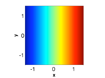
Figure 8: Integral of the horizontal component of the velocity along trajectories of the linear saddle point (7) for $\tau=10$.

2.4 Application to the Forced Duffing Oscillator

In this section we will discuss further the ability of Lagrangian descriptors to highlight manifolds. Also we will compare and contrast the behavior of Lagrangian descriptors with FTLEs and time averages of velocity components along trajectories using a familiar, but much more complicated nonlinear system –the forced Duffing equation:

$$\dot{x} = y,$$

$$\dot{y} = x-x^{3}+\varepsilon f(t),$$ (30)

We will consider three cases.

Integrable case.

In this case we take $\epsilon=0$ in (30). The phase space structure of the resulting system is well-known. The system has a hyperbolic fixed point at the origin connected by a symmetric pair of homoclinic orbits. The region inside and outside the homoclinic orbits consist of continuous families of periodic orbits, and correspond to elliptic regions.

Periodically time dependent case.

For this case we set $\varepsilon=0.1$ and $f(t)=\sin(t)$ (30). The system has a hyperbolic periodic trajectory near the origin, referred to as a distinguished hyperbolic trajectory, or DHT (see Mancho et al. (2003); Madrid and Mancho (2009); Ide et al. (2002)).

Aperiodically time dependent case.

The aperiodically time dependent forcing, $f(t)$, has the form shown in figure 9, which his obtained from a trajectory of the Duffing equation in a chaotic regime. We have chosen $\varepsilon=0.15$, which results in an amplitude of the time dependence that is, roughly, and order of magnitude smaller that the time periodic case considered above. In this case the system also has a hyperbolic trajectory near the origin.

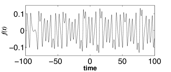
Figure 9: The time series of the function $f(t)$ corresponding to aperiodic time dependence for the Duffing Equation.

Singular Features of the Contour Plots of Lagrangian Descriptors.

In our study of the linear saddle in Section 2.1.1 we argued that Lagrangian descriptors had two important properties. 1) They depend on the time of integration $\tau$. 2) After a certain convergence time they display “singular contours” that correspond to the stable and unstable manifolds of hyperbolic trajectories. By “singular contours”, we mean that the Lagrangian descriptor is a function lacking regularity, either because the Lagrangian descriptor is itself discontinuous across the manifolds (we will see this is the case in Section 3) or because its derivative transverse to the manifolds is discontinuous. Here we will show that these two properties also hold for the cases of the forced Duffing equation that we have considered. In figure 10 we show the stable and unstable manifolds of the hyperbolic trajectory and contours of the function $M_{1}$ for $\tau=2$ and $\tau=10$. For both cases we see that the contours of $M_{1}$ converge to the stable and unstable manifolds.

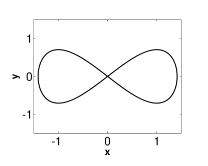
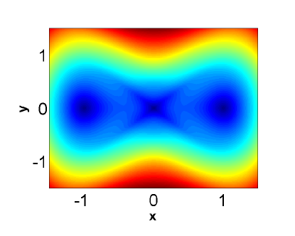
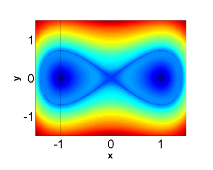
a) d)
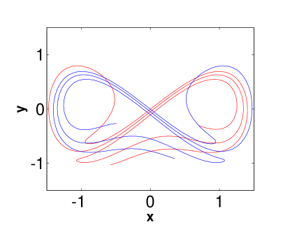
b) e)
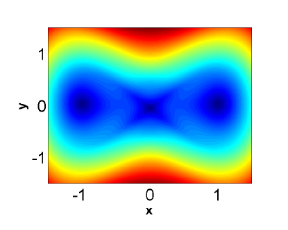
c) f)

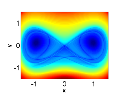
Figure 10: For the integrable case: a) the stable and unstable manifolds of the hyperbolic fixed point; b) contours of $M_{1}$ for $\tau=2$; c) contours of $M_{1}$ for $\tau=10$. For the periodically forced Duffing equation: d) Segments of the stable and unstable manifolds of the hyperbolic trajectory near the origin ; e) contours of $M_{1}$ for $\tau=2$; f) contours of $M_{1}$ for $\tau=10$.

Figure 11 further illustrates how singular features of the contours of $M_{1}$ correspond to stable and unstable manifolds of hyperbolic trajectories. The figure shows values of $M_{1}$ along the vertical line shown in Figure 10c). We see that the value of $M_{1}$ “change abruptly” at the locations of the manifolds. Discontinuities in the derivative of $M_{1}$ quantify the notion of “abrupt change” of $M_{1}$. The latter are illustrated in the dashed line in the figure.

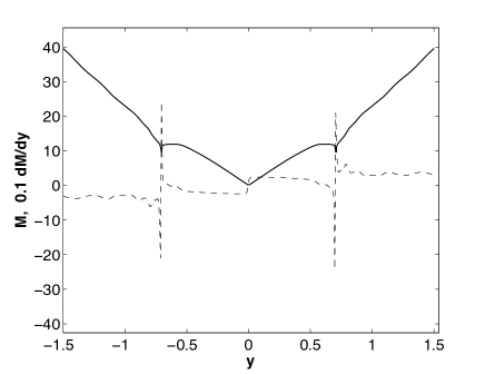
Figure 11: The black solid line represents the function $M_{1}$ vs $y$ at a fixed $x$. $M_{1}$ along the vertical black line shown in Figure 13c). Abrupt changes in $M_{1}$, occurring at the location of the manifolds, correspond to discontinuities of the derivative of $M_{1}$. The dashed line represents 0.1 times the derivative of $M_{1}$ with respect to $y$.

In figure 12 a) we show segments of the stable and unstable manifolds of the hyperbolic trajectory near the origin. In figure 12 b) we show the same manifolds overlaid with the contours of $M_{1}$ computed for $\tau=10$. The manifolds align well with the “singular contours” of $M_{1}$.

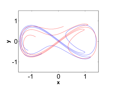
a) b)

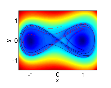
Figure 12: The aperiodically time dependent case. a) The stable and unstable manifolds of the hyperbolic trajectory near the origin. b) An overlay of the stable and unstable manifolds of the hyperbolic trajectory near the origin with the contours of the $M_{1}$. The manifolds and $M_{1}$ are computed for $\tau=10$.

Lagrangian Descriptors vs FTLE.

In figure 13 we show the stable and unstable manifolds of the hyperbolic trajectory near the origin (left most column), the forward time FTLEs (middle column) and the contours of the Lagrangian descriptor $M_{1}$ for the three cases, and all for $\tau=10$. In all cases the “singular” contours of $M_{1}$ approximate the manifolds much better than the contours of the forward FTLE, since although the forward FTLE only captures the stable manifold of the hyperbolic trajectory near the origin, it displays ridges which are artifacts in the FTLE field that have no Lagrangian interpretation, and that are not present on the contour plots of $M_{1}$.

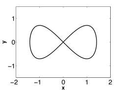
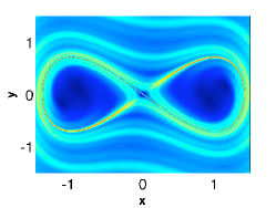
a) b) c)

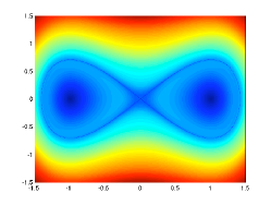
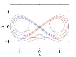
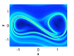
d) e) f)

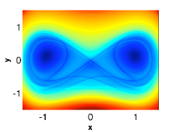
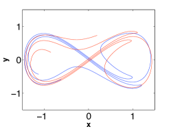
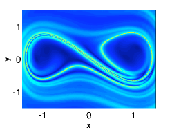
g) h) i)

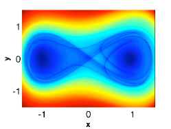
Figure 13: For the integrable Duffing equation: a) the stable and unstable manifolds of the hyperbolic fixed point; b) forward FTLE for $\tau=10$; c) contours of $M_{1}$ for $\tau=10$. For the periodically forced Duffing equation: d) segments of the stable and unstable manifolds of the hyperbolic trajectory near the origin computed for $\tau=10$ (and displayed at $t=0$); e) forward FTLE for $\tau=10$; f) contours of $M_{1}$ for $\tau=10$. For the aperiodically forced Duffing equation: g) segments of the stable and unstable manifolds of the hyperbolic trajectory near the origin computed for $\tau=10$ (and displayed at $t=0$); h) forward FTLE for $\tau=10$; i) contours of $M_{1}$ for $\tau=10$.

Lagrangian Descriptors in Elliptic Regions.

Next we consider the behaviour of several Lagrangian descriptors in “elliptic regions” (cf. the discussion of elliptic and hyperbolic regions in Section 2) for both the periodic and aperiodically time dependent cases. The elliptic region that we consider consists of the region enclosed by the left hand homoclinic orbit in the $\epsilon=0$ case (but we consider the behaviour of the Lagrangian descriptors in this region for the periodic and aperiodically time dependent cases).

We first consider the Lagrangian descriptors $M_{5}$ and $M_{2}$ in the periodically time dependent case. Figure 14 a) and b) shows the contours of these Lagrangian descriptors computed for $\tau=70$. The contours of each Lagrangian descriptor show a smooth structure near the centre of the elliptic region. This is not surprising since for a “weak” time-periodic perturbation of an integrable system we expect “most” of the closed trajectories to be preserved as (two-frequency) Kolmogorov-Arnold-Moser tori. This would imply that trajectories starting “close” to each other would have a similar past and future on the time interval $(t-\tau,t+\tau)$. Outside this smooth region the contours of $M_{5}$ and $M_{2}$ reveal a more complex structure. This “complex structure” appears to be associated with strong mixing. This suggests that $\tau$ may be a useful parameter for quantifying the notion of “finite time mixing”, but making this notion precise requires further research. Practically, the notion of “finite time mixing” is very important in applications, and lies outside the scope of notions of mixing in traditional ergodic theory.

Next we consider the aperiodically time dependent case in the same region. In this case the isolated region of “trapped” trajectories shown in Figure 14 a) and b) is “broken” as it is “invaded” by segments of the stable and unstable manifolds of the hyperbolic trajectory near the origin, as shown in Figure 14 c) and d) for the Lagrangian descriptors $M_{3}$ and $M_{4}$ (more details are evident from the contours of $M_{3}$). Although not shown, we note that the Lagrangian descriptors $M_{1}$, $M_{2}$ and $M_{5}$ give results similar to those of $M_{4}$ and $M_{3}$ in this case.

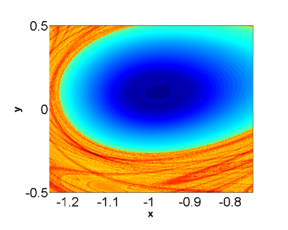
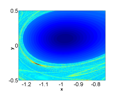
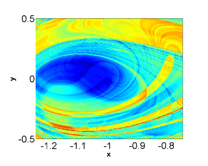
a) b) c) d)

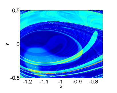
Figure 14: Contour plots of the of Lagrangian descriptors in the region corresponding to that enclosed by the left hand homoclinic orbits for $\epsilon=0$. Panels a) $M_{5}$; b) $M_{2}$ correspond to the periodically time dependent case. Panels c) $M_{3}$; d) $M_{4}$ correspond to the aperiodically time dependent case. The Lagrangian descriptors are computed for $\tau=70$.

Time Averages of Velocity Components.

We now return to the issues raised in Section 2.3.2. In particular, we compute the finite time average of the horizontal component of the Duffing equation, following (28), for the three different time dependencies that we are considering.

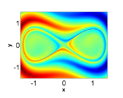
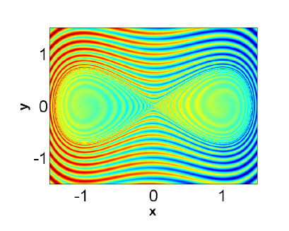
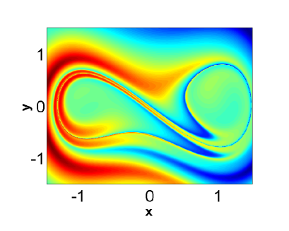
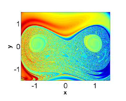
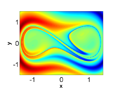
a) b) c) c) e) f)

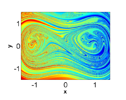
Figure 15: Contours of the finite time average of the horizontal component of the Duffing Equation along trajectories; The integrable case ($\epsilon=0$) for a) $\tau=10$; b) $\tau=70$; the periodic case for c) $\tau=10$ d) $\tau=70$; the aperiodic case for e) $\tau=10$; f) $\tau=70$.

The results are shown in figure 15, where the time averages are computed in each case for $\tau=10$ and $\tau=70$. For each time dependence we see similar behavior. For the smaller time we see “a hint” of structure that bears some resemblance to “fattened” versions of short segments of manifolds of the unstable manifold of the hyperbolic trajectory. For the longer time the contours of the finite time average of the horizontal component of velocity develop a more complex spatial structure that obscures the underlying unstable manifold structure of the hyperbolic trajectory.

3 Applications to time dependent 3D flows

In this section we show that Lagrangian descriptors can also provide accurate information on the stable and unstable manifolds of hyperbolic trajectories in three dimensional (3D) time dependent flows. Computation of the stable and unstable manifolds of hyperbolic trajectories in aperiodically time dependent flows was discussed in Branicki and Wiggins (2009), where an algorithm for their calculation was developed and several “benchmark” examples were considered. The particular example that we will consider is the perturbed Hill’s spherical vortex, which we will take as a benchmark for the performance of our methods in 3D. We give a brief description of the velocity field. More details on the background of Hill’s spherical vortex can be found in Branicki and Wiggins (2009).

The velocity field, ${\bf v}$, has the general form:

$${\bf v}=H(x,y,z)+S(x,y,z,t)$$

where $H(x,y,z)$ is given by:

$$H_{x} = (u_{r}\sin\Theta+u_{\Theta}\cos\Theta)\cos\Phi,$$ (31)

$$H_{y} = (u_{r}\sin\Theta+u_{\Theta}\cos\Theta)\sin\Phi,$$ (32)

$$H_{z} = (u_{r}\cos\Theta-u_{\Theta}\sin\Theta),$$ (33)

Here:

$$r=\sqrt{x^{2}+y^{2}+z^{2}},\quad\Theta=\arccos(z/r),\quad\Phi=\arccos(x/\sqrt{x^{2}+y^{2}})$$

$$u_{r}=\left\{\begin{array}[]{ll}U(1-a^{3}/r^{3})\cos\Theta,&{\rm if}\,\,r\geq a,\\ -\frac{3}{2}U(1-r^{2}/a^{2})\cos\Theta,&{\rm if}\,\,r<a,\end{array}\right.\\ u_{\Theta}=\left\{\begin{array}[]{ll}-U(1+a^{3}/(2r^{3}))\sin\Theta,&{\rm if}\,\,r\geq a,\\ \frac{3}{2}U(1-2r^{2}/a^{2})\sin\Theta,&{\rm if}\,\,r<a,\end{array}\right.$$ (34)

The matrix $S$ is given by:

$$S=\mathcal{A}(t)\cdot\delta^{-1}\left[\begin{array}[]{ccc}\alpha(t)&0&0\\ 0&\beta(t)&0\\ 0&0&\gamma(t)\end{array}\right]\cdot\delta\cdot\left[\begin{array}[]{c}x\\ y\\ z\end{array}\right]$$

where $\delta$ is the orthogonal matrix:

$$\delta=\left[\begin{array}[]{ccc}cos\psi\cos\varphi-\sin\psi\cos\theta\sin\varphi&\cos\psi\sin\varphi+\sin\psi\cos\theta\cos\varphi&\sin\psi\sin\theta\\ -\sin\psi\cos\varphi-\cos\psi\cos\theta\sin\varphi&-\sin\psi\sin\varphi+\cos\psi\cos\theta\cos\varphi&\cos\psi\sin\theta\\ \sin\theta\sin\varphi&-\sin\theta\cos\varphi&\cos\theta\end{array}\right],$$

and $A(t)$ is the time dependent function:

$$\mathcal{A}(t)=(0.3+0.27\sin(3.3t))\exp(-(t-6)^{2}/2.5^{2}).$$ (35)

Additionally:

$$\theta=0.5+0.05\sin(2t),\;\varphi=5t,\;\psi=0$$

and

$$\alpha(t)=-0.5,\;\beta(t)=-0.5\,\,{\rm and}\,\,\gamma(t)=1.$$

For $\mathcal{A}(t)=0$ the flow is steady and has hyperbolic stagnation points at:

$$h_{1} = (0,0,-a),$$

$$h_{2} = (0,0,a),$$ (36)

where $h_{1}$ has a one dimensional stable manifold and a two dimensional unstable manifold, and $h_{2}$ has a two dimensional stable manifold and a one dimensional dimensional manifold. In Branicki and Wiggins (2009) numerical algorithms are used to show that when $\mathcal{A}(t)$ increases from $0$ to the expression in (35), $h_{1}$ and $h_{2}$ “continue” to be hyperbolic (time-dependent) trajectories, denoted $\gamma_{1}$ and $\gamma_{2}$, respectively, and at each instant of time $\gamma_{1}$ has a one dimensional stable manifold and a two dimensional unstable manifolds, and $\gamma_{2}$ has a two dimensional stable manifold and a one dimensional stable manifold. The unstable manifold at $t=5.3$ with $U=2$ and $a=2$ computed as in Branicki and Wiggins (2009) is displayed in Figure 16a).

We now illustrate the performance of Lagrangian descriptors for this three dimensional, aperiodically time dependent example. Figure 16b) and c) show respectively the intersection of the unstable manifold with vertical (at $y=-0.3$) and horizontal (at $z=0$) cross sections of $M_{2}$ obtained under the same conditions. The agreement is excellent.

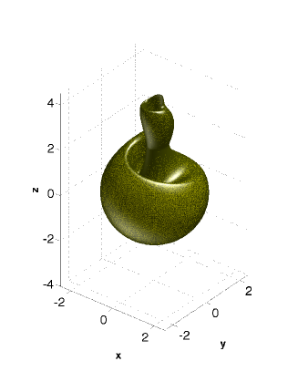
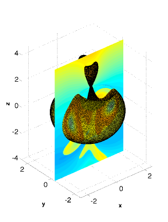
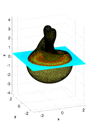
Figure 16: a) The two dimensional unstable manifold of $\gamma_{1}$ is shown at $t=5.3$ for $U=a=2$ (image courtesy of M. Branicki); b) the intersection of the unstable manifold with a vertical cross section of $M_{2}$ obtained at $y=-0.3$ and $t=5.3$ for $\tau=10$; c) the intersection of the unstable manifold with a horizontal cross section of $M_{2}$ obtained at $z=0$ and $t=5.3$ for $\tau=10$

The Lagrangian descriptor $M_{2}$ provides many details on the Lagrangian structure of the flow as Figure 17a) confirms. It shows the results on the vertical section displayed in Figure 16b) obtained with $\tau=10$. Similar slices are displayed in Figure 17b) for the descriptor $M_{1}$. The output is similar to $M_{2}$, but with a lower contrast which make more difficult the visualization. The structure is clean and sharp in contrast to that provided by methods discussed next. FTLE computations, similarly to what happened in the 2D case, distorts the image by introducing numerous structures that do not have Lagrangian interpretation. The output of forwards and backwards FTLE is displayed in figure 17c) and d) confirms this extreme. Alternative averages as those proposed in section 2.3 provide the output shown in figure 17e) and f). These averages also present spurious structures that distort the output and blur the true Lagrangian information.

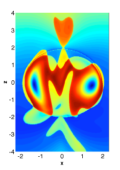
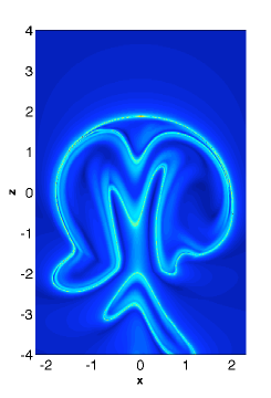
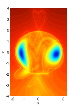
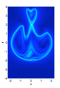
a)c) e)
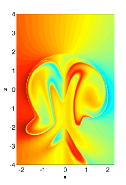
b)d)f)

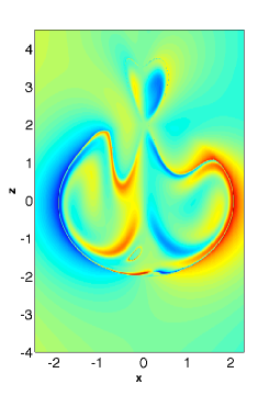
Figure 17: a) Evaluation of $M_{2}$ on the vertical plane $(x,y=-0.3,z)$ at $t=5.3$ for $\tau=10$; b) the structure provided by $M_{1}$ also on the vertical plane $(x,y=-0.3,z)$ at $t=5.3$ for $\tau=10$; c) the forward FTLE field on the vertical plane $(x,y=-0.3,z)$ at $t=5.3$ for $\tau=10$; d) the backward FTLE on the vertical plane $(x,y=-0.3,z)$ at $t=5.3$ for $\tau=10$; e) the forward average of the horizontal component of the velocity; f) the backward average of the horizontal component of the velocity.

4 Application of Lagrangian Descriptors to Velocity Fields Defined as Data Sets

In this section we discuss the performance and application of Lagrangian descriptors to velocity fields defined as data sets. In particular, we will consider the finite time data set obtained from the numerical simulation of a wind driven, quasi-geostrophic (QG) 3-layer model in a rectangular basin geometry on a $\beta$-plane (Rowley (1996)). The basic circulation pattern in the upper layer is an unsteady double-gyre structure, i.e. a counterclockwise gyre in the north and a clockwise gyre in the south separated by a jet. The velocity data set is obtained on a 1000 km $\times$ 2000 km rectangular domain with spatial and temporal resolutions of 12.5 km $\times$ 12.5 km and 2 hours (although the data is only saved every 24 hours), respectively, and spans over 4000 days. The 4000 day interval of the data set is considered after the fluid is started from rest and allowed to spin up for 25000 days. More details of the specific parameters used and the numerical method used for solving the QG equations can be found in Rowley (1996) or Coulliette and Wiggins (2001).

We have chosen this data set because it is aperiodic and results on the computation of distinguished hyperbolic trajectories (DHTs) and their stable and unstable manifolds have previously been reported in Mancho et al. (2004, 2006c); Madrid and Mancho (2009). In particular, we choose three hyperbolic trajectories that have previously been identified in a range of days between 0 and 900 in Mancho et al. (2004, 2006c). Figure 18 shows one of these DHTs located in the northern gyre, which has been shown to possess the “distinguished property” in the interval between 120 days and 300 days (more details on this can be found in Madrid and Mancho (2009)). Beyond this time interval the trajectory still exists, but it no longer has the “distinguished” property. The loss of the distinguished property has been linked in Madrid and Mancho (2009) with the loss of hyperbolicity. We remark that in complex time varying geophysical flows one frequently observes trajectories whose finite time stability characteristics change from hyperbolic to elliptic, and vice versa. This is a particularly challenging phenomenon for the dynamical systems approach and has been discussed in Branicki and Wiggins (2010); Mancho et al. (2006b); Madrid and Mancho (2009); Branicki et al. (2011).

Figures 19a) and b) show the results of the direct computation of the stable manifold for two of the DHTs and the unstable manifold for the remaining DHT for days 290 and 320 using the algorithms described in Mancho et al. (2004). This figure also shows contour plots for a selection of Lagrangian descriptors computed for $\tau=150$.

We note that there is an essential difference between the figures showing the direct computation of DHTs and their stable and unstable manifolds and the contours of Lagrangian descriptors. In order to compute manifolds of DHTs, we must first identify and compute the DHTs. Lagrangian descriptors, on the other hand, compute the stable and unstable manifolds for all DHTs present during a chosen time interval, i.e., there is no need to identify the DHTs a priori.

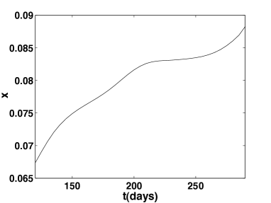
a) b)

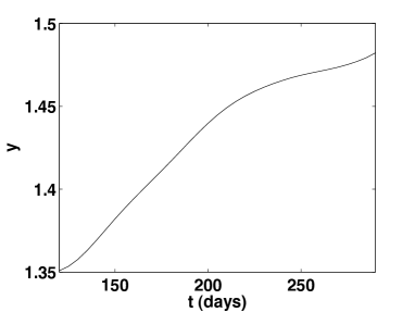
Figure 18: The time evolution of a DHT; a) the $x$-coordinate; b) the $y$-coordinate. Units are in thousands of kilometers.

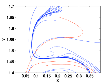
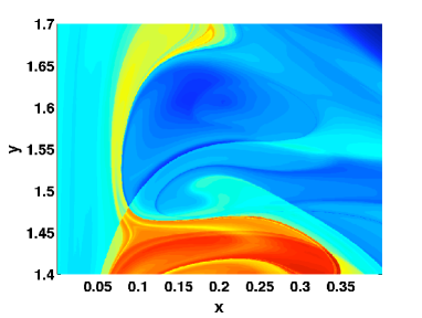
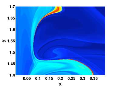
a) b)
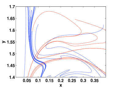
c) d)
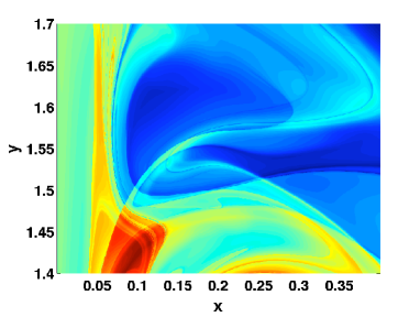
e) f)

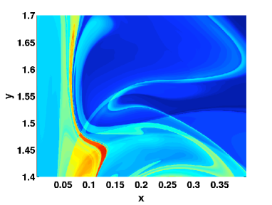
Figure 19: Pieces of stable manifold (blue) for two DHTs and and unstable manifolds (red) of the remaining DHT shown on a) day 290; b) day 320. Contour plots for a selection of Lagrangian descriptors evaluated over the quasigeostrophic flow with $\tau=150$. c) $M_{3}$ at day 290; d) $M_{1}$ at day 320; e) $M_{5}$ at day 290; f) $M_{2}$ at day 320. The units on the axis are in thousands of kilometers.

Typically the Lagrangian structure revealed by different Lagrangian tools contains more details for longer integration times $\tau$. However, it is also of much interest in applications to obtain accurate Lagrangian information for small $\tau$. We will address how Lagrangian descriptors perform in this context, as well as make comparisons with the performance of FTLEs, by studying the convergence rate of different Lagrangian descriptors with $\tau$ towards the singular lines that reveal the Lagrangian structure of the flow. Our attention is not on the manifold structure for a large spatial region, but on the stable and unstable subspaces tangent to the stable and unstable manifolds of a particular DHT. We remark that these subspaces are related to the also called Lyapunov vectors Legras and Vautard (1996) that indicated dispersive directions in the fluid flow, backwards and forwards in time.

We place our study at day 130, far from the transition of the DHT. Figure 20 shows the stream function on this date with the position of the DHT indicated at (70.631, 1357.660) km. We use Lagrangian descriptors to approximate the stable and unstable subspaces of the DHT as follows. We consider a “small” circle centred at the DHT. In particular, we consider the circle centred at the DHT parametrized as $(r\cos(\alpha),r\sin(\alpha))$ and of radius $r=1.5$ km. We then compute the Lagrangian descriptor for trajectories starting in this circle for different $\tau$, and consider the singular contours of the Lagrangian descriptor near the DHT. These are approximations to the stable and unstable subspaces of the DHT.

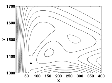
Figure 20: Stream function of the quasigeostrophic model at day 130. The position of a DHT at this day is marked with a circle. The units on the axis are in kilometers.

Figure 21 summarizes the convergence of different Lagrangian descriptors towards the stable and unstable subspaces of the DHT at day 130. The angle positions of the stable and unstable subspaces are marked with vertical lines. Panel 21a) shows $M_{1}$, $M_{3}$ and $M_{5}$ versus $\alpha$ for $\tau=45$, which for this specific vector field is not a large value. At this stage singular features are only developed by $M_{3}$, which has been obtained based on the magnitude of acceleration and using $\gamma=1/2$ in the exponent of its definition. The Lagrangian descriptor $M_{1}$ shows a slower convergence towards the subspace aligned along $\alpha=2.032$ and $\alpha=2.032+\pi/2$. The features displayed by $M_{5}$ are not yet sharp enough at this stage. Panel 21b) confirms a finer structure for $\tau=65$ for the Lagrangian descriptor $M_{3}$. The Lagrangian descriptors $M_{4}$ and $M_{5}$ perform worse at this stage, while the output of $M_{1}$ and $M_{2}$ is similar to that of $M_{3}$. Panel 21c) shows $M_{2}$ and $M_{4}$ at $\tau=95$, when convergence has been reached for all of the Lagrangian descriptors considered.

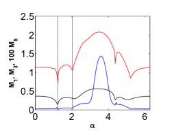
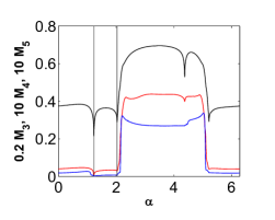
a) b) c)

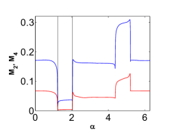
Figure 21: a) Lagrangian descriptors $M_{1}$ (black), $M_{3}$ (red) and $100\times M_{5}$ (blue) versus $\alpha$ for $\tau=45$; b) descriptors $0.2\times M_{3}$ (black), $10\times M_{4}$ (red) and $10\times M_{5}$ (blue) versus $\alpha$ for $\tau=65$; c) $M_{2}$ (blue) and $M_{4}$ (red) versus $\alpha$ for $\tau=95$

These results indicate that the Lagrangian descriptor $M_{3}$ for this example performs the best in the sense that it indicates the subspaces for smaller $\tau$. It is followed by $M_{1}$, $M_{2}$, and $M_{5}$, respectively. The Lagrangian descriptor $M_{4}$, also develop sharp features along the same structures, but it requires longer time intervals of integration for the situations considered here.

Figure 22 contrasts the ability of FTLE to locate the stable and unstable subspaces of the DHT with that of the Lagrangian descriptors. For comparison purposes, we choose $M_{3}$. For reference, the angle positions of the stable and unstable subspaces are marked with vertical lines. Panel 22a) shows the forward and backward FTLE and $M_{3}$ versus $\alpha$ for $\tau=45$. The Lagrangian descriptor $M_{3}$ is represented by a blue line. Its sharp features mark accurately the position of the stable and unstable subspaces. The forward FTLE, represented by the thin black line, at this stage presents pronounced features, although not yet sharp. Deviations from the correct position of the stable subspace are significant. and the performance of forward FTLE is clearly lower than that of $M_{3}$. The backward FTLE, represented by the red line, accurately detects the unstable subspace with a similar performance to that of $M_{3}$. Panel 22b) presents results for $\tau=65$. However, deviations of the forward FTLE field (black line) with respect to the stable subspace are still noticeable in this panel. Panel 22c) confirms that at $\tau=95$ both FTLE and Lagrangian descriptors perform well at locating the angles of the stable and unstable subspaces.

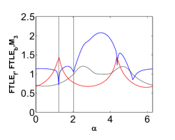
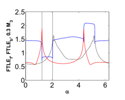
a) b) c)

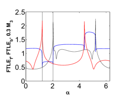
Figure 22: a) Forwards FTLE (black), backwards FTLE (red) and $M_{3}$ (blue) versus $\alpha$ for $\tau=45$; b) forwards FTLE (black), backwards FTLE (red) and $M_{3}$ (blue) versus $\alpha$ for $\tau=65$; c) forwards FTLE (black), backwards FTLE (red) and $M_{3}$ (blue) versus $\alpha$ for $\tau=95$

5 Computational performance

Computationally the evaluation of Lagrangian descriptors offer numerous advantages in comparison with the computation of FTLE, as we discuss next. We explain these advantages in 2D flows, but the argued aspects are enhanced in 3D flows. Calculation of FTLE requires the evaluation of the gradient of the flow map, which is numerically realized by expression (49) in the Appendix. As indicated there for obtaining the $\sigma$ field at a grid point ${\bf x}^{*}_{i,j}$ in a 2D flow it is requested to integrate the dynamics of four neighbour points ${\bf x}^{*}_{i-1,j},{\bf x}^{*}_{i+1,j},{\bf x}^{*}_{i,j-1},{\bf x}^{*}_{i,j+1}$ which must be a small distance $\epsilon$ from ${\bf x}^{*}_{i,j}$ in order to keep valid expression (49) in the range of integration $(t^{*},t^{*}+\tau)$. Thus in order to be accurate, the numerical approach (49) must keep a balance between the distance of grid points $\epsilon$ and the integration time $\tau$. These parameters must be appropriately tuned. This tuning is not necessary in the computation of the Lagrangian descriptors, thus making their computation more direct. On the other hand if the grid size in which the $\sigma$ field is evaluated is bigger than $\epsilon$, then for obtaining its value in a point ${\bf x}^{*}_{i,j}$ expression (49) indicates that four integrations are necessary, while Lagrangian descriptors require only one. This makes Lagrangian descriptors computationally much more efficient, specially in geophysical flows given as finite time datasets, because in them integrations require interpolations which are computationally expensive. Some approaches compute FTLE taking $\epsilon$ as the grid size in which the $\sigma$ field is evaluated. In this case integrations of neighbours are stored to prevent multiple performaces of the same trajectory, and then only one integration per point ${\bf x}^{*}_{i,j}$ is requested. However this approach has also several computational disadvantages with respect to the use of Lagrangian descriptors. One is that it is harder to program because the evaluation of the FTLE at each point requires access to stored information, and the second is that the grid size is doomed to be small enough to keep expression (49) accurate in the range $(t^{*},t^{*}+\tau)$. This size can be much smaller that the grid size required to have a smooth representation for the Lagrangian descriptor, and in this case the computation of FTLE is again more expensive.

Another difference between Lagrangian descriptors and FTLE is that the former provide the stable and unstable manifolds simultaneously in the same output, while the latter require post-processing of the results into one picture. In the post-processing of the output typically the results are ’filtered’ by using a threshold in the field values (see Branicki and Wiggins (2010)) and in this processes spurious structures may be removed. In the case of Lagrangian descriptors an accurate image of the manifold features is obtained without the need of any ’filtering’ process. de la Cámara et al. (2012) have demonstrated that in applications having both the stable and unstable manifolds simultaneously in one picture is an interesting feature that is essential for the successful analysis of transport events.

6 Conclusions and Outlook

In this paper we have proposed a general method for revealing geometrical structures in phase space that is valid for aperiodically time-dependent dynamical systems. The central quantities in our method are referred to as Lagrangian descriptors and are based on finite time integrals of some positive, bounded intrinsic geometrical or physical properties of the dynamical system along trajectories. In particular, these properties are integrated forward and backward in time on some interval $(t-\tau,t+\tau)$. In this way, the Lagrangian descriptors have the capability of revealing both the stable and unstable manifolds in the same calculation. We have shown that the convergence to geometrical structures of the dynamical system requires the use of a long enough $\tau$. For $\tau$ values below a threshold, which depends on each particular dynamical system, the pattern provided by the Lagrangian descriptors is far from the geometrical structures. However beyond that threshold, for increasing $\tau$, the output of the Lagrangian descriptors becomes more and more complex, revealing more details of the geometrical structures of the dynamical system. We have given an analytical justification for these observations for the benchmark case of a linear vector field having a hyperbolic saddle point.

In all examples that we have considered we have carried out simultaneous comparisons of FTLEs and finite time averages of components of the vector field along trajectories with Lagrangian descriptors. We have shown that Lagrangian descriptors provide superior performance in all cases, in the sense that they more accurately reveal the geometrical structures and they require a shorter time to converge to the geometrical structures. For example, we have shown that FTLE give spurious structures for the integrable Duffing equation and fail completely to provide any structure for the linear saddle. Finite time averages of the horizontal component of the vector field exhibit the same deficiencies as FTLEs for these particular two examples. We have also shown that Lagrangian descriptors accurately provide the geometrical structures for a three dimensional flow. We have compared these results to results obtained from FTLE calculations and finite time averages of a component of the vector field along trajectories and we have seen that Lagrangian descriptors provide a more accurate representation of the geometrical features of the flow than these techniques provide. We have examined the issue of the convergence time to the stable and unstable subspaces of a DHT for a velocity field given as a data set and have shown that Lagrangian descriptors converge more rapidly to these subspaces than FTLE. This is promising from the applications point of view, in which reductions for the forecast time of the velocity field is desirable. Lagrangian descriptors can give more accurate predictions with less information in time. Finally we have shown that computationally Lagrangian descriptors provide several advantages over FTLE. In general, their use leads to a reduction in CPU requirements by a factor of 4, their implementation in code is simpler, and they require no ”parameter tuning”. Moreover, Lagrangian descriptors provide both the stable and unstable manifolds in one output. In order to achieve this with FTLE post-processing of the stable and unstable is required in order to combine the two outputs into one picture at the same time.

Appendix A Numerical computation of Lagrangian descriptors

In this appendix we describe the numerical computation of general Lagrangian descriptors:

$$M({\bf x^{*}},t^{*})_{{\bf v},\tau}=\int^{t^{*}+\tau}_{t^{*}-\tau}\mathcal{F}({\bf x}(t))\,dt.$$ (37)

where $\mathcal{F}({\bf x}(t))$ is a positive bounded scalar representing a geometrical or physical property that is evaluated along a trajectory. This scalar properties introduced in this paper depend on vector quantities such as velocity, acceleration, the time derivative of acceleration or combinations of these quantities (e.g. as in the example using curvature). For example, for the Lagrangian descriptor $M_{1}$, Eq. (2), is evaluated by integrating the function $\|{\bf v}({\bf x}(t),t)\|$ along a trajectory, $\bf{x}(t),\,{\bf x}(t^{*})={\bf x}^{*}$ from from $t^{*}-\tau$ to $t^{*}+\tau$.

Geometrically, the computation of $M_{1}$ is equivalent to evaluating the area $A$ below the graph $\|{\bf v}({\bf x}(t),t)\|$ in the specified time interval. The area $A$ is obtained from the following one dimensional dynamical system:

$$\frac{dY}{dt}=\|{\bf v}({\bf x}(t),t)\|.$$ (38)

For the initial condition $Y(t^{*})=0$, the area $A$ is given by the value of $Y$ at $t^{*}+\tau$ minus the value of $Y$ at $t^{*}-\tau$ , i.e., $Y(t^{*}+\tau)-Y(t^{*}-\tau)=A$.

The integration of the system (38) is performed with a 5th order variable time step Runge-Kutta method, in particular with the subroutine rkqs described in Press et al. (1999). A peculiarity of this differential equation is that it depends on $t$ both explicitly and implicitly through the trajectory of (1). A Runge-Kutta step from $t_{0}$ to $t_{1}$ applied to Eq. (38) requires evaluating $\|{\bf v}\|$ along trajectories of (1) at intermediate steps $t_{0}+\Delta t$. To this end the argument ${\bf x}(t)$ that must be passed to $\|{\bf v}\|$ at time $t_{0}+\Delta t$ must be obtained by evolving the trajectory of (1) from ($t_{0},{\bf x}(t_{0})$) to ($t_{0}+\Delta t,{\bf x}(t_{0}+\Delta t)$). We remark that this adaptive method can be faster than the method proposed in Madrid and Mancho (2009) which is based on fixed time step integrations. Moreover, this method is quite versatile, since from one descriptor to another it is only the right hand side in Eq. (38) which needs to be modified.

In order to evaluate the entire family of descriptors presented in this paper three different types of vectors must be obtained: velocity, acceleration and the time derivative of acceleration. Once these are obtained individually, their combinations relevant to the particular type of descriptor of interest are straightforwardly computed. Velocity is a vector which is directly provided if Eqs. (1) are given; the others are obtained as we explain next. The general expression for ${\bf a}({\bf x},t)$ is as follows:

$${\bf a}({\bf x},t)=\frac{d{\bf v}}{dt}=\frac{\partial{\bf v}}{\partial t}+\frac{\partial{\bf v}}{\partial x}v_{x}+\frac{\partial{\bf v}}{\partial y}v_{y}$$ (39)

which is easily computed if there is an exact expression for the velocity field v. If the velocity field is given as a finite time data set, Eq. (39) is evaluated by providing a discrete version of the equation:

$${\bf a}=\frac{d{\bf v}}{dt}=\frac{d^{2}{\bf x}}{dt^{2}}$$ (40)

as follows:

$${\bf a}({\bf x}(t),t)=\frac{{\bf v}({\bf x}(t+h),t+h)-{\bf v}({\bf x}(t-h),t-h)}{2h}+\mathcal{O}(h^{2}).$$ (41)

The time derivative of the acceleration is given by:

$$\frac{d{\bf a}({\bf x},t)}{dt} = \frac{d}{dt}\frac{d{\bf v}}{dt}=\frac{\partial^{2}{\bf v}}{\partial t^{2}}+\frac{\partial^{2}{\bf v}}{\partial t\partial x}v_{x}+\frac{\partial{\bf v}}{\partial x}\frac{\partial v_{x}}{\partial t}+\frac{\partial^{2}{\bf v}}{\partial t\partial y}v_{y}+\frac{\partial{\bf v}}{\partial y}\frac{\partial v_{y}}{\partial t}+$$ (42)

$$\frac{\partial^{2}{\bf v}}{\partial x\partial t}+\frac{\partial^{2}{\bf v}}{\partial x^{2}}v_{x}+\frac{\partial{\bf v}}{\partial x}\frac{\partial v_{x}}{\partial x}+\frac{\partial^{2}{\bf v}}{\partial x\partial y}v_{y}+\frac{\partial{\bf v}}{\partial y}\frac{\partial v_{y}}{\partial x}+$$

$$\frac{\partial^{2}{\bf v}}{\partial y\partial t}+\frac{\partial^{2}{\bf v}}{\partial y\partial x}v_{x}+\frac{\partial{\bf v}}{\partial x}\frac{\partial v_{x}}{\partial y}+\frac{\partial^{2}{\bf v}}{\partial y^{2}}v_{y}+\frac{\partial{\bf v}}{\partial y}\frac{\partial v_{y}}{\partial y}.$$

If the velocity is supplied as a finite time data set, Eq. (42) is evaluated by providing a discrete version to the equation:

$$\frac{d{\bf a}}{dt}=\frac{d^{2}{\bf v}}{dt^{2}}.$$ (43)

which reads as follows:

$$\frac{d{\bf a}({\bf x}(t),t)}{dt}=\frac{{\bf v}({\bf x}(t+h),t+h)-2{\bf v}({\bf x}(t),t)+{\bf v}({\bf x}(t-h),t-h)}{2h}+\mathcal{O}(h^{2}).$$ (44)

For the results reported in this article Eqs. (41) and (44) are implemented where needed using $h=10^{-4}$.

Appendix B Computation of FTLE’s

In this appendix we give a brief discussion of the computation of FTLEs, following Lekien et al. (2007). The FTLE field is denoted by $\sigma_{t^{*}}^{\tau}({\bf x}^{*})$, and is computed from the maximum eigenvalue $\lambda_{\rm max}$ of the matrix $\Delta$:

$$\sigma_{t^{*}}^{\tau}({\bf x}^{*})=\frac{1}{\tau}\ln\sqrt{\lambda_{\rm max}(\Delta)},$$ (45)

where the matrix $\Delta$ is defined from the flow map, as we now describe. Consider a point ${\bf x}^{*}$ at time $t^{*}$, and let it be advected by the flow map, $\phi$, from $t^{*}$ to $t^{*}+\tau$:

$${\bf x}^{*}\to\phi^{t^{*}+\tau}_{t^{*}}({\bf x}^{*}).$$ (46)

The gradient of the flow map defines the matrix $N$:

$$N=\frac{d\phi^{t^{*}+\tau}_{t^{*}}({\bf x}^{*})}{d{\bf x}^{*}}$$ (47)

Using the convention that $N^{T}$ denotes the transpose of $N$, $\Delta$ is the symmetric matrix:

$$\Delta=N^{T}N$$ (48)

Note that in two dimensions the gradient of the flow map at a grid point ${\bf x}^{*}_{i,j}=(x_{i,j},y_{i,j})$ can be computed central differences as follows (see Shadden (2005)):

$$\frac{d\phi^{t^{*}+\tau}_{t^{*}}({\bf x}^{*})}{d{\bf x}^{*}}\Bigg{|}_{{\bf x}^{*}_{i,j}}=\left(\begin{array}[]{cc}\frac{x_{i+1,j}(t^{*}+\tau)-x_{i-1,j}(t^{*}+\tau)}{x_{i+1,j}(t^{*})-x_{i-1,j}(t^{*})}&\frac{x_{i,j+1}(t^{*}+\tau)-x_{i,j-1}(t^{*}+\tau)}{y_{i,j+1}(t^{*})-y_{i,j-1}(t^{*})}\\ \frac{y_{i+1,j}(t^{*}+\tau)-y_{i-1,j}(t^{*}+\tau)}{x_{i+1,j}(t^{*})-x_{i-1,j}(t^{*})}&\frac{y_{i,j+1}(t^{*}+\tau)-y_{i,j-1}(t^{*}+\tau)}{y_{i+1,j}(t^{*})-y_{i-1,j}(t^{*})}\end{array}\right)$$ (49)

where $(x_{ij}(t^{*}+\tau),y_{ij}(t^{*}+\tau))=\phi^{t^{*}+\tau}_{t^{*}}({\bf x}^{*}_{i,j}(t^{*}))$.

Appendix C Regularity of Lagrangian descriptors

In this appendix we discuss some issues associated with the regularity of Lagrangian descriptors, especially when dealing with velocity fields defined as data sets, as discussed in Section 4.

In this case, since the data is discrete in space and time, in order to have a continuous representation for the dynamical system,

$$\frac{d{\bf x}}{dt} = {\bf v}({\bf x},t),\,\,{\bf x}\in\,\mathbb{R}^{2},\,t\in\,\mathbb{R},$$ (50)

the velocity field ${\bf v}$ must be interpolated in space and time in order to compute particle trajectories. In Mancho et al. (2006a) it was shown that bicubic interpolation in space and 3rd order Lagrange polynomials in time is sufficiently accurate for our purposes. This interpolation is $C^{1}$ continuous in space and $C^{0}$ continuous in time.

Lagrangian descriptors are sensitive to the quality of the interpolation of the data field, as are FTLE. Regarding Lagrangian descriptors, we focus first on those involving the time derivative of the acceleration. Following Eq. (42), the time derivative of acceleration along trajectories involves second order spatial derivatives of a velocity field (50) which are not so regular. Figure 23a) illustrates the evaluation of the time derivative of acceleration along a trajectory for the system (50) with initial condition $t=130\,\,{\rm days},x=410\,\,{\rm km},y=1100\,\,{\rm km}$. The integration is performed backwards from $t$ to $t-\tau$ and forwards from $t$ to $t+\tau$, with $\tau=20$. In particular, this figure shows the evolution of the horizontal component of this vector.

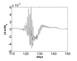
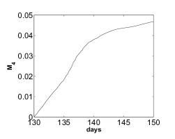
a) b) c)

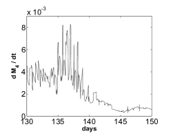
Figure 23: a) Evaluation of the $x$ component of the vector $d{\bf a}/dt$ along a trajectory from $t-\tau$ to $t+\tau$; b) evolution of $M_{4}$ in the same time interval; c) evolution of the time derivative of $M_{4}$.

Despite the lack of regularity displayed in Figure 23a), the actual descriptor is more regular since it is based on integrals over these functions. Figure 23b) shows the evolution versus $\tau$ of $M_{4}$. Figure 23c) displays the time derivative of $M_{4}$, confirming that its regularity is comes from that of $d{\bf a}/dt$. Expression (39) shows that the evaluation of acceleration along trajectories involves first order spatial derivatives of the velocity field (50). Figure 24a) shows the evolution of the horizontal component of acceleration, which confirms that the regularity of the interpolator of the underlying velocity field is observable. The actual regularity of $M_{2}$ is larger than that of acceleration as it is based on integrals over these quantities. Figure 24b) shows the evolution versus $\tau$ of $M_{2}$ as a more regular curve, and in c) the time derivative of $M_{2}$, confirms that its regularity comes from that of ${\bf a}$.

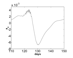
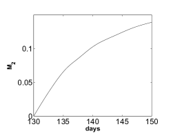
a)b) c)

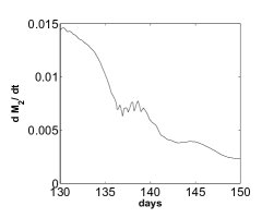
Figure 24: Evaluation of the $x$ component of the vector ${\bf a}$ along a trajectory from $t-\tau$ to $t+\tau$; b) evolution of $M_{2}$ in the same time interval; c) evolution of the time derivative of $M_{2}$.

The performance of FTLE is similar to the performance of Lagrangian descriptors involving the evaluation of acceleration, as they require the evaluation of the gradient of the flow map. The gradient of the flow map is based on integrations on linear equations which are obtained by linearizing the velocity field (50) along a trajectory. This involves evaluating first order spatial derivatives, as in the case of acceleration. Figure 25a) shows the partial derivative of $v_{x}$ with respect to $y$ along the same trajectory as above, for backwards integration. The lack of regularity is noticed, however as the FTLE computation is based on integrations along this linearized field, it gains regularity and for instance in Figure 25b) we show the evolution of one of the components of the matrix $N$ used to compute the FTLE. Again in Figure 25c) illustrates how the regularity of the backwards FTLE is governed by the regularity of linearized velocity fields. Finally we note that descriptors based on the integration of the velocity are the most regular. They are advantageous in this regard not only to those LD involving acceleration or its time derivative, but also to FTLE.

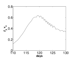
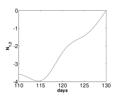
a) b) c)

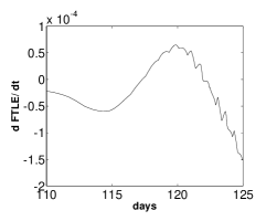
Figure 25: a) Evolution of $\partial_{y}v_{x}({\bf x}(t))$ versus $t$ for backwards intergation; b) evolution of the $N_{1,2}$ component versus $t$ for backwards integration; c) evolution of the time derivative of the backwards FTLE.

The discussed reasons suggest that for analyzing velocities fields given as data sets, the choice of Lagrangian descriptors involving $d{\bf a}/dt$ may be less appropriate than those involving ${\bf v}$ or ${\bf a}$ since they require interpolators with a higher order of regularity than is required by the latter quantities. On the other hand, for data sets interpolated with not too regular interpolators, Lagrangian descriptors based on ${\bf v}$ are the better choice, even with respect to FTLE.

References

- Acar et al. (2012) Acar, E., Senst, T., Kuhn, A., Keller, I., Theisel, H., Albayrak, S., and Sikora, T. (2012). Human action recognition using Lagrangian descriptors. In IEEE Conference Publications, 2012 IEEE 14th International Workshop on Multimedia Signal Processing (MMSP), pages 360–365. IEEE.
- Aref (1984) Aref, H. (1984). Stirring by chaotic advection. J. Fluid Mech., 143, 1–21.
- Balibrea et al. (2010) Balibrea, F., Caraballo, T., Kloeden, P. E., and Valero, J. (2010). Recent developments in dynamical systems: Three perspectives. Int. J. Bif. Chaos, 20(9), 2591–2636.
- Beron-Vera et al. (2010) Beron-Vera, F. J., Olascoaga, M. J., Brown, M. G., Kocak, H., and Rypina, I. I. (2010). Invariant-tori-like Lagrangian coherent structures in geophysical flows. Chaos, 20, 017514.
- Branicki and Wiggins (2009) Branicki, M. and Wiggins, S. (2009). An adaptive method for computing invariant manifolds in non-autonomous, three-dimensional dynamical systems. Physica D, 238(16), 1625 – 1657.
- Branicki and Wiggins (2010) Branicki, M. and Wiggins, S. (2010). Finite-time Lagrangian transport analysis: stable and unstable manifolds of hyperbolic trajectories and finite-time Lyapunov exponents. Nonlin. Proc. Geophys., 17, 1–36.
- Branicki et al. (2011) Branicki, M., Mancho, A. M., and Wiggins, S. (2011). A Lagrangian description of transport associated with a front-eddy interaction: application to data from the North-Western Mediterranean sea. Physica D, 240(3), 282–304.
- Cabral and Leedom (1993) Cabral, B. and Leedom, L. (1993). Imaging vector fields using line integral convolution. In Proc. Siggraph, pages 263–270. ACM Press.
- Coppel (1978) Coppel, W. A. (1978). Dichotomies in Stability Theory, volume 629 of Lecture Notes in Mathematics. Springer-Verlag, New York, Heidelberg, Berlin.
- Coulliette and Wiggins (2001) Coulliette, C. and Wiggins, S. (2001). Intergyre transport in a wind-driven, quasigeostrophic double gyre: an application of lobe dynamics. Nonlin. Proc. Geophys., 8, 69–94.
- de la Cámara et al. (2012) de la Cámara, A., Mancho, A. M., Ide, K., Serrano, E., and Mechoso, C. (2012). Routes of transport across the Antarctic polar vortex in the southern spring. J. Atmos. Sci., 69(2), 753–767.
- Dieci and Vleck (2002) Dieci, L. and Vleck, E. S. V. (2002). Lyapunov spectral intervals: Theory and computation. SIAM J. Numer. Anal., 40(2), 516–542.
- Dieci et al. (1997) Dieci, L., Russell, R. D., and Vleck, E. S. V. (1997). On the computation of Lyapunov exponents for continuous dynamical systems. SIAM J. Numer. Anal., 34(1), 402–423.
- Duarte (1999) Duarte, P. (1999). Abundance of elliptic isles at conservative bifurcations. Dyn. Stab. Sys., 14(4), 339–356.
- Duc and Siegmund (2008) Duc, L. H. and Siegmund, S. (2008). Hyperbolicity and invariant manifolds for planar nonautonomous systems on finite time intervals. Int. J. Bif. Chaos, 18(3), 641–674.
- Goldhirsch et al. (1987) Goldhirsch, I., Sulem, P.-L., and Orszag, S. (1987). Stability and Lyapunov stability of dynamical systems: a differential approach and a numerical method. Physica D, 27, 311–337.
- Gonchenko and Silnikov (2000) Gonchenko, S. V. and Silnikov, L. P. (2000). On two dimensional area preserving diffeomorphisms with infinitely many elliptic islands. J. Stat. Phys., 101(1/2), 321–356.
- Haller (2000) Haller, G. (2000). Finding finite-time invariant manifolds in two-dimensional velocity fields. Chaos, 10(1), 99–108.
- Haller (2001) Haller, G. (2001). Lagrangian structures and the rate of strain in a partition of two-dimensional turbulence. Physics of Fluids, 13(11), 3365–3385.
- Huhn et al. (2012) Huhn, F., von Kameke, A., Perez-Munuzuri, V., Olascoaga, M. J., and Beron-Vera, F. J. (2012). The impact of advective transport by the South Indian ocean countercurrent on the Madagascar plankton bloom. Geophys. Res. Lett., 39(6), L06602.
- Ide et al. (2002) Ide, K., Small, D., and Wiggins, S. (2002). Distinguished hyperbolic trajectories in time dependent fluid flows: analytical and computational approach for velocity fields defined as data sets. Nonlin. Proc. Geophys., 9, 237–263.
- Jones and Winkler (2002) Jones, C. K. R. T. and Winkler, S. (2002). Invariant manifolds and Lagrangian dynamics in the ocean and atmosphere. In Handbook of dynamical systems, pages 55–92. North-Holland, Amsterdam.
- Kreyszig (1991) Kreyszig, E. (1991). Differential Geometry. Dover.
- Lapeyre (2002) Lapeyre, G. (2002). Characterization of finite-time Lyapunov exponents and vectors in two-dimensional turbulence. Chaos, 12, 688=698.
- Legras and Vautard (1996) Legras, B. and Vautard, R. (1996). A guide to Liapunov vectors. In T. Palmer, editor, Predictability, volume 1, pages 135–146, Reading, UK. ECMWF.
- Lekien et al. (2007) Lekien, F., Shadden, S., and Marsden, J. E. (2007). Lagrangian coherent structures in n-dimensional systems. J. Math. Phys., 48, 065404.
- Madrid and Mancho (2009) Madrid, J. A. J. and Mancho, A. M. (2009). Distinguished trajectories in time dependent vector fields. Chaos, 19, 013111.
- Malhotra et al. (1998) Malhotra, N., Mezic, I., and Wiggins, S. (1998). Patchiness: A new diagnostic for Lagrangian trajectory analysis in time-dependent fluid flows. Int. J. Bif. Chaos, 8(6), 1053–1093.
- Mancho et al. (2003) Mancho, A. M., Small, D., Wiggins, S., and Ide, K. (2003). Computation of stable and unstable manifolds of hyperbolic trajectories in two-dimensional, aperiodically time-dependent vectors fields. Physica D, 182, 188–222.
- Mancho et al. (2004) Mancho, A. M., Small, D., and Wiggins, S. (2004). Computation of hyperbolic and their stable and unstable manifolds for oceanographic flows represented as data sets. Nonlin. Proc. Geophys., 11, 17–33.
- Mancho et al. (2006a) Mancho, A. M., Small, D., and Wiggins, S. (2006a). A comparison of methods for interpolating chaotic flows from discrete velocity data. Computers and Fluids, 35, 416–428.
- Mancho et al. (2006b) Mancho, A. M., Hernández-García, E., Small, D., Wiggins, S., and Fernández, V. (2006b). Lagrangian transport through an ocean front in the North-Western Mediterranean sea. J. Phys. Oceanogr., 38(6), 1222–1237.
- Mancho et al. (2006c) Mancho, A. M., Small, D., and Wiggins, S. (2006c). A tutorial on dynamical systems concepts applied to Lagrangian transport in oceanic flows defined as finite time data sets: Theoretical and computational issues. Phys. Rep., 237(3-4).
- Mendoza and Mancho (2010) Mendoza, C. and Mancho, A. M. (2010). The hidden geometry of ocean flows. Phys. Rev. Lett., 105(3), 038501.
- Mendoza and Mancho (2012) Mendoza, C. and Mancho, A. M. (2012). The Lagrangian description of ocean flows: a case study of the Kuroshio current. Nonlin. Proc. Geophys., 19(4), 449–472.
- Mendoza et al. (2010) Mendoza, C., Mancho, A. M., and Rio, M.-H. (2010). The turnstile mechanism across the Kuroshio current: analysis of dynamics in altimeter velocity fields. Nonlin. Proc. Geophys., 17(2), 103–111.
- Mezic and Wiggins (1999) Mezic, I. and Wiggins, S. (1999). A method for visualization of invariant sets of dynamical systems based on the ergodic partition. Chaos, 9(1), 213–218.
- Mezic et al. (2010) Mezic, I., Loire, S., Fonoberov, V. A., and Hogan, P. A. (2010). A new mixing diagnostic and Gulf oil spill movement. Science, 330(6003), 486–489.
- Newhouse (1977) Newhouse, S. E. (1977). Quasi-elliptic periodic points in conservative dynamical systems. Amer. J. Math., 99(5), 1061–1087.
- Okubo (1970) Okubo, A. (1970). Horizontal dispersion of floatable trajectories in the vicinity of velocity singularities such as convergencies. Deep Sea Res., 17, 445–454.
- O’Neill et al. (1994) O’Neill, A., Grose, W. L., Pope, V. D., McLean, H., and Swinbank, R. (1994). Evolution of the stratosphere during northern winter 1991-1992 as diagnosed by the UKMO analysis. J. Atmos. Sci., 51, 2800–2817.
- Oseledets (1968) Oseledets, V. I. (1968). A multiplicative ergodic theorem. Lyapunov characteristic numbers for dynamical systems. Trans. Mosc. Math. Soc., 19, 197–231.
- Ottino (1989) Ottino, J. M. (1989). The Kinematics of Mixing: Stretching, Chaos, and Transport. Cambridge University Press, Cambridge, England. Reprinted 2004.
- Poincaré (1890) Poincaré, H. (1890). Sur le problème des trois corps et les équations de la dynamique. Acta Mathematica, 13, 1–270.
- Poje et al. (1999) Poje, A., Haller, G., and Mezic, I. (1999). The geometry and statistics of mixing in aperiodic flows. Phys. Fluids, 11(10), 2963–2968.
- Prants (2013) Prants, S. V. (2013). Dynamical systems theory methods for studying mixing and transport in the ocean. Physica Scripta, 87, 0381115.
- Prants et al. (2011a) Prants, S. V., Budyansky, M., Ponomarev, V. I., and Uleysky, M. Y. (2011a). Lagrangian study of transport and mixing in a mesoscale eddy street. Ocean Modelling, 38(1-2), 114–125.
- Prants et al. (2011b) Prants, S. V., Uleysky, M. Y., and Budyansky, M. V. (2011b). Numerical simulation of propagation of radioactive pollution in the ocean from the Fukushima dai-ichi nuclear power plant. Doklady Earth Science, 439(2), 1179–1182.
- Prants et al. (2013) Prants, S. V., Ponomarev, V. I., Budyansky, M. V., Uleysky, M. Y., and Fayman, P. A. (2013). Lagrangian analysis of mixing and transport of water masses in the marine bays. Izvestiya Atmospheric and Oceanic Physics, 49(1), 82–96.
- Press et al. (1999) Press, W., Teukolsky, S., Vetterling, W., and Flannery, B. (1999). Numerical Recipes in Fortran 77, The Art of Scientific Computing. Cambridge University Press, Cambdridge, 2 edition.
- Rokhlin (1966) Rokhlin, V. A. (1966). Selected topics from the metric theory of dynamical systems. Amer. Math. Soc. Transl. Series 2, 49, 171–240.
- Rowley (1996) Rowley, C. (1996). A Modeling Study of the North Atlantic Current. Ph.D. thesis, University of Rhode Island, Kingston, RI.
- Rypina et al. (2011) Rypina, I. I., Scott, S. E., Pratt, L. J., and Brown, M. G. (2011). Investigating the connection between complexity of isolated trajectories and Lagrangian coherent structures. Nonlin. Proc. Geophys., 18, 977–987.
- Samelson and Wiggins (2006) Samelson, R. and Wiggins, S. (2006). Lagrangian Transport in Geophysical Jets and Waves: The Dynamical Systems Approach. Springer-Verlag, New York.
- Shadden (2005) Shadden, S. C. (2005). Lagrangian coherent structures. Analysis of time-dependent dynamical systems using finite-time Lyapunov exponents. http://mmae.iit.edu/shadden/LCS-tutorial/overview.html/.
- Shadden et al. (2005) Shadden, S. C., Lekien, F., and Marsden, J. E. (2005). Definition and properties of Lagrangian coherent structures from finite-time lyapunov exponents in two-dimensional aperiodic flows. Physica D, 212, 271–304.
- Shi et al. (2008) Shi, K., Theisel, H., Weinkauf, T., Hege, H.-C., and Seidel, H.-P. (2008). Visualizing transport structures of time-dependent flow fields. IEEE Computer Graphics & Applications, pages 24–36.
- Sutton et al. (1994) Sutton, R. T., McLean, H., Swinbank, R., O’Neill, A., and Taylor, F. W. (1994). High resolution stratospheric tracer fields estimated from satellite observations using Lagrangian trajectory calculations. J. Atmos. Sci., 51, 2995–3005.
- Weiss (1991) Weiss, J. (1991). The dynamics of enstrophy transfer in 2-dimensional hydrodynamics. Physica D, 48, 273–294.
- Wiggins (2005) Wiggins, S. (2005). The dynamical systems approach to Lagrangian transport in oceanic flows. Annu. Rev. Fluid Mech., 37, 295–328.
- Wiggins and Ottino (2004) Wiggins, S. and Ottino, J. (2004). Foundations of chaotic mixing. Phil. Trans. Roy. Soc., 362 (1818), 937–970.