Abstract

A theoretical scheme is introduced to generate entangled network via Dzyaloshinskii- Moriya (DM)interaction. The dynamics of entanglement generated between different nodes by direct or indirect interaction is investigated. It is shown that, the direction of (DM) interaction and the location of the nodes have a sensational effect on the degree of entanglement. We quantify the minimum entanglement generated between all the nodes. The upper and lower bound of the entanglement of the generated network depends on the direction of DM interaction and the repetition of the behavior depends on the strength of DM. The generated entangled nodes are used as quantum channel to perform quantum teleportation, where we show that the fidelity of teleporting unknown information between the network members depends on the location of the members.

Keywords:Entanglement, Network, Teleportation.

1 Introduction

Quantum entanglement is considered as a promising resource for quantum information and computation fields[1]. Long surviving generated entangled states is an important issue in the context of quantum information processing[2]. Generating entangled state between different types of bipartite systems have been extensively investigated [3]. Multi-parties entanglement is more powerful than bipartite entanglement in quantum information processing. For example, M. Siomau and et. al. [4] discussed the entanglement evolution of multi-qubit systems when one of its qubits is subjected to a general noisy channel. Multipartite entangled states with two bosonic modes and qubits have been discussed by Munhoz and Semi$\tilde{a}$o [5]. Perseguers and et.al. [6] have studied the problem of creating a long-distance entangled state between two stations of a network. A general scheme for construction of noiseless networks detecting entanglement with the help of linear, hermiticity-preserving maps have been introduced in [7].

In this contribution, we introduce a theoretical technique to generate entangled network by using pairs of maximum entangled states. The description of this scheme is shown in Fig.1, where it is assumed that a source supplies the users with pairs of Bell states. The second and third qubits entangle together via Zyaloshinskii- Moriya (DM) interaction [8]. This type of interaction is very important in the context of quantum information and entanglement, where Chutia and et.al [9] have proposed an experiment using coupled quantum dots to detect and characterize the DM interaction. Also in [10] the Dzyaloshinskii Moriya interaction has been detected by means of pulsed EPR spectroscopy.

Due to this interaction, all the qubits which represent nodes in the network are entangled together(the details are given in Sec.2). We investigated the dynamics of entanglement generated between the different nodes interacting directly or indirectly. The possibility of using these channels to perform quantum teleportation. is discussed

The paper is organized as follows In Sec.2, we introduce the system and its analytical solution. The dynamics of the entanglement between different nodes is investigated in Sec.3.1. The upper and lower bounds of entanglement for the generated entangled network is quantified in Sec.3.2. We introduce an extension to the network to include more nodes in Sec.4. Employing the entangled channel between the different nodes to achieve quantum teleportion is discussed in Sec.5. Finally we summarize our results in Sec.6.

2 The System

Let us assume that we have a source suppling the users with two qubit pairs prepared in one of the Bell (EPR)states, $\bigl{|}\phi^{\pm}\bigr{\rangle}=\frac{1}{\sqrt{2}}(\bigl{|}11\bigr{\rangle}\pm\bigl{|}00\bigr{\rangle}),\bigl{|}\psi^{\pm}\bigr{\rangle}=\frac{1}{\sqrt{2}}(\bigl{|}10\bigr{\rangle}\pm\bigl{|}01\bigr{\rangle})$[11]. For a convenience, these EPR states are described by Pauli matrices. For example, the density operator $\rho_{\phi^{+}}=\bigl{|}\phi^{+}\bigr{\rangle}\bigl{\langle}\phi^{+}\bigr{|}$ takes the following form

$$\rho_{\phi^{+}}=\frac{1}{4}(1+\sigma_{x}\tau_{x}-\sigma_{y}\tau_{y}+\sigma_{z}\tau_{z}),$$ (1)

where, the vectors $\mathord{\buildrel\lower 3.0pt\hbox{$\scriptscriptstyle\rightarrow$}\over{\sigma}_{i}}=(\sigma_{x},\sigma_{y},\sigma_{z})$ and $\mathord{\buildrel\lower 3.0pt\hbox{$\scriptscriptstyle\rightarrow$}\over{\tau}_{j}}=\tau_{x},\tau_{y},\tau_{z})$ are Pauli operators (see for example[12]). Each qubit is sent to two distinct partners, which represent nodes in the network. These nodes are connected together via Dzyaloshinskii- Moriya (DM) interaction, where the end of each entangle node interacts with the first node of the other entangled two nodes. To clarify this suggested network, we start with four nodes network. Therefore, the initial state vector of the network is given by

$$\rho_{1234}(0)=\rho_{\phi^{+}_{12}}\otimes\rho_{\phi^{+}_{34}},$$ (2)

where $\rho_{\phi_{12}^{+}}$ and $\rho_{\phi_{34}^{+}}$,

$$\rho_{\phi_{12}^{+}} = \frac{1}{4}(1+\sigma^{(1)}_{x}\tau^{(2)}_{x}-\sigma^{(1)}_{y}\tau^{(2)}_{y}+\sigma^{(1)}_{z}\tau^{(2)}_{z}),$$

$$\rho_{\phi_{34}^{+}} = \frac{1}{4}(1+\sigma^{(3)}_{x}\tau^{(4)}_{x}-\sigma^{(3)}_{y}\tau^{(4)}_{y}+\sigma^{(3)}_{z}\tau^{(4)}_{z}).$$ (3)

The nodes $2$ and $3$ are connected via DM interaction, which is defined by,

$$H_{DM}=\mathord{\buildrel\lower 3.0pt\hbox{$\scriptscriptstyle\rightarrow$}\over{D}}\cdot(\mathord{\buildrel\lower 3.0pt\hbox{$\scriptscriptstyle\rightarrow$}\over{\sigma}_{i}}\times\mathord{\buildrel\lower 3.0pt\hbox{$\scriptscriptstyle\rightarrow$}\over{\tau}_{j}}).$$ (4)

The components of the vector $\mathord{\buildrel\lower 3.0pt\hbox{$\scriptscriptstyle\rightarrow$}\over{D}}=(D_{x},D_{y},D_{z})$ are the strength of $DM$ interaction in the directions of $x,y$ and $z-$ axis [13]. In this treatment, we consider that DM interaction is switched on the $z-$ or $x-$ axis. The time evolution of the initial network (2) is given by

$$\rho_{1234}(t)=\mathcal{U}_{z}(t)\rho_{1234}(0){\mathcal{U}^{\dagger}_{z}(t)},$$ (5)

where $\mathcal{U}_{z}(t)$ represents the unitary operator when DM interaction is switched on the $z$-axis. In terms of Pauli operators, it takes the form,

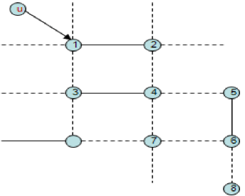
Figure 1: The suggested network consists of a pair of maximum entangled nodes of Bell type which is represented by the solid line as $\rho_{12}$ and $\rho_{34}$. The dot lines represent the generated entangled nodes via direct or indirect interaction. The qubit $u$, is unknown information is given to the node $1$ who wish to teleport to any another node on the network.

$$\mathcal{U}^{(23)}_{z}(t)=cos^{2}(D_{z}t)+\sin^{2}(D_{z}t)\tau^{(2)}_{z}\sigma_{z}^{(3)}-\frac{i}{2}\sin(2D_{z}t)(\tau^{(2)}_{x}\sigma^{(3)}_{y}-\tau^{(2)}_{y}\sigma^{(3)}_{x}),$$ (6)

where we assume that the interaction is running between qubits $2$ and $3$. Since, we are interested in investigating the properties of the channels between the nodes, we calculate the density operator for each subsystem in this network. For example, the density operator between the nodes $1$ and $2$ is given by $\rho_{12z}=tr_{34}\{\rho_{1234z}(t)\}$,

$$\rho_{12z}(t)=\frac{1}{4}(1+c^{(12)}_{xx}\sigma_{x}^{(1)}\tau_{x}^{(2)}-c^{(12)}_{yy}\sigma_{y}^{(1)}\tau_{y}^{(2)}+c^{(12)}_{zz}\sigma_{z}^{(1)}\tau_{z}^{(2)}),$$ (7)

where $c^{(12)}_{xx}=-c^{(12)}_{yy}=\cos^{4}(D_{z}t)-\sin^{4}(D_{z}t)$ and $c^{(12)}_{zz}=\bigl{(}\cos^{4}(D_{z}t)+\sin^{4}(D_{z}t)\bigr{)}-\sin^{2}(2D_{z}t)$. It is clear that the state (7) is no longer maximum entangled state and it is of Werner type [14]. This means that due to the interaction with its neighbor entangled two nodes, the initial state $\rho_{\phi^{+}_{12}}$ loose some of its entanglement. Also, the density operator between the nodes $"1"$ and $"3"$ ($\rho_{13}$) is defined by

$$\rho_{13z}=\frac{1}{4}(1-c^{(13)}_{xy}\sigma^{(1)}_{x}\tau^{(3)}_{y}+c^{(13)}_{yx}\sigma^{(1)}_{y}\tau_{x}^{(3)}+c^{(13)}_{zz}\sigma^{(1)}_{z}\tau^{(3)}_{z}),$$ (8)

where $c^{(13)}_{xy}=c^{(13)}_{yx}=\frac{i}{4}\cos^{2}([D_{z}t)\sin(2D_{z}t),c^{(13)}_{zz}=\frac{1}{2}(1+\frac{1}{2}\sin^{2}(2D_{z}t))$. Similarly, the density operator between the nodes $"1"$ and $"4"$, $\rho_{14z}=tr_{23}\{\rho_{1234z}(t)\}$ is defined by

$$\rho_{14z}(t)=\frac{1}{4}(1+c^{(14)}_{xy}\sigma_{x}^{(1)}\tau^{(4)}_{y}-c^{(14)}_{yx}\sigma^{(1)}_{y}\tau^{(4)}_{x}+c^{(14)}_{zz}\sigma^{(1)}_{z}\tau^{(4)}_{z}),$$ (9)

where $c^{(14)}_{xy}=c^{(14)}_{yx}=i\sin^{2}(2D_{z}t)\cos^{2}D_{z}t,~{}c^{(14)}_{zz}=\frac{1}{2}\bigl{[}1-\cos(2D_{z}t)-4\sin^{2}(2D_{z}t)\bigr{]}.$ The density operator between the systems $2$ and $3$, which represent the direct interaction system is given by

$$\rho_{23z}(t)=\frac{1}{4}(1+c^{(23)}_{xx}\sigma^{(2)}_{x}\tau^{(3)}_{x}+c^{(23)}_{yy}\sigma^{(2)}_{y}\tau^{(3)}_{y}+c^{(23)}_{xy}\sigma_{x}^{(2)}\tau^{(3)}_{x}-c^{(23)}_{yx}\sigma^{(2)}_{y}\tau^{(3)}_{x}+c^{(23)}_{zz}\sigma^{(2)}_{z}\tau^{(3)}_{z}),$$ (10)

where,

$$c^{(23)}_{xx} = c^{(23)}_{yy}=\sin(2D_{z}t)\Bigl{[}\frac{1}{2}\sin^{2}(D_{z}t)-\frac{3}{4}\cos^{2}(D_{z}t)\Bigr{]},$$

$$c^{(23)}_{xy} = c^{(23)}_{yx}=\frac{i}{2}\sin(2D_{z}t)\Bigl{[}1-\frac{1}{2}\cos^{2}(D_{z}t)\Bigr{]},$$

$$c^{(23)}_{zz} = \frac{9}{2}\sin^{2}(2D_{z}t).$$ (11)

The generated entangled channel between the nodes $"2"$ and $"4"$ is defined by

$$\rho_{24z}=\frac{1}{4}(1+c^{(24)}_{zz}\sigma^{(2)}_{z}\tau^{(4)}_{z}),$$ (12)

where $c^{(24)}_{zz}=\frac{1}{2}+\frac{1}{8}\sin(2D_{z}t)^{2}-\frac{1}{2}\cos^{2}(2D_{z}t)$.

Let us consider that the DM interaction is switched on the $x-$ axis. In this case, the unitary operator is described by,

$$\mathcal{U}^{(23)}_{x}(t)=cos^{2}(D_{x}t)+\sin^{2}(D_{x}t)\tau^{(2)}_{x}\sigma_{x}^{(3)}-\frac{i}{2}\sin(2D_{x}t)(\tau^{(2)}_{z}\sigma^{(3)}_{y}-\tau^{(2)}_{y}\sigma^{(3)}_{z}),$$ (13)

where $D_{x}$ represents the strength of the interaction in the $x-$ direction. It is possible to obtain the density operators for all the quantum channels which are generated by the direct or indirect interaction. For example, the entangled quantum channel between the nodes $1$ and $2$, $\rho_{12x}(t)$ evolves as

$$\rho_{12x}=\frac{1}{4}(1+c^{(12)}_{xx}\sigma^{(1)}_{x}\tau^{(2)}_{x}+c^{(12)}_{yy}\sigma^{(2)}_{y}\tau^{(2)}_{y}+c_{zz}^{(12)}\sigma_{z}^{(1)}\tau_{z}^{(2)}),$$ (14)

where $c^{(12x)}_{xx}=1-\frac{3}{2}\sin^{2}(2D_{x}t),~{}c^{(12x)}_{yy}=-\bigl{(}\cos^{4}(D_{x}t)-\sin^{4}(D_{x}t)\bigr{)}$ and $c^{(12x)}_{zz}=-c^{(12x)}_{yy}$. Similarly one obtains the density operators for the other subsystems. As a direct interaction, we consider the density operator between the second and third node, $\rho_{23x}=tr_{14}\{\rho_{1234}\}$ which takes the form,

$$\rho_{23x}=\frac{1}{4}(1+c^{(23x)}_{xx}\sigma^{(2)}_{x}\tau^{(3)}_{x}+c^{(23x)}_{yy}\sigma^{(2)}_{y}\tau^{(3)}_{y}),$$ (15)

where $c^{(23x)}_{xx}=-\frac{1}{2}\sin^{2}(2D_{x}t),~{}c^{(23x)}_{yy}=\frac{5}{4}\sin^{2}(2D_{x}t)$.

3 Network Correlation

3.1 Bi-partite entanglement

In preceding section, we showed that there are some new channels that have been generated due to the indirect interaction. The initial entangled nodes are no longer maximum entangled. In this section, we investigate the entanglement dynamics of the initial entangled nodes and quantify how much of entanglement survive between them. Also, we quantify the amount of entanglement which is generated between the nodes via indirect interaction. The simplest way to do this is to use Wootters concurrence as a measure of the degree of entanglement [15]. A two-qubit entanglement is quantified by the concurrence, whose definition is given by

$$\mathcal{C}=max\bigl{\{}\sqrt{\lambda_{1}}-\sqrt{\lambda_{2}}-\sqrt{\lambda_{3}}-{\sqrt{\lambda}_{4}},0\bigr{\}},$$ (16)

where $\lambda_{1}\geq\lambda_{2}\geq\lambda_{3}\geq\lambda_{4}$ are the square roots of the eigenvalues of $\bar{\rho}\rho$. The density operator $\rho$ represents the reduced density operator of the total system and $\bar{\rho}=\sigma_{y}\tau_{y}\rho^{*}\tau_{y}\sigma_{y}$ with $\rho^{*}$ is the complex conjugate of $\rho$.

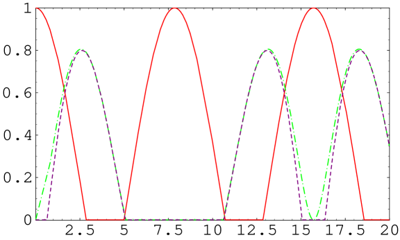
Figure 2: The dynamics of entanglement between different nodes. The solid, dash dot and dot curves represent the dynamics of the concurrence $\mathcal{C}_{ijz},ij=12,13,14$ respectively. The DM interaction is switched on the $z-$axis with strength $D_{z}=0.2$.

In Fig.(2), we plot the dynamics of the concurrence $\mathcal{C}_{ij}$ between the nodes $i$ and $j$ for the entangled channels $\rho_{ijz},ij=12,13,14$. The solid curve represents the dynamics of the concurrence $\mathcal{C}_{12z}$ for the channel $\varrho_{12z}(t)$. It is clear that at $t=0$, the entanglement is maximum i.e., $\mathcal{C}_{12z}=1$, since the initial state of the nodes $"1"$ and $"2"$, $\varrho_{12z}(0)=\rho_{\phi^{+}}$. However as $t$ increases, $\mathcal{C}_{12}$ fluctuates between the maximum value and a minimum value, $\mathcal{C}_{12z}\simeq 0.25$). Due to the interaction between the second and third nodes of the network there are different entangled channels generated between the other nodes. For example, the entanglement which is generated between the node $"1"$ and $"3"$ is quantified by $\mathcal{C}_{13z}$( dash-dot curve). Since at $t=0$, the nodes $"1"$ and $"3"$ are completely separable, hence the degree of entanglement ($\mathcal{C}_{13z})=0$. However, as the interaction is switched on an entangled channel is generated between these nodes. The degree of entanglement increases to reach its maximum value $(\mathcal{C}_{13z}\simeq 0.79)$. For larger time, the concurrence decreases to reach its minimum value ($\mathcal{C}_{13z}=0$). This means that the two nodes become separable while the state $\rho_{12z}$ turns into a maximum entangled state.

Figure 3: The same as Fig.(1) but for the channels $\rho_{ij},ij=34,23,24$ respectively.

Finally the behavior of $\mathcal{C}_{14z}$ which represents the entanglement between the nodes $"1"$ and $"4"$ shows that the entangled channel is not generated as soon as the interaction is switched on. Also, the general behavior of $\mathcal{C}_{14z}$ is almost the same as that depicted for $\mathcal{C}_{13z}$. This shows that with an equal probability one can generate entangled channels between the node $"1"$ and ($"3"$ or $"4"$) with almost the same degree of entanglement. Therefore, it is possible to send information from node $"1"$ to $"3"$ or $"4"$ with the same fidelity.

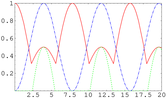
Figure 4: The same as Fig.1 but DM is considered in $x-$ axis with $D_{x}=0.2$.

Fig.(3) displays the dynamics of the concurrence $\mathcal{C}_{ijz}$, $ij=23,24,34$, which measure the entanglement in the channels $\rho_{23z},\rho_{24z},\rho_{34z}$ respectively . The behavior of $\mathcal{C}_{34}$ (solid curve) which represents the entanglement between the nodes $"3"$ and $"4"$, is the same as that shown for the concurrence $\mathcal{C}_{12z}$(solid curve in Fig.1). Also, the dynamics of entanglement between the nodes $"2"$ and $"3"$ is given by the concurrence $\mathcal{C}_{23z}$( dot curve). For $t>0$, $\mathcal{C}_{23z}$ increases smoothly and reaches its upper bound for the first time at $t\simeq 4$. For $t>4$, the entanglement decreases smoothly to vanish completely for the first time at $t\simeq 7.5$. This behavior is repeated depending on the value of the interaction’s strength. At this time all the correlation between the other nodes is almost zero and consequently the network turns into its initial state. As an important observation, the entangled channel between the nodes $"2"$ and $4"$ generated via indirect interaction $\mathcal{C}_{24z}$ is the same as that generated via direct interaction between the nodes $"2"$ and $3"$, namely $\mathcal{C}_{23z}$=$\mathcal{C}_{24z}$ as shown in Fig.(3).

Fig.(4), shows the effect of a different direction of DM interaction, where we assume that it is switched on the $x-$ axis. In this case, the dynamics of entanglement for the initial entangled nodes which is represented by $\mathcal{C}_{12x}$, $\mathcal{C}_{34x}$ for the channels $\rho_{12x}$ and $\rho_{34x}$ respectively are completely different from those displayed in Figs.(2$\&3$). For example, as soon as the interaction is switched on, $\mathcal{C}_{12x}$ decreases smoothly but it doesn’t vanish. Also, the entangled channel between the nodes $"1"$ and $"3"$ turns into maximum entangled channel at $t\simeq 4$ namely $\mathcal{C}_{13x}=1$, while the maximum value of $\mathcal{C}_{13z}\simeq 0.79$. The degree of entanglement between the nodes $"1"$ and $4"$ which is quantified by $\mathcal{C}_{14x}$ is different from the behavior of $\mathcal{C}_{14z}$, where it is generated after a longer time from the beginning of the interaction. The dynamics of entanglement $\mathcal{C}_{23x}$ which is generated between the nodes $2"$ and $"3"$ via a direct interaction is similar to that shown in Fig(3), but its maximum value is smaller than $\mathcal{C}_{23z}$. As a final observation, the dynamics of the entanglement which is generated between the nodes $"2"$ and $"4"$ is the same as that depicted between $"1"$ and $"3"$, namely $\mathcal{C}_{13x}=\mathcal{C}_{24x}$.

From our finding, it is possible to generate entangled channel between the different nodes. The direction of the interaction plays an important role in generating maximum entangled channel.

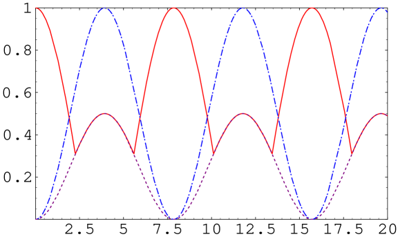
Figure 5: The same as Fig.1 but DM is considered in $x-$ axis with $D_{x}=0.2$.

3.2 Minimum entanglement of the Network

In this subsection, we quantify the minimum amount of entanglement contained in the generated entangled network. We use a measure given by the concurrence introduced in [4, 16]. It states that, for a given pure N-qubit state $\bigl{|}\psi\bigr{\rangle}$, the concurrence is defined by

$$\mathcal{C}_{min}=\sqrt{1-\frac{1}{N}\sum_{i=1}^{N}Tr\rho_{i}^{2}},$$ (17)

where, $\rho_{i}=tr{\bigl{|}\psi\bigr{\rangle}\bigl{\langle}\psi\bigr{|}}$ is the reduced density operator of the i-th qubit which is obtained by tracing out the remaining $N-1$ qubits.

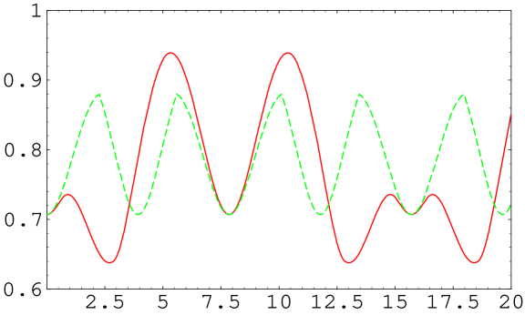
Figure 6: The minimum entanglement of the four qubit network, $\mathcal{C}_{min}$ where DM interaction is switched in the $z-$ axis (solid curve) and in the $x$-axis (dot curve) $D_{z}=D_{x}=0.2$.

Fig.(4), shows the dynamics of the minimum amount of entanglement for the four qubit entangled network, where DM interaction is switched on the $z-$ and $x-$ axis. It is clear that at $t=0$, the concurrence $\mathcal{C}_{min}>0.7$ which represents the lower bound of entanglement. For $t>0$, the dynamics of concurrence depends on the direction of the interaction. It is clear that when DM is switched on the $z-$axis, $\mathcal{C}_{min}$ reaches its minimum value for the first time at $t\simeq 2.6$. On the other hand, if DM is switched on the $x-$axis, the dynamics of $\mathcal{C}_{min}$ is more stable, where it oscillates between a fixed maximum and minimum values.

Therefore, it is possible to generate entangled network by using pairs of EPR interact together via DM interaction. The upper and lower bounds of the entanglement of the generated network depends on the direction DM interaction and the repatation of the behavior depends on the strength of DM interaction.

4 Generalization of the Network

In this section, we extend the entangled network (5) to include more nodes. For this aim, we assume that according to the preceding procedure which is described in Sec.2, there is an entangled network consists of $4$ qubits interact with another two qubit state, $\rho_{56}$ defined as

$$\rho_{\phi_{56}^{+}}=\frac{1}{4}(1+\sigma^{(5)}_{x}\tau^{(6)}_{x}-\sigma^{(5)}_{y}\tau^{(6)}_{y}+\sigma^{(5)}_{z}\tau^{(6)}_{z}).$$ (18)

The time evaluation of the final state is given by,

$$\rho_{1...6}(t)=\mathcal{U}_{45z}(t)\rho(t)_{1..4}\otimes\rho_{\phi^{+}_{56}}\mathcal{U}^{\dagger}_{45z},$$ (19)

where, $\mathcal{U}_{45z}$ represents the unitary operator when DM interaction is switched in the $z-$axis and the interaction is running between the qubits $"4"$ and $5"$.

To show the dynamics of entanglement between different nodes, we have to obtain the reduced density operator of the required subsystem by tracing out the other subsystems. For example, the quantum channel between the nodes $"1"$ and $"5"$ is represented by the density operator $\rho_{15}=tr_{2346}\Bigl{\{}\bigl{|}\psi\bigr{\rangle}_{1...6}\bigl{\langle}\psi\bigr{|}\Bigr{\}}$. In the computational basis one can rewrite this density operator as

$$\rho_{15} = \frac{1}{4}\Bigl{\{}1+(\mu_{1}+\mu_{2}-\mu_{3}-\mu_{4})\sigma_{z}^{(1)}+(\mu_{1}+\mu_{3}-\mu_{2}-\mu_{4})\tau_{z}^{(1)}++i\mu_{5}(\sigma^{(1)}_{x}\tau^{(5)}_{y}-\sigma^{(1)}_{y}\tau^{(5)}_{x})$$ (20)

$$\hskip 170.71652pt+\mu_{6}\sigma_{z}^{(1)}\tau_{x}^{(5)}+(\mu_{1}+\mu_{4}-\mu_{2}-\mu_{3})\sigma^{(1)}_{z}\tau^{(5)}_{z}\Bigr{\}},$$

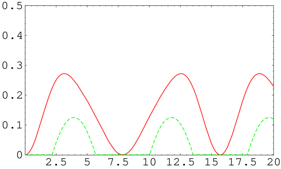
Figure 7: The dynamics of the concurrence $\mathcal{C}_{ij},ij=15,16$ between the nodes $"1"\&"5"$ (solid curve ) and ”$1"\&"6"$(dot curve) where DM interaction is switched in the $z-$ axis,) $D_{z}=D_{x}=0.2$.

where

$$\mu_{1} = \frac{3+\mathcal{S}^{2}}{8},\quad\mu_{2}=\frac{1+\mathcal{S}^{2}}{4},\quad\mu_{3}=\frac{1}{8}\bigl{[}1+\mathcal{S}^{2}(\mathcal{C}^{2}+\mathcal{C})+\mathcal{C}^{2}\bigr{]},$$

$$\mu_{5} = \frac{1}{4}\mathcal{C}\mathcal{S}^{2},\quad\quad\mu_{6}=\frac{1}{4}\bigl{[}\mathcal{S}^{2}(1+\mathcal{C}^{2})+\mathcal{C}^{4}\bigr{]},$$ (21)

In a similar way the density operator between the nodes $"1"$ and $"6"$ is given by

$$\rho_{16} = \frac{1}{4}\Bigl{\{}1+(\nu_{1}+\nu_{4}-\nu_{2}-\nu_{3})\sigma_{z}^{(1)}+(\nu_{1}+\nu_{3}-\nu_{2}-\nu_{4})\tau_{z}^{(1)}+\nu_{5}(\sigma^{(1)}_{x}\tau^{(5)}_{x}-\sigma^{(1)}_{y}\tau^{(5)}_{y})$$ (22)

$$\hskip 113.81102pt+(\nu_{1}+\nu_{2}-\nu_{3}-\nu_{4})\sigma^{(1)}_{z}\tau^{(5)}_{z}\Bigr{\}},$$

where

$$\nu_{1} = \frac{1+\mathcal{S}^{2}}{4},\quad\nu_{2}=\frac{1}{8},\quad\nu_{3}=\frac{1}{8}\bigl{[}2\mathcal{C}^{2}+\mathcal{S}^{2}(1+\mathcal{C}^{2}\bigr{]},$$

$$\nu_{4} = \frac{1}{8}\bigl{[}4+\mathcal{S}^{2}+\mathcal{S}^{4}\bigr{]},\quad\nu_{5}=\frac{1}{8}\mathcal{C}^{2}\mathcal{S}^{2},$$ (23)

where $\mathcal{S}=\sin(2D_{z}t),\mathcal{C}=\cos(2D_{z}t)$.

Fig.7, shows the dynamics of the concurrence for the quantum entangled channels which are generated between the nodes $"1"\&"5"(\rho_{15})$ and $"1"\&"6"(\rho_{16})$. In general the degree of entanglement is much smaller than that depicted Sec.3. The location of the node in the network has a noticeable effect on the entanglement value, where for nearer nodes the entanglement is much larger than that displayed for the long distance locations. Also, the smooth behavior of entanglement is clear for the nearer nodes, while the phenomena of the sudden death and birth is depicted for entanglement which is generated between long distance nodes.

5 Teleportation

In this section, we investigate the possibility of using the generated entangled states between different nodes to communicate among themselves. For this aim we assume that the node $"1"$ is given unknown state defined by $\bigl{|}\psi\bigr{\rangle}_{u}=\alpha\bigl{|}0\bigr{\rangle}+\beta\bigl{|}1\bigr{\rangle}$. The density operator of the state is given by,

$$\rho_{u}=\frac{1}{2}(1+s_{u_{x}}\sigma_{x}+s_{u_{y}}\sigma_{y}+s_{u_{z}}),$$ (24)

where $s_{u_{x}}=\alpha\beta^{*}+\alpha^{*}\beta,s_{u_{y}}=i(\alpha^{*}\beta-\alpha\beta^{*})$ and $s_{u_{z}}=|\alpha|^{2}-|\beta|^{2}$. Then the total state of the network is $\rho_{s}=\rho_{u}\otimes\rho_{ij}$ where $ij=12,13,14$. Now to teleport this state to the nodes $2$, $3$ or $4$, theses nodes perform the following steps [17]:

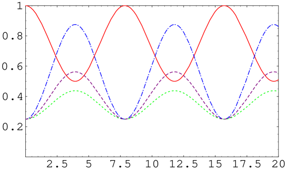
Figure 8: The fidelity of the teleported state from between different channels in the netork.The solid curve represents fidelity of telepoted state from the node 1 to the node $2$ via the channel $\rho_{12}$. The dash-dot curve represents $\mathcal{F}$ via the channel $\rho_{14}$. Finally the dot curve represents the $\mathcal{F}$ via the channel $\rho_{23}$, where DM interaction is considered in the $x$-direction.

1. The first node performs the CNOT operation between its own qubit and the qubit which is located at nodes $2,3$ or $4$.

2. The first node applies the Hadamard on its own particle.

3. Then the first node’s qubit and one of the other qubits are measured randomly in one of the Bell states $\rho_{\phi^{\pm}}$ or $\rho_{\psi^{\pm}}$. Then the teleported state takes the form,

   $$\rho_{t}=\frac{1}{2}(1+s_{t_{x}}\sigma_{x}+s_{t_{y}}\sigma_{y}+s_{t_{z}}\sigma_{z}),$$ (25)

   where $s_{t_{x}},s_{t_{y}},s_{t_{z}}$ are the Bloch vector for the final teleported state. To quantify the closeness of the input state (24) with the final state (25), we evaluate the fidelity $\mathcal{F}$ which is defined as,

   $$\mathcal{F}=\frac{1}{4}(1+s_{u_{x}}s_{t_{x}}+s_{u_{y}x}s_{t_{y}}+s_{u_{z}}s_{t_{z}}).$$ (26)

In Fig.(8), we plot the Fidelity of the teleported state from the node $1$ to the node $2$. It is clear that at $t=0$, the fidelity is maximum $(\mathcal{F}=1$). As soon as the interaction is going on, the fidelity decreases to reach its minimum value ($=0.45)$ at $t\simeq 2.6$. Then the $\mathcal{F}$ re-increases to become maximum at $\simeq 5$. This behavior is repeated periodically depending on the value of the interaction strength, where as $D_{x}$ increases the number of repletion increases. The fidelity of teleportating the unknown state to the node $3$ is defined by the dot curve in Fig.(8). At $t=0$, the fidelity is very small due to the classical correlation and it is called classical teleportation. For $t>0$, there is an entangled state generated between the nodes $2$ and $3$ and hence the fidelity increases to reach its maximum value at $t\simeq 2.6$. However for larger $t$, the fidelity decreases( due to the loss of entanglement between the two nodes) and reaches its minimum value at $t=5$. The same behavior is seen for the fidelity of the teleported state between the nodes $1$ and $4$ (dash-dot curve). It shows that the behavior is the same as that depicted between the nodes (2$\&$ 3), but the maximum values are smaller.

6 conclusion

In this contribution, an entangled network is constructed by using maximum entangled pairs. These pairs, which represent the nodes of the network, interact together via DM interaction, where we consider that DM interaction is switch on the $z-$ or $x-$ directions. Due to this interaction, there are entangled channels generated between these nodes. The amount of entanglement which is contained in these channels is quantified by using Wootters concurrence. It is shown that the phenomena of the sudden death and re-birth of entanglement appear for these channels which are generated via indirect interaction. However, the concurrence increases and deceases smoothly for those channels which are generated via direct interaction. The strength of DM interaction plays an important role on the period of death - rebirth entanglement. Also, for nearer nodes the entangled channels are generated much faster than those located in a long distance.

The amount of entanglement between different channels depends on the direction of DM interaction. We show that when DM is switched on the $x$ axis, there are maximum entangled channels are generated between some nodes and the entanglement of initial entangled nodes doesn’t vanish. However if DM interaction is switched in the $z-$ axis, there is no maximum entangled states between any two nodes generated via indirect interaction while the initial entangled channels loose their entanglement very fast. The minimum amount of entanglement contained in the four-nodes network is quantified. The upper and lower bounds of the entanglement of the generated network depends on the direction of DM interaction and the repatation of the behavior depends on the strength of DM.

Finally, the quantum entangled channels between the different nodes are used to perform quantum teleportation. We clarify this idea by considering the entangled channels generated between different nodes when DM interaction is switched on the $x-$axis. It is clear that the fidelity of the teleported state depends on the location between the nodes. For those initially entangled, the fidelity decreases smoothly but doesn’t vanishe.

References

- [1] M. Neilsen and I. Chaung” quantum computation and Quantum Information( cambridge Univeersity press: New York)” (2000).
- [2] M. Khasin and R. Kosloff, Phys. Rev. A 76 012304 (2007).
- [3] S.-B. Zheng et al., Phys.Rev.Lett. 85 2392 (2000); B. Julsgaard, A. Kozhekin, and E. S. Polzik, Nature 413, 400 (2001); S. Osnaghi et al., Rev. Lett. 87, 037902 (2001); W. Cui, Z. Xi, Y. Pan, J. Phys. A: Math. Theor. 42 155303 (2009); F. Altintas and R. Eryigit, J. Phys. A: Math. Theor.43 415306 (2010).
- [4] M. Siomau and S.Fritzsche, Phys. Rev. A 82, 062327 (2010).
- [5] P. Munhoz, F. L. Semio, Eur. Phys. J. D 59, 509 (2010).
- [6] S. Perseguers, L. Jiang, N. Schuch, F. Verstraete, M.D. Lukin, J.I. Cirac, and K. Vollbrecht, Phys. Rev. A 78, 062324 (2008).
- [7] P. Horodecki, R. Augusiak and M. Demianowicz, Phys. Rev. A 74, 052323 (2006).
- [8] T. Moriya, Phys. Rev. Lett. 4, 228 (1960).
- [9] S. Chutia, M. Friesen, and R. Joynt,Phys. Rev. B bf 73, 241304(R) (2006).
- [10] T. Joutsuka and Y. Tanimura, Chemical Physics Letters 457 237 (2008).
- [11] A. Einstein, B. Podolsky, and N. Rosen, Phys. Rev. 47, 777 (1935); J. Bell, Physics 1, 195 (1964).
- [12] N. Metwally, Int. J. Theor. Phys. 49 1571 (2010).
- [13] X. Wang, Phys. Lett. A 281, 101 (2001); Kheirandish, S. J. Akhtarshenas, and H. Mohammadi, Phys. Rev. A 77, 042309 (2008); F. Kheirandish, S. J. Akhtarshenas, and H. Mohammadi, Eur. Phys. J. D 57, 1 (2010).
- [14] R.F. Werner, Phys. Rev. A 40, 4277 (1989); B. G.-Englert and N. Metwally, ”Kinematics of qubit pairs”, in ”Mathematics of quan- tum computation” by R. Brylinski, G. Chen, Boca Raton pp 25-75(2002).
- [15] W. K. Wootters, Phys. Rev. Lett. 80, 2245 (1998).
- [16] M. Li, S.-M. Fei and Z.-X. Wang, j. Phys. A 42 145303 (2009).
- [17] C.H. Bennett, G. Brassard, C. Cr epeau, R. Jozsa, A. Peres and W.K.Wootters, Phys. Rev. Lett. 70, 1895 (1993).