Computing the Reveals Relation in Occurrence Nets

Abstract

Petri net unfoldings are a useful tool to tackle state-space explosion in verification and related tasks. Moreover, their structure allows to access directly the relations of causal precedence, concurrency, and conflict between events. Here, we explore the data structure further, to determine the following relation: event $a$ is said to reveal event $b$ iff the occurrence of a implies that b inevitably occurs, too, be it before, after, or concurrently with $a$. Knowledge of reveals facilitates in particular the analysis of partially observable systems, in the context of diagnosis, testing, or verification; it can also be used to generate more concise representations of behaviours via abstractions. The reveals relation was previously introduced in the context of fault diagnosis, where it was shown that the reveals relation was decidable: for a given pair $a,b$ in the unfolding $U$ of a safe Petri net $N$, a finite prefix $P$ of $U$ is sufficient to decide whether or not $a$ reveals $b$. In this paper, we first considerably improve the bound on $|P|$. We then show that there exists an efficient algorithm for computing the relation on a given prefix. We have implemented the algorithm and report on experiments.

Topics:

Structure and behaviour of Petri Nets; partial-order theory of concurrency; automatic analysis

1 Introduction

Petri nets (see e.g. [16, 15]) and their partial-order unfoldings [14, 5, 13] have long been used in model checking. Their crucial feature is the partial-order representation of concurrency, allowing to escape from the state-space-explosion problem that is brought about by the use of interleaving semantics [6].

In this paper, we will focus on the problem of determining the following relation: an event $a$ is said to reveal another event $b$ iff, whenever $a$ occurs, the occurrence of $b$ is inevitable. This does not imply that $a$ and $b$ are causally related (though they may be); in fact, $b$ may have occurred before $a$, lie in the future of $a$, or even be concurrent to $a$. To some degree, this relation is complementary to the well-known conflict relation: $a$ and $b$ are in conflict if the occurrence of $a$ implies that the occurrence of $b$ is impossible. Notice however that the conflict relation is symmetric while reveals is not.

We further emphasize that the reveals relation is essentially a non-temporal relation, as opposed to temporal properties or the synchronic distance of e.g. [8, 17, 19]. The latter measures the quantitative degree of independency in the repeated occurrences of two net transitions, whereas $a\mathbin{\triangleright}b$ holds if and only if event $a$ implies event $b$.

The reveals relation was first introduced in [10]; more properties and discussions of its applications are given in [12]. An important motivation for studying reveals lies in the partial observability of many systems in applications such as those related to fault diagnosis. The idea is that $a\mathbin{\triangleright}b$ implies that it suffices to observe $a$ to infer occurrence of $b$; conversely, $b$ does not have to be observable itself, provided $a$ or any other event that reveals $b$ is observable.

This binary relation is the topic of the present article. Recently, [2] gave generalizations that include a reveals relation connecting pairs of sets of events; however, even in this general setting the binary relation turns out to play a central role. Its exploration and effective computation remains therefore an important task, not only for the structural theory. In fact, $\mathbin{\triangleright}$ is relevant in general for opacity-related properties and tasks concerning concurrent systems; potential and actual applications include verification diagnosability (see [12, 11]) and other properties, conformance testing, synthesis of controllers and adaptors.

Concerning the task at hand, note that it was shown in [12] that the reveals relation can be effectively computed for unfoldings of safe nets. For each pair of events $(a,b)$, a suitable finite prefix whose height exceeds that of $a$ and $b$ by at most a uniform bound, is sufficient to verify if $a$ reveals $b$. Here, we make the following contributions:

• We considerably improve the bound on the size of the finite prefix needed to decide whether $a$ reveals $b$. While the previous bound seemed to make this decision impracticable, the new bound gives much more hope to determine the relation in practice.

• Motivated by this, we discuss an efficient algorithm that computes the entire reveals relation within a given prefix. The algorithm can be implemented completely with bitset operations.

• We have implemented the algorithm and report on experiments, notably on the following questions: how big is the prefix necessary to determine the reveals relation, and how much time does it take to compute said relation on a given prefix? Concerning the second question, the algorithm turns out to be suitably fast; it works on prefixes with tens of thousands of events in a few seconds, and usually takes less time than the actual construction of the prefix.

We proceed as follows: Section 2 introduces Petri nets, their unfoldings, the reveals relation, and some of its salient properties. Section 3 gives the new bound on the size of the prefix. Section 4 presents an algorithm for computing reveals on a given prefix, and Section 5 presents the experiments. We conclude in Section 6.

2 Definitions

This section introduces central definitions and facts about Petri nets, their unfoldings, and the reveals relation. While most definitions and some results would be valid in the case of Petri nets that are bounded, but not 1-bounded, our main interest is in 1-bounded (aka safe) nets. Moreover, lifting to non-safe nets brings little additional insight but makes arguments much more technical and cumbersome; we therefore chose to focus on safe nets.

2.1 Petri nets

A Petri net is a triple ${{\mathit{N}}=(P,T,F,M_{0})}$, where $P$ and $T$ are disjoint sets of places and transitions, respectively, and $F\subseteq(P\times T)\cup(T\times P)$ is the flow relation. Any function $M\colon P\to\makebox[1.00006pt][l]{$\mathsf{I}$}\makebox[1.00006pt][l]{$\mathbf{N}$}\hskip 4.49997pt\$ is called a marking, and $M_{0}$ is the initial marking. By node, we shall mean an element from the set $P\cup T$.

In figures (e.g., the left-hand side of Figure 1), circles represent places, rectangular boxes represent transitions, and directed edges represent $F$. A marking $M$ is represented by black tokens.

For a node $x$, call ${{}^{\bullet}{x}}:=\{\,x^{\prime}\mid(x^{\prime},x)\in F\,\}$ the preset, and ${x}^{\bullet}:=\{\,x^{\prime}\mid(x,x^{\prime})\in F\,\}$ the postset of $x$. Moreover, for any set $X\subseteq P\cup T$, set

$${{}^{\bullet}{X}}:=\bigcup_{x\in X}{{}^{\bullet}{x}} and {X}^{\bullet}:=\bigcup_{x\in X}{x}^{\bullet}.$$

Transitions induce a firing relation among markings, as follows: Let $M,M^{\prime}$ be markings and $t$ a transition. Then we write $M\stackrel{{\scriptstyle t}}{{\longrightarrow}}M^{\prime}$ iff $M(p)\geq 1$ for every $p\in{{}^{\bullet}{t}}$ and $M^{\prime}(p)=M(p)-1$ if $p\in{{}^{\bullet}{t}}\setminus{t}^{\bullet}$, $M^{\prime}(p)=M(p)+1$ if $p\in{t}^{\bullet}\setminus{{}^{\bullet}{t}}$, and $M^{\prime}(p)=M(p)$ otherwise. In words, we also say that $t$ is enabled in $M$, and that firing it leads to $M^{\prime}$.

A finite sequence $\sigma:=t_{1}\ldots t_{k}$ of transitions is a run iff $M_{0}\stackrel{{\scriptstyle t_{1}}}{{\longrightarrow}}M_{1}\cdots\stackrel{{\scriptstyle t_{k}}}{{\longrightarrow}}M_{k}$ for some markings $M_{1},\ldots,M_{k}$; if such a run exists, then $M_{k}$ is said to be reachable. The set of reachable markings is denoted $\mathbf{R}(N)$. A net is said to be safe if no reachable marking puts more than one token into any place. As explained above, all the nets we are interested in will be safe. Thus, we shall henceforth treat markings as subsets of $P$.

An infinite sequence $t_{1}t_{2}\ldots$ is called a run if every prefix of it is one. We say that a run $\sigma$ is fair iff

• either $\sigma$ is finite, and in the marking reached by $\sigma$, no transition is enabled;

• or $\sigma=t_{1}t_{2}\ldots$ is infinite, where $M_{1},M_{2},\ldots$ are the markings generated by firing $\sigma$, and there exists no pair $t\in T$ and $i\geq 1$ such that $t$ is enabled in all $M_{k}$,  $k\geq i$ and $t\neq t_{k}$ for all $k>i$.

In other words, a fair run cannot delay firing an enabled transition forever.

2.2 Occurrence nets

Occurrence nets are a specific type of acyclic Petri net. Keeping with tradition, we shall call the places of an occurrence net conditions and its transitions events. Fix a safe Petri net $O=(C,E,F,C_{0})$ for the rest of this subsection. We let $<$ denote the transitive closure of $\mathit{F}$ and $\leq$ the reflexive closure of $<$; further, if $e\in E$ is an event, let $\lceil{e}\rceil:=\{\,e^{\prime}\in E\mid e^{\prime}\leq e\,\}$ be the cone of $e$, and $\lfloor{e}\rfloor:=\lceil{e}\rceil\setminus\{e\}$ the pre-cone of $e$.

Two nodes $x,x^{\prime}$ are in conflict, written $x\mathbin{\#}x^{\prime}$ if there exist $e,e^{\prime}\in E$ such that (i) $e\neq e^{\prime}$, (ii) ${{}^{\bullet}{e}}\cap{{}^{\bullet}{e^{\prime}}}\neq\emptyset$, and (iii) $e\leq x$ and $e^{\prime}\leq x^{\prime}$.

$O$ is called an occurrence net if it satisfies the following properties:

1. no self-conflict: $\forall x\in C\cup E\colon\neg(x\mathbin{\#}x)$;

2. $<$ is acyclic, i.e. $\leq$ is a partial order;

3. finite cones: all events $e$ satisfy $|\lceil{e}\rceil|<\infty$;

4. no backward branching: all conditions $c$ satisfy $|{{}^{\bullet}{c}}|\leq 1$;

5. $C_{0}\subseteq C$ is the set of $\leq$-minimal nodes.

Example 1

The right hand side of Figure 1 shows an occurrence net. The events $a$ and $c$ are both in conflict with $b$, yet not with one another; in fact, they are concurrent (neither ordered nor in conflict).

Figure 1: A Petri net (left) and a prefix of its unfolding (right)

Let $O=(C,E,F,C_{0})$ be an occurrence net. We call $O^{\prime}=(C^{\prime},E^{\prime},F^{\prime},C_{0})$ a prefix of $O$ if

• $C^{\prime}\subseteq C$,  $E^{\prime}\subseteq E$,  $F^{\prime}=F\cap(C^{\prime}\cup E^{\prime})^{2}$, and moreover $C^{\prime}\supseteq C_{0}\cup{(E^{\prime})}^{\bullet}$;

• $C^{\prime}$ and $E^{\prime}$ are downward-closed, i.e. for any $x\in C^{\prime}\cup E^{\prime}$ and $y<x$ we have $y\in C^{\prime}\cup E^{\prime}$.

A prefix is called finite if $C^{\prime}$ and $E^{\prime}$ are finite sets. Notice that each prefix is uniquely determined by its set of events. We denote by $O[E^{\prime}]$ the unique prefix of $O$ whose set of events is $E^{\prime}$.

Let $\mathcal{C}\subseteq E$ be a downward-closed and conflict-free set of events, that is, $e\in\mathcal{C}$ and $e^{\prime}<e$ imply $e^{\prime}\in\mathcal{C}$, and $e,e^{\prime}\in\mathcal{C}$ implies $\neg(e\mathbin{\#}e^{\prime})$. Then we call $\mathcal{C}$ a configuration of $O$. Given a configuration $\mathcal{C}$, we define $\mathit{Cut}(\mathcal{C})$ to be the set of $\leq$-maximal conditions of $O[\mathcal{C}]$. Moreover we define the postfix $O/_{\mathcal{C}}$ to be the occurrence net $(C^{\prime\prime},E^{\prime\prime},F^{\prime\prime},C_{0}^{\prime\prime})$, where $C^{\prime\prime}=C\setminus{{}^{\bullet}{\mathcal{C}}}$,  $E^{\prime\prime}=E\setminus\mathcal{C}$, $F^{\prime\prime}=F\cap(C^{\prime\prime}\cup E^{\prime\prime})^{2}$, and $C_{0}^{\prime\prime}=\mathit{Cut}(\mathcal{C})$.

If $\mathcal{C}$ is a finite configuration and $e\in E\setminus\mathcal{C}$ an event such that ${{}^{\bullet}{e}}\subseteq\mathit{Cut}(\mathcal{C})$. In this case, $\mathcal{C}^{\prime}:=\mathcal{C}\cup\{e\}$ is a configuration, and we write $\mathcal{C}\stackrel{{\scriptstyle e}}{{\leadsto}}$ or $\mathcal{C}\stackrel{{\scriptstyle e}}{{\leadsto}}\mathcal{C}^{\prime}$. By extension, for a finite configuration $\mathcal{C}$ and a set $A=\{e_{1},\ldots,e_{n}\}$ of events, we write $\mathcal{C}\stackrel{{\scriptstyle A}}{{\leadsto}}\mathcal{C}^{\prime}$ iff there exist $\mathcal{C}_{0},\ldots,\mathcal{C}_{n}$ such that $\mathcal{C}_{0}=\mathcal{C}$,  $\mathcal{C}_{n}=\mathcal{C}^{\prime}$, and for all $i=1,\ldots,n$, $\mathcal{C}_{i-1}\stackrel{{\scriptstyle e_{i}}}{{\leadsto}}\mathcal{C}_{i}$. We write $\mathcal{C}\sqsubseteq\mathcal{C}^{\prime}$ if there exists a set $A$ such that $\mathcal{C}\stackrel{{\scriptstyle A}}{{\leadsto}}\mathcal{C}^{\prime}$.

The following facts are well-known, see e.g. [4, 5]:

• A downward-closed set $\mathcal{C}\subseteq E$ is a configuration iff the elements of $\mathcal{C}$ can be arranged to form a run $\sigma$ of $O$. We have that $\sigma$ is fair iff $\mathcal{C}$ is maximal. Moreover, if $\mathcal{C}$ is finite, then $\sigma$ leads from $C_{0}$ to $\mathit{Cut}(\mathcal{C})$.

• For every event $e$, $\lceil{e}\rceil$ and $\lfloor{e}\rfloor$ are configurations.

• Let $c,c^{\prime}\in C$ be a pair of conditions. Then exactly one of the following three statements holds:

  • $c$ and $c^{\prime}$ are causally related, i.e. $c<c^{\prime}$ or $c^{\prime}<c$;

  • $c$ and $c^{\prime}$ are in conflict, i.e. $c\mathbin{\#}c^{\prime}$;

  • $c$ and $c^{\prime}$ are called concurrent, written $c\mathbin{\mathbf{co}}c^{\prime}$, i.e. there exists a configuration $\mathcal{C}$ such that $\{c,c^{\prime}\}\subseteq\mathit{Cut}(\mathcal{C})$.

  A set of pairwise concurrent places is called a co-set.

2.3 Unfoldings

Let ${N=(P,T,F,M_{0})}$ be a safe Petri net. Intuitively, an unfolding of $N$ is an acyclic version of $N$ where loops of $N$ are “unrolled”; an unfolding is usually infinite even if $N$ is finite.

Formally, $U=(C,E,G,C_{0})$ is called an unfolding of $N$ if $U$ is an occurrence net equipped with a mapping $f\colon(C\cup E)\to(P\cup T)$, which we extend to sets and sequences in the usual way. We shall write $f\colon A\leftrightarrow B$ if the restriction of $f$ to $A$ yields a bijection between $A$ and $B$. Then $U$ is the unfolding of $N$ if the following properties hold:

• $f(C)\subseteq P$,  $f(E)\subseteq T$, and $f\colon C_{0}\leftrightarrow M_{0}$;

• for every co-set $D\subseteq C$ and transition $t\in T$ such that $f\colon D\leftrightarrow{{}^{\bullet}{t}}$, there is exactly one event $e\in E$ with $f(e)=t$ and ${{}^{\bullet}{e}}=D$;

• if $f(e)=t$ for some event $e$, then $f\colon{{}^{\bullet}{e}}\leftrightarrow{{}^{\bullet}{t}}$ and $f\colon{e}^{\bullet}\leftrightarrow{t}^{\bullet}$.

With every configuration $\mathcal{C}$ of $U$ we associate the marking $\mathit{Mark}(\mathcal{C}):=\{\,f(c)\mid c\in\mathit{Cut}(\mathcal{C})\,\}$.

Example 2

Figure 1 shows a net $N$ on the left and prefix of its unfolding on the right; the function $f$ is reflected in the inscriptions. It is well-known [4, 5] that $M$ is a reachable marking in $N$ iff there exists a configuration $\mathcal{C}$ of $U$ such that $\mathit{Mark}(\mathcal{C})=M$. Moreover, if $\sigma$ is a run corresponding to $\mathcal{C}$, then $f(\sigma)$ leads from $M_{0}$ to $M$ in $N$. It is in this sense that $U$ mimics the behaviour of $N$.

A prefix $U^{\prime}$ of $U$ is called complete if it “contains” every marking of $N$, i.e. for every reachable marking $M\in\mathbf{R}(N)$ there exists a configuration $\mathcal{C}$ of $U^{\prime}$ such that $\mathit{Mark}(\mathcal{C})=M$. It is well-known that for any configuration $\mathcal{C}$, the postfix $U/_{\mathcal{C}}$ is isomorphic to the unfolding of the net $(P,T,F,\mathit{Mark}(\mathcal{C}))$.

2.4 The “reveals” relation

To illustrate “reveals” we shall study the occurrence net in Figure 2. We are interested in finding relations between events of the form ’if $x$ occurs, then $y$ has already occurred, or will occur eventually’, in the sense that any fair run that contains $x$ also contains $y$. In other words, this means that $y$ is inevitable given $x$.

In the context of Figure 2, it is obvious that, for any fair run $\sigma$,

$$k\in\sigma\Longrightarrow e\in\sigma\Longrightarrow b\in\sigma,$$

where we use $k\in\sigma$ etc informally to mean that $k$ occurs somewhere in $\sigma$. In fact, the statement above simply reflects the causal relationship; if $k$ happens, then surely its cause $e$ must have happened before.

But one also obtains the following facts in Figure 2, again for fair runs $\sigma$:

$$a\in\sigma\iff\neg(b\in\sigma)\iff c\in\sigma\qquad\hbox{and}\qquad c\in\sigma\iff g\in\sigma.$$

Figure 2: Example of an occurrence net

In fact, $a,c$ are a pair of independent transitions which can happen concurrently, where as $c$ is a causal predecessor of $g$ and yet allows to determine that $g$ will eventually happen. The reader is invited to check that these relations follow from the fairness of runs. We thus define our desired relation as follows:

Definition 1

Let $O$ be an occurrence net and $e,e^{\prime}$ be two of its events. We say that $e$ reveals $e^{\prime}$, written $e\mathbin{\triangleright}e^{\prime}$, iff for all fair runs $\sigma$ of $O$ $e\in\sigma$ implies $e^{\prime}\in\sigma$. The revealed range of event $e$ is $\mathord{\mathbin{\triangleright}}[e]:=\{\,e^{\prime}\mid e\mathbin{\triangleright}e^{\prime}\,\}$.

Notice that the definition immediately implies that $\mathbin{\triangleright}$ is reflexive and transitive. Moreover, there is a reveals relationship along causal successors, i.e. if $a<b$, then $b\mathbin{\triangleright}a$. The relation $\mathbin{\triangleright}$ is not symmetric in general: in fact, in Figure 2 we have $h\mathbin{\triangleright}e$ but $\neg(e\mathbin{\triangleright}h)$. On the other hand, $\mathbin{\triangleright}$ is not a partial order: consider $e\mathbin{\triangleright}f$ and $f\mathbin{\triangleright}e$ in Figure 2.

These examples show that the inheritance of conflict along causality relations is not sufficient to derive the statements above. One might therefore suspect that, to obtain the above facts one would have to explore the entire set of configurations. However, the following is known:

Lemma 1 ([10, 12])

For an event $e$, its conflict set is defined as $\#[e]:=\{\,e^{\prime}\mid e\mathbin{\#}e^{\prime}\,\}$. We have that $e\mathbin{\triangleright}e^{\prime}$ iff $\#[e]\supseteq\#[e^{\prime}]$.

Thus, in principle all it takes to see if $e\mathbin{\triangleright}e^{\prime}$ holds is to check whether no witness against it exists for $(e,e^{\prime})$; we call $g$ a witness for the tuple $(e,e^{\prime})$ if $\neg(e\mathbin{\#}g)$ and $e^{\prime}\mathbin{\#}g$. However, notice that this does not provide us with an effective procedure because the conflict sets can be infinite in general (see [12]). In Section 3 we shall show that $e\mathbin{\triangleright}e^{\prime}$ can effectively be decided.

Facets.

Let us just note in passing that the strongly connected components of $\mathbin{\triangleright}$, called facets in [12], form equivalence class of occurrence in the sense that any run $\omega$ that contains any event of a facet must contain all of its events. In Figure 3, the decomposition of the occurrence net from Figure 2 into its facets is shown. The facets are $\{a,d,c,g\},\ \{b,e,f\},\ \{h\},\ \{k\}$; the right hand side shows the occurrence net obtained by abstracting every facet into a single event. In general, quotienting an occurrence net into its facets and their boundary conditions yields an occurrence net whose set of maximal runs is in bijection with that of the initial occurrence net; this procedure (for details see [12]) can reduce the model size for analyses of any properties regarding maximal behaviours. In [2], we focus on reduced nets, i.e. where the contraction of facets has been carried out, and every event is a facet; in this framework, behavioural properties can be specified in a dedicated logic ERL, for which the synthesis problem is solved in [2]; the occurrence nets obtained in a canonical way from a logical formula belong to a distinguished subclass of reduced occurrence nets, the tight nets. For more traditional applications, the facet decomposition can in general yield fast sufficient criteria for verifying properties. Consider observability-related properties Petri nets (see [10, 11] for a detailed discussion on diagnosability): if $\lambda:\mathit{T}\to A$ is a partial labelling in some alphabet $A$, how can one quickly decide whether some unobservable transition $t$ - i.e. on which $\lambda$ is undefined - has occured? By pre-computing the reveals-relation and thus the facets on a sufficient finite prefix of the unfolding, online reasonings of the following type become available : If $\lambda$ is such that every facet in which some instance of $t$ occurs contains an occurrence of a distinctive label $a$ that $t$ free facets do not produce, then detection of $a$ allows to infer occurrence of $t$ with certainty. Given that the facet decomposition and contraction can be computed offline, see below, and reduces the size of unfoldings dramatically, such improvements are valuable in monitoring and supervising large distributed networks, in particular in telecommunications [6, 3, 7].

Figure 3: Left: a prefix of the example from Fig. 2 with facets highlighted; right: the occurrence net obtained from the left hand one through facet abstraction

3 A bound for deciding the reveals relation

Let $N=(P,T,F,M_{0})$ be a safe Petri net, where $P$ and $T$ are finite, for the rest of the section, and let $U=(C,E,G,C_{0})$ be its unfolding, where $f$ is the mapping between $U$ and $N$.

In this section, we shall consider the following problem: Given two events $x$ and $y$, does $x$ reveal $y$? As pointed out in Lemma 1, this requires to decide whether a witness exists. We shall show that the height of a witness is bounded, i.e. it suffices to search a finite prefix of $U$ to find a witness. The existence of a finite bound, albeit a much higher one, was first pointed out in [12], and we start by re-stating that result.

Definition 2

Associate to each event $e$ a marking of ${\mathit{N}}$ by taking $M_{e}:=\mathit{Mark}(\lceil{e}\rceil)$. We shall define a sequence $(L_{i})_{i\geq 1}$ of sets of events, the so-called level-$i$ cutoffs, and a sequence of prefixes $(U_{i})_{i\geq 1}$, the so-called level-$i$ prefixes.

We let $e\in L_{1}$ if $M_{e}=M_{0}$ or there exists an event $e^{\prime}$ such that $e^{\prime}<e$ and $M_{e^{\prime}}=M_{e}$. For $i>1$, we let $e\in L_{i}$ iff there exists an event $e^{\prime}\in L_{i-1}$ such that $e^{\prime}<e$ and $M_{e^{\prime}}=M_{e}$. For $i\geq 1$, let $L_{i}^{\min}$ be the $\leq$-minimal events of $L_{i}$. We let $U_{i}:=U[L_{i}^{\prime}]$, where $L_{i}^{\prime}:=\bigcup_{e\in L_{i}^{\min}}\lceil{e}\rceil$ is the downward-closure of $L_{i}^{\min}$.

Intuitively, the prefix $U_{1}$ contains all reachable markings and unrolls each loop in the Petri net exactly once; notice that the events $L_{1}$ are exactly those events that return the net to a marking that was reached before. The prefix $U_{2}$ unrolls each loop once more and so on. The following result is shown in [12]:

Theorem 1

[12] Let $m$ be the the minimal index such that $U_{m}$ contains event $x$, and let $n$ be the corresponding index for $y$. Moreover, let $K_{M}$ be the number of reachable markings of the net ${\mathit{N}}$. Then, if $\neg(x\mathbin{\triangleright}y)$, there exists a witness in $U_{K_{M}+\max\{m,n\}-1}$.

$K_{M}$ is guaranteed to be finite for safe nets, hence Theorem 1 establishes the decidability of $\mathbin{\triangleright}$. However, $K_{M}$ is difficult to determine exactly and in general very large, not to mention the size of $U_{K_{M}+\max\{m,n\}-1}$. We shall see that this bound can be improved. Formalizing the discussion after Lemma 1, we define, for events $x,y,z$, the witness predicate $\mathbf{wit}(x,y,z)$:

$$\mathbf{wit}(x,y,z)\quad:\Longleftrightarrow\quad\left(z\mathbin{\#}y\right)\ \land\ \neg\left(z\mathbin{\#}x\right).$$

To prepare the main result, let us first define the height function $\mathcal{H}$. Let $O$ be an occurrence net and $e$ one of its events. Then

$$0pt{e}:=1+\max_{e^{\prime}\in{{}^{\bullet}{({{}^{\bullet}{e}})}}}0pt{e^{\prime}},\qquad\hbox{where $\max\emptyset:=0$}.$$

We naturally extend the height function to finite prefixes of $O$:

$$0pt{O[E^{\prime}]}:=\max_{e\in E^{\prime}}0pt{e}$$ (1)

Let $M$ be a reachable marking of ${\mathit{N}}$ and ${\mathit{N}}(M)$ be the net $(P,T,F,M)$, i.e. ${\mathit{N}}$ with $M$ as the initial marking. Moreover, let $U^{M}$ be the unfolding of ${\mathit{N}}(M)$ and $U^{M}_{i}$ the analogous prefixes according to Definition 2. Let $K(M):=0pt{U^{M}_{1}}$, and

$$K:=\max_{M\in\mathbf{R}(N)}K(M).$$ (2)

Lemma 2

The value of $K$ is bounded above by the height $0pt{U_{2}}$ of the level-2 prefix of $N$.

Proof: We first show that $U_{1}$ is a complete prefix. Indeed, in [14] an event $e$ is called a cut-off of $U$ if $M_{e}=M_{0}$ or there exists an event $e^{\prime}$ such that $M_{e^{\prime}}=M_{e}$ and $|\lceil{e^{\prime}}\rceil|<|\lceil{e}\rceil|$. It is shown in [14] that a prefix that contains all minimal cutoffs is complete. Evidently, $e^{\prime}<e$ implies $|\lceil{e^{\prime}}\rceil|<|\lceil{e}\rceil|$ and is a stronger condition, therefore our prefix $U_{1}$ contains all such minimal cutoffs and is also complete.

Let $M\in\mathbf{R}(N)$. By completeness of $U_{1}$, there exists a configuration $\mathcal{C}$ in $U_{1}$ such that $\mathit{Mark}(\mathcal{C})=M$. Now, by construction of $U_{2}$, the postfix $U_{2}/_{\mathcal{C}}$ contains an isomorphic copy of $U_{1}^{M}$.           $\Box$

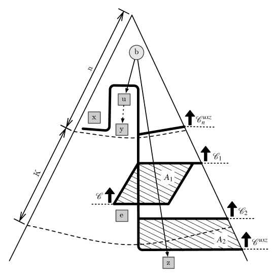
Figure 4: Rough sketch of the proof of Theorem 2; there exists a condition $b$ in the preset of both $u$ and $z$; moreover, $u<y$ and $n=\max(0pt{x},0pt{y})$. From $\mathcal{C}^{uxz}$ we construct the smaller configuration $\mathcal{C}$.

We now state the main result of this section:

Theorem 2

Let $N$ be a safe Petri net, $U$ its unfolding, and let $K$ as defined in (2). For any two events $x,y$ such that $\neg(x\mathbin{\triangleright}y)$, there exists an event $z$ such that

1. $\mathbf{wit}(x,y,z)$ and

2. $0pt{z}\leq n+K$, where $n:=\max(0pt{x},0pt{y})$.

Proof: The idea of the proof is illustrated in Figure 4. Let $f$ be the mapping between $N$ and $U$. If $\neg(x\mathbin{\triangleright}y)$ then some event $z$ satisfying $\mathbf{wit}(x,y,z)$ exists; it remains to determine the maximal height of $z$. If $x\mathbin{\#}y$, we are done immediately, taking $z:=x$. Otherwise, $\mathcal{C}_{xy}:=\lceil{x}\rceil\cup\lceil{y}\rceil$ is a configuration. Choose $z\in E$ such that $\mathbf{wit}(x,y,z)$ holds, and such that $z^{\prime}<z$ implies $\neg\mathbf{wit}(x,y,z^{\prime})$. By assumption we have $\neg(x\mathbin{\#}z)$, thus $\mathcal{C}_{xz}:=\lceil{x}\rceil\cup\lceil{z}\rceil$ is also a configuration. Further, let $u$ be such that $u\mathbin{\#}z$ and $u\leq y$ and such that $u^{\prime}<u$ implies $\neg(u^{\prime}\mathbin{\#}z)$. We claim that

$$\mathcal{C}^{uxz} := \lfloor{u}\rfloor\cup\lceil{x}\rceil\cup\lfloor{z}\rfloor$$

is a configuration: if this were not the case, then there would be events $e,e^{\prime}\in\mathcal{C}^{uxz}$ such that $e\mathbin{\#}e^{\prime}$. Since $\mathcal{C}_{xy}$ and $\mathcal{C}_{xz}$ are configurations, it would follow w.l.o.g. that $e\in\lfloor{u}\rfloor$ and $e^{\prime}\in\lfloor{z}\rfloor$, so $e<u$ and $e^{\prime}<z$. But then $e\mathbin{\#}z$ and $e^{\prime}\mathbin{\#}y$, both of which contradicts the minimality assumptions on $u$ and $z$. We thus have

$$\mathcal{C}^{uxz}\stackrel{{\scriptstyle z}}{{\leadsto}} \mathcal{C}^{uxz}\stackrel{{\scriptstyle u}}{{\leadsto}}\ .$$ and (3)

For $n=\max\{0pt{x},0pt{y}\}$, let $\mathcal{C}^{uxz}_{n}:=\{\,e\in\mathcal{C}^{uxz}\mid 0pt{\mathit{e}}\leq n\,\}$. Then $x\in\mathcal{C}^{uxz}_{n}$, and $\mathcal{C}^{uxz}_{n}\stackrel{{\scriptstyle u}}{{\leadsto}}$. Suppose that $z$ satisfies $0pt{z}>n+K$. Then the choice of $K$ implies the existence of two distinct configurations $\mathcal{C}_{1},\mathcal{C}_{2}$ of $U$ such that

1. $\mathcal{C}^{uxz}_{n}\sqsubseteq\mathcal{C}_{1}\sqsubseteq\mathcal{C}_{2}\sqsubseteq\mathcal{C}^{uxz}$,

2. $0pt{\mathcal{C}_{1}}<0pt{\mathcal{C}_{2}}$, and

3. $\mathit{Mark}(\mathcal{C}_{1})=\mathit{Mark}(\mathcal{C}_{2})$.

In fact, $\mathit{Mark}(\mathcal{C}_{1})=\mathit{Mark}(\mathcal{C}_{2})$ implies that $U/_{\mathcal{C}_{1}}$ and $U/_{\mathcal{C}_{2}}$ are isomorphic, and there exist sets $A_{1}$, $A_{2}$ with $f(A_{1})=f(A_{2})$ such that $\mathcal{C}_{2}\stackrel{{\scriptstyle A_{2}}}{{\leadsto}}\mathcal{C}^{uxz}$ and $\mathcal{C}_{1}\stackrel{{\scriptstyle A_{1}}}{{\leadsto}}\mathcal{C}$ for some $\mathcal{C}$. Now, $\mathit{Mark}(\mathcal{C})=\mathit{Mark}(\mathcal{C}^{uxz})$, so there exists an event $e$ such that $f(e)=f(z)$, $0pt{e}<0pt{z}$, and $\mathcal{C}\stackrel{{\scriptstyle e}}{{\leadsto}}$. Thus, $\mathcal{C}\cup\{e\}$ is a configuration containing both $x$ and $e$, so $\neg(x\mathbin{\#}e)$.

From $u\mathbin{\#}z$ and (3) it follows that $u$ and $z$ compete directly for a token, i.e. there exists a condition $b\in{{}^{\bullet}{u}}\cap{{}^{\bullet}{z}}$. Since $f(e)=f(z)$, there must be $b^{\prime}\in{{}^{\bullet}{e}}$ with $f(b^{\prime})=f(b)$. Now, $b\mathbin{\mathbf{co}}b^{\prime}$ cannot hold because $N$ is safe. Suppose $b\mathbin{\#}b^{\prime}$. But then there must exist two events $u^{\prime}\neq e^{\prime}$ such that $u^{\prime}<b$ and $e^{\prime}<b^{\prime}$ and ${{}^{\bullet}{u^{\prime}}}\cap{{}^{\bullet}{e^{\prime}}}\neq\emptyset$. By definition, $\mathcal{C}$ contains $\lfloor{u}\rfloor$ and enables $e$, so $b$ and $b^{\prime}$ must both be contained in the prefix $U[\mathcal{C}]$, so $u^{\prime},e^{\prime}\in\mathcal{C}$, but, being a configuration, $\mathcal{C}$ cannot contain two conflicting events. The only possibilities left are $b=b^{\prime}$, $b<b^{\prime}$, or $b^{\prime}<b$, and in all cases we obtain $e\mathbin{\#}u$ and therefore $e\mathbin{\#}y$.

We thus obtain $\mathbf{wit}(x,y,e)$, and the height of $e$ is strictly less than that of $z$. Either $0pt{e}\leq n+K$, and we are done; or we replace $z$ by $e$ and repeat the surgery above, obtain another witness with strictly lesser height etc, until we end up with a witness that has the desired height.           $\Box$

Theorem 2 in connection with Lemma 2 implies that for any pair $x,y$ of concurrent events, it suffices to inspect $U_{2}^{M_{xy}}$ to determine whether $x\mathbin{\triangleright}y$, where $M_{xy}:=M(\lceil{x}\rceil\cup\lceil{y}\rceil)$. Notice that this bound is much lower than the one given by Theorem 1; in fact, contrary to the previous bound it provides hope to actually compute the relation.

The reader will observe that in the proof of Theorem 2 we exploit the fact that a suffix of $\mathcal{C}_{n}^{uxz}$ with height $K$ contains two marking-equivalent causally related events. To find two such events, it actually suffices to search an isomorphic copy of the level-1 prefix starting at the marking associated with $\mathcal{C}_{n}^{uxz}$. It is thus tempting to think that Lemma 2 unfolds “one level too much”. However, for a given candidate $z$ as witness for $x$ and $y$, there may be many possible events $u$ for which one would have to search the suffix of $\mathcal{C}_{n}^{uxz}$, therefore limiting the candidates in this manner would not at all be straightforward. The value of Lemma 2 is in bounding the set of candidates for $z$ in a simple, effective manner.

4 Algorithms for computing the reveals relation

In this section, we exploit the results of Sections 2 and 3 to exhibit two concrete algorithms for determining the reveals relation. The main contribution is in Section 4.1, where we show how to compute the relation between all events in a given prefix. In Section 4.2 we discuss the question how to decide $x\mathbin{\triangleright}y$ for a single pair $x,y$.

4.1 Computing reveals on a given prefix

For the rest of this section, let us fix a finite occurrence net $O$, which should be a finite prefix of some safe Petri net, where $E$ is the set of events. We are going to compute the relation $\mathbin{\triangleright}$ between all pairs in $E$.

An algorithm for this purpose can be useful if either the underlying net is free of loops (and hence the unfolding is finite), or if one wants to compute the relation for all events of height up to $n$ (in which case the prefix should contain the events of height $n+K$).

Our algorithm consists of three passes over the occurrence net that compute, in turn, the causality relation $<$, the conflict relation $\mathbin{\#}$, and finally the reveals relation $\mathbin{\triangleright}$. We assume that events in $E$ are available in topologically sorted order, i.e. an order $\prec$ where $e<e^{\prime}$ implies $e\prec e^{\prime}$. Such an order can be easily established while scanning $O$: e.g., one first identifies the minimal conditions (those having no incoming arcs) and then traverses the unfolding with a standard worklist algorithm.

For the three passes that compute $<$, $\mathbin{\#}$, and $\mathbin{\triangleright}$, we exploit certain causal inheritance properties. It turns out that most operations can be implemented with simple bitset operations.

1. In the first pass, we compute for each event $e$ a set of events $\mathit{post}(e):=\{\,e^{\prime}\mid e\leq e^{\prime}\,\}$ containing its successors (and $e$ itself). Initially, that set is empty for all $e$; we then traverse $E$ in inverse topological order, exploiting the fact that the causal relationship is obviously transitive: $e\leq e^{\prime}$ iff $e=e^{\prime}$ or there exists $e^{\prime\prime}$ such that $e^{\prime\prime}\in{({e}^{\bullet})}^{\bullet}$ and $e^{\prime\prime}\leq e^{\prime}$.

2. In the second pass, we compute for each event $e$ the set $\mathit{conf}(e):=\{\,e^{\prime}\mid e\mathbin{\#}e^{\prime}\,\}$, i.e., the set of events with which $e$ is in conflict. Here, we exploit that the conflict relation is inherited by causal successors: $e\mathbin{\#}e^{\prime}$ iff ${{}^{\bullet}{e}}\cap{{}^{\bullet}{e^{\prime}}}\neq\emptyset$ or there exists $f$,$f^{\prime}$ such that $f\leq e$, $f^{\prime}\leq e^{\prime}$, and ${{}^{\bullet}{f}}\cap{{}^{\bullet}{f^{\prime}}}\neq\emptyset$. We traverse $E$ in topological order; each event $e$ inherits the conflicts of its (direct) causal predecessors and obtains new conflicts with the set $\mathit{post}(e^{\prime})$ for all events $e^{\prime}$ with which it directly competes for some condition.

3. In the third pass, we finally compute a set $\mathit{rev}(e)$ for each event $e$ such that $\mathit{rev}(e):=\{\,e^{\prime}\mid e\mathbin{\triangleright}e^{\prime}\,\}$. Here, we mainly exploit two facts: $e$ cannot reveal any events with which it is in conflict, and it reveals all events revealed by its causal predecessors: if $e^{\prime\prime}\mathbin{\triangleright}e^{\prime}$ and $e^{\prime\prime}<e$, then $e\mathbin{\triangleright}e^{\prime}$. We thus traverse $E$ in topological order; at each event, all known conflicts are discarded, and events from direct causal predecessors inherited. This leaves some events $e^{\prime}$ for which the status is unknown (concurrent events and causal successors), and for these we check directly whether $\mathit{conf}(e)\supseteq\mathit{conf}(e^{\prime})$ (compare Lemma 1).

Algorithm 1 Computing the reveals relation

  $\mathit{post}(e):=\{e\}$;  $\mathit{conf}(e):=\emptyset$;  $\mathit{rev}(e):=\{e\}$ for all $e\in E$

  for all $e\in E$ in inverse $\prec$-order do

     for all $e^{\prime}\in{{e}^{\bullet}}^{\bullet}$ do

        $\mathit{post}(e):=\mathit{post}(e)\cup\mathit{post}(e^{\prime})$

     end for

  end for

  for all $e\in E$ in $\prec$-order do

     for all $e^{\prime}\in{{}^{\bullet}{{{}^{\bullet}{e}}}}$ do

        $\mathit{conf}(e):=\mathit{conf}(e)\cup\mathit{conf}(e^{\prime})$

     end for

     for all $e^{\prime}$ s.t. ${{}^{\bullet}{e}}\cap{{}^{\bullet}{e^{\prime}}}\neq\emptyset$ do

        $\mathit{conf}(e):=\mathit{conf}(e)\cup\mathit{post}(e^{\prime})$

     end for

  end for

  for all $e\in E$ in $\prec$-order do

     for all $e^{\prime}\in{{}^{\bullet}{{{}^{\bullet}{e}}}}$ do

        $\mathit{rev}(e):=\mathit{rev}(e)\cup\mathit{rev}(e^{\prime})$

     end for

     $E^{\prime}:=E\setminus(\mathit{rev}(e)\cup\mathit{conf}(e))$;

     for all $e^{\prime}\in E^{\prime}$ do

        if $\mathit{rev}(e)\supseteq\mathit{rev}(e^{\prime})$ then

           $\mathit{rev}(e):=\mathit{rev}(e)\cup\{e^{\prime}\}$

        end if

     end for

  end for

Figure 1 shows a version of the algorithm in pseudo-code. Notice that if $\mathit{post}(\cdot)$, $\mathit{conf}(\cdot)$, and $\mathit{rev}(\cdot)$ are stored as bitsets (containing one bit for every event in $E$), then almost all operations can be implemented using basic logical operations on bitsets. In the first two passes, the number of such operations is bounded by the number of arcs in $U$. In the third pass, the number of operations is bounded by the pairs $(e,e^{\prime})$ such that $e^{\prime}\notin(\mathit{rev}(e)\cup\mathit{conf}(e))$, that is by $|E|^{2}$ in the worst case. However, it turns out that in most cases the number of such checks is comparatively small.

4.2 Computing reveals for a single pair

We briefly discuss the question of how to decide $x\mathbin{\triangleright}y$ for a single pair of events $x,y$. If one is interested in individual pairs, such a procedure may well be more efficient than the one from Section 4.1 because it allows to limit the events one has to consider.

Assume that $x,y$ are events of some unfolding $U$, of which at least the prefix $\lceil{x}\rceil\cup\lceil{y}\rceil$ is known. (We assume that neither $x\#y$ nor $x>y$ hold, otherwise the solution is trivial.) Denote by $\#_{\mu}[y]:=\{\,z\mid z\in\#[y]\land\forall z^{\prime}:(z^{\prime}<z\to z^{\prime}\notin\#[y]\,\}$ the set of $<$-minimal conflicts of $y$, its so-called root conflicts. Due to results from [12] we know that $x\mathbin{\triangleright}y$ iff $\#[x]\supseteq\#_{\mu}[y]$. To find a witness, it suffices therefore to find an event $z$ that is not in conflict with $x$, but a root conflict of $y$; the latter implies that ${{}^{\bullet}{z}}\cap\lfloor{y}\rfloor\neq\emptyset$.

We propose the following: First, mark the conditions in $\lfloor{y}\rfloor$ as ‘goals’. Secondly, mark all conditions and places in conflict with $x$ as ‘useless’ (they cannot produce a witness), as well as all elements of $\lfloor{x}\rfloor$ (which can equally not produce a witness by assumption). One then regards the remaining non-‘useless’ events up to the height given by Lemma 2, either by unfolding them on-the-fly or by following them on a pre-computed prefix. A witness is found if one such ‘non-useless’ events consumes a ‘goal’ condition.

5 Experiments

We implemented the theoretical and algorithmical results of the preceding sections and evaluated them experimentally. The problems we wanted to address were the following:

• What is the value of $K$ (as given by Lemma 2) for medium-sized nets?

• Provided a prefix is available, how efficiently can one determine $\mathbin{\triangleright}$, using Algorithm 1?

As inputs, we chose the safe Petri net examples supplied by the PEP tool [9]. Table 1 provides some statistics on the nets we used, such as the number of places and transitions, as well as the bound $K$ according to Lemma 2 for each particular net. We obtained $K$ by modifying the Mole unfolding tool [18]. Normally, Mole is used to compute finite complete prefixes; for our experiments, we modified its cutoff criterion so that it would compute the unfolding prefix $U_{2}$. We also give the time, in seconds, to compute the said prefix in the rightmost column.

Table 1: Net statistics and computation of $K$

Petri net	$|P|$	$|T|$	$K$	Time/s
buf100	200	101	201	2.1
elevator	59	74	80	0.3
gas_station	30	18	18	0.1
mutual	62	67	–	t/o
parrow	77	54	91	1.6
peterson	27	31	34	0.1
reader_writer_2	53	60	29	2.3
sdl_arq_deadlock	202	183	37	0.1
sdl_arq	208	234	129	0.2
sdl_example	323	471	71	0.1
sem	26	25	35	0.1

To make the experiments more interesting, we excluded non-cyclic examples, where $K$ would be obvious. For the rest, the computation of $K$ succeeded except in one case (mutual, more than 10 minutes). To give some indications, the size of a complete prefix in these cases was between several dozen and a few thousand events, whereas the size of $U_{2}$ was between several hundred and several ten thousands of events. By contrast, the computation of $K$ failed for another set of larger benchmarks provided by Mole, whose complete prefixes already have a size of 10,000 and more events.

To answer the second question, we implemented Algorithm 1 in Java. Our program took a pre-computed prefix and computed the relation $\mathbin{\triangleright}$ on it, using the BitSet class for most operations. The results are summarized in Table 2. As one can see, the algorithm works well even for several tens of thousands of events, usually computing the relation in a matter of seconds.

We detail the time for the three passes of the algorithm (all times are in seconds); in almost each case, we have the same ordering of computation times. The computation of the causal relation ($\mathit{post}$) takes hardly significant time, the second pass for the computation of the conflict relation ($\mathit{conf}$) takes a little more time, and the third pass for the computation of the reveals relation ($\mathit{rev}$) slightly dominates the computation time.

Table 2: Running times of Algorithm 1

Petri net	Events	post	conf	rev
		(Time/s)	(Time/s)	(Time/s)
bds_1.sync	12900	0.13	0.19	0.30
buf100	17700	0.17	0.12	0.25
byzagr4_1b	14724	0.18	0.19	0.68
dpd_7.sync	10457	0.11	0.15	0.24
dph_7.dlmcs	37272	0.56	0.91	2.10
elevator75	234879	15.84	22.58	97.47
elevator	5586	0.05	0.05	0.13
elevator_4	16856	0.17	0.27	0.38
fifo20	100696	2.92	3.72	22.88
ftp_1.sync	83889	2.08	3.61	6.78
furnace_3	25394	0.29	0.47	0.95
gas_station	2861	0.01	0.01	0.01
key_4.fsa	67954	1.40	2.19	4.62
parrow	85869	2.47	4.17	9.51
peterson	72829	1.60	2.54	5.23
q_1.sync	10722	0.11	0.15	0.30
q_1	7469	0.08	0.09	0.17
reader_writer_2	20229	0.24	0.37	0.53
rw_12.sync	98361	2.36	5.14	6.36
rw_12	49179	0.68	1.25	1.70
rw_1w3r	15401	0.15	0.22	0.50
rw_2w1r	9241	0.10	0.11	0.25
sdl_arq	2691	0.03	0.03	0.09
sem	19689	0.20	0.23	0.61

6 Conclusion

We presented theoretical and algorithmic contributions towards the computation of the reveals relation. The analysis in [12] had only provided the proof that $a\mathbin{\triangleright}b$ could be decided on some bounded prefix of the unfolding; but the bound (see Theorem 1) was prohibitively large, and an efficient procedure for computing $\mathbin{\triangleright}$ was lacking. The present paper closes this theoretical and practical gap. Our results show that with a suitable cutoff-criterion, the complete finite prefix $U_{2}$ is sufficient to obtain the $\mathbin{\triangleright}$-relation on $U_{1}$. Moreover, an efficient algorithm for computing $\mathbin{\triangleright}$ on finite occurrence nets has been proposed and tested; the experimental results clearly show that $\mathbin{\triangleright}$ can be obtained and used in practice.

The theory of reveals can be further developed in the lines of [2], where a dedicated logic (called ERL) is introduced for expressing generalized reveals relation of the form ”if all events from set A occur, then at least one event from set B must eventually occur”, and the problem of synthesizing occurrence nets from ERL formulas is solved. The study of further variants of logics for concurrency in the light of the recent results has only just begun.

In addition, we intend to extend reveals-based analysis to other Petri net classes such as Time nets and contextual nets, and to exploit it in applications that include diagnosis and testing.

References

- [1]
- [2] Sandie Balaguer, Thomas Chatain & Stefan Haar (2011): Building Tight Occurrence Nets from Reveals Relations. In: Proc. ACSD.
- [3] Albert Benveniste, Eric Fabre, Stefan Haar & Claude Jard (2003): Diagnosis of asynchronous discrete-event systems: a net unfolding approach. IEEE Transactions on Automatic Control 48(5), pp. 714–727, 10.1109/TAC.2003.811249.
- [4] Joost Engelfriet (1991): Branching Processes of Petri Nets. Acta Informatica 28(6), pp. 575–591, 10.1007/BF01463946.
- [5] Javier Esparza, Stefan Römer & Walter Vogler (2002): An Improvement of McMillan’s Unfolding Algorithm. Formal Methods in System Design 20(3), pp. 285–310.
- [6] Eric Fabre & Albert Benveniste (2007): Partial Order Techniques for Distributed Discrete Event Systems: Why You Cannot Avoid Using Them. Discrete Event Dynamic Systems 17(3), pp. 355–403, 10.1007/s10626-007-0016-1.
- [7] Eric Fabre, Albert Benveniste, Stefan Haar & Claude Jard (2005): Distributed Monitoring of Concurrent and Asynchronous Systems. Discrete Event Dynamic Systems 15(1), pp. 33–84, 10.1007/s10626-005-5238-5.
- [8] Ursula Goltz (1987): Synchronic distance. In: Advances in Petri nets 1986, part I on Petri nets: central models and their properties, Springer-Verlag, London, UK, pp. 338–358, 10.1007/BFb0046844. Available at http://portal.acm.org/citation.cfm?id=28641.28652.
- [9] Bernd Grahlmann (1997): The PEP tool. In: Computer Aided Verification, LNCS 1254, pp. 440–443, 10.1007/3-540-63166-6_43.
- [10] Stefan Haar (2007): Unfold and cover: Qualitative Diagnosability for Petri Nets. In: Proc. CDC, IEEE, pp. 1886–1891, 10.1109/CDC.2007.4434691.
- [11] Stefan Haar (2009): Qualitative Diagnosability of labeled Petri nets revisited. In: Proc. CDC, IEEE, pp. 1248–1253, 10.1109/CDC.2009.5400917.
- [12] Stefan Haar (2010): Types of Asynchronous Diagnosability and the Reveals-Relation in Occurrence Nets. IEEE Transactions on Automatic Control 55(10), pp. 2310–2320, 10.1109/TAC.2010.2063490.
- [13] Victor Khomenko, Maciej Koutny & Walter Vogler (2003): Canonical Prefixes of Petri Net Unfoldings. Acta Informatica 40(2), pp. 95–118, 10.1007/s00236-003-0122-y.
- [14] Kenneth L. McMillan (1992): Using Unfoldings to Avoid the State Explosion Problem in the Verification of Asynchronous Circuits. In: Proc. CAV, LNCS 663, Springer, pp. 164–177, 10.1007/3-540-56496-9_14.
- [15] Tadao Murata (1989): Petri nets: Properties, analysis and applications. Proc. IEEE 77(4), pp. 541–580, 10.1109/5.24143.
- [16] James L. Peterson (1981): Petri Net Theory and the Modeling of Systems. Prentice-Hall.
- [17] Wolfgang Reisig (1985): Petri Nets: An Introduction. Monographs in Theoretical Computer Science. An EATCS Series 4, Springer.
- [18] Stefan Schwoon: The Mole tool. http://www.lsv.ens-cachan.fr/~schwoon/tools/mole/.
- [19] Wen Zhao, Yu Huang & Chong-Yi Yuan (2008): Synchronic Distance Based Workflow Logic Specification. In: Proc. HPCC, pp. 819–824, 10.1109/HPCC.2008.48.