Anomalous scaling and generic structure function in turbulence

Abstract

We discuss on an example a general mechanism of apparition of anomalous scaling in scale invariant systems via zero modes of a scale invariant operator. We discuss the relevance of such mechanism in turbulence, and point out a peculiarity of turbulent flows, due to the existence of both forcing and dissipation. Following these considerations, we show that if this mechanism of anomalous scaling is operating in turbulence, the structure functions can be constructed by simple symmetry considerations. We find that the generical scale behavior of structure functions in the inertial range is not self-similar $S_{n}(\ell)\propto\ell^{\zeta_{n}}$ but includes an ”exponential self-similar” behavior $S_{n}(\ell)\propto\exp[\zeta_{n}\alpha^{-1}\ell^{\alpha}]$ where $\alpha$ is a parameter proportional to the inverse of the logarithm of the Reynolds number. The solution also follows exact General Scaling and approximate Extended Self-Similarity.

Résumé

A partir d’un exemple, nous discutons un mécanisme général de production de lois d’échelle anormales, dans un système invariant d’échelle. Ce mécanisme repose sur l’existence de valeurs propres nulles pour un opérateur invariant d’échelle. Nous discutons ensuite la pertinence de ce mécanisme en turbulence, en soulignant une particularité des écoulements turbulents, liée à la coexistence d’un forçage et de la dissipation. En utilisant ces considérations, nous montrons que si ce mécanisme s’applique à la turbulence, alors on peut construire les fonctions de structure par de simples arguments de symétrie. On trouve que le comportement générique des fonctions de structure n’est pas auto-similaire $S_{n}(\ell)\propto\ell^{\zeta_{n}}$ mais inclut un terme ”exponentiel auto-similaire” du type $S_{n}(\ell)\propto\exp[\zeta_{n}\alpha^{-1}\ell^{\alpha}]$, où $\alpha$ est un paramètre inversement proportionnel au logarithme du nombre de Reynolds. La solution satisfait également rigoureusement la propriété de Similarité Générale et approximativement la propriété d’Autosimilarité Etendue.

I Introduction

Anomalous scaling usually refers to situations where the observed scaling exponents deviate from their natural dimensional scaling. As a consequence, it is often associated with non-simple scaling behavior of the correlation functions: the scaling exponent of the 2n^th order correlation function is not $n$ times the scaling exponent of the 2^nd order correlation function. A good example of this situation is the scaling of the so-called velocity structure functions in 3D homogeneous isotropic turbulence. Dimensional considerations based on energy conservation K41 predict that the scaling exponent of the $n^{th}$ structure function should be $\zeta_{n}=n/3$. Observed scaling exponents substantially deviate from this prediction (see e.g. arneodo for a review of recent experimental results). Several general mechanisms of apparition of anomalous scaling have been identified. Among them, two mechanisms deserve special interest: existence of additional essential parameters which cannot be eliminated from the problem (this is the phenomenon of incomplete self-similarity, reviewed by barenblatt ) and existence of non-trivial zero modes of the closed equations satisfied by the correlation functions zeromodes .

Our aim is to study some consequences of these two form of anomalous scaling in situations where the system is scale invariant. Specifically, we show on a simple example how zero-modes give rise to a self-similar behavior of second kind. We then come back to the case of turbulence to show how this feature can be used to determine general properties of the scaling exponents and the scale behavior of the structure functions. The main conclusion of the present study is that the generic scale behavior of structure functions in the inertial range is not self-similar $S_{n}(\ell)\propto\ell^{\zeta_{n}}$ but ”exponential self-similar” $S_{n}(\ell)\propto\exp[\zeta_{n}\alpha^{-1}\ell^{\alpha}]$ where $\alpha$ is a parameter proportional to the inverse of the logarithm of the Reynolds number. The self-similar shape is recovered only in the limit of infinite size inertial range (infinite Reynolds number).

II Anomalous scaling in scale invariant systems

The goal of the present Section is not to prove rigorous results, but to illustrate a possible mechanism of generation of anomalous scaling in turbulence, and explore its consequences. In particular, the discussion about application to turbulence should be taken as rather speculative, since we do not derive any exact equations. The main goal of the present Section is to give justifications for the symmetry approach presented in the next Section, which will provide some new and quantitative results on structure functions in turbulence.

II.1 An example

Consider the differential equation:

$$\partial_{t}\phi+\partial_{\ell}\phi-\frac{\zeta}{\ell}\phi=F(\ell),$$ (1)

where $t$ is the time, $\ell$ is the scale, $\phi$ is a scale-dependent physical quantity (e.g. a structure function, or a correlation function), $F$ an external forcing and $\zeta$ a constant. We further assume that the scale range is bounded by some larger scale $L$, at which $\phi$ obeys the boundary condition $\phi(\ell=L)=0$, and that, for scales much smaller than the larger scale, $F$ follows a power-law $F(\ell)\propto\ell^{h_{0}}$. This property can be obtained for example if $F$ is a Gaussian random function with a power-law spectrum.

II.1.1 Scale invariance

We note that, in absence of forcing, ($F=0$), the equation (1) is invariant under the family of transformations ${\cal S}_{h}(\lambda)$:

$${\cal S}_{h}(\lambda):\;\ell\to\lambda\ell,\quad\phi\to\lambda^{h}\phi,\quad t\to\lambda t,$$ (2)

for arbitrary $\lambda$ and $h$. The physical system described by eq. (1) without forcing is then said to be scale invariant. Several important properties of scale invariant systems are listed in Section 3.1.

II.1.2 Zero-mode

In absence of forcing, stationary solutions of eq. (1) satisfy the homogeneous equation:

$$\partial_{\ell}\phi-\frac{\zeta}{\ell}\phi=0.$$ (3)

The solution is $\phi=A\ell^{\zeta}$, where $A$ is to be chosen according to the boundary condition, namely: $\phi(L)=AL^{\zeta}=0$, i.e. $A=0$. In absence of forcing, there are therefore no non trivial stationary solutions of eq. (1). The situation is modified when the forcing is taken into account.

II.1.3 Dimensional analysis

Before solving the forced equation, let us perform a simple dimensional analysis of eq. (1). We note that for scale smaller than $L$, stationary solutions can be found by using the scaling properties of $F$ (Section 2.1) and balancing the l.h.s. and the r.h.s. of (1):

$$\frac{\phi}{\ell}\sim F\sim\ell^{h_{0}},\;\ell\ll L,$$ (4)

which predicts another power-law solution $\phi\propto\ell^{1+h_{0}}$, for $\ell\ll L$.

II.1.4 Incomplete similarity

The previous dimensional analysis ignores the influence of the largest scale $L$. In fact, the solution must be influenced by the scale $L$, would it be only to satisfy the boundary condition $\phi(L)=0$ (which is not satisfied if the solution is only a power law!). A correct dimensional analysis thus imposes:

$$\phi(\ell)=\ell F(\ell)G(\ell/L),$$ (5)

where $G$ is a function which cannot be determined by dimensional arguments. A modification of the dimensional power law solution $\phi\propto\ell^{1+h_{0}}$ can then be observed if the variable $L$ is essential and if $G$ obeys incomplete similarity in $L$, i.e.:

$$G(\ell/L)\sim(\ell/L)^{-\Delta},\;L\gg 1,\;\Delta>0.$$ (6)

Since $\Delta$ is positive, the function $G$ tends to infinity when $L$ tends to infinity. In other words, the size of the system is always relevant and cannot be eliminated from the problem. In such a case, $\phi$ follows an anomalous scaling: $\phi\propto L^{\Delta}\ell^{1+h_{0}-\Delta}$. The value of $\Delta$ can be found by solving exactly the equation (1).

II.1.5 Exact solution of the complete problem

The stationary solution of eq. (1) is:

$$\phi=A\ell^{\zeta}+\ell^{\zeta}\int_{0}^{\ell}\rho^{-\zeta}F(\rho)d\rho.$$ (7)

The constant $A$ is found by imposing the boundary condition at $\ell=L$:

$$A=-\int_{0}^{L}\rho^{-\zeta}F(\rho)d\rho\sim L^{1+h_{0}-\zeta}.$$ (8)

The leading contribution to $\phi$ for $\ell/L\ll 1$ then depends on the sign of $\Delta=1+h_{0}-\zeta$. When it is negative, $\phi$ just obeys the dimensional scaling, and the contribution due to $L$ tends to zero as $L\to\infty$. This is the case of complete similarity, with no anomalous scaling. When $\Delta$ is positive, the dominant contribution is $L^{\Delta}\ell^{\zeta}$, which tends to infinity with $L$. This is the case of incomplete similarity described previously.

II.1.6 Summary

This simple example illustrates the general mechanism of anomalous scaling discussed in zeromodes in the case of a finite size, scale-invariant system: a zero mode, with a generic non-dimensional similarity exponent, and which does not satisfy the boundary condition, becomes relevant in the presence of an external forcing, which also imposes a dimensional, normal scaling exponent. The dominant contribution to the solution then depends on the relative value of the two scaling exponents, and in particular, on the behavior of the limit $L\to\infty$.

II.1.7 Implications on scaling exponents

In the case discussed previously, non-anomalous exponents are given by the exponents of the zero mode of a scale invariant differential operator. It then makes a lot of sense to investigate the possible constraints on scaling exponents dictated by the scale symmetry. This fully justifies computation of scaling exponents based on multi-fractal theory mfr , conformal theory polyakov , or more recently on a principle of exponent relativity developed in DG1 ; pocheau2 . Such approaches restrict more or less severely the possible shape of non-anomalous scaling in scale invariant systems. Restrictions are very weak in the case of the multi-fractal or conformal theory, while they are rather strong in the exponent relativity approach: in that case, the possible generic exponents fall into three classes depending on the properties of the rarest events. Within each class, the shape of the scaling exponents as a function of the order of the correlation function is entirely determined by the scale symmetry, and only depends on three parameters.

Transition from anomalous to non-anomalous scaling can also be constrained within the present model. Obviously, the value of the scaling exponents cannot be affected by modifications of external parameters, such as the strength of the force. The transition to non-anomalous scaling can only be obtained by a modification of the shape of the differential operator, i.e. by variation of internal parameters such as dimensionality, or isotropy properties. In the case of the white advected passive scalar, for example, it has been proved zeromodesbis that the non-anomalous behavior disappears in the limit where the (topological) dimension of the system is infinite. This kind of asymptotic behavior could well be found in a large variety of systems, such as turbulence.

II.2 The case of turbulence

The Navier-Stokes equations are:

$$\partial_{t}{\vec{u}}+({\vec{u}}\cdot{\vec{\nabla}}){\vec{u}}+{\vec{\nabla}}P=\nu\nabla^{2}{\vec{u}}+{\vec{F}},\quad{\vec{\nabla}}\cdot{\vec{u}}=0,$$ (9)

where $t$ is the time, ${\vec{u}}$ the velocity field, $P$ the pressure, $\nu$ the viscosity and ${\vec{F}}$ the external force, acting at large scales. Turbulence is defined as a statistically stationary regime of the Navier-Stokes equations where an external forcing balances the viscous energy losses and induces a constant energy rate: $du^{2}/dt=cte$. This means that the product ${\vec{F}}\cdot{\vec{u}}$ is scale independent, so that the force scales like $1/u$. We note that eq. (9) exhibits common features with eq. (1). The l.h.s. of (9) is invariant under the family of scale dilations ${\cal S}_{h}({\lambda})$ with arbitrary similarity exponent $h$ and scale factor ${\lambda}$ frischbook :

$${\cal S}_{h}({\lambda}):\quad{\ell}\to{\lambda}{\ell},\quad u\to{\lambda}^{h}u,\quad t\to{\lambda}^{1-h}t,$$ (10)

where $\ell$ is the space scale. This scale symmetry property is broken by both the forcing and the dissipation, which considered separately impose a dimensional scaling exponent: for the forcing, it is obtained by balancing $F$ and $du/dt$, which given the transformation properties of $F$, yields $u^{3}\sim\ell$, i.e. $h_{F}=1/3$. For the dissipation, balancing of $du/dt$ with $\nu\nabla^{2}u$ gives $u\sim\ell^{-1}$, i.e. $h_{D}=-1$.

Experimentally, none of these dimensional scalings is observed. Let us define the longitudinal velocity increments at scale $\ell$ by $\delta u_{\ell}={\vec{\ell}}\cdot[{\vec{u}}({\vec{x}}+{\vec{\ell}})-{\vec{u}}({\vec{x}})]/\ell$ and the velocity structure function of order $n$, $S_{n}(\ell)=<(\delta u_{\ell})^{n}>$, where $<>$ is a statistical average. In a range of scales small compared with the forcing scale, and large compared with the scales at which dissipation becomes non-negligible (the so called inertial range), the structure functions are observed to follow approximate power law behavior: $S_{n}(\ell)\propto\ell^{\zeta_{n}}$. The dimensional value imposed by the forcing would be $\zeta_{n}=nh_{F}=n/3$ while the dimensional value imposed by dissipation would be $\zeta_{n}=nh_{D}=-n$. Experimentally, none of these dimensional scaling is observed. The origin of this anomalous scaling can be understood within the mechanism explored previously: following the Navier-Stokes equation, the structure functions obey an equation of the type:

$$I_{n}S_{n}=F_{n}+D_{n},$$ (11)

where $I_{n}$ is a scale invariant differential operator acting in the scale space, and $F_{n}$ and $D_{n}$ contributions due to forcing and dissipation, imposing dimensional exponents $n/3$ and $-n$. The scaling exponents in the inertial range then come from the scaling properties of the zero-mode of the operator $I_{n}$. Note that until now, the explicit shape of the operator $I_{n}$ has never been computed, even perturbatively. It is quite possible that it is a non-diagonal operator of the structure functions, like in the Burgers equation, in which case the explicit computation of the zero-modes would be very difficult. Note also that for the Burgers equation, the scaling comes from the balance of non-diagonal contributions with terms corresponding to $D_{n}$, which shows that the anomalous scaling described in the previous Section does not necessarily apply for any type of equation. In this respect, our model equation (1) is a little bit ambiguous, and its application to turbulence not so straightforward as it may seem. We however adopt it as a working hypothesis, to explore its consequences.

Because of the presence of two scale-breaking symmetry mechanisms, turbulence offers a new possibility absent in the model equation (1): transition to new anomalous exponents at small scales, obtained by balancing of $F$ and $D$. Because of constant energy transfers, $F$ scales like $1/u$, while $D$ scales like $u/\ell^{2}$, so $h_{T}=1$. Indeed, experimentally, one observes a transition towards $S_{n}\propto\ell^{n}$ at small scales, the so-called “regular behavior”. The existence of this transition imposes a scale dependence for the scaling exponents, and thus, non trivial scale dependence for the shape of the structure functions. Of course, this shape depends both on the shape of the operator $I_{n}$, and on $F_{n}$ and $D_{n}$. Given the symmetry properties of $I_{n}$, it is however interesting to investigate whether the scale symmetry does impose possible generic shape for the structure functions, even within the inertial range, in the same way as it does constrain the $n$ dependence of the scaling exponents. This is the purpose of the next Section.

III Scale covariant structure functions in turbulence

In the present Section, we assume that the velocity structure functions in turbulence obey a differential equation which can be put under the form (11), where $I_{n}$ is a scale invariant operator. Furthermore, we assume that the solution in the inertial range is given by the homogeneous part of the equation ($F_{n}=D_{n}=0$), and that there is a transition towards the ”regular” solution $S_{n}(\ell)=K_{n}\ell^{n}$ at a scale $\ell=\eta_{n}$, where both $K_{n}$ and $\eta_{n}$ are entirely determined by $F_{n}$ and $D_{n}$. Our inertial range solution therefore extends up to $\eta_{n}$. Our aim is to derive a generic shape for the structure functions, satisfying all these requirements. From now on, we focus on stationary situations, thereby neglecting any time dependence.

III.1 On scale symmetry

A scale invariant system is according to our definition, invariant by a transformation ${\cal S}_{h}(\lambda)$ given in (2). Note that in log-variables $A=\ln\phi$, $T=\ln\ell$, this transformation amounts to a translation invariance in $A$ and $T$. This symmetry is rather intuitive, and connected with the possibility to multiply any characteristic quantity by an arbitrary constant, i.e. to perform arbitrary changes of units in the system DG1 . This corresponds to a global scale invariance. In fact, as discussed by Pocheau pocheau , scale symmetry encompasses another notion, corresponding to symmetry with respect to local scale dilations. This symmetry is connected with the invariance of the system with respect to changes of resolution, or equivalently to the possibility of performing arbitrary changes of rationalized (power law) unit systems DG1 . To understand this local symmetry, it is convenient to consider a discrete slicing of the space scale $\ell\leq L$, under the form:

$$\ell_{i} = \Gamma^{i}\ell_{0},\quad\phi_{i}=\Lambda^{i}\phi_{0},$$

$$L = \Gamma^{N}\ell_{0}.$$ (12)

Here, $\Gamma$ (or equivalently $N$) and $\Lambda$ characterize the resolution of the observations. By local scale symmetry, we require that the system be invariant by changes of resolution, i.e. by changes of $N$. Changes in $N$ are achieved by dilations of $\Gamma$: $\Gamma\to\Gamma^{\alpha}$, which transform $i$ into $i\alpha$. It is also a transformation which transform $\ell_{i}/\ell_{j}$ into $(\ell_{i}/\ell_{j})^{\alpha}$, and $\phi_{i}/\phi_{j}$ into $(\phi_{i}/\phi_{j})^{\alpha}$. A local scale dilation can therefore be seen as a transformation:

$$\ell/\ell_{0}\to(\ell/\ell_{0})^{\alpha},\quad\phi/\phi_{0}\to(\phi/\phi_{0})^{\alpha},$$ (13)

for arbitrary $\alpha$, $\ell_{0}$ and $\phi_{0}$. It can be seen as a change of rationalized unit system because it amounts to change $\ell_{0}$ and $\phi_{0}$ by $\ell_{0}(\ell/\ell_{0})^{1-\alpha}$ and $\phi_{0}(\phi/\phi_{0})^{1-\alpha}$.

Summarizing, we say that a system is scale invariant, if it is invariant under both (2) and (13), i.e. if the equations governing its evolution are covariant (keep the same shape) under these two transformations.

III.2 Generic equation for structure function

Assuming that a turbulent flow is scale invariant, we must then write the equations followed by a structure function $S_{n}(\ell)$ in a covariant way. For convenience, we introduce the log variables $X_{n}=\ln S_{n}$ and $T=\ln\ell$ remark0 . The shape of the structure function is determined by the function $X_{n}(T)$, given some boundary (initial) conditions. We must write the differential equation followed by $X_{n}$. Because of the global symmetry (2), which amounts to a translation invariance in $X_{n}$ and $T$, this differential equation can only include derivatives of $X_{n}$ with respect to $T$. In the spirit of the amplitude equation theory, we write the generic equation as an expansion in power of the amplitude:

$$\chi_{n} = a_{n}\frac{dX_{n}}{dT}+b_{n}\frac{d^{2}X_{n}}{dT^{2}}+c_{n}\frac{d^{3}X_{n}}{dT^{3}}+O(\frac{d^{4}X_{n}}{dT^{4}})$$ (14)

$$+ g_{n}\biggl{(}\frac{dX_{n}}{dT}\biggr{)}^{2}+h_{n}\frac{dX_{n}}{dT}\frac{d^{2}X_{n}}{dT^{2}}+O((\frac{dX_{n}}{dT})^{3}),$$

where $\chi_{n}$,$a_{n}$, $b_{n}$, …$h_{n}$ are some $T$ independent constants characterizing the system and are to be chosen in order to respect the local scale symmetry. Applying the transformation (13) to (14), we see that this equation is covariant only if the constants satisfy the following transformation rule:

$$\chi_{n}\to\chi_{n};\;a_{n}\to a_{n};\;\;b_{n}\to\alpha b_{n};c_{n}\to\alpha^{2}c_{n};$$

$$g_{n}\to g_{n};\;h_{n}\to\alpha h_{n};...$$ (15)

This suggests to introduce two characteristic constant scales in the system, $\ell_{0}$ and $\ell_{1}$ and to write:

$$\chi_{n} = {\tilde{\chi}_{n}},$$

$$a_{n} = {\tilde{a}_{n}},$$

$$b_{n} = {\tilde{b}_{n}}\ln(\ell_{1}/\ell_{0}),$$

$$c_{n} = {\tilde{c}_{n}}(\ln(\ell_{1}/\ell_{0}))^{2},$$

$$g_{n} = {\tilde{g}_{n}},$$

$$h_{n} = {\tilde{h}_{n}}\ln(\ell_{1}/\ell_{0}),$$ (16)

where the constants ${\tilde{\chi}_{n}},...$ are invariant under the local scale transformation, and only depend on the structure function (i.e. on $n$) and on the choice of $\ell_{0}$ and $\ell_{1}$. From now on, we fix the scale origin at the integral scale $\ell=L$ (representing the largest correlated motions). With this choice, scale invariance symmetry holds for

$$-\ln(R_{*})\leq T\leq 0,$$ (17)

where $R_{*}=L/\eta$ is a dimensionless number apparented to a Reynolds number and $\eta$ is. the Kolmogorov scale (representing dissipative scales of turbulence).

III.3 The case of turbulence

Equation (14), with constants following (16) is a generic equation in a scale invariant system, satisfying both global and local symmetry. Its solution depends on the values of the constants, which must be computed following some systematic procedure. However, interesting features of the solution may already be found in the linear approximation, where all terms of degree $A^{2}$ or higher are neglected remark2 . This approximation may be justified by considering a range of scales where the amplitude $A$ is small enough. We study here only the simplest case relevant to turbulence.

III.3.1 The linear case

The highest relevant derivative is determined by the number of boundary conditions. The existence of a largest scale in the system (e.g. the injection scale) imposes already at least one boundary condition. Furthermore, the existence of the transition between the scale invariant solution and the regular solution at $\ell=\eta_{n}$ imposes at least a second boundary condition. Note that this is a peculiarity of turbulence. In many scale invariant systems, only one boundary condition is needed, corresponding to an infrared or ultraviolet cut-off in the scale space.

We adopt $L$, the integral scale scale, and $\eta_{n}$ to normalize the constants, and introduce the pseudo-Reynolds number

$$\ln(R_{n})=\ln(L/\eta_{n}).$$

Dropping tildes for convenience, we therefore write the simplest differential equation relevant to structure functions in turbulence as:

$$\chi_{n}=a_{n}\frac{d\ln(S_{n})}{dT}+b_{n}\ln(R_{n})\frac{d^{2}\ln(S_{n})}{dT^{2}},$$ (18)

where $\chi_{n}$, $a_{n}$ and $b_{n}\neq 0$ are $T$ independent constant depending on the order of the structure function. Note that they also are independent on the Reynolds number, since solutions with different Reynolds number $R_{1}$ and $R_{2}$ can be related by a local scale transformation (13) with $\alpha=\ln(R_{1})/\ln(R_{2})$. The solution is:

$$\ln(S_{n}) = \frac{\chi_{n}}{2b_{n}\ln(R_{n})}T^{2}+\alpha_{n}T+\beta_{n},\quad a_{n}=0,$$

$$\ln(S_{n}) = \frac{\chi_{n}}{a_{n}}T+\alpha_{n}e^{-(a_{n}T)/(\ln(R_{n})b_{n})}+\beta_{n},\quad a_{n}\neq 0.$$ (19)

The constant $\alpha_{n}$ and $\beta_{n}$ are fixed by the boundary conditions. Without loss of generality, we can fix the scale origin at $\ell=L$, and choose the normalization for $S_{n}$ such that:

$$\ln(S_{n})(T=0) = 0,$$

$$\frac{d\ln(S_{n})}{dT}|_{T=-\ln(R_{n})} = n.$$ (20)

The second boundary condition guarantees the transition towards the regular solution. These boundary conditions fix the constants as:

$$\alpha_{n} = n+\frac{\chi_{n}}{b_{n}};\;\beta_{n}=0,\quad a_{n}=0,$$

$$\alpha_{n} = -\beta_{n}=\biggl{(}\frac{\chi_{n}}{a_{n}}-n\biggr{)}\frac{b_{n}\ln(R_{n})}{a_{n}}e^{-a_{n}/b_{n}},\quad a_{n}\neq 0.$$ (21)

The solutions (19) with constant given by (21) both follow the behavior schematized in Fig. 1: a power law behavior around $\ell=L$, followed by a transition regime towards $\ell=\eta_{n}$, where matching with the regular solution is obtained.

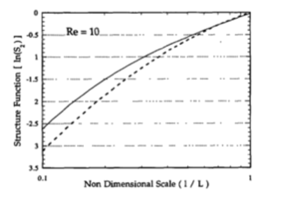
Figure 1: The behavior of a structure function versus the scale when $a_{n}=0$ (dotted line) and $a_{n}\neq 0$ (continuous line).

The second solution, with $a_{n}\neq 0$ (generic case) is the most interesting, because it exhibits a feature reminiscent of what is observed in turbulence. This is the subject of the remaining Sections.

III.3.2 Large Reynolds number limit

In the limit where the pseudo-Reynolds number is very large, $T/\ln(R_{n})\ll 1$ and the argument of the exponential can be expanded. The generic solution then approaches the self-similar behavior:

$$\ln(S_{n})=\biggl{(}\frac{\chi_{n}}{a_{n}}(1-e^{-a_{n}/b_{n}})+ne^{-a_{n}/b_{n}})\biggr{)}\ln(\ell/L).$$ (22)

This behavior is also valid in the neighborhood $\ell=L$. This kind of asymptotic behavior has been observed in a tunnel wind experiment by Castaing et al castaingetal : when the Reynolds number is increased, the shape of the structure function goes from exponential power law, like in the first part of our generic solution (19b), to self-similar power law behavior. Even in the moderate Reynolds number regime, Castaing and his collaborators observe that the exponential power law regime is superseeded at larger scales by a pure power law regime. Such kind of behavior is indeed obtained at $\ell>L$ in the generic solution, provided $a_{n}/b_{n}$ is negative. This exponential power law as well as the variation of the exponent with ($1/\ln R$) has also been predicted by Castaing castaing using a scale invariant Lagrangian formalism and requirement of finite dissipation. Within the present framework the result appears to stem both from scale invariance and finite size effects (see discussion).

III.3.3 Interpretation of the constants

Up to this stage, we have not tried to characterize the various constants $\chi_{n}$, $a_{n}$ and $b_{n}$ appearing in the solution. They should in principle be directly computed from the Navier-Stokes equations. Given the properties of the generic solution, we can however propose an interpretation of the constants which provides some constraints on their shape. Consider the asymptotic behavior of the solution (22). It defines some ”inertial range” scaling exponents:

$$\zeta_{n}=ne^{-a_{n}/b_{n}}+\frac{\chi_{n}}{a_{n}}(1-e^{-a_{n}/b_{n}}).$$ (23)

They are made from two contributions: one stemming from the solution of the equation $dA/dT=\chi_{n}/a_{n}$; another one coming from the exponential power term, present only when $b_{n}$ is different from zero, i.e. when the system is of second order. As discussed in Section 3, the presence of this term is directly linked with the existence of a small scale cut-off, where the solution must bifurcate towards the regular solution. It can therefore be interpreted as a finite-size effect. On the other hand, the contribution at $b_{n}=0$ characterizes a perfect scale invariant solution, extending from $0$ to infinity in the scale space. This separation is reminiscent of the model of Dubrulle and Graner DG1 , in which generic scaling exponents can be written:

$$\zeta_{n}=n\Delta_{\infty}+\delta\zeta_{n}.$$ (24)

Here, $\delta\zeta_{n}$ is a contribution stemming only from scale symmetry considerations. It is characterized by its large $n$ limit $C=\lim_{n\to\infty}\delta\zeta_{n}$ which can be interpreted as the codimension of the most intermittent structures. The term proportional to $\Delta_{\infty}$ is the contribution due to the scaling properties of the maximum value of $\ln(S_{n})$, which is defined only for finite-size systems. The factorization (24) with a linear dependence of the contribution due to finite-size effect can also be justified from dynamical considerations ugalde . This suggests to interpret the constants appearing in (23) as:

$$e^{-a_{n}/b_{n}} \equiv \Delta_{\infty},$$

$$\frac{\chi_{n}}{a_{n}} \equiv \frac{\delta\zeta_{n}}{1-\Delta_{\infty}}.$$ (25)

With this interpretation, finite size effects modifies the scale invariant solution in two ways: by the introduction of the linear term $n\Delta_{\infty}$ and by the modification of the codimension of the most intermittent structure:

$$C_{scale}=\frac{C_{finite}}{1-\Delta_{\infty}},$$ (26)

where $C_{scale}$ is the codimension in the scale invariant case, and $C_{finite}$ is the codimension in the finite size case. We stress that this finite size effect is Reynolds number independent (it only depends on the value of the constant $b_{n}$). It may however depend on other external parameter, such as the dimension (see discussion of Section 2.1).

Using eq. (21), interpretation (26) completely determines the ratio $\chi_{n}/a_{n}$ and $a_{n}/b_{n}$ as a function of $\Delta_{\infty}$ and the function $\delta\zeta_{n}$, which can be severly constrained using only scale symmetry requirements DG1 .

III.3.4 Example: log-Poisson case

As an example, let us considered the case where $\delta\zeta_{n}$ corresponds to a log-Poisson statistics SL ; dubrulle ; SW ; DG2 (one of the three possible cases derived in DG1 ):

$$\delta\zeta_{n}=C(1-\beta^{n}),$$ (27)

where $C$ and $\beta$ are two constants. If we adopt the values $C_{finite}=2$, $\beta^{3}=2/3$ and $\Delta_{\infty}=1/9$ as advocated by She and Leveque SL , for high Reynolds number turbulence, we can numerically determine the values of all parameters and thus, the scale dependence of the structure functions, providing the pseudo-Reynolds number $R_{n}$ are given. Table 1 summarizes the values obtained for $n=2$ to $6$. The corresponding structure functions, for $R_{n}=10$ are given in Fig. 2.

$n$	$\chi_{n}/a_{n}$	$a_{n}/b_{n}$
2	0.53	2.2
3	0.75	2.2
4	0.95	2.2
5	1.1	2.2
6	1.25	2.2

Table 1: Values of the parameters appearing in the structure functions for the log-Poisson model.

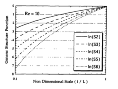
Figure 2: The generic structure functions $S_{2}$ to $S_{6}$ in the log-Poisson case.

III.3.5 Comparison with Batchelor’s parametrization

Using only symmetry arguments, we derived the shape of the structure functions in the linear approximation. This shape can be compared with the Batchelor’s parametrization, which can be derived from the Kolmogorov four-fifth law using matched asymptotics. This parametrization gives:

$$S_{2}(\ell)=\frac{A(\ell/\eta)^{2}}{\biggl{[}1+B(\ell/\eta)^{2}\biggr{]}^{(2-\zeta_{2})/2}},$$ (28)

where $A$ and $B$ are constants depending on the skewness of the velocity derivatives ($B\approx 7.2\times 10^{-3}$ stolo ). The best fit between Batchelor’s parametrization and the generic solution is obtained for $\eta_{2}=6.35\eta$ and is shown in Fig. 3.

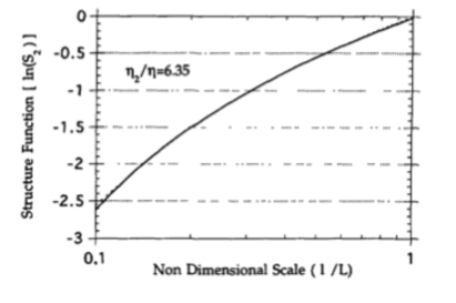
Figure 3: Comparison between the Batchelor parametrization (dotted line) and the generic structure function $\ln(S_{2})$ in the log-Poisson case (continuous line).

III.3.6 General scaling

The structure functions computed in the previous Section display an interesting property, referred to in turbulence as General Scaling (GS) GS . We introduce the maximal event function $S_{\infty}$ defined as:

$$S_{\infty}=\lim_{n\to\infty}\frac{S_{n+1}}{S_{n}}.$$ (29)

In a bounded system, this function is always defined and represents the event of maximal intensity. In turbulence, it represents the largest velocity differences. The reduced structure functions $S_{n}/S_{\infty}^{n}$ then obey a remarkable factorization property,

$$\ln\biggl{(}\frac{S_{n}}{S_{\infty}^{n}}\biggr{)}\propto\ln\biggl{(}\frac{S_{3}}{S_{\infty}^{3}}\biggr{)}.$$ (30)

This is shown in Fig. 4a. This factorization property, extending throughout the whole scale interval, can be seen as a generalization of the factorization occurring in the inertial range, where all structure functions are proportional to $T$.

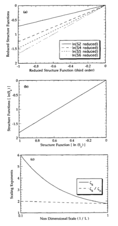
Figure 4: Top: (a) General Scaling: all the reduced structure functions are proportional to each other (here the third one). Middle: (b) Extended Self Similarity: when the $6^{th}$ order structure function is plotted against the $3^{rd}$ one, one observes a better defined scaling regime (compare with Fig. 2). Despite the visual impression, the Extended Self Similarity is only approximate (see Section 3). Bottom: (c) Local scaling exponent $\zeta_{6}$ and relative scaling exponent $\zeta_{6}/\zeta_{3}$ versus the scale. The local scaling exponent decreases constantly with the scale, proving the absence of exact self-similarity. By contrast, the relative scaling exponent varies much less, which enables a better determination of this exponent (ESS property).

This result can be explained by our choice of $n$ independent pseudo-Reynolds numbers $R_{n}\equiv R$. In such case, from (19) and (25), we obtain:

$$\ln(S_{\infty})=\Delta_{\infty}\frac{\ln(R)}{\ln(\Delta_{\infty})}\biggl{(}\Delta_{\infty}^{T/\ln(R)}-1\biggr{)}.$$ (31)

The reduced structure functions $S_{n}/S_{\infty}^{n}$ are then simply given by:

$$\ln\biggl{(}\frac{S_{n}}{S_{\infty}^{n}}\biggr{)}=\frac{\delta\zeta_{n}}{1-\Delta_{\infty}}\biggl{[}T-\Delta_{\infty}\frac{\ln(R)}{\ln(\Delta_{\infty})}\biggl{(}\Delta_{\infty}^{T/\ln(R)}-1)\biggr{]},$$ (32)

and are proportional to each other within the whole scale interval. It is not clear whether the present analysis provides an explanation to the GS observed in turbulence. It is not known in turbulence whether the pseudo-reynolds numbers $R_{n}$ are actually $n$ independent, i.e. if the transition from inertial range solution towards the regular solution occurs at the same scale $\eta_{n}=\eta$ (see GS for a discussion about $n$ dependent cut-offs). If the dependence of $\ln(R_{n})$ with $n$ is weak, as seems to be the case in turbulence, then the present analysis is still valid in turbulence and explains the phenomenon of GS within the context of scale symmetry.

III.3.7 Extended Self-Similarity

The factorization property (30) can be strengthened if, in addition, $\ln(S_{\infty})$ is also proportional to any $\ln(S_{n}/S_{\infty}^{n})$. In that case GS , the logarithms of any structure functions are proportional to each other. In other words, when one structure function is plotted against another one (e.g. the third one), one observes a well defined scaling regime, even in the range of scale where the function is not self-similar. This property was called Extended Self-Similarity ESS . The condition to observe this is $\Delta_{\infty}\to 0$. In practise, if this condition is satisfied approximately, one can expect to observe ESS in the system. In our case, $\Delta_{\infty}=1/9$ is small, so we should observe ESS. This is illustrated in Fig. 4b. Note that ESS property means that the relative exponent $\zeta_{n}^{\star}$ defined as

$$\zeta_{n}^{\star}=\frac{d\ln(S_{n})}{d\ln(S_{3})},$$ (33)

is much better defined than the true exponent:

$$\zeta_{n}=\frac{d\ln(S_{n})}{d\ln(\ell)}.$$ (34)

To illustrate this point, we have computed these scaling exponents for $n=6$ (Fig. 4c). It can be seen that $\zeta_{6}$ decreases steadily from $\zeta_{6}=6$ to $\zeta_{6}=1.78$, while $\zeta_{6}^{\ast}$ displays much weaker variations over the whole interval, from $\zeta_{6}^{\ast}=2$ to $\zeta_{6}^{\ast}\approx 1.8$ (the “intermittent value”).

III.3.8 Finite size effects vs asymptotic K41 solution?

In the previous Sections, we have used an interpretation of the constants to compute explicitly structure functions. This interpretation was dictated by our choice to introduce explicitly the dissipative range in the boundary condition (via the matching to the “regular solution”). In such interpretation, asymptotic (high Reynolds number) scaling exponents take the shape (23), with a linear part coming explicitly from finite size effects. In absence of finite size effects, they take the simple shape $\zeta_{n}=C_{scale}(1-\beta^{n})$ predicted by Dubrulle and Graner DG1 . The Kolmogorov solution $\zeta_{n}=n/3$ is never reached, unless the coefficient $\beta$ appearing in (19b) depends on other external parameters such as the dimension. The Kolmogorov solution could then appear as the infinite dimension limit (even in presence of finite size effects), and $\beta$ would be a parameter characterizing the dimension of the system.

Other interpretations are however possible, within the same symmetry arguments. For exemple, one could restrict the solutions to an “inertial range” of scale defined by imposing $\zeta_{3}=1$, i.e. $\alpha_{3}=0$ in (27). Asymptotic Kolmogorov solution could then be obtained with the following choice of constants (still compatible with the theory of Dubrulle-Graner):

$$\frac{\chi_{n}}{a_{n}} \equiv \frac{\delta\zeta_{n}}{\delta\zeta_{3}},$$

$$-\alpha_{n}\frac{a_{n}}{b_{n}\ln(R_{n})} \equiv \frac{n}{3}-\frac{\delta\zeta_{n}}{\delta\zeta_{3}},$$

$$e^{-a_{n}/b_{n}} = 3\Delta_{\infty}.$$ (35)

In such case, the derivative $d\ln(S_{n})/dT$ reaches the value (24) at $T=\ln(R_{n})$, which appears as another boundary condition. In absence of finite size effects, the scaling exponents are $\zeta_{n}=(1-\beta^{n})/(1-\beta^{3})$. The Kolmogorov solution $\zeta_{n}/3$ is obtained as the asymptotic solution (Reynolds tends to infinity) in presence of finite size effects.

We were not able to discriminate between these two types of interpretations. Obviously, one is rather valid in the vicinity of the dissipative range. It could then be seen as a refinement of the arguments by Frisch and Vergassola FV obtained within the multifractal model (see castaingetal for a discussion within the log-similarity hypothesis). The second is valid in the “inertial range”, defined using $\zeta_{3}=1$ (inertial range log-similarity hypothesis, see castaingetal ). They however lead to distinct prediction about the possibility to approach Kolmogorov solution. The most recent experimental results seem to indicate that the observed scaling exponents are almost independent of the Reynolds number arneodo . This would favor the first interpretation, and explain our choice in the present paper. Obviously, it would be interesting to consider further the variation of scaling exponents with the Reynolds number, and, possibly, to reconsider the second interpretation.

It should be stressed however that in any case, the “exponential power-law” appears as a prediction of symmetry arguments, independent of any boundary consideration, i.e. of these kind of interpretations.

IV Discussion

Using only symmetry considerations, we were able to build generic structure functions reproducing many features observed in actual structure functions in turbulence: transition from exponential power shape to a power shape with increasing Reynolds number, extended-self-similarity, regular matching with the regular solution at small scale. We do not claim that the generic structure functions considered in the present paper actually fit exactly the structure functions determined experimentally, because we intentionally considered only the simplest case relevant to turbulence, where the equation is linear. It is clear for example that the observed large scale saturation of the structure functions, which is absent in the linear model, could be obtained by taking into account non-linear terms in the differential equation, i.e. by a slightly more complicated model.

Our results illustrate the essential influence of scale symmetry on structure functions in turbulence, and provides further support to the scenario of ”scale invariant” anomalous scaling discussed in Section 2. We note that finite size effects (ultraviolet cut-off) generically lead to non-power law behavior of the structure function, but rather to exponential power-law behavior, $\exp(\ell^{\alpha})$, where $\alpha$ is real, proportional to the inverse Reynolds number. Such dependence, connected with the requirement of covariance by resolution, was also inferred by Barenblatt and Goldenfeld using the principle of ”Reynolds number covariance” barenblatt2 . We see here that such principle (left unjustified by Barenblatt and Goldenfeld) is directly connected with scale symmetry. Finally, we note that there is a possibility to get complex exponential power-law behaviors ($\alpha$ complex) if we allow a differential equation of higher order, or if we allow the presence of terms directly proportional to $A$ in (14). The first possibility could be justified if more than two boundary conditions are necessary to specify the solution. The second possibility still requires only two boundary conditions, but implies a breaking of global scale invariance. This requires the existence of a privileged scale into the system, and occurs for example in a system subject only to discrete scale invariance sornette . Complex exponents gives rise to log-periodic oscillations at large Reynolds number (when the solution goes from exponential power law to power law), which may have been detected in a variety of physical systems sornette ; TB . It would be interesting to see whether they can also arise in certain turbulent flows.

Acknowledgements

We thank F.M Bréon for assistance in the preparation of the manuscript and M. Vergassola and G. He for useful comments. This work was supported by a grant from the french Caisse d’Allocations Familiales.

References

- (1) Kolmogorov, A.N., 1941. C.R. Acad. Sci. URSS, 30, 301-305.
- (2) Arnéodo, A. et al. (1996) Europhys. Letter 34 6 411-416.
- (3) Barenblatt, G.I. Similarity, Self-Similarity and Intermediate Asymptotics, Plenum, New York, 1979.
- (4) Chertkov, M., Falkovich, G., Kokolov, I. and Lebedev, L. Phys. Rev. E, 52, 4924 (1995); Gawedzki, K. and Kupiainen, A., Phys. Rev. Letters, 75, 3834, (1995); Shraiman, B. and Siggia, E., C.R. Acad. Sci., 321, Série II, 279, (1995); Vergassola, M. Phys. Rev E, 53 R3021 (1996).
- (5) Parisi, G. and Frisch, U. in Turbulence and Predictability in Geophysical Fluid Dynamics, Varenna, Italy, 84, eds. M. Ghil, R. Benzi and G. Parisi, North-Holland, Amsterdam, 1985.
- (6) Polyakov, A.M. Nucl. Phys., B396, 367, (1993).
- (7) Dubrulle, B. and Graner, F. J. Physique II France 6 797 (1996).
- (8) Pocheau, A., Europhys. Letters, 35 183 (1996).
- (9) Bernard, D., Gawedzki, K. and Kupiainen, A. preprint IHES (1996).
- (10) Frisch U. Turbulence. Cambridge University Press, (1995).
- (11) Note that until now, the explicit shape of the operator has never been computed, even perturbatively.
- (12) Pocheau A. Phys. Rev. E, 49, (1994), 1109.
- (13) Because if the global scale invariance, it does not matter whether we work with or with , where is any characteristic scale.
- (14) Note that a linear equation in the variable is not necessarily linear in the variable .
- (15) Castaing, B., Gagne, Y. and Marchand, M. Physica D 68 387, (1993).
- (16) Chabaud, B., Naert, A., Peinke, J., Chilla, F., Castaing, B., and B. Hébral Phys. Rev. Lett. 73 3227, (1994).
- (17) Ugalde, E. and Lima, R. preprint CPT (1996).
- (18) She, Z-S., Leveque, E. 1994. Phys. Rev. Lett. 74, 262-265.
- (19) Dubrulle, B., 1994. Phys.Rev. Lett. 73, 7, 959-962.
- (20) She, Z-S., Waymire, E.C., (1995) Phys. Rev. Letters 75 274-279.
- (21) Dubrulle, B. and Graner, F. J. Physique II France 6 817 (1996).
- (22) Stolovitzky, G., Sreenivasan, K.R. and Juneja, A., (1993) Phys. Rev. E, 48, 5, R3217-R3220.
- (23) Benzi, R., Ciliberto, S., Tripiccione, R., Baudet, C., Massaioli, F., Succi,S., 1993. Physical Review E, 48, 1, R29-R32.
- (24) Benzi, R., Biferale, L., Ciliberto, S., Struglia, M. and Tripiccione, R. submitted to Physica D (1996).
- (25) Frisch, U. and Vergassola, M., (1991) Europhys. Letter 14, 439.
- (26) Barenblatt, G.I; and Goldenfeld, N., Phys. Fluids 7 3078, (1995).
- (27) Saleur, H., Sammis, C.G. and D. Sornette, J. Geophys. Research, 101 17661 (1996).
- (28) Graner, F. and Dubrulle, B. Astron. Astroph. 282 262 (1994).