TeV and Multi-wavelength Observations of Mrk 421 in 2006-2008

Abstract

We report on TeV $\gamma$-ray observations of the blazar Mrk 421 (redshift of $0.031$) with the VERITAS observatory and the Whipple $10\,\rm{m}$ Cherenkov telescope. The excellent sensitivity of VERITAS allowed us to sample the TeV $\gamma$-ray fluxes and energy spectra with unprecedented accuracy where Mrk 421 was detected in each of the pointings. A total of $47.3\,\rm{hrs}$ of VERITAS and $96\,\rm{hrs}$ of Whipple $10\,\rm{m}$ data were acquired between January 2006 and June 2008. We present the results of a study of the TeV $\gamma$-ray energy spectra as a function of time, and for different flux levels. On May 2nd and 3rd, 2008, bright TeV $\gamma$-ray flares were detected with fluxes reaching the level of 10 Crab. The TeV $\gamma$-ray data were complemented with radio, optical, and X-ray observations, with flux variability found in all bands except for the radio waveband. The combination of the RXTE and Swift X-ray data reveal spectral hardening with increasing flux levels, often correlated with an increase of the source activity in TeV $\gamma$-rays. Contemporaneous spectral energy distributions were generated for 18 nights, each of which are reasonably described by a one-zone SSC model.

1 Introduction

In 1992, observations with the Whipple $10\,\rm{m}$ Cherenkov telescope led to the first discovery of an extragalactic source of TeV $\gamma$-rays, the blazar Mrk 421 (Punch et al., 1992). Since then, more than 30 similar sources have been detected with ground-based $\gamma$-ray detectors (Wakely & Horan, 2010). The sources with well measured red shifts lie from $0.031$ (Mrk 421, Snellen et al. (2002)) to $0.536$ for the recently detected radio quasar 3C 279 (Albert et al., 2008). Typically, blazars show core-dominated emission, and they are characterized by rapid variability. Their spectral energy distribution (SED) in the $\nu F_{\nu}$ representation is characterized by two broad, well-separated “humps” arising from (i) synchrotron emission (low-energy) and (ii) a high-energy component of either leptonic or hadronic nature. During TeV $\gamma$-ray flares, strong sources (i.e. Mrk 421 and PKS 2155-304) exhibit $\nu F_{\nu}$-fluxes of about $10^{-9}\,\rm{erg}\,\rm{cm}^{-2}\,\rm{s}^{-1}$ (Aharonian et al., 2009b); corresponding to $\gamma$-ray luminosities of between $10^{42}$ and $10^{43}\,\rm{erg}\,\rm{s}^{-1}$ for assumed anisotropic emission with an opening angle of $5\deg$. The blazars detected at TeV energies are the high-frequency peaked counterparts of the blazar source population detected at MeV/GeV energies with the EGRET experiment on board the space-borne Compton Gamma Ray Observatory (Hartman et al., 1999), and recently expanded by the Large Area Telescope (LAT) on board the Fermi $\gamma$-ray satellite (Abdo et al., 2010).

Following the detection in TeV $\gamma$-rays in 1992, Mrk 421 was observed intensively, and the observations led to a number of landmark discoveries:

1. The detection of fast flux variability with a doubling time of $15\,\rm{min}$ (Gaidos et al., 1996).

2. The first tentative evidence for a X-ray/TeV $\gamma$-ray flux correlation (Buckley et al., 1996). Several observation campaigns strengthened the evidence for such a correlation. Some of the most convincing results were presented by Fossati et al. (2008).

3. The detection of TeV $\gamma$-ray energy spectra that harden with increasing fluxes (Krennrich et al., 2002).

Modeling of Mrk 421 data with synchrotron-Compton models revealed the first evidence for bulk jet Lorentz factors of the order of 50 (Krawczynski et al., 2001) and modeling of data taken during different states revealed evidence that one-zone synchrotron self-Compton (SSC) models are insufficient to describe the observations (Błażejowski et al., 2005). Alternative models are discussed in the literature. Recent papers include Katarzyński & Walczewska (2010); Böttcher & Dermer (2010); Gao et al. (2010); Tammi & Duffy (2009); Lichti et al. (2008); Stecker et al. (2007). These models involve more complicated geometries which lead to a larger number of free model parameters than in the SSC model.

Mrk 421 has been a frequent target of multi-wavelength campaigns. During some of its very short flares the X-ray and TeV $\gamma$-ray fluxes tracked each other (Fossati et al., 2008). However, X-ray flares that are not accompanied by TeV $\gamma$-ray flares and vice versa have also been observed (Rebillot et al., 2006; Fossati et al., 2008). There is good evidence that the X-ray and TeV $\gamma$-ray activities are correlated when averaged over $\sim$1 week time intervals (Błażejowski et al., 2005; Horan et al., 2009). All attempts to establish convincing evidence for a correlation of the X-ray and $\gamma$-ray fluxes with the flux variability at radio to optical wavelengths, have failed so far (Błażejowski et al., 2005; Horan et al., 2009).

The X-ray/TeV $\gamma$-ray correlation properties are of great interest, as they might enable us to decide on the emission model, i.e. between (i) leptonic models in which a single population of high energy electrons emits the low and high-energy radiation as synchrotron and inverse Compton (IC) emission, respectively, and (ii) hadronic models in which the $\gamma$-ray emission is attributed to additional population(s) of high-energy particles, powered by the acceleration of extremely high-energy protons. It is interesting to note that the X-ray/TeV $\gamma$-ray flux correlation has only been studied for a handful of sources (Mrk 421, Mrk 501, 1 ES1959+650, PKS 2155-305, 1 ES2344+514) with a sufficiently good signal-to-noise ratio in both bands to investigate the correlation properties. Although the X-ray and TeV $\gamma$-ray fluxes seem to be correlated, it is not clear how well this correlation holds for individual flares (Krawczynski et al., 2004).

In this paper we report on the first TeV $\gamma$-ray observation campaign on Mrk 421 performed with the VERITAS observatory. VERITAS achieves an energy flux sensitivity of $\left(t_{\rm obs}/50\rm hrs\right)^{-1/2}\times 5\times 10^{-13}\,\rm{ergs}\,\rm{cm}^{-2}\,\rm{sec}^{-1}$ at $500\,\rm{GeV}$ . The high sensitivity of VERITAS and the brightness of Mrk 421 during flares allow us to measure fluxes with $\sim$minute time bins, and to determine energy spectra for 5-min time intervals or less. We also report accompanying observations in the radio band, at optical wavelengths, and in the X-ray band with the Rossi X-ray Timing Explorer (RXTE) PCA, Swift XRT and Suzaku instruments.

In Section 2 we discuss the data sets and the analysis methods. The results of different studies are presented in Section 3 followed by a summary and discussion in Section 4.

2 Data Sets and Data Reduction

In this section we describe the observations and analysis of the data taken in the TeV energy regime (Section 2.1), at X-ray energies (Section 2.1), as well as in the optical (Section 2.2) and radio (Section 2.3) wavebands.

2.1 VERITAS/Whipple $\gamma$-ray data

VERITAS.

VERITAS consists of four $12\,\rm{m}$ diameter imaging atmospheric Cherenkov telescopes (IACTs) and is located at the base camp of the Fred Lawrence Whipple Observatory (FLWO) in southern Arizona at an altitude of $1280\,\rm{m}$. It detects the Cherenkov light emitted by an extensive air shower (initiated by a $\gamma$-ray photon or cosmic ray entering the Earth’s atmosphere) using a 499-pixel photomultiplier camera located in the focal plane of each telescope. The array is sensitive to $\gamma$-rays in the energy range from $\sim$100 GeV to $\sim$30 TeV. Observations are performed (in $20\,\rm{min}$ runs) on moonless nights using the “wobble” mode of operation, where all telescopes are pointed to a sky position offset of $\pm 0.5\deg$ (alternating in direction between consecutive data runs) with respect to the source position. This method allows for a simultaneous background estimation to be made. More details about VERITAS, the data calibration and the analysis techniques can be found in Acciari et al. (2008).

Only shower images which pass certain quality cuts are considered in the event reconstruction: image size $\geq 500$ digital counts (dc) and image distance to the center of the camera $<$1.43 $\deg$. The standard cuts for $\gamma$/hadron separation, which are based on the width and length of the recorded images (Acciari et al., 2008), were a priori optimized on data taken from the Crab nebula. An event is considered to fall into the signal (ON) region once the squared angular distance between the reconstructed event direction and the Mrk 421 position is $\Delta\theta^{2}\leq 0.025\,\deg^{2}$. The background is estimated from different regions of the same size positioned at the same radial distance to the camera center as the ON region, and is referred to as the reflected background region model Berge et al. (2007). The excess is then calculated as the number of ON source counts less the normalized number of OFF region counts. In this analysis 5 OFF regions were used. The statistical significances are calculated using the method of Li & Ma (1983).

The energy $E_{i}$ of an individual image is estimated using look-up tables generated from Monte Carlo simulations of $\gamma$-ray air showers. The tables are parameterized in (i) the integrated charge (size), (ii) the impact parameter $p_{i}$ between the reconstructed shower axis and the optical axis of telescope $i$, (iii) the zenith angle $z$, (iv) the azimuth angle $Az$, and (v) the level of the night-sky background. The energy of the shower event is then averaged over the $n$ telescope energies to obtain $E_{\rm{reco}}=1/n\sum_{i=1}^{n}E_{i}$. The energy resolution is estimated based on Monte Carlo simulations to be $\Delta E/E\approx 20\%$ for energies between $100\,\rm{GeV}$ and $30\,\rm{TeV}$.

The effective areas $A_{\rm{eff}}$ describe the energy-dependent response of the detector and are also obtained by Monte Carlo simulations. The effective area $A_{\rm{eff}}(E_{\rm{reco}},z,Az,\Delta R,N_{\rm{tel}})$ is estimated for each event based on its corresponding parameters; $\Delta R$ is the angular distance between the reconstructed shower direction and the telescope pointing position, $N_{\rm{tel}}$ is the number of telescopes in the system.

The inverse effective areas are used on an event-by-event basis to calculate the differential photon flux for each bin $j$ in the energy spectrum:

$$\frac{\rm{d}N}{\rm{d}E_{j}}=\frac{1}{T^{\rm{live}}_{j}\cdot\Delta E_{j}}\left(\sum_{k=1}^{N_{\rm{on},j}}\frac{1}{A_{\rm{eff},k}}-\alpha\sum_{k=1}^{N_{\rm{off},j}}\frac{1}{A_{\rm{eff},k}}\right)$$ (1)

The sum of $N_{\rm{on}}$ corresponds to reconstructed events from the ON region and the sum of $N_{\rm{off}}$ to events from the five reflected OFF regions with the normalization $\alpha=0.2$. $T_{j}^{\rm{live}}$ is the live time for bin $j$. The bias energy describes the energy at which the reconstructed energy $E_{\rm{reco}}$ (on average) deviates less than a certain percentage from the true energy $E_{\rm{MC}}$. The energy bias is calculated based on Monte Carlo simulations; a bias threshold of $(E_{\rm{reco}}-E_{\rm{MC}})/E_{\rm{MC}}=10\%$ is used in this analysis. The bias energy depends on the zenith angle of the corresponding data run. For each $20\,\rm{min}$ run, the bias energy is calculated and only those bins, $j$, in the energy spectrum which are fully contained above the bias energy are allowed to receive events. The live time $T_{j}^{\rm{live}}$ is increased on a run-by-run basis for only those energy bins.

In order to account for spill-over effects, the effective areas are calculated using the reconstructed energies, where the Monte Carlo input spectrum is weighted according to the reconstructed/measured spectrum in an iterative procedure. The systematic errors of the parameters describing a power-law energy spectrum $\rm{d}N/\rm{d}E=I_{0}\cdot E^{-\Gamma}$ have been estimated based on a Crab-like energy spectrum ($\Gamma\approx 2.5$) to be: $\Delta\Gamma/\Gamma=8\%$ and $\Delta I_{0}/I_{0}=20\%$.

The integral flux on a run-by-run basis above a certain energy $E^{\prime}$ (as shown in the light curves) is calculated as follows: A spectral slope is assumed and the effective areas for the corresponding run parameters (zenith angle, etc.) are used together with the measured excess to determine the normalization. The normalization is then used to calculate the integral flux above $E^{\prime}$. This procedure has the advantage that the full event statistics are used and $E^{\prime}$ is not limited by the strongly varying thresholds of individual data subsets (i.e. runs taken at different zenith angles). However, a spectral shape has to be assumed, which in our case is chosen (iteratively) for each data point according to the energy spectrum corresponding to the estimated flux level.

Mrk 421 is one of the objects in a trigger agreement between the $\gamma$-ray observatories H.E.S.S., MAGIC, and VERITAS put into place for known TeV $\gamma$-ray blazars in order to exchange information about flaring sources. The trigger criterion for Mrk 421 is defined by a flux level measured by one of the observatories exceeding a value of $2\Phi_{\rm{crab}}$; this criterion was met several times during the campaign in 2008, leading to triggers sent by VERITAS and to triggers received from the MAGIC collaboration. VERITAS observed Mrk 421 during January/February and November/December 2007 ($5\,\rm{h}$) as well as in January-June 2008 ($42.3\,\rm{h}$) for a total of $47.3\,\rm{h}$ after run quality selection. The observation time corrected for the detector dead time amounts to $43.6\,\rm{h}$. The zenith-angle range of the observations was $6\deg-56\deg$ with an average of $23.5\deg$, corresponding to an analysis energy threshold of $260\,\rm{GeV}$.

Whipple.

The $10\,\rm{m}$ $\gamma$-ray Telescope at the Fred Lawrence Whipple Observatory (Kildea et al., 2007) is sensitive in the energy range from $200\,\rm{GeV}$ to $20\,\rm{TeV}$ with a peak response energy (for a Crab-like spectrum) of approximately $400\,\rm{GeV}$. This telescope, although a factor of seven less sensitive than VERITAS, was used in this program to extend the TeV coverage when VERITAS was not available for Mrk 421 observations. More detailed descriptions of Whipple observing modes and analysis procedures can be found elsewhere (Weekes, 1996; Punch & Fegan, 1991; Reynolds et al., 1993). Details about the Whipple telescope including the GRANITE-III camera have been given in Kildea et al. (2007).

The Whipple observations were conducted between November 2005 and May 2008 (MJD 54417–54622). Only runs which pass the run quality selection (stability of the raw trigger rate, induced by the cosmic ray background) are considered in the analysis resulting in a data set of $96\,\rm{h}$ of ON-source data. The data were analyzed using the standard $2^{\rm{nd}}$-moment-parameterization technique (Hillas, 1985). Standard cuts ($\verb SuperCuts 2000$) were used to select $\gamma$-ray events and to suppress background cosmic-ray events \citep{Call:03}. Using the zenith angle dependence of a Crab data set taken at similar epochs, we account for the zenith angle dependence of the $\gamma$-ray excess rate by normalizing our measured Mrk\,421 rate to the Crab rate at a corresponding zenith angle. It should be noted that this simplistic scaling is strictly only valid for a TeV spectrum close to that of the Crab Nebula (spectral index of $\Gamma = 2.5$). However, the systematic error introduced by this scaling can be expected to be small compared to the statistical error of the flux points. \par\par\subsection{{\it RXTE, SWIFT$ and Suzaku X-ray Observations X-ray data were taken with the telescopes on the Rossi X-ray Timing Explorer RXTE (Swank, 1994), Swift (Gehrels et al., 2004), and Suzaku (Mitsuda et al., 2007) satellites. The pointed X-ray observations are summarized in Table 1.

RXTE/PCA.

The Proportional Counter Array (PCA) (Jahoda et al., 1996) comprises 5 Proportional Counter Units (PCUs) covering a nominal energy range of $2-60\,\rm{keV}$ with a net detection area of $6250\,\rm{cm}^{2}$. Data between the energies of $3-$15   keV were used in this analysis. The $15-250\,\rm{keV}$ data from the High-Energy X-ray Timing Experiment HEXTE (Rothschild et al., 1998) were not used owing to an insufficient signal-to-noise ratio. The PCA data were taken as part of a multi-wavelength observation proposal and comprise 161 exposures between January 2006 and May 2008 (see Table 1) with a total net exposure time of $245.6\,\rm{ksec}$. The observations had a typical exposure of $10-70\,\rm{min}$ per pointing and were taken at near-simultaneous times to scheduled VERITAS observations. For the observations from January 6, 2006 to April 18, 2006 both PCU0 and PCU2 detectors collected data, while for all other data only PCU2 was operational. The data were filtered following the standard criteria advised by the NASA Guest Observer Facility (GOF). Standard-2 mode PCA data gathered with the top layer (X1L and X1R) of the operational PCUs were analyzed using the HEAsoft 6.4 package. Background models were generated with the tool pcarsp, based on the RXTE GOF calibration files for a “bright” source with more than 40 counts/sec. Response matrices for the PCA data were created with the script pcarsp. The saextrct tool was used to extract all PCA energy spectra.

RXTE/ASM.

The RXTE All Sky Monitor (ASM) (Levine et al., 1996) is sensitive to X-ray energies at $2-12\,\rm{keV}$ and scans most of the sky every 1.5 hours. The data were obtained from the public MIT archive in the form of 1-day averaged binning, as well as the dwell-by-dwell binning (for the short-term light curve and flux correlation studies).

Swift/XRT.

The X-ray telescope (XRT) on board the Swift satellite (Gehrels et al., 2004) is a focusing X-ray telescope with a $110\,\rm{cm}^{2}$ effective area and a $23\arcmin$ field of view (Burrows et al., 2005). It is sensitive to X-rays in the $0.2-10\,\rm{keV}$ band. A total of $1175.7\,\rm{ksec}$ of XRT data were taken between January 2006 and May 2008 (Table 1) in the Windowed Timing (WT) mode with grades 0-2 (referring to the pattern of CCD pixels for each event) selected over the energy range $0.4-10\,\rm{keV}$. The XRTPIPELINE tool was used to calibrate and clean all Swift XRT event files with current calibration files. The data were reduced using the HEAsoft 6.4 package. Source counts were extracted from a rectangular region of 40 pixels (94.4 arcsec) along the one dimensional stream, and 20 pixels high centered on the source. Background counts were extracted from a nearby source-free rectangular region of equivalent size. Ancillary response files were generated using the xrtmkarf task applying corrections for the PSF losses and CCD defects. The latest response matrix from the XRT calibration files was used. The extracted XRT energy spectra were re-binned to contain a minimum of 20 counts in each bin and were fit with XSPEC 12.4.

Swift/BAT.

The Burst Alert Telescope (BAT) is a large field of view (1.4 steradians) X-ray telescope with imaging capabilities in the energy range from $15-150\,\rm{keV}$ (Gehrels et al., 2004). The BAT typically observes 50% to 80% of the sky each day. The data are the Swift/BAT transient monitor results provided by the Swift/BAT team (Krimm, 2008a). Full details of the BAT data analysis are given at the BAT transients web page (Krimm, 2008b).

Suzaku/XIS.

The X-ray Imaging Spectrometer (XIS) (Koyama et al., 2007) on board the Suzaku satellite is composed of 3 X-ray CCD cameras combined with a single X-ray Telescope (XRT) covering a nominal energy range of $0.5-12\,\rm{keV}$. Each CCD camera covers an $18\arcmin\times 18\arcmin$ region of the sky. The XIS data include observations between May 5, 2008 and May 8, 2008 with an exposure time of $180.8\,\rm{ksec}$. Standard data reduction and processing were performed using HEAsoft v6.6.3 and ftools v6.6. XIS events were extracted from a source region with an inner radius of 35 pixels and an outer radius of 408 pixels. The extent of the inner radius is such that pile-up effects were minimized for the selected events. The background was selected from an annulus outside of the source region defined by 432 pixel and 464 pixel inner and outer radii respectively. The response matrix and effective area were calculated for each XIS sensor using the Suzaku ftools tasks, xisrmfgen and xissimarfgen (Ishisaki et al., 2007). XIS1 data were not included in this analysis. As the XIS0 and XIS3 have similar responses, their data were summed.

Table 1: Pointed X-ray observations (RXTE/PCA, Swift/XRT, and Suzaku/XIS) of Mrk 421 in 2006 to 2008.

Start	Stop	$N_{\rm{obs}}$	ObsID
RXTE/PCA
2006-01-06	2006-03-02	27	91440-01
2006-03-03	2006-05-31	48	92402-01
2008-01-07	2008-05-07	86	93133-02
Swift/XRT
2006-01-02	2006-12-05	20
2007-03-23	2007-12-31	24
2008-01-07	2008-05-08	54
Suzaku/XIS
2008-05-05	2008-05-08	1

2.2 Optical Observations

Many optical observatories contributed data sets to this campaign (see below). The data from the observatories were reduced and the photometry performed independently by different analysts using different strategies. The same set of reference stars was used for all optical data sets to calculate the systematic error on the flux. However, combining the various optical data to produce a composite light curve for each spectral band is complicated by the fact that different observatories use different photometric systems. Furthermore, photometric apertures and the definition of the reported measurement error for each nightly-averaged flux is inconsistent across datasets. Therefore we have adopted a simple approach for the construction of the composite light curves whereby a unique flux offset is found for each spectral band (R, B, V) of every instrument based on overlapping observations (Steele et al., 2007), and the light curves have been scaled accordingly (in our case the light curves of the Bradford Robotic Telescope and the New Mexico Skies observatory by $15\%$ each).

UVOT.

Mrk 421 was observed with the Swift Ultraviolet/Optical Telescope (UVOT) during 2008. The instrument cycled through each of three ultraviolet pass bands, UVW1, UVM2 and UVW2 with central wavelengths of $260\rm{nm}$, $220\rm{nm}$ and $193\rm{nm}$, respectively. More than 100 observations were obtained with a typical/average exposure (per filter) of $150\,\rm{s}$, ranging from $50\,\rm{s}$ up to $900\,\rm{s}$. Data were taken in the image mode, where the image is accumulated on board the satellite discarding the photon timing information within each single exposure to reduce the telemetry volume and the time of transmission. Primary and secondary analyses were carried out using UVOTSOURCE standard tool and a custom UVOT pipeline. Both analyses used the calibration database released on February 2010. Photometry was computed using a $5\,\arcsec$ source region around the source and photometric corrections were applied following Poole et al. (2008) and Li et al. (2006). All observations were inspected manually. Astrometric misalignment between the observed position and the nominal position of Mrk 421 which were found in several data sets were corrected by using a spatial fitting algorithm. Results of the two analysis chains were found to be in agreement. Due to the ultraviolet spectrum, we adopted the rate-to-flux conversion factors for GRB-like objects and not the standard factors used for Pickles-like star spectra. The fluxes were corrected for galactic extinction $E_{B-V}=0.015\,\rm{mag}$ (Schlegel et al., 1998). To obtain this value we smoothed the nearer values of the database in correspondence with the coordinates of the source. Then, the computed optical/UV galactic extinction coefficients were applied (Fitzpatrick & Massa, 1999). The effects of intergalactic absorption and the zodiacal light have been estimated to be negligible and were not corrected for in this analysis. The fluxes and corresponding frequencies shown in the light curves are redshift corrected, including a second-order correction taking into account filter non-linearities. The host galaxy correction was not applied, but a systematic error on the flux is estimated. The measurements of Nilsson et al. (1999) are used to estimate the host galaxy emission in the $R$ band. These are used to obtain the corresponding components for the $V$, $B$ and $U$ bands (Fukugita et al., 1995). The presence of an upturn flux excess in the far UV spectrum of elliptical galaxies is caused by an old population of hot helium-burning stars without extended hydrogen-rich envelopes (as compared to rather young stars). The findings of Arimoto (1996) were used to calculate the metallicity of the Mrk 421 host galaxy and therefore constrain its contribution to the UV bands to be less than $5\%$ (Han et al., 2007). Some caveats have to be mentioned. There are bright sources in the field of view which will cause significant coincidence losses, ghosting from internal reflections, and may lead to an additional overestimation of the Mrk 421 blazar flux. Although the relative photometry (light curves) is expected to be less sensitive to these effects, an additional systematic error of $20\%$ was added to the absolute UVOT fluxes shown in the SEDs to account for these uncertainties.

BRT/NMS.

Optical data were taken with the Bradford Robotic Telescope (BRT) in Tenerife, Canary Islands, Spain, as well as the New Mexico Skies observatory (NMS). The data were reduced by standard aperture photometry. The aperture size used was $10\arcsec$ diameter, and the comparison stars were taken from Villata et al. (1998).

Bell.

The Western Kentucky University’s Bell observatory is a $0.6\,\rm{m}$ telescope located 12 miles southwest of Bowling Green, Kentucky. The observations presented here were obtained with an AP6 CCD camera and Bessell R band filter. Dark and flat field corrections were made to the images and differential aperture CCD photometry was performed using stars 1,3,2 of the comparison sequence from Villata et al. (1998). No correction for host galaxy flux or galactic absorption was made.

WIYN.

The WIYN $0.9\rm{m}$ telescope is located at the National Optical Astronomy Observatory at Kitt Peak and operated by a consortium of universities. Observations of Mrk 421 were performed since January 2006 in Johnson B and V and Cousins R optical filters and a CCD $1\deg$ field of view Mosaic Imager. Image reduction was performed with IRAF, using bias frames and dome flat fields for each night of data. We obtained magnitudes by differential photometry, using three reference stars from Villata et al. (1998). Since we are mostly interested in measuring the magnitude relative variations with time, these data were not corrected for the host galaxy flux or absorption.

Tuorla/KVA.

The Kungliga Vetenskapsaka-demien telescope (KVA, Royal Swedish Academy of Sciences) is located on Roque de los Muchachos, La Palma and operated by the Tuorla Observatory, Finland. The telescope is composed of a $0.6\,\rm{m}$ f/15 Cassegrain devoted to polarimetry, and a $0.35\,\rm{m}$ f/11 SCT auxiliary telescope for multicolor photometry. This telescope has been successfully operated in a remote way since autumn 2003. Mrk 421 has been observed in optical R-band typically once per night. Photometric measurements were made in differential mode, i.e. by obtaining CCD images of the target and calibrated comparison stars in the same field of view (Fiorucci & Tosti, 1996; Fiorucci et al., 1998; Villata et al., 1998).

2.3 Radio Observations

Radio data presented here were taken at four frequencies at two different radio observatories. The fluxes are given in Janskys (Jy), so they have already been normalized for the bandwidth of their receivers.

Metsähovi

The Metsähovi radio telescope (radome enclosed paraboloid antenna, diameter of $13.7\,\rm{m}$) is situated in Finland. The measurements were made with a $1\,\rm{GHz}$-band dual beam receiver centered at $36.8\,\rm{GHz}$. The observations are ON-ON observations (typical integration time of $1200-1400\,\rm{s}$), alternating the source and the sky in each feed horn. The detection limit of the telescope at $37\,\rm{GHz}$ is of the order of $0.2\,\rm{Jy}$ under optimal conditions. Data points with a signal-to-noise ratio $<4$ are handled as non-detections. The flux density scale is set by observations of DR 21. Sources 3C 84 and 3C274 are used as secondary calibrators. A detailed description of the data reduction and analysis is given in Teräsranta et al. (1998). The error estimate in the flux density includes the contribution from the measurement rms and the uncertainty of the absolute calibration.

UMRAO.

The University of Michigan Radio Astronomy Observatory (UMRAO) ($26\,\rm{m}$ paraboloid) provided monitoring data of Mrk 421 at $4.8\,\rm{GHz}$, $8\,\rm{GHz}$ and $14.5\,\rm{GHz}$ between June 2006 and May 2008. Each observation consisted of a series of ON-OFF measurements taken over a 30-40 minute time period. All observations were made within a total hour angle range of about 5 hours centered on the meridian. The calibration and reduction procedures have been described in Aller et al. (1985). Some daily observations were averaged to improve the signal-to-noise ratio. Unfortunately, the source is rather weak which may mask some variability. Nevertheless, the UMRAO measurements over many decades have identified continuous fluctuations in amplitude but not a single outburst-like flare. Small structural changes in the radio jet are apparent in the MOJAVE $15\,\rm{GHz}$ VLBI images for the source.

3 Results

In the whole VERITAS data set an excess of $29974$ $\gamma$-ray events was detected from the direction of Mrk 421 after application of event selection cuts ($31523$ ON events, $7746$ OFF events, normalization $\alpha=0.2$), corresponding to a statistical significance of $277$ standard deviations. An overview of the light curves at radio to TeV energies is given in Section 3.1. Subsequently, we discuss the time and spectral variability of the TeV $\gamma$-ray data (Section 3.2) as well as the time and spectral variability of the X-ray fluxes (Section 3.3) on different time scales. Finally, we scrutinize how those relate to the flux and spectral variability in other energy bands in Section 3.4.

3.1 Light Curves

The radio, optical, X-ray and TeV light curves of Mrk 421 are shown in Figure 1 for the years 2006-2008 during which the source was extensively monitored in the various energy bands. A zoomed version for the year 2008 is shown in Figure 2. Two further levels of zoom are shown in Figure 3 (the two more active X-ray/TeV states) and Figure 4 (the strong TeV $\gamma$-ray flare). For a clearer representation, the RXTE/ASM and Swift/BAT night-by-night data points in Figures 1 to 3 were combined until one of the following conditions was met: (i) the combined data point had a statistical significance of more than $3$ standard deviations ($\sigma$), or (ii) 15 bins of the original light curve were combined. The RXTE/ASM and Swift/BAT data in Figure 4 are shown in dwell-by-dwell bins. The TeV data (Whipple and VERITAS) in all figures are shown in a run-by-run binning of $10-20\,\rm{min}$ duration. All other data are shown in a binning corresponding to the pointings/exposures of the individual experiments. Although the X-ray fluxes show a long-term structure with phases of higher activity followed by phases of lower activity, flux variations by a factor of two can be observed on time scales down to a few days. In the optical band, flux variations are observed on longer time scales of the order of a weeks to months. The structure of the optical light curve (i.e. Figure 2 and possible connections to the X-ray/TeV band are discussed in Sec. 3.4. No significant flux variations can be observed at radio energies. The flux correlations between the different energy bands are discussed in Section 3.4. Two phases of enhanced X-ray and/or TeV activity can be identified in the light curve:

• Phase 1: The first active phase (phase 1) occurred during the summer 2006 and lasted for at least a few months. The active state can be identified in soft and hard X-rays (Figure 1). During this time period no VERITAS data were taken and only a few nights are covered by Whipple data.

• Phase 2 The second active phase (phase 2) occurred in April/May 2008 and was recorded with excellent coverage in the X-ray and TeV bands (Figure 2). However, a zoom-in of this second flaring phase (Figures 3 and 4) shows that the strongest TeV emission (phase 2b) is not coincident with the strongest soft/hard X-ray activity (phase 2a, peaking roughly one month before phase 2b). The lack of increased X-ray emission during the peak TeV flaring might indicate an orphan flare (Krawczynski et al., 2004). However, the characteristic time scales of flux changes in the TeV band can be less than an hour (the major flare is fully contained within a time interval of $5\,\rm{h}$), so that a detailed comparison has to be restricted to closely-simultaneous data, see Section 3.4. The TeV flare is followed by a somewhat enhanced X-ray flux: The Swift/BAT, Swift/XRT and RXTE/PCA data indicate a doubling in flux level between the night of the flare and the following night, declining back to the previous level within a few days, which is nicely sampled by the Suzaku/XIS (Figure 4). The corresponding structure of the X-ray light curve, however, does not substantially differ from low-state variations, so that a physical connection to the TeV activity cannot be claimed.

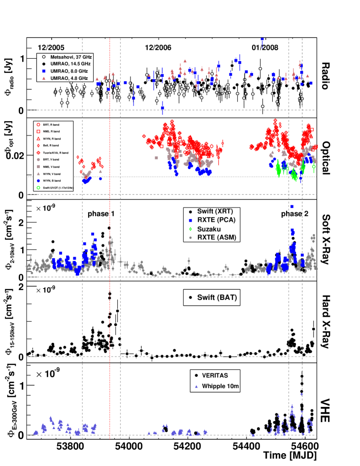
Figure 1: Mrk 421 light curves measured by different experiments (see Section 2) in 2006-2008. All errors are statistical errors only. Shown are the radio band (upper panel), the optical band (second panel), the X-ray band (third & fourth panel) and the TeV band (bottom). Some of the RXTE/ASM and Swift/BAT flux points have been re-binned for better visibility. Two phases of activity can be identified in the X-ray and TeV bands (phases 1 and 2). The vertical dotted line indicates the maximum of the hard X-ray flux (Swift/BAT, phase 1). During phase 2 a very good X-ray/TeV coverage was achieved, where the X-ray observations were partly triggered by VERITAS.

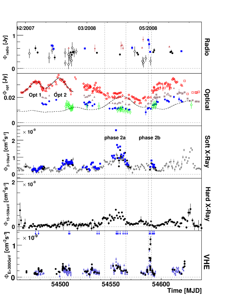
Figure 2: 2008 Mrk 421 light curves. For details see caption and legends in Figure 1. The vertical lines enclose phases of enhanced X-ray (phase 2a) and enhanced TeV (phase 2b) activity; see Figure 3 for a zoomed view of these phases. An exponential rise/fall function was fitted to the optical R band Tuorla/KVA data (’Opt 1’ & ’Opt 2’, see discussion in Sec. 3.4 and fit results in Tab. 3). The dashed line represents the optical rise/fall function folded with the ASM X-ray (dwell-by-dwell) light curve (see text for disussion). The vertical arrows pointing downwards in the bottom panel indicate the dates for which we compiled quasi-simultaneous SEDs and modeled them with a SSC code (see Figures 11 & 12).

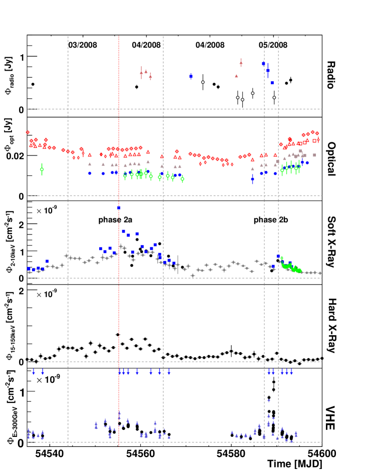
Figure 3: Mrk 421 light curves measured during the X-ray/TeV flaring state in April/May 2008 (phase 2). For details see caption and legends in Figure 1. The vertical dotted line highlights the brightest X-ray flare observed with the RXTE/PCA. The vertical arrows pointing downwards in the bottom panel indicate the dates for which we compiled quasi-simultaneous SEDs and modeled them with a SSC code (Figures 11 & 12).

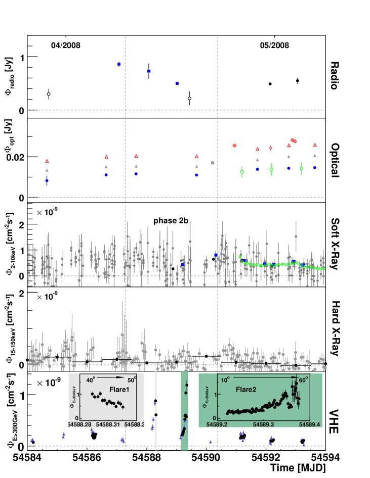
Figure 4: Mrk 421 light curves measured during the TeV flaring state in April/May 2008 (phase 2b). For details see caption and legends in Figure 1. Note, that the highest TeV flux around MJD 54590 was not accompanied by an increase in X-ray activity (compare with Figure 10). The continuous Suzaku/XIS soft X-ray monitoring (starting two days after the strong TeV flare) is shown, as well. The inserts in the lowest panel show the VERITAS TeV light curves in a $3\,\rm{min}$ binning, covering the flaring time span indicated by the colored, vertical boxes. The flares were recorded under mostly large zenith angles (indicated by the arrows) with a correspondingly higher systematic error on the flux, see text for more details.

3.2 Temporal and Spectral Variability in the TeV $\gamma$-Ray Band

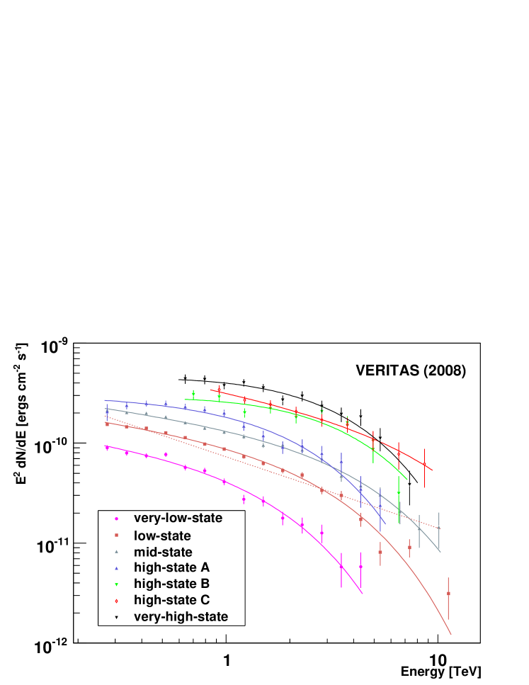
Figure 5: Time-averaged VERITAS energy spectra for different flux levels. Only data taken in 2008 are used. A power-law with exponential cutoff is fit to each spectrum (curves), the fit parameters and statistical errors are summarized in Table 2. The dotted line shows a power-law fit to the low-state spectrum to illustrate the incompatibility of this model and the data. The high-flux spectra were taken at zenith angles $z>35\deg$ with a correspondingly higher energy threshold.

Flux variability.

Flux variations on time scales of 1-2 days are found in the TeV band. Except for two nights measured during a strong flare in May 2008 (phase 2b, Figure 3), no significant TeV flux variations are observed within individual nights. It should however be mentioned, that the observation time during individual nights often did not exceed $10-20\,\rm{min}$. This prevents placing strong constraints on the $\gtrsim$0.5$-$1 h time scale variability, given the low/medium states of Mrk 421 during most of the measurements. Nevertheless, the strong outburst measured in May 2008 (Figure 4) clearly shows variability on sub-hour time scales even though the flare was recorded at zenith angles down to $60\,\deg$ (see inserts in Figure 4). At high zenith angles $z$, the effective areas vary drastically with a small change in $z$ and the sensitivity suffers from the strongly increased energy threshold (leading to a huge loss in event statistics). Since the data points in the light curve are given above $300\,\rm{GeV}$, the calculated fluxes (for the zenith angle range of $40\deg-60\deg$) are derived (extrapolated) based on the measured spectral shapes ($\rm{d}N/\rm{d}E=I_{0}\cdot(E/1\,\rm{TeV})^{-\Gamma}\cdot\exp(-E/E_{\rm{cut}})$). Therefore, an increased systematic error on the integral flux of $\sim$30$\%$ for $z>45\deg$ and $\sim$40$\%$ for $z>55\deg$ is assumed. Given these facts, we do not determine a quantitative value for the flux doubling times observed during this flare.

Spectral variability.

To investigate a possible change of the spectral shape as a function of flux state, the data are divided into subsets according to different flux levels. The separation into flux intervals is chosen such that reasonable statistics are guaranteed for each subset. An energy spectrum is derived (see Section 2.1) for each subset and is subsequently fit by a power-law function with exponential cutoff $\rm{d}N/\rm{d}E=I_{0}\cdot(E/1\,\rm{TeV})^{-\Gamma}\cdot\exp(-E/E_{\rm{cut}})$. A fit of a simple power-law function can be excluded with high confidence for most of the spectra (see as an example the dotted line in Fig. 5, resulting in a $\chi^{2}/\rm{dof}=264.3/15$). The results of the fits are summarized in Table 2 and the energy spectra are shown in Figure 5. No correlation between the cutoff energy $E_{\rm{cut}}$ and the flux normalization $I_{0}$ can be claimed. The spectra are also fitted with the same function by fixing the cut-off energy to $E_{\rm{cut}}=4\,\rm{TeV}$ (Table 2). In this case, a hardening of the spectrum with increasing flux level can be seen, see Figure 6. A linear correlation between the flux and the index $\Gamma$ is disfavored ($\chi^{2}/\rm{dof}=44.6/5$, $p=1.7\cdot 10^{-08}$) as compared to a quadratic relationship $\Gamma(I_{0})=a+b\cdot I_{0}+c\cdot I_{0}^{2}$ with $a=2.70\pm 0.04$, $b=(-5.3\pm 0.6)\cdot 10^{9}$ and $c=(1.08\pm 0.20)\cdot 10^{19}$ ($\chi^{2}/\rm{dof}=13.2/4$, $p=0.01$). This finding indicates that the spectral hardening with flux level flattens at very high flux values, as was seen already in the case of PKS 2155-304 (Aharonian et al., 2009b). Given the sparse sampling during most of the nights, we were not able to further separate the data into rising and falling (with time) flux states which may have an effect on the $\Gamma(I_{0})$ function. However, the general flux versus $\Gamma$ trend is in good agreement with earlier results obtained with the Whipple $10\,\rm{m}$ telescope (Krennrich et al., 2002) which are also shown in Figure 6.

Table 2: Parameters and statistical errors of fits $\rm{d}N/\rm{d}E=I_{0}\cdot(E/1\,\rm{TeV})^{-\Gamma}\cdot\exp(-E/E_{\rm{cut}})$ to the energy spectra shown in Figure 5: observation time $T_{\rm{live}}$, statistical significance of the excess in the data set, flux normalization $I_{0}$, photon index $\Gamma$, cut-off energy $E_{\rm{cut}}$ and the quality of the fit. The second row for each flux state corresponds to a fit in which the cut-off energy was fixed to a value of $E_{\rm{cut}}=4\,\rm{TeV}$.

	$T_{\rm{live}}[\rm{h}]$	$\rm{sign.}[\sigma]$	$I_{0}\,[\frac{10^{-11}}{\rm{cm}^{-2}\,\rm{s}^{-1}\,\rm{TeV}^{-1}}]$	$\Gamma$	$E_{\rm{cut}}\,[\rm{TeV}]$	$\chi^{2}/\rm{dof}$
very-low-state	$7.83$	$77.62$	$4.78\pm 0.73$	$2.29\pm 0.11$	$1.59\pm 0.34$	$17.8/11\,(1.62)$
			$3.056\pm 0.086$	$2.608\pm 0.033$	$4\pm 0$	$29.2/12\,(2.44)$
low-state	$16.3$	$181.3$	$7.60\pm 0.33$	$2.285\pm 0.035$	$2.95\pm 0.29$	$20.7/14\,(1.48)$
			$6.769\pm 0.084$	$2.375\pm 0.015$	$4\pm 0$	$29.3/15\,(1.95)$
mid-state	$7.79$	$160.6$	$10.26\pm 0.44$	$2.278\pm 0.037$	$4.36\pm 0.58$	$14.9/15\,(0.99)$
			$10.54\pm 0.15$	$2.256\pm 0.017$	$4\pm 0$	$15.4/16\,(0.96)$
high-state A	$1.38$	$73.0$	$19.08\pm 2.63$	$2.01\pm 0.12$	$1.91\pm 0.41$	$15.6/12\,(1.30)$
			$13.53\pm 0.38$	$2.295\pm 0.037$	$4\pm 0$	$24.0/13\,(1.84)$
high-state B	$0.63$	$47.3$	$22.23\pm 2.42$	$1.88\pm 0.24$	$3.06\pm 1.07$	$13.4/6\,(2.24)$
			$20.77\pm 1.14$	$2.053\pm 0.080$	$4\pm 0$	$143.0/7\,(2.00)$
high-state C	$0.63$	$53.76$	$21.74\pm 1.97$	$2.40\pm 0.26$	$9.6\pm 9.0$	$0.9/6\,(0.15)$
			$23.96\pm 1.62$	$2.05\pm 0.09$	$4\pm 0$	$2.7/7\,(0.39)$
very-high-state	$0.63$	$63.5$	$35.77\pm 3.08$	$1.87\pm 0.17$	$2.74\pm 0.60$	$6.2/9\,(0.69)$
			$32.0\pm 1.2$	$2.111\pm 0.057$	$4\pm 0$	$8.7/10\,(0.87)$

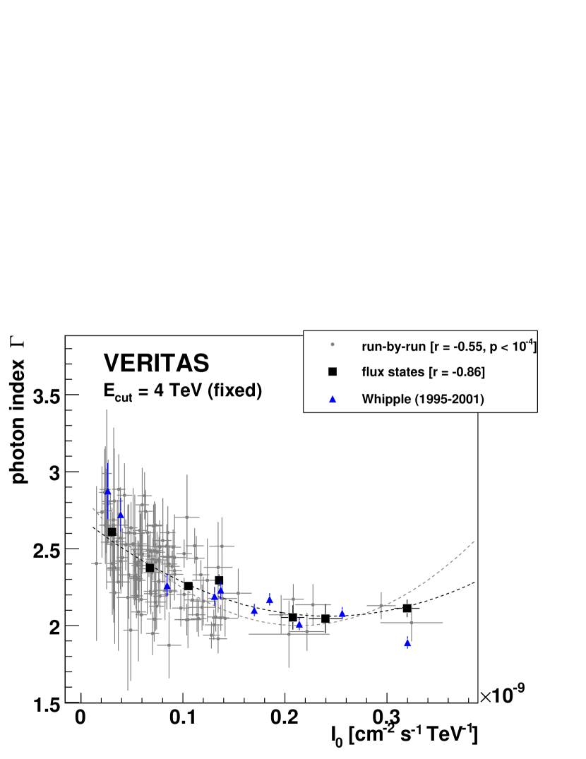
Figure 6: Photon index $\Gamma$ versus flux normalization $I_{0}$ (at $1\,\rm{TeV}$) obtained from a power-law fit with exponential cutoff (fixed to $E_{\rm{cut}}=4\,\rm{TeV}$, statistical errors only). Each gray data point corresponds to a data run with a duration of $10$ to $20\,\rm{min}$. The black points correspond to the values obtained from the fits to the spectra grouped according to their flux states (defined in Figure 5 and Table 2). Correlation coefficients $r$ and the corresponding chance probabilities for the null hypothesis (no correlation) are given in the legend. Results obtained from earlier Whipple 10m observations (Krennrich et al., 2002) are shown for reference.

Mrk 421 is detected by VERITAS (on average) with a statistical significance well above 10 standard deviations per run, even for runs with a duration of only 10 min. This enables a run-by-run derivation of the energy spectrum on time intervals of 10 min or less. Any energy spectrum derived from an individual data run which meets the following requirements is fit by a power-law with exponential cutoff (the cutoff energy again being fixed to $E_{\rm{cut}}=4\,\rm{TeV}$): (i) A differential flux point is only considered in a fit if the statistical significance of the excess is above 2 standard deviations; (ii) An energy spectrum is only fit if at least four differential flux points fulfill the first criterion. The results of the energy spectra derived for the individual runs are shown in Figure 6 (gray points) and confirm the trend which has been found already in the data sets divided according to the different flux levels. For both cases, the correlation coefficient was calculated and the corresponding non-directional chance probability for the null hypothesis $p$ (non-correlation) was calculated using the Student t-distribution. The correlation coefficients are $r=-0.86$ for the data sets separated by flux level, and $r=-0.55$ ($p<10^{-4}$) for the distribution based on the run-by-run data sets.

3.3 Temporal and Spectral Variability in the X-ray Band

Energy spectra and fluxes.

The RXTE/PCA spectra were fitted in an energy range of $3-20\,\rm{keV}$, while the Swift/XRT spectra were fitted between $0.4-10\,\rm{keV}$. Two models were tested to fit the data: a power law $\Phi(E)=kE^{-\Gamma}$ and a log-parabolic model $\Phi(E)=kE^{-(a+b\log(E/E_{0}))}$ (Massaro et al., 2004, 2006). The log-parabolic function uses an energy dependent photon index $\Gamma(E)=a+b\log(E/E_{0})$; the parameter $b$ defines the curvature in the logarithmic parabola, and $a$ is the spectral index at $E_{0}$. Both models account for absorption assuming a fixed galactic column density of $1.61\times 10^{20}\,\rm{cm}^{-2}$ (Lockman & Savage, 1995). The mean reduced $\chi^{2}$ values from log-parabolic fits to Swift/XRT and RXTE/PCA data are $1.20$ ($96$ dof) and $0.87$ ($161$ dof), respectively. These are significantly lower than the respective mean reduced $\chi^{2}$ values from power law fits of 1.80 and 1.35. Hence, the integral flux from $2-10\,\rm{keV}$ was calculated for each observation from log parabolic fits.

Flux variability and light curves.

The X-ray light curves of the $2-10\,\rm{keV}$ fluxes are shown in Figures 1 to 4. Significant day time-scale flaring is seen in many months in both 2006 and 2008, while for the observations in 2007 the Mrk 421 X-ray flux remained relatively low. Of particular interest are the observations in March to May 2008. RXTE/PCA recorded one of the highest ever X-ray fluxes for Mrk 421 on March 30, 2008 (phase 2a). However, during the very high TeV $\gamma$-ray flux state measured by VERITAS in early May 2008 (phase 2b) the near-simultaneous X-ray flux was only found to be at a moderate level. For all but one case the RXTE observation exposures were shorter than 1.5 hours (with an average exposure of $25\,\rm{min}$). The Swift observations had a far larger range in exposures, from 15 minutes in many observations, to over 40 hours in each of seven observations; the average exposure per pointing was $3.3\,\rm{hrs}$. Significant variability in both RXTE/PCA and Swift/XRT observations was found. The corresponding Swift observations spanned up to 3 days, with clear flaring in the rates on hour time-scales. Some of the RXTE/PCA light curves show a steady change in the count rate over 20 minute periods. However, more detailed studies of the sub-day flux variations in the X-ray data are beyond the scope of this paper.

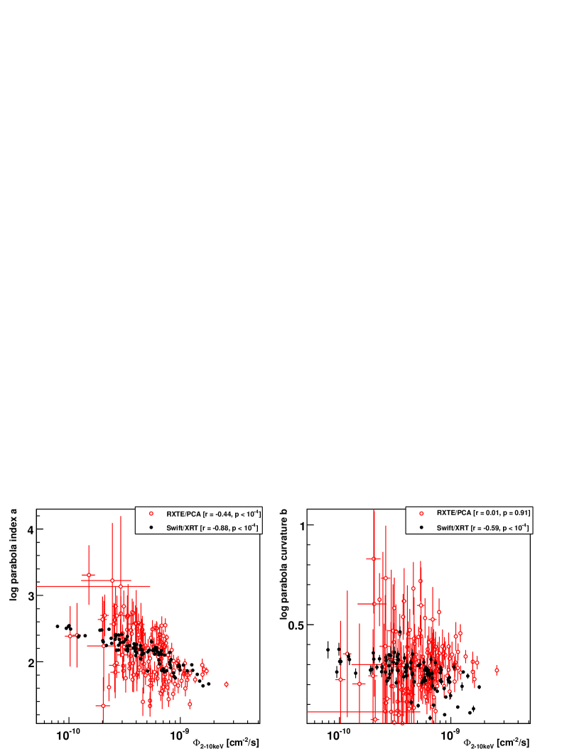
Figure 7: Correlations between the spectral shape and the flux level for the X-ray data sets taken with RXTE/PCA and Swift/XRT. Correlation coefficients $r$ and the corresponding chance probability for the null hypothesis (no correlation) are given in the legends. Left: The log-parabola parameter $a$ vs. the $2-10\,\rm{keV}$ photon flux. Right: The log-parabola curvature parameter $b$ vs. the $2-10\,\rm{keV}$ photon flux.

Spectral variability.

Drawing from this large set of X-ray observations, the correlation of X-ray flux to spectral shape is investigated here. This will allow identification of trends which could give important input to the modeling. The left panel of Figure 7 shows the correlation plot between the log-parabola parameters $a$ (index) vs. the $2-10\,\rm{keV}$ flux. The corresponding correlation plot between the curvature parameter $b$ and the flux is shown in the right panel of Figure 7. Although the index $a$ is not independent of the curvature parameter $b$, the conclusion can be reached that an increased flux is accompanied by a hardening of the spectrum (parameter $a$) since there is only a moderate correlation between the flux and $b$. This finding is compatible with earlier findings (Fidelis & Iakubovskyi, 2008). The (anti)correlation between $a$ and the flux is significant: the non-directional chance probability of the derived correlation coefficient for the null-hypothesis is $p<10^{-4}$ for the RXTE/PCA data, as well as for the Swift/XRT data.

3.4 Flux Correlation Analysis

This section describes the search for flux correlations between the light curves measured in different energy bands and is based on the light curves shown in Figures 1 to 4.

Radio/optical/TeV flux correlations.

Table 3: Parameters of an exponential rise/fall function (Sec. 3.4) $\Phi_{\rm{opt}}(t)=a+b/(e^{-(t-T_{0})/\tau_{\rm{r}}}+e^{(t-T_{0})/\tau_{\rm{f}}})$ fitted to the optical flares ’Opt 1’ and ’Opt 2’ (Fig. 2).

Parameter	Opt 1	Opt 2
$a$ [Jy]	$0.021\pm 0.001$	$0.023\pm 0.001$
$b$ [Jy]	$0.023\pm 0.002$	$0.024\pm 0.003$
$\tau_{\rm{r}}$ [d]	$7.16\pm 1.78$	$9.52\pm 1.35$
$\tau_{\rm{f}}$ [d]	$5.46\pm 0.80$	$4.46\pm 0.77$
$T_{0}$ [MJD]	$54476.8\pm 1.4$	$54501.4\pm 0.7$

As can be seen in Figure 1 there is no significant variation in the radio flux on day, week, or month time scales. Thus, no significant correlation with fluxes measured in the other wave bands is found. This could be explained if (i) the dominant portion of the radio emission does not originate from the inner jet region that likely produces the flux variability in the other energy bands, or (ii) structures in the light curve are smeared out due to slower cooling of the radio emitting electrons compared to the electrons responsible for the shorter wavelength emission (see Sec. 4). The optical fluxes, on the other hand, show clear variability on time scales of weeks (Figure 2), where the fluxes from the different bands (R, B, and V) are clearly correlated. This is not surprising since the frequency filter bands are not largely separated in terms of photon energy and a common origin of the radiation in the three bands can be assumed. Figure 8 shows the correlation plot between the VERITAS TeV $\gamma$-ray fluxes and the optical fluxes in the R, B, and V bands. A maximum time gap between the TeV and optical measurements of $\Delta t\leq 0.5\,\rm{days}$ was allowed for the individual data pairs. The corresponding correlation factors are compatible with chance expectations. A similar correlation study between X-ray and optical fluxes did not result in any significant correlation coefficient, either. Given the different time scales of the flux variations (sub-day level in the X-ray and TeV band, and weeks in the optical band), the lack of a direct flux correlation is expected.

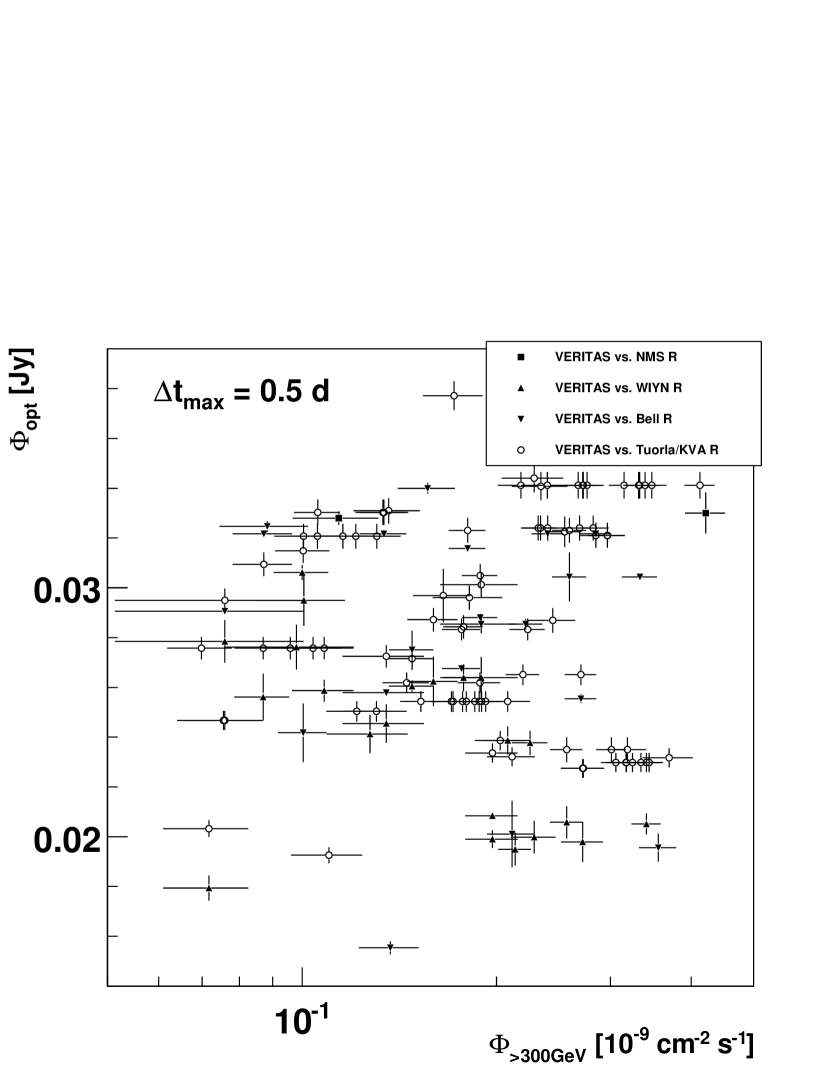
Figure 8: Correlation between TeV and optical fluxes. The maximum allowed time difference between the data points is $\Delta t\leq 0.5\,\rm{days}$.

Except for the Swift/UVOT data the contribution of the host galaxy is not subtracted. Since it has to be constant in time, the light curves can be used to set an upper limit on the base-line, which in turn would be an upper limit on the host galaxy contribution in the measured data. This contribution is estimated to be $0.009\,\rm{Jy}$ (R band, see dotted line in Fig. 1), $0.009\,\rm{Jy}$ (V band), and $0.006\,\rm{Jy}$ (B band). These estimates are somewhat lower as compared the modeling of Nilsson et al. (1999) who estimate $0.014\,\rm{Jy}$ for the R band. Although neither instantaneous nor delayed correlation between the optical and the X-ray/TeV bands was found it is important to study the structure of the optical light curves. Two well defined flares ’Opt 1’ and ’Opt 2’ (Figure 2) were fitted with an exponential rise/fall function $\Phi_{\rm{opt}}(t)=a+b/(\exp(-\frac{t-T_{0}}{\tau_{\rm{r}}})+\exp(\frac{t-T_{0}}{\tau_{\rm{f}}}))$. The fit parameters are summarized in Tab. 3, showing that the optical flux changes on time scales of less than ten days with the indication of slightly shorter fall times $\tau_{\rm{f}}$ as compared to the rise times $\tau_{\rm{r}}$. These time scales are on the same order as the estimated value of $\sim$$15\,\rm{d}$, based on the characteristic X-ray/TeV variability time scale of $\leq 0.5\,\rm{d}$ (see the discussion in Sec. 4). One can interpret $\Phi_{\rm{opt}}(t)$ as a ’characteristic’ optical response to a single X-ray/TeV flare. With this assumption a hypothetical prediction can be made for the optical light curve by folding $\Phi_{\rm{opt}}(t)$ (using $\tau_{\rm{r}}=7\,\rm{d}$ and $\tau_{\rm{f}}=5\,\rm{d}$, and a delay $\Delta T=7\,\rm{d}$) with the X-ray and/or TeV $\gamma$-ray light curves. The prediction based on the frequently sampled RXTE/ASM X-ray light curve (dwell-by-dwell, MJD $54450$ to $54630$, linear interpolation between the flux points) is shown together with the optical light curve in Figure 2 (arbitrary units) – no agreement is found. A caveat should be mentioned: the RXTE/ASM flux measurements are not very accurate; however, the general trends (high- vs. low-state) should allow the comparison of the two different wave bands. $\Phi_{\rm{opt}}(t)$ was also folded with the TeV $\gamma$-ray light curve (MJD $54500$ to $54630$, linear interpolation between the flux points). Again, no correlation can be found. There is a caveat here, as well: the non-continuous sampling of the TeV $\gamma$-ray light curve and the short duty-cycle of flares results in a considerable chance that one or more strong $\gamma$-ray flares have been missed which would change the shape of the folded optical light curve. Therefore, the latter results are not shown in Figure 2. Furthermore, our above comparison ignores the possibility that particles with different energies are injected at the beginning of the flare.

Hard/soft X-ray flux correlations.

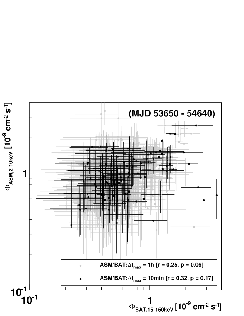
Figure 9: Hard/soft X-ray flux correlation between the $15-150\,\rm{keV}$ Swift/BAT flux and the $2-10\,\rm{keV}$ RXTE/ASM flux. All dwell-by-dwell flux points with a statistical significance above $2\,\sigma$ measured in the first half of 2008 (MJD 54457–54640) are shown for two cases of a maximum time lag between the observed data points. The legend gives the corresponding correlation coefficient and the corresponding chance probability for the non-correlation.

The correlation between hard and soft X-ray fluxes is studied based on the dwell-by-dwell flux points measured with Swift/BAT ($15-150\,\rm{keV}$) and RXTE/ASM ($2-10\,\rm{keV}$). The correlation plot including all data points taken in spring 2008 (MJD 54457–54640, contemporaneous with the VERITAS coverage) with a statistical significance of more than $2$ standard deviations is shown in Figure 9. The distribution was generated for two different requirements regarding the maximum allowed time gap between the center time of the individual pointings ($\Delta t\leq 1\,\rm{h}$ and $\Delta t\leq 10\,\rm{min}$). In both cases, indications for only a weak correlation of $r\simeq 0.1$ are found with moderate significance. However, while the RXTE/ASM data are testing the falling edge of the synchrotron peak in the SED, the Swift/BAT data likely fall into the transition zone between synchrotron and high-energy peaks, compare with Figures 11 and 12.

X-ray/TeV flux correlations.

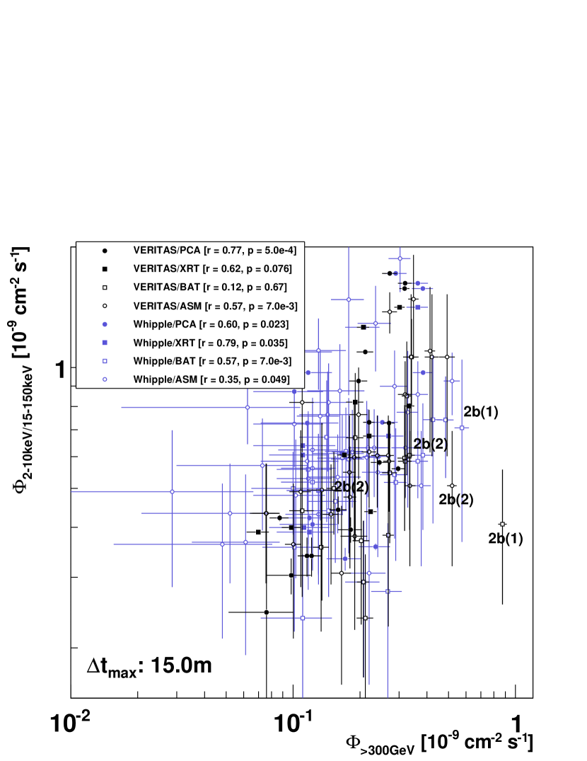
Figure 10: Correlation between TeV fluxes (VERITAS and Whipple) and X-ray fluxes (RXTE: PCA & ASM, Swift: XRT & BAT). All X-ray fluxes are given between $2-10\,\rm{keV}$, except for the Swift/BAT fluxes which are given between $15-150\,\rm{keV}$. Only data measured in the first half of 2008 (MJD 54457–54640) are shown. The RXTE/ASM and Swift/BAT fluxes are dwell-by-dwell with the requirement that the statistical significance is above $2$ standard deviations. The maximum time difference between the data points is $\Delta t\leq 15\,\rm{min}$. The correlation coefficients including the chance probability for the null hypothesis are shown in the legend. The flux pairs measured during the first (2b(1)) and second night (2b(2)) of phase 2b are marked.

The rich data sets allow for a detailed study of the X-ray versus TeV flux correlations. The TeV runs have a duration of $10-20\,\rm{min}$. With a few exceptions (during the highest flare) no indications for TeV flux variations were found within any of the runs. A maximum time lag between the correlated X-ray/TeV data points of $\Delta t\leq 15\,\rm{min}$ was allowed (close to the average TeV run duration). Since some of the dedicated, high-quality data from Swift/XRT and RXTE/PCA were considerably longer in exposure, an additional cut on the total length of the X-ray pointing was applied (based on the average exposure per pointing): $\Delta T\leq 30\,\rm{min}$ in the case of RXTE/PCA and $\Delta T\leq 2\,\rm{h}$ in the case of Swift/XRT. Flux variations within individual X-ray pointings are not investigated in the framework of this paper; therefore, the data pairs cannot be considered as exactly simultaneous. The RXTE/ASM and Swift/BAT dwell-by-dwell data points have exposures of the order of $1-10\,\rm{min}$, so that no cut on $\Delta T$ was applied in those cases. Individual RXTE/ASM and Swift/BAT flux measurements were only considered in case of a significance level of $\geq 2\,\sigma$. The results discussed below do not strongly depend on the exact choice of $\Delta t$ and $\Delta T$. Figure 10 shows the flux correlations for the data taken in spring 2008 (MJD 54457–54640). The correlation coefficients and the corresponding non-directional chance probability for the null hypothesis (no correlation) were calculated and are shown in the figure legend. The X-ray and TeV fluxes seem to be correlated ($r>0.5$ for most data subsets) with chance probabilities of the order of a few percent or below. The VERITAS/BAT data set is the only one which is not correlated in a significant manner. One of the high TeV flux points measured during the strong TeV $\gamma$-ray flare (Figure 4) was accompanied by a Swift/BAT dwell-by-dwell pointing ($\Delta t\leq 3.4\,\rm{min}$), which however did not indicate an increased activity in the hard X-ray band. The Swift/BAT point has a duration of $8\,\rm{min}$ and is therefore fully contained in the time intervall of the corresponding VERITAS data run of $20\,\rm{min}$ duration. This flux pair is located in the lower right corner of Figure 10 (labeled as 2b(1)) and may be seen as the indication of an orphan TeV $\gamma$-ray flare. However, since this indication is based on only one X-ray/TeV flux pair measured during a high TeV $\gamma$-ray flux state, there is not enough evidence for a strong claim. If the corresponding data pair were removed, the VERITAS/BAT flux correlation would increase to $r=0.62$ with a chance probability of $p=0.019$. Other flux pairs from the two TeV flare nights (phase 2b) are indicated in Figure 10, as well.

Discrete correlation functions.

The light curves were also analyzed using the discrete correlation function (DCF) technique (Edelson & Krolik, 1988) in order to search for correlated/delayed emission between different energy bands, allowing for significant time lags (i.e. one light curve having the delayed shape of another one). The radio, optical and X-ray light curves were tested against the TeV $\gamma$-ray light curve. Except for the zero lag X-ray/TeV correlation (see above) no significant time lag and/or correlation at zero time lag was found for the radio and optical band as compared to the TeV $\gamma$-ray emission.

3.5 Spectral Energy Distributions and Modeling

The spectral energy distributions (SEDs) showing the VERITAS and multi-wavelength (MWL) data were generated for individual nights and plotted in Figures 11 and 12. Based on the different variability time scales, data from the different wavebands are plotted in the quasi-simultaneous SEDs if the time lag $\Delta t$ between the MWL data and the TeV data is $\Delta t_{\rm{X-ray}}\leq 0.15\,\rm{d}$ (X-ray), $\Delta t_{\rm{opt}}\leq 1.5\,\rm{d}$ (optical), and $\Delta t_{\rm{radio}}\leq 3\,\rm{d}$ (radio). Shorter time lags are present (down to real simultaneity) and the exact times are given in the figure legends of the SEDs. The time spans (duration) of the X-ray observations are given in the legends, as well. Possible spectral variations within individual X-ray observations are beyond the scope of this paper and are ignored in the modeling of the SEDs. The X-ray spectra (Swift/XRT and RXTE/PCA) were fit with a log-parabola model $\Phi(E)=kE^{-(a+b\log(E))}$, and the corresponding log-parabola bow ties including the statistical errors of the fits are shown if the fit resulted in a $\chi^{2}/\rm{dof}<2$. All errors are statistical only. As a reference, Figures 11 and 12 also show the non-simultaneous MeV/GeV energy spectrum measured by the Fermi/LAT (Atwood et al., 2009) in August 2008, to July 2009 (Abdo et al., 2010). During this period, the LAT detects Mrk 421 with a statistical significance of $88\,\sigma$ and the energy spectrum is well fit by a power law in the whole energy range (curvature index given in the Fermi catalog of $0.72$). Interestingly, the variability index of $43.9$ does not indicate very strong variability during the above period, so that the Fermi/LAT energy spectrum shown in the SEDs may give a realistic indication for a low/medium flux state of Mrk 421. However, given the non-simultaneity of the Fermi observations, the MeV/GeV spectrum was not included in the modeling. The SEDs were fit with a one-zone SSC model following Krawczynski et al. (2004). In this model a spherical emission region of radius $R$ is filled with a relativistic electron population, traveling down the jet with a bulk Lorentz factor $\Gamma$ ($\beta=v/c$). The magnetic field $B$ in the emission region is randomly oriented. The emitted radiation is Doppler-shifted by $\delta=[\Gamma(1-\beta\cos\theta)]^{-1}$, $\theta$ being the angle between the jet axis and the line of sight of the observer. The electron distribution is normalized by a factor $u_{\rm{e}}$ (in units of ergs/cm³) and is described in the jet frame by a broken power law with $E_{\rm{min}}$, $E_{\rm{brk}}$, and $E_{\rm{max}}$ and the two corresponding spectral indexes $\alpha_{1}=-2.2$ and $\alpha_{2}=-3.2$. Mrk 421 is located at a redshift of $0.031$ so that the energy-dependent pair absorption on photons of the extragalactic background light (EBL) cannot be neglected. EBL absorption is taken into account in the model following Franceschini et al. (2008). Since most of the optical data were not corrected for the contribution of the host galaxy, the optical data points have to be seen as an upper limit on the jet emission region. The estimate on the host galaxy contribution (Sec. 3.4) has been added as a systematic error. The SSC model was adjusted to the SEDs with the following procedure:

• In a first step, the three SEDs with the smallest time lags between the X-ray and the TeV spectra (MJD 54559.25, 54562.25, and 54509.37) were used to derive a full set of model parameters. The Doppler factor was set to $\delta=40$ and the magnetic field was set to $B=0.2\,\rm{G}$, in agreement (order of magnitude) with a synchrotron cooling time of $\tau_{\rm{sync}}(B)\times\delta\,\approx$ $T_{\rm{flare}}\,=1\,\rm{h}$ for the electrons emitting the synchrotron emission close to the maximum of the spectral energy distribution. Then, the radius $R$, the energy density in electrons $u_{\rm{e}}$ [ergs/cm³], as well as $E_{\rm{brk}}$ and $E_{\rm{max}}$ were varied until the model would describe the SED (optical to TeV).

• In a second step, the remaining SEDs were fit by only allowing variations of $u_{\rm{e}}$ and $E_{\rm{max}}$ (and in case of bad fits also $E_{\rm{brk}}$) as compared to the model parameters derived above, reflecting a change in the injected electron population.

The SSC model fits are shown in Figure 11 and 12 and the model parameters for the individual SEDs are summarized in Table 4. The models generally under-predict the radio emission which is synchrotron self-absorbed in the model at the low-energy tail of the SED. This discrepancy could be explained by additional radio emission from regions in the jet not emitting the TeV radiation. Also, the synchrotron self-absorbed radio blobs could expand and lead to a delayed radio emission from a larger region (Acciari et al., 2009a), which however is not taken into account in the model. The break energy $E_{\rm{brk}}$ of the electron spectrum is very near the maximum energy of the electron spectrum $E_{\rm{max}}$. The missing plateau ($E_{\rm{brk}}\sim E_{\rm{max}}$) is directly seen in the Swift/XRT data which show a direct turn-over of the synchrotron peak. This is in agreement with earlier findings in the case of Mrk 421 (Fossati et al., 2008) and is in contrast to the SEDs measured in the case of Mrk 501 for which the synchrotron emission peaks at higher energies and shows indications of a plateau (Krawczynski et al., 2000). If $E_{\rm{min}}\ll E_{\rm{brk}}$, the missing plateau implies that cooling did not have time to kick in. However, if $E_{\rm{min}}=E_{\rm{brk}}$ and cooling is very efficient, electrons cool below $E_{\rm{brk}}$ and one gets a new ’effective’ $E_{\rm{min}}\ll E_{\rm{brk}}$, and the ’true’ $E_{\rm{min}}$ becomes $E_{\rm{brk}}$. All SEDs are reasonably described by using the same model parameters except for the electron normalization $u_{\rm{e}}$ and the break/maximum electron energies $E_{\rm{brk}}$ and $E_{\rm{max}}$ which were adjusted for each individual SED (Table 4). The only exceptions are the X-ray flare (Figure 11) and the two TeV $\gamma$-ray flare SEDs (Figure 12):

• MJD 54555.38: The RXTE/PCA bowtie shown in this SED (Figure 11) does not qualify for the previously defined X-ray/TeV time lag criterion. However, the X-ray flux is the highest one measured during the whole MWL campaign (see dotted line in Figure 3) so that it is shown for reference (but not included in the fit). The closest Whipple TeV flux point is $\sim$$2\,\rm{h}$ away and also does not show signs for an increased TeV flux. This may indicate an orphan X-ray flare, but the lack of simultaneous TeV data does not allow a strong conclusion.

• MJD 54588.3: The SSC model slightly over-predicts the optical emission. However, the optical data are not simultaneous and the TeV fluxes can change within $20\,\rm{min}$: the black data points in Figure 12 represent the first $20\,\rm{min}$ of the flare, whereas the open gray points represent the second $20\,\rm{min}$ of the flare in that night (compare with the lower left insert in Figure 4). Unfortunately, no X-ray data (Swift/XRT or RXTE/PCA) were taken during this night.

• MJD 54589.21: The black data points in Figure 12 represent the low plateau at the beginning of the flare – compare with the lower right insert in Figure 4 – and are the ones which were used for the fit of the SED. The RXTE/PCA measurement partially overlapped this time, but is over-predicted by the model. Given the generally good fits of the model, this is interesting since the VERITAS/BAT flux pairs of the same night (see 2b(2) in Figure 10) as well as the previous night (2b(1)) also indicate a possible orphan TeV $\gamma$-ray flare. The higher flux states during this flare night (open gray points in Figure 12) were not accompanied by simultaneous X-ray measurements and were therefore not modeled.

The fact that the X-ray (and optical) data are not perfectly described during the flare nights (as well as for a few other nights) may be explained by the fact that only $u_{\rm{e}}$, $E_{\rm{brk}}$ and $E_{\rm{max}}$ were allowed to vary, after the other parameters had been fixed based on the three most complete and contemporaneous SEDs, which all correspond to TeV low/medium states of Mrk 421.

Table 4: Parameters of the SSC models as shown in Figure 11 and 12. The following parameters are the same for all models: Doppler factor $\delta=40$, magnetic field $B=2.0\times 10^{-5}\,\rm{T}=0.2\,\rm{G}$, radius $R=2.5\times 10^{15}\,\rm{cm}$, $\log(E_{\rm{min}})=3.0$. The table shows the remaining parameters $u_{\rm{e}}$, $\log(E_{\rm{max}})$ and $\log(E_{\rm{brk}})$ for the different SEDs, as well as the particle energy density to magnetic field energy density ratio $u_{\rm{e}}/u_{\rm{B}}=8\pi u_{\rm{e}}/B^{2}$.

date	$u_{\rm{e}}$	$\log(E_{\rm{max}})$	$\log(E_{\rm{brk}})$	$u_{\rm{e}}/u_{\rm{B}}$
[MJD]	[ergs/cm3]
54475.4	0.45	10.8	10.5	283
54478.4	0.65	10.9	10.4	408
54508.3	0.50	11.0	10.6	314
54509.3	0.60	11.1	10.5	377
54536.4	0.40	11.0	10.6	251
54538.4	0.35	10.9	10.6	220
54555.4	0.40	11.2	11.2	251
54556.3	0.35	11.2	11.1	220
54557.3	0.40	11.3	11.0	251
54559.2	0.40	11.4	10.8	251
54562.2	0.40	11.3	10.6	251
54564.2	0.40	11.4	10.7	251
54566.2	0.40	11.2	10.6	251
54588.3	0.55	11.6	11.0	345
54589.3	0.43	11.5	10.6	270
54591.3	0.48	11.2	10.5	301
54592.3	0.35	11.0	10.6	220
54593.3	0.35	11.0	10.6	220

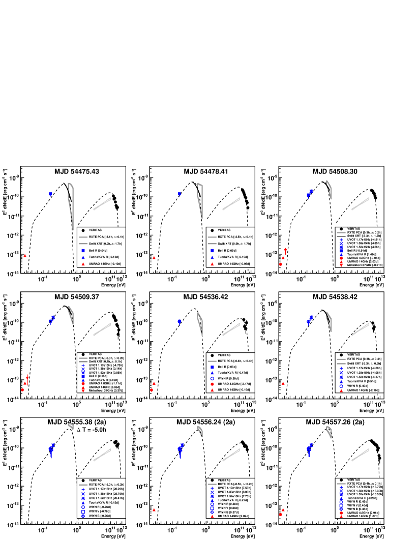
Figure 11: SEDs of Mrk 421 for individual dates showing all available MWL data (statistical errors only) if the corresponding time lag criterion is met (see text for more detail). The legends indicate the time lags $\Delta T=T_{\rm{MWL}}-T_{\rm{TeV}}$ between the individual MWL data and the VERITAS data. For the X-ray observations, the duration of the pointing $\Delta$ is given, as well. The number in parentheses refers to the phase (2a or 2b) during which the The SEDs were fit by a one-zone SSC model (dashed curves); the corresponding model parameters are summarized in Table 4. The non-simultaneous MeV/GeV spectrum measured by Fermi (August 2008 to July 2009) is shown for reference (Abdo et al., 2010).

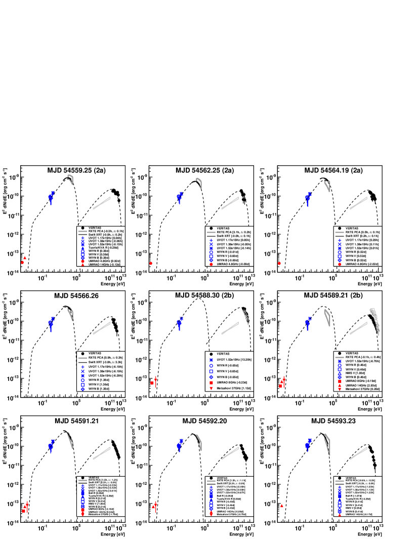
Figure 12: SEDs of Mrk 421, continued from figure 11. The SEDs of the two flare nights are also shown: MJD 54588.30 (no X-ray coverage in this night) and MJD 54589.21 with X-ray coverage during the onset of the flare (solid TeV points) but not during the high flare state (open TeV data points).

4 Summary and Discussion

Together with many MWL partners VERITAS conducted an intensive MWL campaign on Mrk 421 in 2008. During low states of Mrk 421, VERITAS is able to measure the source flux to an accuracy of $5\%$ in $20\,\rm{min}$ time intervals. In the $47\,\rm{hr}$ data set presented in this paper, we did not find evidence for rapid flux variability on time scales of minutes as reported for Mrk 501 (Albert et al., 2007) and PKS 2155-304 (Aharonian et al., 2009b). However, the only strong outburst (reaching a flux level of 10 Crab) which would have allowed testing these short time scales of flux variations was measured at high zenith angles with a strongly reduced detection sensitivity. Two phases of enhanced X-ray (phase 1) and X-ray/TeV (phase 2) activity are found. Phase 2 can be separated into a period of strong X-ray activity without a strong TeV $\gamma$-ray flaring, followed by a TeV $\gamma$-ray flare lasting for two days without any indication for contemporaneous strong X-ray activity. This may indicate an X-ray (phase 2a) and TeV $\gamma$-ray (phase 2b) orphan flare, but the data are too sparse for a definite claim. In the remaining data there is significant evidence for a correlation between the X-ray and TeV fluxes. No significant flux correlations between the TeV band and the optical/radio bands were found. Assuming that (i) the optical and X-ray/TeV photons are emitted co-spatially, and that (ii) the flux variability time scale equals the radiative cooling time, one can estimate the expected relation between the observed time scales of flux variations: The mean energy of emitted photons $E_{\rm{obs}}$ scales with the electrons’ Lorentz factor squared, $E_{\rm{obs}}\propto\gamma^{2}$. The cooling time $\tau_{\rm{cool}}$ scales proportional to $1/\gamma$. The energy of the X-ray photons is three orders of magnitude higher than the energy of the optical photons. The Lorentz factors of the X-ray emitting electrons should thus be $1.5$ order of magnitudes (factor $\sim$$30$) larger than the Lorentz factors of the optically emitting electrons. If the X-rays (and $\gamma$-rays, from inverse Compton scatterings of the electrons which emit X-rays as synchrotron emission) show flux variability on a time scale of $\leq 0.5\,\rm{d}$ (Fidelis & Iakubovskyi, 2008; Gaidos et al., 1996), then the optical fluxes should vary on a time scale of $\leq 15\,\rm{d}$ which is well compatible with the observed time scales in the optical and X-ray/TeV bands (Sec. 3.4). However, as discussed in Sec. 3.4, the optical light curve does not seem to be a delayed and stretched version of the X-ray light curve or the TeV $\gamma$-ray light curve, implying, that the dominant fraction of the observed optical emission does not originate from the X-ray/TeV emission region. Iterestingly, Rieger (2004) discusses variable (even periodic) flux variations on (periodic) time scales of $P\leq 10\,\rm{d}$ which can be explained by geometrical arguments of internal jet rotation. Our data, however, seems to indicate more complicated structures than periodicity. A similar estimate using the radiative cooling time for the energies in the radio band leads to time scales of $10$ years or more, impossible to test with the given MWL data set. Clear indications for spectral hardening with increasing flux levels are found in the X-ray and TeV bands. In the TeV band, the spectral hardening seems to level out for the very high fluxes above $\sim$5 Crab. A similar trend had already been found in earlier Whipple data of Mrk 421, as well as in the strong flare of PKS 2155-304 measured by H.E.S.S. (Aharonian et al., 2009b). The rich MWL data set presented in this paper allowed for the compilation of $18$ quasi-simultaneous SEDs, well constrained by accurate Swift/XRT X-ray and VERITAS TeV spectra. The SEDs can be described by a one-zone SSC model with nearly one set of parameters; only $u_{\rm{e}}$, $E_{\rm{brk}}$ and $E_{\rm{max}}$ needed to be adjusted to describe the whole set of SEDs. However, for most of the SEDs Mrk 421 was found to be in low or moderate flux states, leading to similar SEDs on different days. Our SSC modeling indicates that the emission process and the jet parameters are reasonably well constrained. So far, there are only four TeV blazars with a reasonable amount of simultaneous MWL data in order to claim a correlation between X-ray and TeV $\gamma$-ray fluxes: Mrk 421 (Fossati et al., 2008; Błażejowski et al., 2005; Horan et al., 2009), Mrk 501 (Krawczynski et al., 2002), PKS 2155-304 (Aharonian et al., 2009b), and 1ES 2344+512 (Acciari et al., 2010). Such a correlation implies that the same high-energy particle population (e.g. electrons) is responsible for the synchrotron emission at X-ray energies, as well as the high-energy IC emission at TeV energies, as predicted in the framework of SSC models. Investigating the exact shape of the X-ray/TeV correlation (linear, quadratic, etc.) will be one of the important goals for future studies. Although this correlation is seen as a general trend, it does not necessarily hold true at the level of individual flares (Krawczynski et al., 2004). In our data, we find indications of an X-ray high-state not accompanied by TeV $\gamma$-ray flaring (phase 2a), as well as a TeV $\gamma$-ray flare without increased X-ray activity (phase 2b). Although the data is not exactly contemporaneous – not allowing for a firm conclusion – such orphan flares in general would require fine tuning of the SSC model (Krawczynski et al., 2004) or alternative models, e.g. external-Compton models or models where the $\gamma$-ray emission is produced by hadrons, e.g. as proton-synchrotron emission (Mücke & Protheroe, 2001; Aharonian, 2002) or through a proton induced cascade (Mannheim, 1998). Further observations are needed to understand this particular aspect of the TeV flaring activity. Acciari et al. (2009b) reported comparable $\sim$week-scale trends between the Mrk 421 X-ray and optical fluxes without a strong X-ray/TeV coupling. Aharonian et al. (2009a) reported a clear indication of an optical/TeV flux correlation in case of PKS 2155-304. However, in the second PKS 2155-304 flare the optical/TeV correlation was not seen although the data were again strictly simultaneous (Aharonian et al., 2009b). Also, an optical/TeV correlation is not found in the large data sample presented in this paper or in earlier large data sets. Therefore, it does not seem to be a general property of TeV blazars. This may indicate that (part of) the optical emission is dominated by a region larger than the TeV emission site and/or a different emission mechanism is at play. However, a certain level of optical synchrotron emission is un-avoidable given the synchrotron emission at X-ray energies. The ambiguous findings so far in terms of the optical/TeV correlation may further indicate that different emission scenarios may play a role in different situations, e.g. we do not always observe the same type of flares. No correlation between TeV and radio fluxes has been established at this point resulting in similar arguments as above concerning the emission regions/mechanisms. TeV flux variations are measured for different TeV blazars with characteristic time scales down to $5-20\,\rm{min}$ (Albert et al., 2007; Aharonian et al., 2009b; Gaidos et al., 1996). Interestingly, the corresponding size of the emission region reaches down to the order of the Schwarzschild radius of the black hole of the corresponding AGN (Albert et al., 2007; Aharonian et al., 2009b). This can be seen as an indication that the TeV $\gamma$-ray emission from blazars comes from the base of the jet where the jet energy density is highest and the jet cross section is smallest. A similar finding was made in case of the radio galaxy M 87 for which a promising approach to locate the site of the TeV emission region was presented based on the combination of TeV $\gamma$-ray observations with simultaneous high-resolution radio observations (Acciari et al., 2009a). We see two paths towards improving our understanding of the inner workings of AGN jets. The first path involves simultaneous TeV observations with imaging telescopes with $\leq 1\,\rm{mas}$ angular resolution, e.g. VLBA (Acciari et al., 2009a), and/or with polarimetric observations in the optical (Marscher et al., 2008) and the X-ray band. Furthermore, future observations in the MeV/GeV band with Fermi, together with observations in the GeV/TeV band with VERITAS, will facilitate the study of the spectral slope, time scales and correlation of the fluxes in both energy bands which are important inputs for the theoretical modeling. The second path for achieving further progress concerns the theoretical modeling of the results. The analysis presented in this paper confirms that SSC models are successful in describing the broad-band spectral energy distributions of high-frequency peaked BL Lac objects. The two lessons which we infer from the modeling are (i) a large value of the relativistic Doppler factor $\delta$ is required to explain the SEDs and the rapid flux variability (Gaidos et al., 1996; Begelman et al., 2008); (ii) in the case of SSC models, the electron energy density exceeds the magnetic field energy density both measured in the rest frame of the emitting volume (see Table 4). In the case of EC models, one can find models with approximately equal electron and magnetic field energy densities (e.g. Ghisellini & Tavecchio (2009)), or models in which this ratio deviates considerably from unity Krawczynski et al. (2002). Considering that protons may add to the particle energy density, the particle energy density may still be an equally comparable component in the plasma blobs producing HBL flares. Further progress can be achieved by combining them with those from theories describing the formation and structure of jets. Recently, general relativistic magneto-hydrodynamic simulation codes (e.g. McKinney (2006); Komissarov (2007); Krolik & Hawley (2010); Spruit (2010)) have been used to validate aspects of analytic models of the magnetic formation, acceleration, and collimation of jets (Weber & Davis, 1967; Blandford & Znajek, 1977; Phinney, 1983; Camenzind, 1986; Lovelace, Wang & Sulkanen, 1987; Li, Chiueh & Begelman, 1992; Vlahakis & Königl, 2004; Krawczynski, 2007). Giannios et al. 2009 discussed the model of ”mini-jets in a jet” driven by magnetic reconnection. Mini-jets in jets may be able to reconcile the predictions of magnetic models of jet formation with the results from SSC (or EC) modeling of the blazar emission of jets: The reconnection mechanism converts magnetic energy into particle energy (Sikora et al., 2005; Giannios, Uzdensky, & Begelman, 2009; Sikora et al., 2009) and may thus be able to explain how particle dominated plasmas are created in jets in magnetic field dominated jets. Furthermore, the creation of mini-jets with modest bulk Lorentz factors inside a jet with a modest bulk Lorentz factor can explain the formation of mini-jets with very high effective bulk Lorentz factors. This scenario would avoid problems associated with very high bulk Lorentz factors of the jet itself, namely problems concerning the statistics of detected objects (Henri & Saugé, 2006) and concerning tension between high inferred Lorentz factors on the order of 50 and rather slow observed pattern speeds in radio interferometric observations (e.g. Piner et al. (2010)). Future work on reconnection might corroborate this possible link between jet formation the non-thermal emission.

References

- Abdo et al. (2010) Abdo et al. (Fermi collaboration) 2010, see arXiv:1002.2280
- Acciari et al. (2010) Acciari, V. A., et al. (VERITAS collaboration) 2010, ApJ, submitted
- Acciari et al. (2009b) Acciari, V. A., et al. 2009b, ApJ, 703, 169
- Acciari et al. (2009a) Acciari, V. A., et al. 2009a, Science, 325, 444
- Acciari et al. (2008) Acciari, V. A., et al. (VERITAS collaboration) 2008, ApJ, 679, 1427
- Aharonian et al. (2009b) Aharonian, F., et al. (H.E.S.S. collaboration) 2009b, A&A, 502, 749
- Aharonian et al. (2009a) Aharonian, F., et al. (H.E.S.S. & Fermi LAT collaborations) 2009a, ApJL, 696, L150
- Aharonian (2002) Aharonian, F. A. 2002, MNRAS, 332, 215
- Albert et al. (2007) Albert, J., et al. (MAGIC collaboration) 2007, ApJ, 669, 862
- Albert et al. (2008) Albert, J., et al. (MAGIC collaboration) 2008, Science, 320, 1752
- Aller et al. (1985) Aller, H. D., Aller, M. F., Latimer, G. E., Hodge, P. E. 1985, APJS, 59, 513
- Arimoto (1996) Arimoto, N. 1996, ASPC, 98, 287
- Atwood et al. (2009) Atwood, W.B., et al. 2009, ApJ, 697, 1071
- Begelman et al. (2008) Begelman, M.C., Fabian, A. C., & Rees, M. J. 2008, MNRAS, 384, L19
- Berge et al. (2007) Berge, D., Funk, S. & Hinton, J. 2007, A&A, 466, 1219
- Blandford & Payne (1982) Blandford, R.D., Payne, D.G. 1982, MNRAS, 199, 883
- Blandford & Znajek (1977) Blandford, R.D., Znajek, R.L. 1977, MNRAS, 179, 433
- Błażejowski et al. (2005) Błażejowski, M., Blaylock, G., Bond, I. H., et al. 2005, ApJ, 630, 130
- Böttcher & Dermer (2010) Böttcher, M., & Dermer, C. D. 2010, ApJ, 711, 445
- Buckley et al. (1996) Buckley, J. H., et al. 1996, ApJ, 472, L9
- Burrows et al. (2005) Burrows, D.N., et al. 2005, Space Science Reviews, 120, 165
- de la Calle et al. (2003) de la Calle Perez, I., et al. 2003, ApJ, 599, 909
- Camenzind (1986) Camenzind, M. 1986, A&A, 162, 32
- Edelson & Krolik (1988) Edelson R. A., Krolik J. H., 1988, ApJ, 333, 646
- Fidelis & Iakubovskyi (2008) Fidelis, V. V., & Iakubovskyi, D. A., 2008, Astronomy Reports, 52, 526
- Fiorucci & Tosti (1996) Fiorucci, M., Tosti, G., 1996, A&AS, 116, 403
- Fiorucci et al. (1998) Fiorucci, M., Tosti, G., & Rizzi, N., 1998, PASP, 110, 105
- Fitzpatrick & Massa (1999) Fitzpatrick, E. L., & Massa, D. 1999, PASP, 111, 63
- Fossati et al. (2008) Fossati, G., Buckley, J. H., Bond, I. H. 2008, ApJ, 677, 906
- Franceschini et al. (2008) Franceschini, A., Rodighiero, G., Vaccari, M. 2008, A&A, 487, 837
- Fukugita et al. (1995) Fukugita, M., Shimasaku, K., & Ichikawa, T. 1995, PASP, 107, 945
- Gaidos et al. (1996) Gaidos, J. A., Akerlof, C. W., Biller, S. D., et al. 1996, Nature, 383, 319
- Gao et al. (2010) Gao, X., Wang, J., & Yang, J. 2010, Science in China G: Physics and Astronomy, 53, 173
- Gehrels et al. (2004) Gehrels, N., et al. 2004, ApJ, 611, 1005
- Giannios, Uzdensky, & Begelman (2009) Giannios, D., Uzdensky, D.A., Begelman, M.C. 2009, MNRAS, 395, L29
- Ghisellini & Tavecchio (2009) Ghisellini, G., Tavecchio, F. 2009, MNRAS, 397, 985
- Han et al. (2007) Han, Z., Podsiadlowski, P., & Lynas-Gray, A. E., 2007, MNRAS, 380, 1098
- Hartman et al. (1999) Hartman, R. C., et al., 1999, ApJS, 123, 79
- Henri & Saugé (2006) Henri, G., & Saugé, L. 2006, ApJ, 640, 185
- Hillas (1985) Hillas, A.M., 1985, Proc ICRC 1985
- Horan et al. (2009) Horan, D., et al. 2009, ApJ, 695, 596
- Ishisaki et al. (2007) Ishisaki, Y., et al. 2007, PASJ, 59, S113
- Jahoda et al. (1996) Jahoda K., et al. 1996, Proc. SPIE 2808, 59
- Katarzyński & Walczewska (2010) Katarzyński, K., and Walczewska, K. 2010, A&A, 510, 63
- Kildea et al. (2007) Kildea, J., et al. 2007, Astropart. Phys., 28, 182
- Komissarov (2007) Komissarov, S.S., Barkov, M.V., Vlahakis, N., Königl, A. 2007, MNRAS, 380, 51
- Koyama et al. (2007) Koyama, K., et al. 2007, PASJ, 59, 23
- Krawczynski et al. (2000) Krawczynski, H., et al. 2000, A&A, 353, 97
- Krawczynski et al. (2001) Krawczynski, H., et al. 2001, ApJ, 559, 187
- Krawczynski et al. (2002) Krawczynski, H., Coppi, P. S., & Aharonian, F. 2002, MNRAS, 336, 721
- Krawczynski et al. (2004) Krawczynski, H., Hughes, S. B., Horan, D., et al. 2004, ApJ, 601, 151
- Krawczynski (2007) Krawczynski, H. 2007, ApJ, 659, 1063
- Krennrich et al. (2002) Krennrich F., Bond, I. H., Bradbury, S. M., et al. 2002, ApJ, 575, L9
-
Krimm (2008a)
Krimm, H. 2008a,
http://swift.gsfc.nasa.gov/
docs/swift/results/transients/ -
Krimm (2008b)
Krimm, H. 2008b,
http://swift.gsfc.nasa.gov/
docs/swift/results/transients/Transient synopsis.html - Krolik & Hawley (2010) Krolik, J. H., Hawley, J. F. 2010, Lecture Notes in Physics‚ Berlin Springer Verlag, 794, 265
- Levine et al. (1996) Levine A. M., et al. 1996, ApJ, 469, L33
- Li & Ma (1983) Li T. & Ma Y. 1983, ApJ, 272, 317
- Li, Chiueh & Begelman (1992) Li, Z.-Y., Chiueh, T., Begelman, M.C. 1992, ApJ, 394, 459
- Li et al. (2006) Li, W., et al. 2006, PASP, 118, 37
- Lichti et al. (2008) Lichti, G. G., et al., 2008, A&A, 486, 721
- Lockman & Savage (1995) Lockman, F. J., & Savage, B. D. 1995, ApJS, 97, 1
- Lovelace, Wang & Sulkanen (1987) Lovelace, R.V.E., Wang, J.C.L., Sulkanen, M.E. 1987, ApJ, 315, 504
- Mannheim (1998) Mannheim, K. 1998, Science, 279, 684
- Marscher et al. (2008) Marscher, A. P., et al. 2008, Nature, 452, 966
- Massaro et al. (2004) Massaro, E., Perri, M., Giommi, P., & Nesci, R. 2004, A&A, 413, 489
- Massaro et al. (2006) Massaro, E., Tramacere, A., Perri, M., Giommi, P., & Tosti, G. 2006, A&A, 448, 861
- McKinney (2006) McKinney, J.C. 2006, MNRAS, 368, 1561
- Mitsuda et al. (2007) Mitsuda, K., et al. 2007, PASJ, 59, S1
- Mücke & Protheroe (2001) Mücke, A., & Protheroe, R. J. 2001, APh, 15, 121
- Nilsson et al. (1999) Nilsson, K., Pursimo, T., et al. 1999, PASP, 111, 1223
- Phinney (1983) Phinney, E.S. 1983, Ph.D. thesis, Univ. Cambridge
- Piner et al. (2010) Piner, B.G., Pant, N., & Edwards, P.G. 2010, ApJ, 723, 1150
- Poole et al. (2008) Poole, T. S., et al. 2008, MNRAS, 383, 627
- Punch et al. (1992) Punch, M., et al. 1992, Nature, 358, 477
- Punch & Fegan (1991) Punch, M., & Fegan, D. J. 1991, AIP Conf.Proc.220: High Energy Gamma Ray Astronomy, 220, 321
- Rebillot et al. (2006) Rebillot, P. F., Badran, H. M., Blaylock, G., et al. 2006, ApJ, 641, 740
- Reynolds et al. (1993) Reynolds, P. T., et al. 1993, ApJ, 404, 206
- Rieger (2004) Rieger, F. M., 2004, ApJ, 615, L5
- Rothschild et al. (1998) Rothschild R. E., et al. 1998, ApJ, 496, 538
- Schlegel et al. (1998) Schlegel, D. J., Finkbeiner, D. P., & Davis, M. 1998, ApJ, 500, 525
- Snellen et al. (2002) Snellen, I.A.G., McMahon, R.G., Hook, I.M., & Browne, I.W.A. 2002, MNRAS, 329, 700
- Sikora et al. (2005) Sikora, M., Begelman, M.C., Madejski, G.M., Lasota, J.-P. 2005, ApJ, 625, 72
- Sikora et al. (2009) Sikora, M., Stawarz, L., Moderski, R., Nalewajko, K., Madejski, G.M. 2009, ApJ, 704, 38
- Spruit (2010) Spruit, H.C. 2010, Lecture Notes in Physics, Berlin Springer Verlag, 794, 233
- Stecker et al. (2007) Stecker, F. W., Baring, M. G., & Summerlin, E. J., 2007, ApJ, 667, L29
- Steele et al. (2007) Steele, D., et al. 2007, in Proc. 30th International Cosmic Ray Conference (in press), preprint (arXiv:0709.3869)
- Swank (1994) Swank, J. H. 1994, American Astronomical Society Meeting, 185, 6701
- Takahashi et al. (2007) Takahashi, T., et al. 2007, PASJ, 59, S35
- Tammi & Duffy (2009) Tammi, J., & Duffy, P., 2009, MNRAS, 393, 1063
- Teräsranta et al. (1998) Teräsranta, H., Tornikoski, M., & Mujunen, A., et al. 1998, A&AS, 132, 305
- Villata et al. (1998) Villata, M., et al. 1998, A&AS, 130, 305
- Vlahakis & Königl (2004) Vlahakis, N., Königl, A. 2004, ApJ, 605, 656
- Wakely & Horan (2010) Wakely, S., & Horan, D. 2010, TeV Cat, http://tevcat.uchicago.edu/
- Weber & Davis (1967) Weber, E.J., Davis, L., Jr. 1967, ApJ, 148, 217
- Weekes (1996) Weekes, T. C. 1996 , Space Sci. Rev., 75, 1